Long-Term Vehicle Localization by Recursive Knowledge Distillation

Abstract

Most of the current state-of-the-art frameworks for cross-season visual place recognition (CS-VPR) focus on domain adaptation (DA) to a single specific season. From the viewpoint of long-term CS-VPR, such frameworks do not scale well to sequential multiple domains (e.g., spring $\rightarrow$ summer $\rightarrow$ autumn $\rightarrow$ winter $\rightarrow$ $\cdots$). The goal of this study is to develop a novel long-term ensemble learning (LEL) framework that allows for a constant cost retraining in long-term sequential-multi-domain CS-VPR (SMD-VPR), which only requires the memorization of a small constant number of deep convolutional neural networks (CNNs) and can retrain the CNN ensemble of every season at a small constant time/space cost. We frame our task as the multi-teacher multi-student knowledge distillation (MTMS-KD), which recursively compresses all the previous season’s knowledge into a current CNN ensemble. We further address the issue of teacher-student-assignment (TSA) to achieve a good generalization/specialization tradeoff. Experimental results on SMD-VPR tasks validate the efficacy of the proposed approach.

I Introduction

Visual recognition of places across different seasons has been a central challenge in long-term autonomy called cross-season visual place recognition (CS-VPR). One of major sources of difficulty is the change in appearance of place caused by domain shifts, such as cyclic seasonal changes, day-night illumination changes, and structural changes [1].

Most of the current state-of-the-art CS-VPR frameworks focus on domain adaptation (DA) to a single specific season. One of the predominant approaches is deep learning (DL) -based convolutional neural networks (CNN) [2], which adopts a CNN as a visual place classifier (VPC) to a specific season’s training images.

From the viewpoint of long-term CS-VPR, such methods do not scale well to sequential multiple domains (e.g., spring $\rightarrow$ summer $\rightarrow$ autumn $\rightarrow$ winter $\rightarrow$ $\cdots$). They require a vehicle to explicitly store a number of CNNs for a long period of time over sequential multiple seasons and a number of training images proportional to the number of experienced seasons/places. This severely limits the scalability of the algorithm in both time and memory space.

Our goal is to allow for a constant cost retraining in long-term CS-VPR across sequential multi-domain. We only require to memorize a small constant number of CNNs. We can retrain the CNN ensemble for every season at a small constant time/space cost.

We frame our task as a knowledge distillation (KD) problem with constraints of appearance similarity over different seasons/places. More specifically, we model the previous and current season’s CNNs as teachers and students, respectively, based on the recently developed multi-teacher multi-student KD (MTMS-KD) [3]. A key advantage of the algorithm is that we only require a constant number of previous season’s teachers and current seasons’s training data as prior knowledge and the space/time similarities between places/seasons as the constraints between different domains.

We propose a new recursive KD (RKD) algorithm, whereby the current $t$-th season’s training images $D^{t}$ and the previous $(t-1)$-th season’s CNN ensemble $S^{t-1}$ are compressed into a new CNN ensemble $S^{t}$ (Fig. 1). It is worth noting that this is a recursive compression procedure that the compression of all the past seasons’ training images $D^{1}$, $\cdots$, $D^{t}$ into the current constant-size CNN ensemble $S^{t}$.

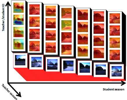
Figure 1: We address the task of sequential multi-domain visual place recognition (SMD-VPR) [4] from the novel perspective of multi-teacher multi-student knowledge distillation (MTMS-KD) [3]. For each $t$-th season ($t$-th column), the teacher set consists of $K$ previous seasons CNNs (1st, 2nd, 3rd and 4th rows), and a tentative CNN that is pretrained on the current season’s training set (5th row). We present a novel recursive knowledge distillation (RKD) framework that recursively compresses all the previous seasons’ knowledge (i.e., 1st, $\cdots$, $(t-1)$-th columns) into a constant size CNN ensemble (i.e., $t$-th column).

We further address a key question in RKD, termed the teacher-student assignment (TSA) problem: “which student should be trained by which teacher?” The TSA problem itself is difficult and it involves a generalization/specialization tradeoff: if a student’s CNN is trained by a specific season’s teacher, its season-specific VPR ability will increase, while its generic VPR ability will decrease. Thus, we have two possible choices: either we train a specific student’s CNN with a specific teacher’s CNN or we do not, and we have exponential number of possible choices to the number of experienced seasons. Searching the best choice in this large number of possible TSAs is often unfeasible. We explore and discuss several strategies for the TSA problem.

The main contributions of our work are as follows:

1. We propose a novel sequential-multi-domain CS-VPR (SMD-VPR) framework, which requires a constant cost for long-term memory and retraining.

2. We frame the SMD-VPR task as a recursive KD (RKD) and address the novel TSA problem.

In this study, we formulate the SMD-VPR as a CNN-based classification problem, and focus on the issue of long-term RKD and TSA. Further, in this study we extend our previously developed long-term ensemble learning (LEL) framework [5, 4] to a memory efficient MTMS-KD system. In [5], we developed a recursive MTMS framework whereby teachers’ CNNs in the previous season are directly retrained into the current season’s CNNs, which can then be used as student CNNs. In [4], we addressed the issue of space efficiency in the MTMS framework for the first time, and presented an efficient MTMS framework by representing a CNN as a collection of season-specific training images. However, such frameworks require to explicitly store a number of training images proportional to the number of experienced seasons and places, which severely limits the scalability to long-term large-size SMD-VPR tasks.

II Approach

The long-term map learning framework consists of two alternately repeated missions (one iteration per season): exploration and adaptation. The system is initialized with a size one classifier set $S^{1}$$=\{c_{1}^{1}\}$, which consists of a single CNN classifier $c^{1}_{1}$ that is obtained by pretraining a CNN using the first season’s training data. A new classifier set $S^{t}=$$\{c_{j}^{t}\}_{j=1}^{K_{t}}$ is then obtained by a teacher-to-student KD in each $t$-th iteration ($t>1$). In experiments, for the initial CNN classifier $c_{1}^{1}$, we use the CNN architecture pretrained on the CIFAR10 dataset, and we consider one iteration of the two missions per season.

The exploration mission aims at maximum possible vehicle exploration of the entire environment, while keeping track of the vehicle’s global position (e.g., using pose tracking [6] and relocation [7]), to collect mapped images that have global viewpoint information, and optionally, the collected data may be further post-processed to refine the viewpoint information by structure-from-motion (SfM) [8] or SLAM [9].

All the collected images that have viewpoint information can be used as training data for the subsequent $t$-th adaptation mission. We denote training data that is collected in the $t$-th exploration as $D^{t}=\{(v,I)\}$, where $I$ and $v$ are an image and its viewpoint, respectively.

Given a set of previous season’s $K^{t-1}$ teacher CNNs and the current season’s train set, the objective of MTMS-KD is to train a new set of current season’s $K^{t}$ student CNNs.

Although our approach is sufficiently general and applicable to generic variable size teacher/student CNN sets, in this study, we focus on simple constant size CNN sets (i.e., $K^{t}=K^{t-1}$) with $K=4$.

To solve this problem, we develop two different types of algorithms: (1) the TSA algorithm which assigns best teachers to each student, and (2) the RKD algorithm which trains a new set of current season’s $K$ student CNNs, from the previous season’s $K$ teacher CNNs and the current season’s training images, given a specific teacher-student-assignment.

II-A Performance Metric

The performance metric of a VPR system is based on the top-$X$ accuracy. In it, the CNN ensemble is modeled as a ranking function, which outputs a ranked list of place classes in descending order of relevance score (e.g., confidence). Then, the accuracy of top-$X$ in the ranked list is evaluated with respect to the ground-truth viewpoint obtained by GPS measurements.

Because the both subtasks are highly ill-posed and no ground-truth solutions (GTs) are available, we investigate the relative performance of metrics that do not rely on ground-truth TSA and RKD, but only require GT viewpoint information. To evaluate the long-term SMD-VPR performance, the above top-$X$ accuracy is evaluated by using the latest up-to-date CNN ensemble. Naturally, the evaluation is performed after rather than before the $t$-th adaptation mission in each $t$-th season.

To evaluate the generalization ability of our VPR system, we use the next season’s unseen data as the test data for the current season’s ensemble. Note that this means that students are often tested with test data of unseen seasons, which the students and previous teachers have never experienced before. This makes our CS-VPR a very challenging problem.

TABLE I: TSA Strategies.

#1	$A_{4}([1,1],1.0)$	#2	$A_{4}([2,2],0.5)$
#3	$A_{4}([2,2],1.0)$	#4	$A_{4}([3,3],1.0)$
#5	$A_{4}([1,2],1.0)$	#6	$A_{4}([0,2],1.0)$
#7	$B_{4}$	#8	$A_{4}([0,4],1.0)$
#9	$B_{2}+A_{2}([0,0],1.0)$	#10	$B_{2}+A_{2}([2,2],1.0)$
#11	$B_{2}+A_{1}([1,1],1.0)+A_{1}([1,1],1.0)$
#12	$B_{2}+A_{2}([1,1],1.0)$	#13	$C_{4,2}$
#14	$A_{4}([0,0],1.0)$

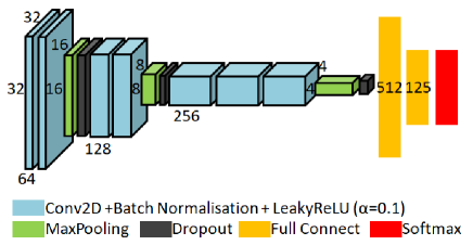
Figure 2: CNN architecture.

II-B TSA

The TSA task aims to achieve a good balance between knowledge transferring from current season’s teacher and previous seasons’ teachers. However, finding a way to achieve such a balance is not straightforward. Instead, we have developed several possible strategies and investigated their effectiveness. In this study, we consider 14 different strategies #1, $\cdots$, #14, as listed in Table I. In these strategies, $A_{s}$ and $B_{s}$ are two different functions that take a size $s$ $(s\in[1,K])$ collection of the previous season’s CNNs $S^{t-1}=$$\{c_{1}^{t-1}$, $\cdots$, $c_{s}^{t-1}\}$, and outputs a $(s+1)\times s$ binary matrix called the TSA matrix $M=\{M_{ij}\}$. An assignment $M_{ij}$ is represented by a connection between a $i$-th teacher CNN and for the $j$-th student CNN. A teacher CNN can be either a previous season’s CNN $c^{t-1}_{i}$$(i>0)$ (denoted as “previous teacher”) or a tentative CNN $c^{t}_{0}$ that is pretrained on the current season’s training set (denoted as “current teacher”). We use an identical CNN architecture for all the CNNs for previous and current season’s teachers. A TSA $M_{ij}$ for $j$-th student CNN represents the assignment of the previous teacher $c^{t-1}_{i}$, where $M_{0j}=1$ represents the assignment of the current teacher $c^{t}_{0}$, and $M_{ij}=1(i>0)$ represents the assignment of the previous $i$-th teacher $c^{t-1}_{a_{i}}$. The main difference between the set functions $A_{s}$ and $B_{s}$ lies in the way the number of teachers are determined. The number of previous season’s teachers is dependent on the number of current season’s teachers for the function $A_{s}$, while it is independent for the functions $B_{s}$. The function $A_{s}([a,b],p)$ samples the number of previous season’s teachers in the range $[a,b]$, and determines whether to use the current season’s teacher with the probability of $p$. The function $B_{s}$ does not distinguish the two teacher types (i.e., previous or current) but simply samples the total number of teachers in range $[1,s]$. The function $C_{s,s^{\prime}}$ $(s^{\prime}<s)$ splits the students into the groups $\{1,\cdots,s^{\prime}\}$, and $\{s^{\prime}+1,\cdots,s\}$, for the former group, it assigns previous and/or current teachers with the number of teachers in range $[1,5]$, while for the latter group, it only assigns the current season’s teacher (i.e., $i=0$). It is worth noting that the method #14 enforces the use of only current season’s teachers. It is viewed as the baseline method in the experimental section III.

II-C Training Procedure

We use an identical CNN architecture for all the teachers and student CNNs. The CNN architecture is based on the one in the CIFAR10 [10]. It consists of 16 layers and the LeakyReLU activation function is employed for each layer. Fig. 2 illustrates the CNN architecture. For the distillation, the training data consists of 25,966 samples from a dataset “2012/5/26” which is independent of training/test data used in experiments. The Adam optimizer [11] is used with a learning rate of 0.003, $\beta_{1}=0.9$, $\beta_{2}=0.999$, $\epsilon=10^{-8}$, and a weight decay of 0. For the loss function, the following soft loss is used.

$$Loss_{softmax}=-\sum_{i}p_{i}\log(q_{i}),$$ (1)

where

$$q_{i}=\frac{exp(z_{i}/T)}{\sum_{j}exp(z_{j}/T)},$$ (2)

$$p_{i}=\frac{exp(v_{i}/T)}{\sum_{j}exp(v_{j}/T)},$$ (3)

where $z_{i}$ and $v_{i}$ are the $i$-th class logits from the student and teacher CNNs, respectively. The temperature $T$ is set to 1 for pretraining and to 10 for KD.

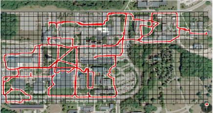
Figure 3: NCLT dataset and definition of place classes. Each place class corresponds to 20$\times$20 $[m^{2}]$ grid cell.

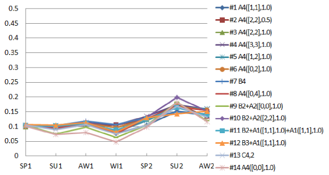
Figure 4: Top-1 accuracy.

III Experiments and Discussions

We evaluated the proposed SMD-VPR framework on a challenging cross-season dataset: a public NCLT dataset [12]. The NCLT is a large-scale, long-term autonomy dataset for robotics research that was collected at the University of Michigan’s North Campus by a Segway vehicle platform. The data we used in this study includes view image sequences along the vehicle trajectories acquired by the front facing camera of the Ladybug3 platform (Fig. 3). Specifically, we used a length 8 sequence of datasets: “2012/3/31 (SP1)”, “2012/8/4 (SU1)”, “2012/11/17 (AU1)”, “2012/1/22 (WI1)”, “2012/5/11 (SP2)”, “2012/8/20 (SU2)”, “2012/11/16 (AU2)”, and “2012/1/8 (WI2)”. For each dataset, we impose a regular 20$\times$20 $[m^{2}]$ grid, and view each cell as a place class candidate. The number of training/testing images are very different between different place cells and is dependent on the viewpoint trajectories followed by the vehicle for each dataset. We ignore the place cells that have an insufficient number of training/testing images for at least one dataset. Consequently, 125 place cells are determined to be valid and are used for our VPR tasks.

Figure 4 shows the performance of each method in each season. The performance in terms of Top-$X$($X$=1, 5, 10) accuracy is investigated for two standard ensemble strategies, namely “averaging” and “merge+sort”. The method #14 is the baseline method as described in Section II-B. One can see that the proposed methods outperformed the baseline method in most of the experiments.

References

- [1] M. J. Milford and G. F. Wyeth, “Seqslam: Visual route-based navigation for sunny summer days and stormy winter nights,” in Robotics and Automation (ICRA), 2012 IEEE International Conference on. IEEE, 2012, pp. 1643–1649.
- [2] A. Krizhevsky, I. Sutskever, and G. E. Hinton, “Imagenet classification with deep convolutional neural networks,” in Advances in neural information processing systems, 2012, pp. 1097–1105.
- [3] Y. Chebotar and A. Waters, “Distilling knowledge from ensembles of neural networks for speech recognition.” in Interspeech, 2016, pp. 3439–3443.
- [4] N. Yang, K. Tanaka, Y. Fang, X. Fei, K. Inagami, and Y. Ishikawa, “Long-term vehicle localization using compressed visual experiences,” in 21st International Conference on Intelligent Transportation Systems, 2018, pp. 2203–2208.
- [5] X. Fei, K. Tanaka, Y. Fang, and A. Takayama, “Long-term ensemble learning for cross-season visual place classification,” JACIII, vol. 22, no. 4, pp. 514–522, 2018.
- [6] S. Wang, R. Clark, H. Wen, and N. Trigoni, “Deepvo: Towards end-to-end visual odometry with deep recurrent convolutional neural networks,” in 2017 IEEE International Conference on Robotics and Automation (ICRA), 2017, pp. 2043–2050.
- [7] E. Garcia-Fidalgo and A. Ortiz, “ibow-lcd: An appearance-based loop-closure detection approach using incremental bags of binary words,” IEEE Robotics and Automation Letters, vol. 3, no. 4, pp. 3051–3057, 2018.
- [8] J. DeGol, T. Bretl, and D. Hoiem, “Improved structure from motion using fiducial marker matching,” in Proceedings of the European Conference on Computer Vision (ECCV), 2018, pp. 273–288.
- [9] J. Engel, T. Schöps, and D. Cremers, “Lsd-slam: Large-scale direct monocular slam,” in European Conference on Computer Vision. Springer, 2014, pp. 834–849.
- [10] A. Krizhevsky and G. Hinton, “Convolutional deep belief networks on cifar-10,” Unpublished manuscript, vol. 40, no. 7, 2010.
- [11] D. P. Kingma and J. Ba, “Adam: A method for stochastic optimization,” arXiv preprint arXiv:1412.6980, 2014.
- [12] N. Carlevaris-Bianco, A. K. Ushani, and R. M. Eustice, “University of michigan north campus long-term vision and lidar dataset,” The International Journal of Robotics Research, pp. 1023–1035, 2015.