Eccentric Binary Black Holes with Spin
via the Direct Integration of the Post-Newtonian Equations of Motion

Abstract

We integrate the third and a half post-Newtonian equations of motion for a fully generic binary black hole system, allowing both for non-circular orbits, and for one or both of the black holes to spin, in any orientation. Using the second post-Newtonian order expression beyond the leading order quadrupole formula, we study the gravitational waveforms produced from such systems. Our results are validated by comparing to Taylor T4 in the aligned-spin circular cases, and the additional effects and modulations introduced by the eccentricity and the spins are analyzed. We use the framework to evaluate the evolution of eccentricity, and trace its contributions to source terms corresponding to the different definitions. Finally, we discuss how this direct integration equations-of-motion code may be relevant to existing and upcoming gravitational wave detectors, showing fully generic, precessing, eccentric gravitational waveforms from a fiducial binary system with the orbital plane and spin precession, and the eccentricity reduction.

I Introduction

The direct detections of gravitational waves (GWs) Abbott et al. (2016a); Abbott et al. (2016b, 2018a) by the LIGO/VIRGO Collaboration Aasi et al. (2015); Acernese et al. (2015); Abbott et al. (2018b) have launched the era of multi-messenger astrophysics, both in providing a new window on events such as binary neutron star (BNS) mergers Abbott et al. (2017a), and by opening for study a completely new field of astrophysical events previously invisible to us, binary black hole (BBH) mergers Abbott et al. (2018a), meriting the Nobel Prize in Physics in 2017.

GWs from eccentric binaries Gopakumar and Iyer (2002); Yunes et al. (2009); Huerta et al. (2014); Hannam et al. (2014); Taracchini et al. (2014); Tanay et al. (2016); Huerta et al. (2017, 2018); Hinder et al. (2018); Lower et al. (2018); Huerta et al. (2019) have become an important topic of study as the next observing runs of the Advanced Laser Interferometer Gravitational-wave Observatory (aLIGO) and VIRGO approach. While it is not expected that LIGO/VIRGO sources in isolated binaries will have significant eccentricity in band, binaries in dense stellar clusters Merritt (2013) may, however, retain significant eccentricity from dynamical interactions prior to entry into the LIGO/VIRGO band. Recent simulations of globular clusters indicate that a distinct population of compact binaries exist (from Refs. Rodriguez et al. (2018, 2016), about 3% of binaries) and enter the LIGO/VIRGO band (canonically taken to be $10$ Hz as the lower bound) with significant eccentricity ($e>0.1$) Rodriguez et al. (2018); Antonini and Rasio (2016). These results add further motivation, for if binaries can form and merge in this way, then there will be a minority (but a distinct minority), that will enter with eccentricity, and which may be missed without templates for the match filtering.

In addition, a large fraction of binaries in globular clusters will have significant eccentricity ($\sim 50\%$ of in-cluster mergers) and will be detectable for the entirety of the LISA band ($\sim 10^{-3}$ – $10^{-1}$ Hz) Breivik et al. (2016); D’Orazio and Samsing (2018). Both 2-body mergers (highly eccentric in cluster mergers in between single binary interactions) and 3-body mergers (when a BBH forms with such high eccentricity that it is essentially a GW capture before it can interact with a third body) will occur in clusters. LISA will be able to measure the 2-body mergers, but not the 3-body mergers Samsing and D’Orazio (2018). Current work is being carried out to see if detection of eccentric sources will be possible with the proposed space-based detector, and current prospects look promising D’Orazio and Samsing (2018); Breivik et al. (2016); Sesana (2016).

In this paper, we develop and calculate the GW waveforms and orbital dynamics from generically spinning, eccentric BBHs. We use the Lagrangian formulation of the post-Newtonian (PN) equations of motion (EOM) in the harmonic gauge for the generation of precessing, eccentric GW signatures Blanchet et al. (1995); Blanchet (1995, 1996); Blanchet et al. (1998); Blanchet (2006); Will (2005); Faye et al. (2006); Blanchet et al. (2006); Will (2011); Marsat et al. (2013); Bohe et al. (2013); Blanchet (2014); Marsat (2015); Bohe et al. (2015); Bernard et al. (2018). Our approach allows us to use any spin values, mass ratios, and eccentricities, without restricting to planar orbits or co-precessing frames, so long as the binary has a large enough separation (around a periapsis passage of $r\sim 10M$), such that the underlying PN theory does not break down Poisson (1995); Mino et al. (1997); Yunes and Berti (2008); Zhang et al. (2011); Sago et al. (2016); Fujita et al. (2018). This approach offers a major step forward as a way to generate eccentric, precessing GW waveforms in a direct and straightforward way, without carrying any of the additional restrictive assumptions of quasi-ellipticity or adiabaticity that many current waveform generators use. Furthermore, we can give more precise waveforms since we do not ignore any timescale effect (see, e.g., Ref. Klein et al. (2018)).

This work is an extension of work first done by Lincoln and Will Lincoln and Will (1990), and of integrations as in Refs. Pati and Will (2000, 2002). In more recent works, Refs. Levin et al. (2011) and Csizmadia et al. (2012) used this framework to 3.5PN to generate eccentric binaries in the PN harmonic gauge, and calculate the relevant waveforms. The research focus of this project is to calculate the orbital quantities and GW waveforms from generic binaries with the requisite accuracy to enable potential future observations from GW detectors. This paper details the methodology, and extends the previous work done by other authors by giving quantitative comparisons to other known PN methods for the first time.

This Lagrangian formulation has larger applications as well. Developing a general EOM that can handle arbitrarily precessing and eccentric BBHs means that we can apply this EOM to the precessing spacetime developed in our previous work Nakano et al. (2016). We must have an accurate EOM for the general precessing BBH that can handle the orbital plane precession of the binary due to spin coupling with the orbit Owen et al. (1998), and also the individual spins precessing in order to evolve the BBH. The Lagrangian formulation excels at all of these, and can directly be used for this evolution.

The regime of final inspiral to plunge and merger can only be modeled by numerical relativity Pretorius (2005); Campanelli et al. (2006a); Baker et al. (2006); Campanelli et al. (2006b); Campanelli et al. (2006); Campanelli et al. (2007a, b); Lousto and Healy (2015); Lousto et al. (2016). This does, however, provide us a unique opportunity to use the numerical relativity regime; we can stitch our PN evolution onto the beginning of NR simulations, and thus create a full waveform model for the binary using hybridization of waveforms Campanelli et al. (2009); Ajith et al. (2012).

This paper is organized as follows. Sec. II gives an overview of the PN EOMs for generic spins and eccentricities. Sec. III shows the power and flexibility of the EOM code, and demonstrates our main results with orbital and waveform quantities for some fiducial systems with eccentricity and spins. Sec. IV quantifies the comparisons of the EOM code with the Taylor T4 method, the initial conditions for quasi-circular orbits, including orbital frequency comparison, and waveform overlaps. In Sec. V, we discuss a simple test of orbital eccentricity by using the EOM. Sec. VI contains discussion, conclusions, and future work.

Throughout this paper, we use the geometric unit system, where $c=G=1$, with the useful conversion factor $1M_{\odot}=1.477\;{\rm{km}}=4.926\times 10^{-6}\;{\rm{s}}$, although we will keep some $1/c$ factors to count PN orders.

II post-Newtonian Formulation

II.1 Orbital Position and Spin Equations of Motion

The general case of unaligned spins (i.e., spins that are neither aligned nor anti-aligned with the orbital angular momentum) leads to precession of the individual spins as well as precession of the orbital angular momentum vector, and therefore precession of the orbital plane. To describe this complicated motion requires two sets of evolution equations: one set describing the positions (trajectories) of the point masses, and one set describing the evolution of the spin of each point mass. We will review the position equations first, then the precession equations. There are several PN papers that go through this in detail. See Ref. Blanchet (2014) for the non-spinning terms, and Refs. Marsat et al. (2013); Bohe et al. (2013) for the spin dependent terms.

The system comprises of two bodies ($a=1,2$), each described by a mass $m_{a}$, a spin $\vec{S}_{a}$, a spin precession vector $\vec{\Omega}_{a}$, and position and velocity vectors $\vec{r}_{a}$, $\vec{v}_{a}$. We also define the total combinations $M=m_{1}+m_{2}$ for the total mass, $\eta=m_{1}m_{2}/M^{2}$ for the symmetric mass ratio, $\mu=M\eta$ for the reduced mass, and

$$\vec{S}=\vec{S}_{1}+\vec{S}_{2}\,,$$ (1)

for the total spin, as well as the relative combinations $\vec{r}=\vec{r}_{1}-\vec{r}_{2}=r\hat{n}$ (where $r=|\vec{r}|$) denoting the relative separation vector, $\vec{v}=\vec{v}_{1}-\vec{v}_{2}$ for the relative velocity, and the relative spin difference $\vec{\Sigma}$, given by

$$\frac{\vec{\Sigma}}{M}=\frac{\vec{S}_{2}}{m_{2}}-\frac{\vec{S}_{1}}{m_{1}}\,.$$ (2)

The schematic EOM for the orbital positions, in terms of relative variables and in the center-of-mass frame, then takes the form:

$$\frac{\mathrm{d}\vec{v}}{\mathrm{d}t} = -\frac{M}{r^{2}}\left[(1+{\mathcal{A}})\hat{n}+{\mathcal{B}}\vec{v}\right]$$ (4)

$$+{\mathcal{C}}_{1}\,(\hat{n}\times\vec{S})+{\mathcal{C}}_{2}\,(\hat{n}\times\vec{\Sigma})$$

$$+{\mathcal{C}}_{3}\,(\vec{S}\times\vec{v})+{\mathcal{C}}_{4}\,(\vec{\Sigma}\times\vec{v})\,,$$

with the non-spinning components of these $\mathcal{A}$ and $\mathcal{B}$ terms defined in Ref. Blanchet (2014), and the spin terms and expressions for ${\mathcal{C}}_{1}$, ${\mathcal{C}}_{2}$, ${\mathcal{C}}_{3}$, and ${\mathcal{C}}_{4}$ defined in Refs. Faye et al. (2006); Blanchet et al. (2006); Marsat et al. (2013); Bohe et al. (2013).

The corresponding precession equations from Ref. Bohe et al. (2013) take the form:

$$\frac{\mathrm{d}\vec{S}}{\mathrm{d}t} = \frac{m_{1}\vec{\Omega}_{1}+m_{2}\vec{\Omega}_{2}}{M}\times\vec{S}+\eta(\vec{\Omega}_{2}-\vec{\Omega}_{1})\times\vec{\Sigma}\,,$$ (5a)

$$\frac{\mathrm{d}\vec{\Sigma}}{\mathrm{d}t} = \frac{m_{2}\vec{\Omega}_{1}+m_{1}\vec{\Omega}_{2}}{M}\times\vec{\Sigma}+(\vec{\Omega}_{2}-\vec{\Omega}_{1})\times\vec{S}\,.$$ (5b)

Following Refs. Will (2005); Blanchet et al. (2006); Blanchet (2014), we use the Tulczyjew spin supplementary condition (SSC) to define a spin vector with conserved Euclidean norm. For this SSC, the higher order spin-orbit terms have been derived in Refs. Faye et al. (2006); Blanchet et al. (2006); Marsat et al. (2013); Bohe et al. (2013); Blanchet (2014). The next-to-leading order spin-spin terms were derived in Ref. Bohe et al. (2015), and the leading order cubic-in-spin terms were derived in Ref. Marsat (2015). To date, leading order quartic- and quintic-in-spin contributions to the EOM have not been derived in PN harmonic coordinates with this SSC. See Appendix B for some details.

Up to 3.5PN  order in this formalism, and for maximal spins ($|\vec{\chi}_{\mathrm{a}}|\simeq 1$ where $\vec{\chi}_{\mathrm{a}}=\vec{S}_{\mathrm{a}}/m_{\mathrm{a}}^{2}$), spin-orbit effects contribute to the EOM at 1.5PN, 2.5PN, and 3.5PN. Spin-spin effects contribute at 2PN and 3PN. Cubic-in-spin effects start from 3.5PN. Quartic- and higher order in-spin effects are beyond 3.5PN.

Equations (5a) and (5b), along with the acceleration equation (4) comprise the EOMs of the two-body system. For a given set of initial conditions, this system of ODE’s is easily solved numerically .

We close this section with some brief comments about radiation reaction. Through 3.5PN order (inclusive), radiation reaction effects arise exclusively in the non-spin part of $\mathcal{B}$. Radiation reaction effects first appear in the non-spin part of $\mathcal{A}$ at 6PN. Spin effects enter radiation reaction at 4PN, and radiation reaction effects enter spin contributions at 4PN. Furthermore, for quasi-circular orbits, the non-spin part of $\mathcal{B}$ contains only radiation reaction effects. In that case, radiation reaction is completely controlled to 3.5PN by turning on/off the non-spin part of $\mathcal{B}$.

II.2 Generation of Gravitational Radiation

To calculate the polarization of GWs, $h_{+}$ and $h_{\times}$, we need to define the principle axes for the GWs. In particular, we define $\hat{N}$ which is the radial direction to the observer, $\hat{p}$, which lies along the line of nodes (for our purposes we can set to be along the $y$ axis), and $\hat{q}$ which is orthogonal to $\hat{N}$ and $\hat{p}$ Will and Wiseman (1996). Note that $\hat{N}\neq\hat{p}\times\hat{q}$.

This allows us to define the inclination $i$, and the phase $\phi$, with respect to the Newtonian angular momentum $\vec{L}=\mu\vec{r}\times\vec{v}$ (see Fig. 1).

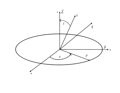
Figure 1: The orbit-adapted vectors for GW polarizations. $\hat{N}$ is the direction to the observer, $\hat{p}$ is along the line of nodes, and $\vec{q}=\hat{N}\times\hat{p}$. The phase of the binary $\phi$ is defined in a right-handed sense. For the initial conditions, the binary starts on the $x$ axis, and the phase is defined from there. The Newtonian angular momentum $\vec{L}=\mu\vec{r}\times\vec{v}$ defines the inclination $i$.

For the GW calculation, we use the 2PN order formula beyond the leading order quadrupole approximation by following Ref. Will and Wiseman (1996):

$$h^{ij} = \frac{2\mu}{R}\bigg{[}Q^{ij}+P^{1/2}Q^{ij}+PQ^{ij}+PQ^{ij}_{\rm SO}$$ (8)

$$\qquad+P^{3/2}Q^{ij}+P^{3/2}Q^{ij}_{\rm SO}+P^{2}Q^{ij}$$

$$\qquad+P^{2}Q^{ij}_{\rm SO}+P^{2}Q^{ij}_{\rm SS}\bigg{]}_{\rm TT}\,,$$

where $R$ denotes the distance between the observer and the binary, and the individual PN terms are broken up into non-spinning, spin-orbit (SO), and spin-spin (SS) contributions. For example, $P^{3/2}Q_{\rm SO}^{ij}$ is the 1.5PN SO contribution, and TT means the transverse-traceless part. We have implemented all of the non-spinning contributions to the quadrupole moment up to 2PN, in order to be in agreement with the GW calculations for Taylor T4.

For the Taylor T4 GW waveforms, we follow Ref. Blanchet (2014), which expands the waveforms $h_{+}$ and $h_{\times}$ into PN orders as powers of the frequency variable $x=(M\Omega)^{2/3}$,

$$h_{+,\times} = \frac{2\mu x}{R}\sum^{+\infty}_{p=0}x^{p/2}H_{(p/2)+,\times}(\psi,\cos i,\sin i;\ln x)$$ (10)

$$+O\bigg{(}\frac{1}{R^{2}}\bigg{)}\,,$$

to the desired PN order. The phase variable $\psi$ is related to the binary orbital phase $\phi$ by the auxiliary phase variable Blanchet (2014):

$$\psi=\phi-2M_{\rm ADM}\Omega\ln\,\bigg{(}\frac{\Omega}{\Omega_{0}}\bigg{)}\,.$$ (11)

The constant frequency $\Omega_{0}$ can be chosen at will, and for our analysis is set to the one related to $10$ Hz (chosen naively as the entry frequency into the LIGO/VIRGO band). The mass variable in the GW calculation is the ADM mass of the binary:

$$M_{\rm ADM}=M\bigg{[}1-\frac{\eta}{2}\gamma+\frac{\eta}{8}(1-\eta)\gamma^{2}+O\bigg{(}\frac{1}{c^{6}}\bigg{)}\bigg{]}\,,$$ (12)

where $\gamma=M/r$ is an expression of the PN parameter of the system. The $H_{(p/2)+,\times}(\psi,\cos i,\sin i;\ln x)$ terms are the specific expansion coefficients, and are dependent on the auxiliary phase variable $\psi$, and the inclination of the binary $i$. The log terms of the frequency variable first occur at 3PN in the GW waveform. Explicit expressions for $H_{(p/2)+,\times}$ appear in Eqs. (322) and (323) of Ref. Blanchet (2014), which can be easily computed from the output of our EOM integrator.

III Eccentric, Precessing Binaries

We now demonstrate the power of our framework for the most generic systems of BBHs, ones with non-unity mass ratios, spin orientations, and eccentricities. Since this parameter space is very large, we use a fiducial example for a demonstration of the orbital and waveform quantities, and know that the formalism is generic for any set of mass, spin, and eccentricity parameters.

For the following example, we follow Ref. Rodriguez et al. (2018) to draw a fiducial binary from the histograms that globular cluster simulations produce. Other than picking physically relevant parameters, we do not restrict ourselves to any particular parameters.

The system that we chose to evaluate is a binary with an initial periapsis passage of $35M$, an initial value eccentricity picked to be $0.4$, a mass ratio $q=3/2$, and dimensionless spin parameter values of $\chi_{1}=(-0.3,0,0)$ and $\chi_{2}=(0,0,0.3)$. The initial periapsis passage and initial eccentricity were selected such that a binary with masses comparable to detected LIGO sources (we use a total mass of 25 solar masses in the analysis of the GW waveform later to dimensionalize the units) would fall just into the LIGO band at periapsis. The chosen spin parameters have low spin to lie in the physically relevant globular cluster results, and are initially strongly misaligned to give lots of spin-spin and spin-orbit precession.

The extrinsic parameters for waveform production that we chose for this fiducial system are optimized for ease. The distance from the source we set to be $500$ Mpc (a redshift of $\sim 0.1$, small enough not to need to take cosmological effects into account), with the orientation set to $(i,\varpi,\Omega)=(0,0,0)$ where $i$, $\varpi$ and $\Omega$ are the extrinsic orbital parameters, and denote the inclination angle, argument of periapsis and longitude of the ascending node, respectively. This is referred to as the optimal orientation, where the binary is face on (inclination equal to zero), the argument of periapsis is set to zero, and the longitude of the ascending node is equal to zero (the binary is not tilted with respect to the observer). These 13 parameters are enough to completely specify the binary that we are describing (though it will not give sky localization, as this set of parameters is only for one detector, and a second detector would be needed for localization purposes). For a real source, it is a straightforward generalization to put in the detector antenna patterns.

The final thing that we will need for the analysis is the eccentricity definition which we use for generic eccentricities. This is given as:

$$e=\frac{r_{\rm max}-r_{\rm min}}{r_{\rm max}+r_{\rm min}}\,,$$ (13)

which is a workable definition of eccentricity for the orbits Levin et al. (2011); Csizmadia et al. (2012) in the situation of non-negligible eccentricity. It is noted that this definition relies on the position of the binary at different points in the orbit; therefore, it is not an instantaneous definition at a point, but is instead averaged over the orbit.

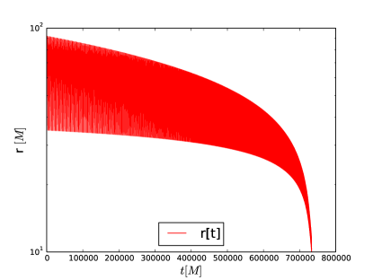
Figure 2: The orbital separation as a function of time for the fiducial system that we lay out below. The binary has an initial periapsis passage of $35M$, an initial eccentricity of $0.4$, a mass ratio $q=3/2$, and initial dimensionless spin parameter values of $\chi_{1}=(-0.3,0,0)$ and $\chi_{2}=(0,0,0.3)$. The orbital eccentricity as the binary evolves is calculated from Eq. (13).

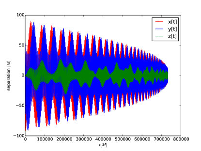
Figure 3: The individual components of the trajectory as a function of time in the center of mass variables for the fiducial binary system that we outlined below. The binary has an initial periapsis passage of $35M$, an initial eccentricity of $0.4$, a mass ratio $q=3/2$, and initial dimensionless spin parameter values of $\chi_{1}=(-0.3,0,0)$ and $\chi_{2}=(0,0,0.3)$. Note here the spin-orbit coupling giving rise to a non zero $z$ component of the orbital motion.

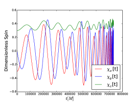
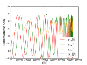
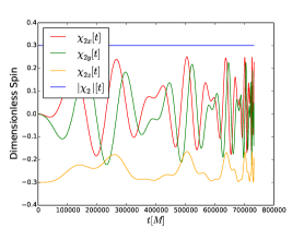
Figure 4: Left: The individual components of the total spin vectors as a function of time for the fiducial binary system that we outlined below. The spins are precessing about the total angular momentum. Center: The individual components of $\vec{\chi}_{1}$ as a function of time. The spin magnitude is conserved in time. Right: The individual components of $\vec{\chi}_{2}$ as a function of time. The spin magnitude is conserved in time. The binary has an initial periapsis passage of $35M$, an initial eccentricity of $0.4$, a mass ratio $q=3/2$, and initial dimensionless spin parameter values of $\chi_{1}=(-0.3,0,0)$ and $\chi_{2}=(0,0,0.3)$.

We start by evolving this binary and plotting the orbital trajectories and spin vectors, shown in Figs. 2, 3, and 4. The eccentricity of the orbit is measured following Eq. (13), from which we calculate the eccentricity in the beginning of the evolution as $e_{\rm init}=0.449$ and the final one as $e_{\rm fin}=0.074$. The discrepancy between the initial eccentricity in the code and the eccentricity that we calculate is due to the setup of the initial conditions, as the initial inputs to the code are calculated as Newtonian initial parameters given a PN $\dot{r}$ and $\omega$, which still does not fully incorporate the PN effects.

The eccentricity reduction can be observed fully in the orbital separation as a function of time (see Fig. 2), and efficiently radiates the eccentricity away over the evolution.

With the orbital quantities, we can calculate the waveforms as well, using the GW waveform prescription in Ref. Will and Wiseman (1996), using the quadrupole formula up to 2PN corrections in Eq. (8). The plus and cross polarizations are tabulated in Figs. 5 and 6.

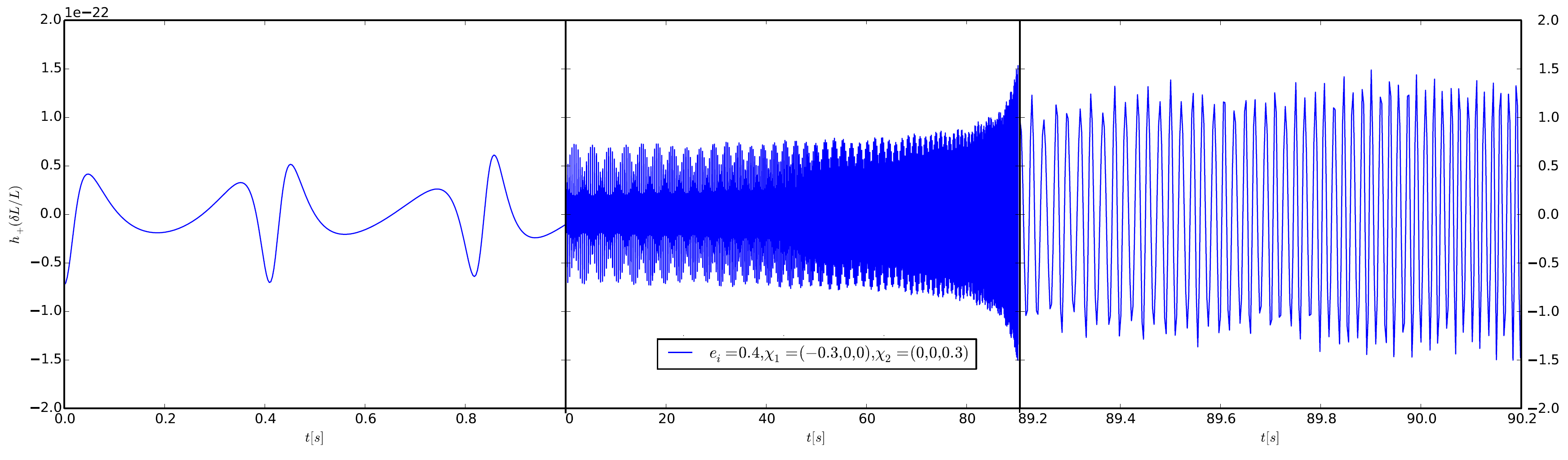
Figure 5: The plus polarization of the GW waveform starting with an eccentricity of $0.4$, and the dimensionless spin vectors $\chi_{1}=(-0.3,0,0)$ and $\chi_{2}=(0,0,0.3)$. The horizontal axis is time in seconds, where we have dimensionalized the units by using a total binary mass of 25 solar masses. The vertical axis is dimensionless strain $\delta L/L$, where we have calculated the strain with a distance to the source at $500$Mpc, and optimal orientation of the binary. See Sec. III for discussion on initial conditions. The measured initial frequencies are $3.5$ Hz at apoapsis, and $10.5$ Hz at periapsis. The measured end frequencies are $55.5$ Hz at apoapsis, and $66.2$ Hz at periapsis. The left and right panels show close-ups of the first and last seconds, respectively. In addition, the spin precession frequency of the GW is roughly $0.1$ Hz.

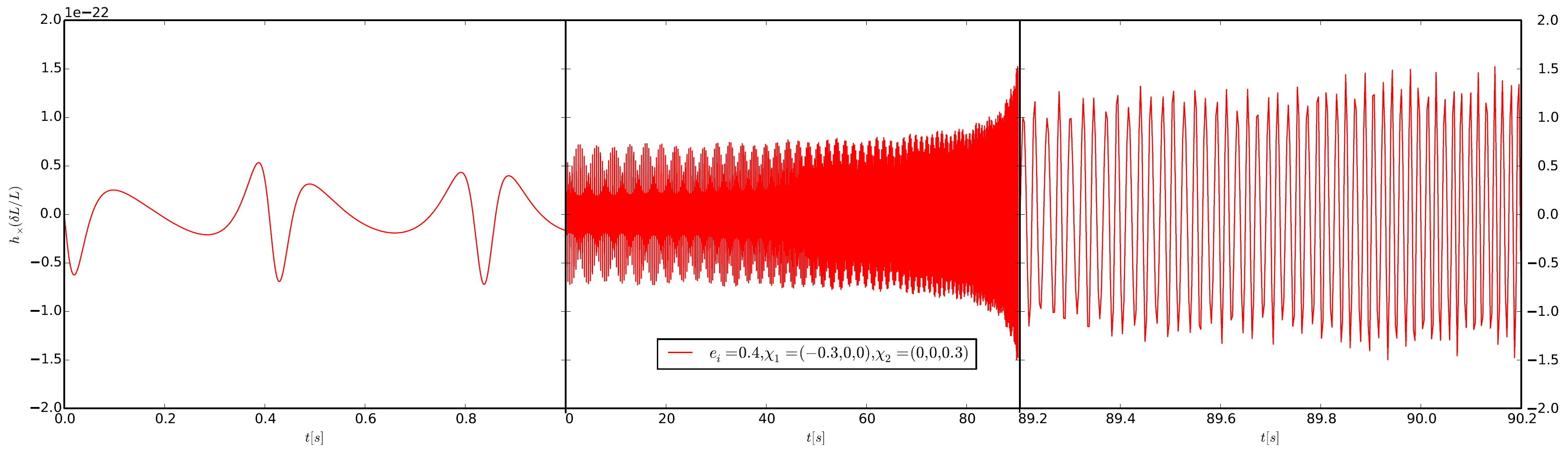
Figure 6: The cross polarization of the GW waveform with the same parameters as the plus polarization shown in Fig. 5. The frequencies are the same as for the plus polarization, but the phase is $90^{\circ}$ off (for this system and orientation).

We calculate the initial and final periapsis and apoapsis GW frequencies directly from the waveform as opposed to an approximate GW frequency from the orbital frequency in order to be as accurate as possible in the calculation of the GW frequency for the entry into a relevant detector (such as LIGO). For this binary, the measured initial frequencies are $3.5$ Hz at apoapsis and $10.5$ Hz at periapsis, and the end frequencies are $55.5$ Hz at apoapsis and $66.2$ Hz at periapsis.

The spin precession frequency is calculated in the same way as the periapsis and apoapsis frequencies by the peak to peak calculation on the waveform. This is not an exact calculation for this frequency, as the spin precession has some ambiguity in the waveform. Since one needs to be able to define the peak in the precessional modulation, this may off by an orbit or two. For the purposes of these calculations, we use the peak amplitude in the waveform for each larger spin precession modulation, getting a value of $0.1$ Hz.

An interesting note with these calculations is that the peak periapsis frequency actually drops with time. This is an artifact of averaging over half an orbit, and when calculating the frequency through $\mathrm{d}\phi/\mathrm{d}t$, this is not an issue. The period in the later stages of the orbit are cleanly broken up into periapsis and apoapsis frequencies. We observe that the sharp periapsis smooths out as the binary circularizes, as expected.

IV Comparisons and Validation

We now turn to comparing the methodology of the direct integration to our implementation of the Taylor T4 method (see Appendix C based on, e.g., Ref. Boyle et al. (2007)), restricted to the case when both should be valid.

Taylor T4 is a PN approximant that assumes quasi-circular, non-precessing orbits. So to compare to Taylor T4, we restrict ourselves to black holes (BHs) that are sufficiently separated, have vanishing orbital eccentricity, and with both spins only along the axis of the orbital angular momentum $\vec{L}$ (each could be either aligned, anti-aligned, or zero).

To begin, we will define a consistent comparison for both Taylor T4 and the direct integration EOMs, and outline the steps needed to reduce to this comparison. We will then compare the orbital frequency and other orbital quantities, and the GW waveforms generated by these systems.

IV.1 Quasi-Circular Orbits in the Direct Integration

Until now we have made no assumptions about eccentricity; all of the expressions to this point are valid for general orbits. Here, we reduce the EOMs to the case of quasi-circular orbits, which is important for our comparisons to other quasi-circular approximants.

To do this, following Ref. Faye et al. (2006), we introduce a moving orthonormal triad $\{\hat{n},\hat{\lambda},\hat{\ell}\}$, where $\hat{n}$ is the same as above, $\hat{\ell}=\hat{n}\times\vec{v}/|\hat{n}\times\vec{v}|$, and $\hat{\lambda}=\hat{\ell}\times\hat{n}$ (see Appendix A). Notice that $\hat{n}$ and $\hat{\lambda}$ span the orbital plane, while $\hat{\ell}$ is normal to it. In this basis, general kinematic considerations lead to the acceleration equation

$$\frac{\mathrm{d}\vec{v}}{\mathrm{d}t}=(\ddot{r}-r\Omega^{2})\hat{n}+(r\dot{\Omega}+2\dot{r}\Omega)\hat{\lambda}+r\varpi\Omega\hat{\ell}\,,$$ (14)

where the dot denotes $\mathrm{d}/\mathrm{d}t$, $\Omega$ is the orbital frequency, and $\varpi$ is the orbital plane precession frequency defined by $\varpi=-\hat{\lambda}\cdot\mathrm{d}\hat{\ell}/\mathrm{d}t$. Quasi-circular orbits $\ddot{r}\simeq\dot{r}\simeq\dot{\Omega}\simeq 0$, the acceleration equation reduces to

$$\frac{\mathrm{d}\vec{v}}{\mathrm{d}t}\simeq-r\Omega^{2}\hat{n}+r\varpi\Omega\hat{\ell}\,.$$ (15)

By identifying Eqs. (15) and (38), one obtains PN expansions for $\Omega^{2}$ and $\varpi$.

Introducing the frequency-related parameter $x\equiv(M\Omega)^{2/3}$ gives a relation $x(\gamma)$, which may then be inverted order-by-order to obtain a relation $\gamma(x)$. With $\gamma(x)$ in hand, one may re-express any function of the coordinate-related parameter $\gamma$ in terms of the frequency-related parameter $x$. This is often preferable, since expressions in terms of the frequency-related parameter are gauge-invariant, whereas expressions in terms of the coordinate-related parameter are not. Examples of quantities that are useful to express as functions of $x$ are the energy, $E(x)$, the flux, $\mathcal{F}(x)$, and the orbital phase, $\phi(x)$. Expressions for these are given in Ref. Ajith et al. (2007) in terms of phase variable $v$ (see Appendix C), and is the jumping off point for the Taylor T4 approximant (see, e.g., Ref. Boyle et al. (2007)).

IV.2 Eccentricity Reduction

For comparing to adiabatic methods such as Taylor T4, we need to be able to accurately and reliably give quasi-circular initial conditions to the direct EOMs numerically. This is more challenging than at first glance, because if we were to simply give Newtonian (or even PN Healy et al. (2017); Ramos-Buades et al. (2019)) initial conditions (detailed above), there would be an error on the order of the neglected PN terms in the initial trajectories. This would manifest as a spurious eccentricity and add undesirable dynamics into the simulation.

We follow a simple procedure to remove this unwanted eccentricity. This procedure has been developed to set up low eccentricity numerical relativity initial data Pfeiffer et al. (2007); Buonanno et al. (2011). We begin by modeling the inspiral as a superposition of two effects, the (real) inspiral, which is a smooth decrease in the orbital separation as a function of time, and the (unphysical) oscillation due to the spurious eccentricity.

We start with a simple assumption for the inspiral part and oscillatory part, namely:

$$\frac{\mathrm{d}r}{\mathrm{d}t}=v_{\mathrm{insp}}(t)+B\cos(\omega\,t+\varphi)\,.$$ (16)

We take the inspiral model $v_{\mathrm{insp}}(t)$ to be a simple polynomial, which we can fit for $v_{\mathrm{insp}}(t)=v_{0}+v_{1}t+v_{2}t^{2}$ with coefficients $v_{0}$, $v_{1}$ and $v_{2}$, and the oscillatory piece $B\cos(\omega\,t+\varphi)$ with the amplitude $B$, frequency $\omega$, and initial phase $\varphi$. With this model, we run our EOM code with the quasi-circular initial conditions detailed above, and fit the data with this model. We can then subtract out the oscillatory piece, and iterate on this model as many times as we need to attain the quasi-circular initial conditions. This is illustrated in Fig. 7.

Mathematically, this is taking the initial conditions $\dot{r}$ and $\Omega$, and after fitting the inspiral, we update

$$\dot{r}_{\rm new}=\dot{r}_{\rm old}+\Delta\dot{r}\,,$$ (17)

and

$$\Omega_{\rm new}=\Omega_{\rm old}+\Delta\Omega\,,$$ (18)

with $\Delta\dot{r}$ and $\Delta\Omega$ given by:

$$\Delta\dot{r} = -B\cos\varphi\,,$$ (19a)

$$\Delta\Omega = -\frac{B\omega\sin\varphi}{2r_{0}\Omega_{0}}\approx-\frac{B\sin\varphi}{2r_{0}}\,,$$ (19b)

where $r_{0}$ is the initial separation of the binary, and $\Omega_{0}$ is the initial orbital frequency.

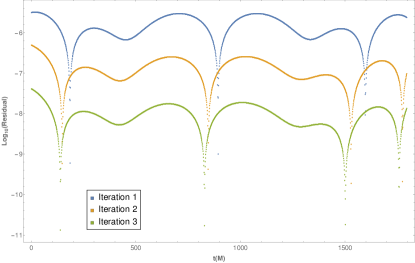
Figure 7: Log of the residuals of $\dot{r}$ in the eccentricity removal from the data and the model (16), over the first three orbits of evolution to refine the initial conditions. This example is at an initial separation of $20M$, with equal masses, and no spin.

IV.3 Consistent PN Order in Taylor T4

The flux formula in Taylor T4 is higher order than what we can calculate in the EOM formalism. To combat this, we need to tailor the T4 fluxes to a consistent PN order. From, e.g., Eq. (A.13) of Ref. Ajith et al. (2007), we can see that the leading order of $v$ is a 2.5PN term. We can also see the series expansion in the flux is out to $v^{7}$, which is 3.5PN beyond leading order. The absolute PN order for the fluxes is then 6PN, which is far beyond the highest order terms in the EOM formalism. To be consistent with our non-adiabatic EOM formalism above, we must truncate the flux terms above next to leading order so that the total re-expanded rational fraction is consistently 3.5PN, i.e., for non-spinning binaries:

$$\mathcal{F}(v) = \frac{32}{5}v^{10}\eta^{2}\bigg{\{}1+v^{2}\bigg{(}-\frac{1247}{336}-\frac{35}{12}\eta\bigg{)}\bigg{\}}\,.$$ (20)

This is what we mean by a “consistent” PN order when we compare to the EOMs in the following sections. When quantifying comparisons, we will use the consistent PN order and the high PN order (keeping the flux terms to 6PN) to track the effects of PN orders.

IV.4 Orbital Frequency Comparison: No Spin

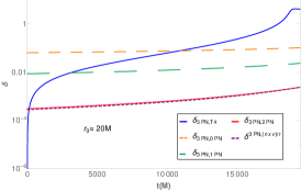
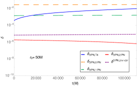
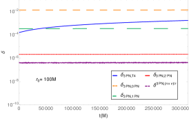
Figure 8: The relative error $\delta({\rm 3PN,Aprx2})$ of the orbital frequencies as a function of time at different PN orders, starting the binary at orbital separations of $r_{0}=20M$ (left), $r_{0}=50M$ (center) and $r_{0}=100M$ (right). All lines compare the 3PN term in Eq. (IV.4) to other approximants. The orange (dashed) line compares 3PN to the Newtonian (0PN) term, so the leading order PN error is 1PN. The green/red (longer-dashed/shortest-dashed) line compare to 1PN/2PN, so the leading order error is 2PN/3PN. The purple (shorter-dashed) line is the relative error of the different orbital frequency definitions for the EOM code, which is similar to the 3PN error for the entire evolution. The blue (solid) line is the relative error between the 3PN EOM code and the consistent PN order Taylor T4.

With the orbital quantities from solving Eq. (51), and the direct EOM orbital quantities from solving Eq. (4), we can explore how to compare these to one another.

First, we need to give both methodologies the same initial conditions, to ensure an apples to apples comparison. This is achieved by using the orbital frequency calculated for the EOM orbit initially (see Eq. (IV.4) below), and setting the initial frequency of the T4 code to the same initial value. This is simple using the relation $\Omega=(v^{3}/M)$, and solving for $\Omega$. We also define the binary phase to start in the same location on the orbit, i.e., the binary starts on the $x$-axis and the angular momentum is defined in the usual right handed sense.

The first and most direct comparisons that we can make are with the orbital frequencies themselves. The orbital frequency via the Taylor T4 method is given by the second integration equation, $\mathrm{d}\phi/\mathrm{d}t=v^{3}/M$, as $\mathrm{d}\phi/\mathrm{d}t=\Omega$.

When we talk about the direct EOM method, however, we need to be careful in how we define the orbital phase. Since EOM method directly outputs the trajectories and velocities, we can calculate the orbital frequency in the Newtonian sense:

$$\Omega=\frac{|\vec{r}\times\vec{v}|}{r^{2}}\,,$$ (21)

which specify the orbital frequency given the orbital trajectories and velocities, $\vec{r}$ and $\vec{v}$. To contrast this, we can use an alternate definition from PN given in Ref. Blanchet (2014) for no spins as

$$\Omega^{2} = \frac{M}{r^{3}}\bigg{\{}1+\bigg{(}-\frac{7}{4}+{1}{4}\eta\bigg{)}\gamma+\bigg{(}-\frac{7}{8}+\frac{49}{8}\eta+\frac{1}{8}\eta^{2}\bigg{)}\gamma^{2}$$

$$+\bigg{(}-\frac{235}{64}+\bigg{[}\frac{46031}{2240}-\frac{123}{64}\pi^{2}+\frac{22}{3}\ln\bigg{(}\frac{r}{r_{0}^{\prime}}\bigg{)}\bigg{]}\eta+\frac{27}{32}\eta^{2}+\frac{5}{64}\eta^{3}\bigg{)}\gamma^{3}\bigg{\}}+O\bigg{(}\frac{1}{c^{8}}\bigg{)}\,,$$

where $r_{0}^{\prime}$ is a gauge constant that we set to $10M$, which is also used in the direct EOM method, and $\gamma$ is the PN parameter $M/r$. This allows us to quantify a PN order by dropping higher order terms and plotting the differences.

For the following analysis, we are restricting to a non-spinning binary in a quasi-circular orbit, that starts in the same initial position for the evolutions of the binary with both Taylor T4 and our direct EOM integration.

We give the results of these different PN orders in Fig. 8 by calculating

$$\delta_{\rm aprx1,aprx2}=\left|\frac{\Omega_{\rm aprx1}-\Omega_{\rm aprx2}}{\Omega_{\rm aprx1}}\right|\,.$$ (23)

We can see immediately that they follow a strict hierarchy of decreasing relative difference as the PN orders are increased, i.e., the differences $\delta_{\rm 3PN,iPN}$ decrease with increasing PN order $i$, which is a good initial sanity check.

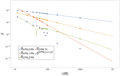
Figure 9: Tracking the PN order of the orbital frequencies as a function of time. We measure the slope of the functional form of the orbital frequency (in solid), through the evolution data (points) for the orbital frequency PN scalings. The T4-EOM comparisons are obtained by fitting the data to a simple polynomial and over plotting the resultant fit function through the data.

We similarly define the difference stemming from using different definitions of the frequency itself,

$$\delta^{\rm def1,def2}=\left|\frac{\Omega^{\rm def1}-\Omega^{\rm def2}}{\Omega^{\rm def1}}\right|\,,$$ (24)

and note that the difference $\delta^{\rm 3PN,n\times v/r}$ accounts for roughly the same order error as the 3PN term (which is reassuring, since the orbital frequency is given to 3PN order in the alternate PN definition stated above). There is a curious thing happening at the initial separation $r=50M$, where this difference $\delta^{\rm 3PN,n\times v/r}$ is larger than the 3PN error. This is explained in Fig. 9, where it becomes apparent that the 3PN term has a zero crossing, and thus dips lower than the difference from the frequency definition. This zero crossing is directly dependent on the gauge term in Eq. (IV.4), and can be shifted at will for different choices of $r_{0}^{\prime}$.

The relative difference of separate PN orders gives a measure of the error in terms of the PN order. We can use this to quantify any comparison in terms of the orbital frequency PN order, and to check the PN scaling of the discrepancies of Taylor T4 and the EOM methods, $\delta_{\rm 3PN,T4}$. What we find is a strong scaling as a function of separation. When the binary is closely separated ($r\leq 12M$), the discrepancy is greater than $1\%$ after an initial discrepancy below the 3PN line. As the binary inspirals, the discrepancy grows, crossing the 2PN line after a short amount of evolution ($t\sim 3000M$), and crosses the 1PN line after ($t\sim 10800M$). When we look at larger separations of $50M$, we see again this same trend of a sharply scaling function of separation, but in this case, it stays below the 2PN line. When we look at the $100M$ case, we find that the discrepancy between the Taylor T4 and EOM codes again stays below the 2PN line, but with a lower relative difference.

Of course, to demonstrate that this is indeed a PN scaling and not another effect, we need to show that the relative differences between the PN orders scale as the proper powers of $r^{s}$ when we look over a large range of separations. We do this in Fig. 9. This figure shows the relative differences scaling as a function of separation. In each case, we fit a power law to the line, and record the slope. The slopes that we find scale with orbital separation $r^{s}$, where the slope $s$ is measured for the individual relative errors. We find that the 1PN error scales with separation as $s\approx-0.976$, the 2PN error scales with separation as $s\approx-1.9995$, the 3PN error scales with separation as $s\approx-4.002$ at far separations ($r\approx 1000M$), and $s\approx-2.7577$ at small separations ($r\sim 12M$). The 3PN error does not scale as $s\approx-3.0$ because of the gauge dependent logarithm term. When looking at separations that are even farther out than $r\approx 100M$, like $r\sim 1000000M$, we find that the slope approaches the correct PN scaling of $-3$. The scaling of the different PN definitions is also tracked here, and while there is not a clear power law trend on this plot, we do note that the definitional discrepancy falls at or below the 3PN line (except for the special case around $50M$), so we can say from this that either definition is acceptable in the EOM code. For our purposes, we will use the geometric definition of $\Omega=|\hat{n}\times\vec{v}|/r$. When we measure the scaling of the Taylor T4–EOM relative error in Fig. 9, we find it is $s\approx-4.545$. We do not attribute this discrepancy to the PN order since this does not obey any obvious PN scaling.

This begs the question of what is causing this rapid drop in relative difference as the separation is increased.

To investigate this, we need to consider what kinds of effects could be at play: this could be a numeric effect (e.g., one of the codes is not calculating to the requisite precision, which is causing a discrepancy at close separations where time steps are smaller); an eccentricity that is deviating the orbit from quasi-circularity in the EOM code; or an effect of the adiabatic approximation breaking down.

To test whether or not this is a numeric effect, we doubled the precision of both codes and re-ran the test at $20M$ again, with the same results. Therefore, we conclude that this is not a numeric issue. To test whether this is an eccentric effect, we ran the EOM code with different levels of the eccentricity remover (which should, in principle, solve the quasi-circularity problem if indeed it is one), and checked the relative differences. We find preliminarily that the residual eccentricity does scale the relative difference of the orbital frequencies, not quite one-to-one, and is removed by the iterative eccentricity removal procedure.

The final plausible possibility is the adiabatic approximation breaking down at close separations, which leads to a high discrepancy between the two methods. This is the most challenging possibility to eliminate. The best method for tracing this is to orbit average all of the EOM code, essentially making it adiabatic. We have done this for the lowest order Peters-Mathews test (0PN (Newtonian) conservative terms, with a 2.5PN radiation reaction term added), and find that this does not seem to affect the evolution at lowest order. Of course, to show that this is indeed unaffected in the general sense, we need to go beyond the leading order evolutions and demonstrate this for 3.5PN.

IV.5 Waveform Comparisons for Aligned Spins and different Mass Ratios

With the orbital frequency analysis concluded, we now turn to calculating the GW waveform overlaps between Taylor T4 and the EOM methods. We pick several fiducial separations, mass ratios, and spins (both aligned and anti-aligned, denoted by $\chi_{1}$ and $\chi_{2}$). The initial separations for which we choose to calculate the overlaps are $100M$, $50M$, and $20M$, with mass ratios $q=m_{2}/m_{1}$ ($m_{2}\geq m_{1}$) of $1$, $2$, $10$, and $100$. The spin parameters that we pick are $\chi_{1}=\{0,0.3,0.6,0.9\}$ and $\chi_{2}=\{0,0.3,0.6,0.9,-0.3,-0.5,-0.6,-0.9\}$, at separations of $50M$ and $100M$.

We calculate the overlap and maximize over time and phase (e.g., Ref. Buonanno et al. (2009)), by calculating the inner product in the frequency domain

$$(h_{1}|h_{2})=4\max_{t_{c}}\bigg{|}\int^{f_{\rm high}}_{f_{\rm low}}\frac{h_{1}^{*}(f,t_{c})h_{2}(f)}{S_{n}(f)}\mathrm{d}f\bigg{|}\,,$$ (25)

where $S_{n}$ is a noise power spectrum density of a detector . The maximization over time is handled by maximizing over $t_{c}$, and the phase maximization is handled by the shifting of $h_{1}$ in the frequency domain. The low frequency cutoff on the integration is set to a reasonable frequency for a detector (for this analysis we set the low frequency cutoff to $10$ Hz, which is a reasonable if a bit ambitious lower frequency bound for LIGO). The high frequency cutoff is not set, to capture the maximum overlap of the waveform if the endpoint is not exactly set to the same frequency.

We then normalize (using the euclidean norm) over $h_{1}$ and $h_{2}$ to obtain the overlap:

$$O=\frac{(h_{1}|h_{2})}{\mathrm{Norm}(h_{1})\mathrm{Norm}(h_{2})}\,.$$ (26)

The results are tabulated in Table 1 (see also Figs. 10 and 11). We keep all of the parameters that we used to calculate the overlaps in the table: the initial and final separations, the mass ratio, the aligned dimensionless spin values $\chi_{1}$ and $\chi_{2}$, the total simulation time in units of $M$, the number of orbits the waveform spanned, the time step of the overlap calculation, and finally the maximized overlap for both the Taylor T4 to EOM comparison at a consistent PN order (3.5PN), and also at the highest T4 order (6PN).

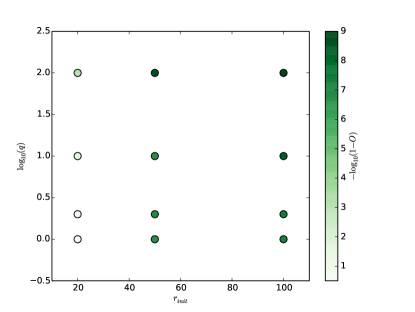
Figure 10: A visualization of the data in Table 1, where we have suppressed all of the spin overlaps, and plot the initial separation vs. the log of the mass ratio, with the color scale indicating $-\log_{10}(1-O)$. This overlap was done over the shortest evolution, at 20M the simulation ran for only 20 orbits, so the rest of the overlaps were calculated for 20 orbits to give an accurate comparison. This parameterization of the color scale leads to the darker colors indicating a better overlap (the number of nines is indicated on the scale).

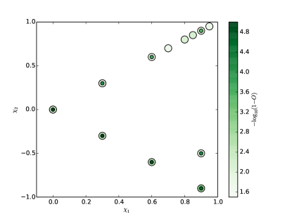
Figure 11: A visualization of the data in Table 1, where we have suppressed the mass ratios and initial separations, and plot the $\chi_{1}$–$\chi_{2}$ plane, with the color scale indicating $-\log_{10}(1-O)$. The large circles indicate an initial separation of $50M$, while some configurations were also examined at $100M$, marked with a smaller inner dot. These overlaps were run on waveforms with a simulation duration of 50 orbits. This parameterization of the color scale leads to the darker colors indicating a better overlap (the number of nines is indicated on the scale).

We see that the overlap is a strong function of the orbital separation: as the separation increases, the overlap increases from a bad overlap at $20M$ of only $O\sim 0.8$ to an overlap of $O\sim 0.99999$ at $100M$. In addition, as the mass ratio increases, the overlap also increases. For example, at a separation of $50M$, holding the spins of the individual BHs to zero, we increase in overlap from $O\sim 0.98$ at $q=1$ to $O\sim 0.99999$ at $q=100$.

When we move to explore the spin parameter space, we hold the mass ratio fixed and compute the overlaps for separations of $100M$ and $50M$. As the dimensionless spin parameter increases in value to higher positive $\chi$ effective ($\chi$ effective is the spin values projected along the orbital angular momentum), the overlap goes down, at $50M$, from $O\sim 0.995$ at spins of zero, to $O\sim 0.99$ at a high positive $\chi$ effective.

When the spins are anti aligned with each other, keeping the effective spin zero, the overlap stays fairly constant, but increases slightly, with the $\chi_{1}=0.9,\,\chi_{2}=-0.9$ having an overlap of $O\sim 0.999$.

A final discussion point is to highlight the effects of PN at higher order with Taylor T4, specifically when we add higher order radiation reaction flux terms. The high order T4 generically differs in overlap from the consistent order T4 by $10^{-8}$ at $100M$, $10^{-5}$ at $50M$, and $10^{-3}$ at $20M$. Though the overlap difference increases as the separation decreases, the PN effects at 4PN do not account for the discrepancy of the overlaps between Taylor T4 and the direct integration EOM.

In addition to the results we tabulate in Table 1, we perform stability tests on the overlap between Taylor T4 and the direct integration EOM by inputting a small $x$-component perturbation to the two spin vectors, which will cause a small amount of spin precession, hence marked ${\rm EOM_{P}}$. Specifically, we give the dimensionless spin vectors $\chi_{1}=(10^{-4},0,0.3)$, and $\chi_{2}=(-10^{-4},0,0.3)$, and we run the same overlaps with the consistent T4 method, and also run the overlap with the EOM code with no $x$-component perturbation to the spins. The overlaps that we obtain are $O_{{\rm T4}-{\rm EOM}}=0.983693663044$, which is exactly the overlap that we obtain when running without the $x$ perturbation. This is easily verifiable by redoing the overlap analysis with the EOM code with and without the perturbation. We obtain an overlap of $O_{{\rm EOM}-{\rm EOM_{P}}}=1.0$, which clearly shows that a perturbation to the spin directions do not affect the overlaps.

V Generic Testbed for Other Approximants: Eccentricity Definitions

This direct EOM that we present is generic and can be applied broadly to many different physical systems, and can be used as a benchmark test for other formalisms. To illustrate this, we apply to a simple test of orbital eccentricity put forward recently Loutrel et al. (2019).

Eccentricity in general relativity is difficult and unintuitive to define Loutrel et al. (2019); Chandrasekhar (1992); Yunes et al. (2009); Memmesheimer et al. (2004). As such, most Newtonian definitions are not sufficient, and can give wildly different results. To illustrate this, we are going to take two different parameterizations of the Newtonian eccentricity, the Runge-Lenz vector and a low eccentricity definition of $e$ used in NR.

The Newtonian Runge-Lenz vector is defined as Poisson and Will (2014):

$$\vec{e}=\bigg{(}\frac{v^{2}}{M}-\frac{1}{r}\bigg{)}\vec{r}-\frac{\vec{r}\cdot\vec{v}}{M}\vec{v}\,,$$ (27)

which, for a Newtonian orbit, is a constant of the motion, and implies that the eccentricity itself is another constant of the motion. To obtain the scalar eccentricity, we simply take the magnitude of this vector. This measure is shown in Fig. 12, in a non-spinning binary system at a low PN order at an initial separation of $20M$, as it evolves down to $10M$.

To contrast this, we will use another definition of eccentricity taken from numerical relativity initial data, using the radial acceleration $\ddot{r}$, following Refs. Campanelli et al. (2009) and Husa et al. (2008). Under the double assumptions of low eccentricity initial data and adiabatic frequency $\Omega$, we can estimate $r(t)$ and its derivatives (to leading order in $e$) by

$$r(t) \sim M^{1/3}\Omega^{-2/3}\left(1+e\sin(\Omega t)\right)~{},$$ (28)

$$\dot{r}(t) \sim M^{1/3}\Omega^{+1/3}e\cos(\Omega t)~{},$$ (29)

$$\ddot{r}(t) \sim -M^{1/3}\Omega^{+4/3}e\sin(\Omega t)~{},$$ (30)

and then define

$$A(t) = \frac{r^{2}\ddot{r}}{M}\sim-e\sin(\Omega t)~{},$$ (31)

so that the eccentricity is given by

$$e=\mathrm{Amp}(A)=\mathrm{Amp}\left(\frac{r^{2}\ddot{r}}{M}\right)\,.$$ (32)

$A(t)$ is also shown in Fig. 12. We note that both measures, as shown in Fig. 12, oscillate – and for $A(t)$, we expect the amplitude of these oscillations to be the actual eccentricity. We thus try to complement $A(t)\sim\sin(\Omega t)$ with the corresponding $\cos(\Omega t)$, using

$$B(t) \doteq \frac{r\dot{r}^{2}}{M}\sim e^{2}\cos^{2}(\Omega t)~{},$$ (33)

and then should have

$$\sqrt{A^{2}+B} = \sqrt{e^{2}\sin^{2}(\Omega t)+e^{2}\cos^{2}(\Omega t)}=e~{}.$$ (34)

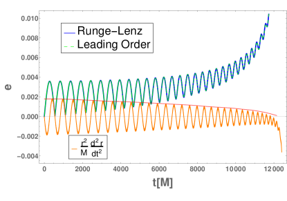
Figure 12: The difference that an eccentricity definition can make in the calculated eccentricity at a given separation. For this figure, the BHs are non-spinning, start at $20M$ separation, and are evolved using the orbital EOM at low order that contains only the 0PN (Newtonian) $+$ 2.5PN (leading-order radiation reaction) terms. The eccentricities are then calculated using the Runge-Lenz definition Eq. (27) (blue), the full NR-derived leading-order measure Eq.  (34) (green), the $\ddot{r}$ formula Eq. (32) (orange), and the amplitude of Eq. (32) (red). The blue and green curves can be seen to be almost identical.

However, in Fig. 12 we see that

1. The curve for $A(t)$ drifts downwards, and at late times oscillates entirely below 0.

2. The curve for $\sqrt{A^{2}+B}$ coincides (to $\sim 1\%$) with the Runge-Lenz eccentricity measure.

3. The curve for $\sqrt{A^{2}+B}$, which is supposed to serve as the non-oscillatory envelope of $A(t)$, does oscillate just like $A(t)$; furthermore, it both starts off above and drifts upwards faster than $A(t)$.

4. The amplitudes of oscillations themselves shrink for both curves (which is what we would have expected the full eccentricity to do).

As all “physical” eccentricities remain very low ($e\sim 10^{-3}$), this suggests that the adiabatic approximation is breaking down; we shall analyze just how:

We no longer take $\Omega$ as a constant, but rather as $\Omega(t)$; we model its leading order behavior as $\Omega(t)\propto\left(t_{c}\!-\!t\right)^{-3/8}$, with $t_{c}$ the projected leading order time of coalescence Abbott et al. (2017b). Then $\dot{\Omega}\sim\Omega/\left(t_{c}\!-\!t\right)$ and $\ddot{\Omega}\sim\Omega/\left(t_{c}\!-\!t\right)^{2}$. We note that for the evolution shown in Fig. 12, $\left(t_{c}\!-\!t\right)$ decreases from $\sim 10^{4}$ to $\sim 10^{3}$, while $\Omega$ changes over a few $\sim 10^{-2}$.

We then see that the derivatives of

$$r(t) \sim M^{1/3}[\Omega(t)]^{-2/3}\left(1+e\sin(\Omega t)\right)$$ (35)

more accurately behave like

$$\dot{r}(t) \sim M^{1/3}\Omega^{+1/3}\left[e\cos(\Omega t)+\alpha\frac{\dot{\Omega}}{\Omega^{2}}+\cdots\right]~{},$$ (36)

$$\ddot{r}(t) \sim -M^{1/3}\Omega^{+4/3}\left[e\sin(\Omega t)+\beta\frac{\ddot{\Omega}}{\Omega^{3}}+\cdots\right]~{},$$ (37)

with numerical factors of order unity, $\alpha$ and $\beta$.

For $\ddot{r}$, when $\left(t_{c}\!-\!t\right)\sim 10^{4}$ the drift term is $\sim\left(t_{c}\!-\!t\right)^{-2}\Omega^{-2}\sim(10^{4})^{-2}(10^{-2})^{-2}=10^{-4}$, and so is smaller than the oscillating eccentricity term $e$; however when $\left(t_{c}\!-\!t\right)\sim 10^{3}$, the drift term grows to $\sim(10^{3})^{-2}(10^{-2})^{-2}=10^{-2}$, and so at late times dominates over the oscillations. This explains why the term $A(t)$ oscillates with the amplitude of the eccentricity early on, but is later dominated by the drift.

For $\dot{r}$ the situation is different: even at early times, $\left(t_{c}\!-\!t\right)\sim 10^{4}$, the drift term, $\sim\left(t_{c}\!-\!t\right)^{-1}\Omega^{-1}\sim(10^{4})^{-1}(10^{-2})^{-1}=10^{-2}$, is already larger than the eccentricity $e$, and so the behavior of $B(t)$ is governed by the drift, rather than the eccentricity oscillations.

As the Runge-Lenz definition Eq. (27) is essentially given by the velocity components, it adopts these features of $\dot{r}$, and measures the drift associated to non-adiabaticity, rather than the eccentricity itself; the eccentricity is given only by the oscillations.

VI Discussion

We have developed and constructed a direct integration of the PN EOM in the harmonic gauge for the construction of eccentric BBHs with arbitrary spins. This work represents a step forward for the modeling of these systems by extending known methods (such as Taylor T4, and the current LIGO/VIRGO collaboration methods) to binaries that evolve the spin procession equations and orbital motion equations for a fully generic GW waveform. This formalism is not limited by eccentricity as the post-Keplerian eccentricity expansion models (e.g., Refs. Gopakumar and Iyer (2002); Yunes et al. (2009); Huerta et al. (2014); Tanay et al. (2016); Hinder et al. (2018)), and is capable of handling eccentricity along with spin precession.

We test the validity of this method by comparing to known results from the Taylor T4 method. In particular, we look at the orbital frequencies produced by systems with the same initial conditions, and compare. The results we find is that the relative difference in the orbital frequencies is a strong function of separation, that does not scale with a high order PN effect, and scales as a function of separation as $r^{s}$ with $s\sim-4.5$.

This effect is not overly worrying, even though we cannot ascribe exactly the cause of this scaling. This is most likely the fundamental difference between Taylor T4 and our method. The various PN dynamics methods do not produce the same results even among the various Taylor T approximants Buonanno et al. (2009). We rule out a numeric issue, and an eccentric effect as the sole cause. We have confirmed that the adiabatic approximation does not affect the evolution of the binary at low order, and are planning on verifying this for the full 3.5PN dynamics in future work.

This begs the question of what is causing this rapid drop in relative difference as the separation is increased.

To investigate this, we need to consider what kinds of effects could be at play: this could be a numeric effect (e.g., one of the codes is not calculating to the requisite precision, which is causing a discrepancy at close separations where time steps are smaller); an eccentricity that is deviating the orbit from quasi-circularity in the EOM code; or an effect of the adiabatic approximation breaking down.

To test whether or not this is a numeric effect, we doubled the precision of both codes and re-ran the test at $20M$ again, with the same results. Therefore, we conclude that this is not a numeric issue. This is an eccentric effect, we ran the EOM code with different levels of the eccentricity remover (which should, in principle, solve the quasi-circularity problem if indeed it is one), and checked the relative differences. We find preliminarily that the residual eccentricity does scale the relative difference of the orbital frequencies, not quite one-to-one, and is removed by the iterative eccentricity removal procedure.

The final plausible possibility is the adiabatic approximation breaking down at close separations, which leads to a high discrepancy between the two methods. This is the most challenging possibility to eliminate. The best method for tracing this is to orbit average all of the EOM code, essentially making it adiabatic. We have done this for the lowest order Peters-Mathews test (0PN conservative terms, with a 2.5PN radiation reaction term added), and find that this does not seem to affect the evolution at lowest order. Of course, to show that this is indeed unaffected in the general sense, we need to go beyond the leading order evolutions and demonstrate this for 3.5PN.

We also compare the GW waveforms of Taylor T4 to the EOM methods, maximizing over time and phase, to give a quantification of the overlap. The results that we find are consistent with the findings of the orbital frequency analysis: the overlap is a strong function of the orbital separation from $20M$ to $100M$. The overlaps increase strongly as a function of mass ratio, with the best overlaps of the waveforms we ran being at a mass ratio $q=100$. In addition, we performed spinning waveform overlaps to test the validity of the spins in the EOM code. We find that the spins do not modify the overlap of the waveform when the effective spin of the binary remains zero, and drops the overlap by about a percent when the spins are aligned and low spins ($\chi_{1}=\chi_{2}=0.3$), to about two percent when the spins are moderately spinning ($\chi_{1}=\chi_{2}=0.6$). The overlap then gets better as the spin gets stronger. We also tested the stability of the code to small perturbations in spin by giving the EOM code a small non-zero spin unaligned with the orbital angular momentum, and found no effect on the overlap.

Finally, we elucidated a fiducial binary system, with realistic parameters drawn from galactic binary simulations, to demonstrate the flexibility and power of this direct integration EOM code. We used initial conditions such that the binary would be in the very low frequency end of the LIGO band at periapsis, and let the binary evolve for 200 orbits. We then output the binary orbital trajectories, spins, and velocities. We recover the orbital plane precession of the binary due to spin-orbit coupling, the spin-spin precession of the individual spins and spin totals, the eccentricity reduction in the binary, and calculate the initial and final eccentricity of the binary using our geometric definition. We take the orbital quantities and calculate the waveform, recovering the eccentric signal imprinted on the outgoing gravitational radiation, estimate the periapsis and apoapsis frequencies of this radiation, and show the spin precession modulation that is also imparted on the binary. We do this for an optimally oriented binary, but leave the code generic so that any binary orientation can be used, providing us with a fully generic, precessing, eccentric binary GW waveform.

We hope to apply this EOM code to parameter estimation for future gravitational wave detections. We currently have the code implemented in Mathematica, and the analysis takes approximately a minute to complete. This is far too long for parameter estimation purposes currently, and we are planning on focusing on this in the future.

There are several relevant detectors for this fiducial source. The periapsis frequency passage is at the threshold of detectability for LIGO/VIRGO at design sensitivity Moore et al. (2015); Martynov et al. (2016); Barsotti et al. (2018); it will fall into the band for future LIGO upgrades such as A+; and third generation ground-based detectors will have both the periapsis and apoapsis frequencies in band.

The precessional frequency will be detectable by planned space based detectors such as the LISA mission Amaro-Seoane et al. (2017), though the source outlined above will be too weak for detection, these frequencies are in band if a nearby binary happens to have these parameters.

We also note that there is a planned Chinese space-borne GW detector in the millihertz frequencies, TianQin Luo et al. (2016), and a planned Japanese space-born detector, DECihertz laser Interferometer Gravitational wave Observatory (DECIGO/B-DECIGO) Seto et al. (2001); Sato et al. (2017) in between the frequency ranges of ground based and LISA detectors. These will make it possible to detect a binary’s dynamics by multiband GW astronomy.

Appendix A Another expression for PN EOM

Equation (4) can be reformulated into the alternate form:

$$\frac{\mathrm{d}\vec{v}}{\mathrm{d}t} =-\displaystyle{\frac{M}{r^{2}}}\bigg{[}(1+\tilde{\mathcal{A}})\hat{n}+\tilde{\mathcal{B}}\vec{v}+\tilde{\mathcal{C}}\hat{\ell}\,\,\bigg{]}\,.$$ (38)

We note that while the unit vector $\hat{\ell}$ is orthogonal to $\hat{n}$ and $\vec{v}$, the triad $\{\hat{n},\vec{v},\hat{\ell}\}$ does not form an orthogonal basis, because $\hat{n}$ and $\vec{v}$ will, in general, not be orthogonal to one another (although they will be approximately orthogonal in the special case of quasi-circular orbits). This equation resembles Eq. (129) in Ref. Blanchet (2014), except for the additional $\tilde{\mathcal{C}}$ coefficient. It is noted that the term with coefficient $\tilde{\mathcal{C}}$ represents a component of the acceleration directed out of the instantaneous orbital plane spanned by $\hat{n}$ and $\vec{v}$. It therefore gives rise to precession of the orbital plane and correspondingly ought to vanish identically when spins are aligned or anti-aligned with the orbital angular momentum.

To obtain Eq. (38), we may expand each cross-product in Eq. (4) by using

$$\hat{n}\times\vec{S} = \dot{r}\tilde{S}_{\ell}\,\hat{n}-\tilde{S}_{\ell}\,\vec{v}+r\Omega\tilde{S}_{\lambda}\,\hat{\ell}\,,$$ (39)

$$\hat{n}\times\vec{\Sigma} = \dot{r}\tilde{\Sigma}_{\ell}\,\hat{n}-\tilde{\Sigma}_{\ell}\,\vec{v}+r\Omega\tilde{\Sigma}_{\lambda}\,\hat{\ell}\,,$$ (40)

$$\vec{S}\times\vec{v} = -v^{2}\tilde{S}_{\ell}\,\hat{n}+\dot{r}\tilde{S}_{\ell}\,\vec{v}+r\Omega(S_{\mathrm{n}}-\dot{r}\tilde{S}_{\lambda})\,\hat{\ell}\,,$$ (41)

$$\vec{\Sigma}\times\vec{v} = -v^{2}\tilde{\Sigma}_{\ell}\,\hat{n}+\dot{r}\tilde{\Sigma}_{\ell}\,\vec{v}+r\Omega(\Sigma_{\mathrm{n}}-\dot{r}\tilde{\Sigma}_{\lambda})\,\hat{\ell}\,,$$ (42)

where $\Omega$ is the instantaneous orbital frequency, $\hat{\lambda}\equiv\hat{\ell}\times\hat{n}$, and we have introduced the notation

$$S_{\ell}=\vec{S}\cdot\hat{\ell}\,,\quad S_{\mathrm{n}}=\vec{S}\cdot\hat{n}\,,\quad S_{\lambda}=\vec{S}\cdot\hat{\lambda}\,,$$

$$\Sigma_{\ell}=\vec{\Sigma}\cdot\hat{\ell}\,,\quad\Sigma_{\mathrm{n}}=\vec{\Sigma}\cdot\hat{n}\,,\quad\Sigma_{\lambda}=\vec{\Sigma}\cdot\hat{\lambda}\,,$$

and

$$\tilde{S}_{\ell}=S_{\ell}/(r\Omega)\,,\quad\tilde{S}_{\lambda}=S_{\lambda}/(r\Omega)\,,$$

$$\tilde{\Sigma}_{\ell}=\Sigma_{\ell}/(r\Omega)\,,\quad\tilde{\Sigma}_{\lambda}=\Sigma_{\lambda}/(r\Omega)\,.$$

The PN expansion for $\Omega$ is only calculated in the case of quasi-circular orbits. To avoid assuming quasi-circular orbits, we may replace $r\Omega$ in the above identities with the (exact) identity

$$r\Omega=|\hat{n}\times\vec{v}|=\sqrt{v^{2}-\dot{r}^{2}}\,.$$ (43)

After using Eqs. (39)–(42) to eliminate the cross-products in Eq. (4) and recollecting terms, one obtains an acceleration equation in the form of Eq. (38), with

$$\tilde{\mathcal{A}} = {\mathcal{A}}-\left(\frac{m}{r^{2}}\right)^{-1}\left[\dot{r}\tilde{S}_{\ell}\,{\mathcal{C}}_{1}+\dot{r}\tilde{\Sigma}_{\ell}\,{\mathcal{C}}_{2}-v^{2}\tilde{S}_{\ell}\,{\mathcal{C}}_{3}-v^{2}\tilde{\Sigma}_{\ell}\,{\mathcal{C}}_{4}\right]\,,$$ (44a)

$$\tilde{\mathcal{B}} = {\mathcal{B}}-\left(\frac{m}{r^{2}}\right)^{-1}\left[-r\Omega\tilde{S}_{\ell}\,{\mathcal{C}}_{1}-r\Omega\tilde{\Sigma}_{\ell}\,{\mathcal{C}}_{2}+\dot{r}\tilde{S}_{\ell}\,{\mathcal{C}}_{3}+\dot{r}\tilde{\Sigma}_{\ell}\,{\mathcal{C}}_{4}\right]\,,$$ (44b)

$$\tilde{\mathcal{C}} = -\left(\frac{m}{r^{2}}\right)^{-1}r\Omega\left[\tilde{S}_{\lambda}\,{\mathcal{C}}_{1}+\tilde{\Sigma}_{\lambda}\,{\mathcal{C}}_{2}+(S_{\mathrm{n}}-\dot{r}\tilde{S}_{\lambda})\,{\mathcal{C}}_{3}+(\Sigma_{\mathrm{n}}-\dot{r}\tilde{\Sigma}_{\lambda})\,{\mathcal{C}}_{4}\right]\,.$$ (44c)

It is noted that this last equation is used in the case of quasi-circular orbits to compute the orbital plane precession frequency $\varpi$. Also we note that in the case when spins are aligned or anti-aligned, $\mathcal{C}$ vanishes identically (since in that case $S_{\mathrm{n}}=\tilde{S}_{\lambda}=0$ and $\Sigma_{\mathrm{n}}=\tilde{\Sigma}_{\lambda}=0$).

Appendix B Spin Precession Equations

We overview the spin precession equations for two bodies with spins that are unaligned with the orbital angular momentum. As mentioned previously, these equations are needed to complete the EOM.

There is no unique definition of center of mass in a relativistic theory. The notion of spin inherits this ambiguity, which gives rise to non-physical degrees of freedom that need to be controlled. This is done by imposing a “spin supplementary condition” (or SSC) that eliminates the non-physical degrees of freedom. The SSC is imposed on the spin tensor, out of which are constructed a spin 4-vector and eventually a spin 3-vector, with just three physical degrees of freedom. Following Refs. Faye et al. (2006); Blanchet et al. (2006); Marsat et al. (2013); Bohe et al. (2013), we use the Tulczyjew SSC Kidder (1995).

$$S^{\mu\nu}p_{\nu}=0\,.$$ (45)

We define spin 3-vectors with conserved norm by $\vec{S}_{\mathrm{a}}$, where $\mathrm{a}=1,\,2$ is the label of the particles. In terms of these conserved norm spin vectors, the precession equations are written as

$$\frac{\mathrm{d}\vec{S}_{\mathrm{a}}}{\mathrm{d}t}=\vec{\Omega}_{\mathrm{a}}\times\vec{S}_{\mathrm{a}}\,,$$ (46)

where $\vec{\Omega}_{\mathrm{a}}$ with $\mathrm{a}=1,\,2$ are the precession vectors for mass 1 and 2, respectively. Each precession vector can be decomposed as

$$\vec{\Omega}_{\mathrm{a}}=\vec{\Omega}_{\mathrm{a,NS}}+\vec{\Omega}_{\mathrm{a,SO}}+\vec{\Omega}_{\mathrm{a,SS}}+O{(SSS)}\,.$$ (47)

The precession vectors are only expanded to quadratic-in-spin order, $O{(SS)}$, because they get multiplied by a spin vector in the precession equation. Terms in the precession vectors at $O{(SSS)}$ would contribute at $O{(SSSS)}$ in the precession equations, which is beyond the scope of this work. Each contribution to the precession vector is then decomposed into a PN expansion of the form,

$$\vec{\Omega}_{\mathrm{a,NS}} = \frac{1}{c^{2}}\vec{\Omega}_{\mathrm{a,NS}}^{(\mathrm{1PN})}+\frac{1}{c^{4}}\vec{\Omega}_{\mathrm{a,NS}}^{(\mathrm{2PN})}+\frac{1}{c^{6}}\vec{\Omega}_{\mathrm{a,NS}}^{(\mathrm{3PN})}$$ (48b)

$$+\frac{1}{c^{7}}\vec{\Omega}_{\mathrm{a,NS}}^{(\mathrm{3.5PN})}+O\left(\frac{1}{c^{8}}\right)\,,$$

$$\vec{\Omega}_{\mathrm{a,SO}} = \frac{1}{c^{3}}\vec{\Omega}_{\mathrm{a,SO}}^{(\mathrm{1.5PN})}+\frac{1}{c^{5}}\vec{\Omega}_{\mathrm{a,SO}}^{(\mathrm{2.5PN})}+\frac{1}{c^{7}}\vec{\Omega}_{\mathrm{a,SO}}^{(\mathrm{3.5PN})}$$ (48d)

$$+O\left(\frac{1}{c^{8}}\right)\,,$$

$$\vec{\Omega}_{\mathrm{a,SS}} = \frac{1}{c^{6}}\vec{\Omega}_{\mathrm{a,SS}}^{(\mathrm{3PN})}+O\left(\frac{1}{c^{8}}\right)\,.$$ (48e)

Explicit expressions for $\vec{\Omega}_{1}$ and $\vec{\Omega}_{2}$ are given in Ref. Bohe et al. (2013).

Appendix C The Taylor T4 Method

Taylor T4 is an adiabatic approximation  that evolves the phase and frequency of the BBH. There are two parts to this method. The first is the phase evolution of the binary, which we will detail here, and the second is the calculation of the gravitational radiation from the orbital phasing of the binary.

All of the formulas of energy and flux can be written in terms of the frequency variable $v\equiv(M\mathrm{d}\phi/\mathrm{d}t)^{1/3}$, and we start with the basic definition of energy conservation, namely:

$$\frac{\mathrm{d}E(v)}{\mathrm{d}t}+\mathcal{F}(v)+\dot{M}(v)=0\,,$$ (49)

where the time rate of change of the energy is equal to the flux leaving the system plus the mass rate of change due to GW absorption. In practice, since this BH absorption is a relatively tiny contribution Isoyama and Nakano (2018) (although 2.5PN order relative to the leading flux), we neglect it for the rest of this analysis, bringing our conservation statement to

$$\frac{\mathrm{d}E(v)}{\mathrm{d}t}=-\mathcal{F}(v)\,.$$ (50)

We start with the energy balance equation (50), integrate it to find $v(t)$, and therefore $\Omega(t)$, since $\mathrm{d}\phi/\mathrm{d}t=\Omega$. Taylor T4 explicitly takes the rational fraction,

$$\frac{\mathrm{d}v}{\mathrm{d}t}=-\frac{\mathcal{F}}{\mathrm{d}E/\mathrm{d}v}\,,$$ (51)

along with

$$\frac{\mathrm{d}\phi}{\mathrm{d}t}=\frac{v^{3}}{M}\,,$$ (52)

re-expands the fraction as a consistent PN series, then numerically integrates to obtain $v(t)$ and $\phi(t)$.

Full expressions of $E(v)$, ${\cal F}(v)$, and $\mathrm{d}E/\mathrm{d}v$ that we use are given in Ref. Ajith et al. (2007). These equations assume a quasi-circular orbit for the trajectory. Taylor T4 approximants integrate the energy balance equations and have been thoroughly explored and developed. Further approximations can be constructed in the frequency domain (the Taylor F-approximants). These methods have been compared, see Ref. Buonanno et al. (2009).

Appendix D Tabulated results on overlap calculations

Separation					Duration			Overlaps $O_{{\rm T4}-{\rm EOM}}$
$r_{\rm init}$ $[M]$	$r_{\rm fin}$ $[M]$	$q$	$\chi_{1}$	$\chi_{2}$	$t$ [M]	orbits	$\mathrm{d}t$ [s]	${\rm T4_{consistent}}$	${\rm T4_{high}}$
100	99	1	0	0	318429.8	$\sim 50$	$1.09061\times 10^{-3}$	0.99999065	0.999990644
100	99	1	0.3	0.3	318429.8	$\sim 50$	$1.04527\times 10^{-3}$	0.99993352	0.999933512
100	99	1	0.6	0.6	318429.8	$\sim 50$	$1.04527\times 10^{-3}$	0.99983625	0.999836244
100	99	1	0.9	0.9	318429.8	$\sim 50$	$1.04527\times 10^{-3}$	0.99971069	0.999710688
100	99	1	0.3	-0.3	318429.8	$\sim 50$	$1.04527\times 10^{-3}$	0.99998949	0.999989489
100	99	1	0.6	-0.6	318429.8	$\sim 50$	$1.04527\times 10^{-3}$	0.9999856287	0.9999856265
100	99	1	0.9	-0.9	318429.8	$\sim 50$	$1.04527\times 10^{-3}$	0.99997797	0.9999778678
100	99	1	0.9	-0.5	318429.8	$\sim 50$	$1.04527\times 10^{-3}$	0.9999415165	0.9999415133
100	99.1	2	0	0	318480.2	$\sim 50$	$1.045439\times 10^{-3}$	0.99999283	0.999992828
100	99.7	10	0	0	318701.62	$\sim 50$	$1.04617\times 10^{-3}$	0.9999991669	0.9999991668
100	99.95	100	0	0	318833.8	$\sim 50$	$1.0466\times 10^{-3}$	0.9999999893	0.9999999893
50	47.2	1	0	0	114043.4	$\sim 50$	$3.90593\times 10^{-4}$	0.994904572	0.994898471
50	47.2	1	0	0	114049.1	$\sim 50$	$2.246257\times 10^{-4}$	0.994797482	0.994791317
50	47.3	1	0.3	0.3	114043.4	$\sim 50$	$3.74357\times 10^{-4}$	0.983693663	0.983675238
50	47.3	1	0.6	0.6	114043.4	$\sim 50$	$3.74357\times 10^{-4}$	0.969583498	0.969553474
50	47.4	1	0.7	0.7	114043.4	$\sim 50$	$3.74357\times 10^{-4}$	0.981885223	0.981867878
50	47.4	1	0.8	0.8	114043.4	$\sim 50$	$3.74357\times 10^{-4}$	0.991724021	0.991717488
50	47.4	1	0.85	0.85	114043.4	$\sim 50$	$3.74357\times 10^{-4}$	0.992601112	0.992597499
50	47.4	1	0.9	0.9	114043.4	$\sim 50$	$3.74357\times 10^{-4}$	0.990197785	0.990190154
50	47.4	1	0.95	0.95	114043.4	$\sim 50$	$3.74357\times 10^{-4}$	0.984804119	0.984791162
50	47.2	1	0.3	-0.3	114043.4	$\sim 50$	$3.74357\times 10^{-4}$	0.995280388	0.995274373
50	47.2	1	0.6	-0.6	114043.4	$\sim 50$	$3.74357\times 10^{-4}$	0.9971254502	0.997121275
50	47.2	1	0.9	-0.9	114043.4	$\sim 50$	$3.74357\times 10^{-4}$	0.9988241423	0.998822279
50	47.3	1	0.9	-0.5	114043.4	$\sim 50$	$3.74357\times 10^{-4}$	0.985182006	0.985164755
50	47.5	2	0	0	114095.5	$\sim 50$	$3.74528\times 10^{-4}$	0.99467073	0.994667208
50	49.1	10	0	0	114299.9	$\sim 50$	$3.75199\times 10^{-4}$	0.999489566	0.999489472
50	49.9	100	0	0	114395.1	$\sim 50$	$3.75512\times 10^{-4}$	0.999994205	0.999994204
20	16	1	0	0	11965	$\sim 20$	$3.92762\times 10^{-5}$	0.782932526	0.775227367
20	18.2	1	0	0	5982.5	$\sim 10$	$1.963812\times 10^{-5}$	0.917453743	0.916892613
20	16.5	2	0	0	11979.2	$\sim 20$	$3.93229\times 10^{-5}$	0.827044247	0.821830277
20	18.8	10	0	0	12050.8	$\sim 20$	$3.95579\times 10^{-5}$	0.972718171	0.97255266
20	19.9	100	0	0	12087.1	$\sim 20$	$3.96769\times 10^{-5}$	0.99919055	0.999190336

Table 1: The overlaps between Taylor T4 and EOM methods, documented for different separations, mass ratios ($q$), and aligned dimensionless spin values ($\chi_{1}$ and $\chi_{2}$), at both the consistent T4 flux order and the highest T4 fluxes available. There are several interesting lines to pay attention to: as the spins increase in alignment, there is an inflection point around $\chi_{1}=\chi_{2}=0.9$, where the overlap drops then increases again. In addition, at $50M$ separation, we increase the resolution of the timestep to probe the effects of numerical resolution on the overlap calculations. We find no effect on the overlap of the waveforms due to the timestep resolution.

References

- Abbott et al. (2016a) B. P. Abbott et al. (Virgo, LIGO Scientific Collaboration), Phys. Rev. Lett. 116, 061102 (2016a), eprint 1602.03837.
- Abbott et al. (2016b) B. P. Abbott et al. (LIGO Scientific, Virgo), Phys. Rev. X6, 041015 (2016b), [erratum: Phys. Rev. X8, 039903 (2018)], eprint 1606.04856.
- Abbott et al. (2018a) B. P. Abbott et al. (LIGO Scientific, Virgo) (2018a), eprint 1811.12907.
- Aasi et al. (2015) J. Aasi et al. (LIGO Scientific), Class. Quant. Grav. 32, 074001 (2015), eprint 1411.4547.
- Acernese et al. (2015) F. Acernese et al. (VIRGO), Class. Quant. Grav. 32, 024001 (2015), eprint 1408.3978.
- Abbott et al. (2018b) B. P. Abbott et al. (VIRGO, KAGRA, LIGO Scientific Collaboration), Living Rev. Rel. 21, 3 (2018b), [Living Rev. Rel. 19, 1 (2016)], eprint 1304.0670.
- Abbott et al. (2017a) B. Abbott et al. (Virgo, LIGO Scientific Collaboration), Phys. Rev. Lett. 119, 161101 (2017a), eprint 1710.05832.
- Gopakumar and Iyer (2002) A. Gopakumar and B. R. Iyer, Phys. Rev. D65, 084011 (2002), eprint gr-qc/0110100.
- Yunes et al. (2009) N. Yunes, K. G. Arun, E. Berti, and C. M. Will, Phys. Rev. D80, 084001 (2009), [Erratum: Phys. Rev. D89, 109901 (2014)], eprint 0906.0313.
- Huerta et al. (2014) E. A. Huerta, P. Kumar, S. T. McWilliams, R. O’Shaughnessy, and N. Yunes, Phys. Rev. D90, 084016 (2014), eprint 1408.3406.
- Hannam et al. (2014) M. Hannam, P. Schmidt, A. Bohé, L. Haegel, S. Husa, F. Ohme, G. Pratten, and M. Pürrer, Physical Review Letters 113, 151101 (2014), eprint 1308.3271.
- Taracchini et al. (2014) A. Taracchini, A. Buonanno, Y. Pan, T. Hinderer, M. Boyle, D. A. Hemberger, L. E. Kidder, G. Lovelace, A. H. Mroué, H. P. Pfeiffer, et al., Phys. Rev. D89, 061502 (2014), eprint 1311.2544.
- Tanay et al. (2016) S. Tanay, M. Haney, and A. Gopakumar, Phys. Rev. D93, 064031 (2016), eprint 1602.03081.
- Huerta et al. (2017) E. A. Huerta et al., Phys. Rev. D95, 024038 (2017), eprint 1609.05933.
- Huerta et al. (2018) E. A. Huerta et al., Phys. Rev. D97, 024031 (2018), eprint 1711.06276.
- Hinder et al. (2018) I. Hinder, L. E. Kidder, and H. P. Pfeiffer, Phys. Rev. D98, 044015 (2018), eprint 1709.02007.
- Lower et al. (2018) M. E. Lower, E. Thrane, P. D. Lasky, and R. Smith, Phys. Rev. D98, 083028 (2018), eprint 1806.05350.
- Huerta et al. (2019) E. A. Huerta et al. (2019), eprint 1901.07038.
- Merritt (2013) D. Merritt, Dynamics and Evolution of Galactic Nuclei (Princeton University Press, Princeton, 2013).
- Rodriguez et al. (2018) C. L. Rodriguez, P. Amaro-Seoane, S. Chatterjee, and F. A. Rasio, Phys. Rev. Lett. 120, 151101 (2018), eprint 1712.04937.
- Rodriguez et al. (2016) C. L. Rodriguez, S. Chatterjee, and F. A. Rasio, Phys. Rev. D 93, 084029 (2016), eprint 1602.02444.
- Antonini and Rasio (2016) F. Antonini and F. A. Rasio, Astrophys. J. 831, 187 (2016), eprint 1606.04889.
- Breivik et al. (2016) K. Breivik, C. L. Rodriguez, S. L. Larson, V. Kalogera, and F. A. Rasio, Astrophys. J. 830, L18 (2016), eprint 1606.09558.
- D’Orazio and Samsing (2018) D. J. D’Orazio and J. Samsing, Mon. Not. Roy. Astron. Soc. 481, 4775 (2018), eprint 1805.06194.
- Samsing and D’Orazio (2018) J. Samsing and D. J. D’Orazio, Mon. Not. Roy. Astron. Soc. 481, 5445 (2018), eprint 1804.06519.
- Sesana (2016) A. Sesana, Phys. Rev. Lett. 116, 231102 (2016), eprint 1602.06951.
- Blanchet et al. (1995) L. Blanchet, T. Damour, and B. R. Iyer, Phys. Rev. D51, 5360 (1995), eprint gr-qc/9501029.
- Blanchet (1995) L. Blanchet, Phys. Rev. D51, 2559 (1995), eprint gr-qc/9501030.
- Blanchet (1996) L. Blanchet, Phys. Rev. D54, 1417 (1996), eprint gr-qc/9603048.
- Blanchet et al. (1998) L. Blanchet, G. Faye, and B. Ponsot, Phys. Rev. D58, 124002 (1998), eprint gr-qc/9804079.
- Blanchet (2006) L. Blanchet, Living Rev. Rel. 9, 4 (2006), eprint gr-qc/0202016.
- Will (2005) C. M. Will, Phys. Rev. D71, 084027 (2005), eprint gr-qc/0502039.
- Faye et al. (2006) G. Faye, L. Blanchet, and A. Buonanno, Phys. Rev. D74, 104033 (2006), eprint gr-qc/0605139.
- Blanchet et al. (2006) L. Blanchet, A. Buonanno, and G. Faye, Phys. Rev. D74, 104034 (2006), eprint gr-qc/0605140.
- Will (2011) C. M. Will, Proceedings of the National Academy of Science 108, 5938 (2011), eprint 1102.5192.
- Marsat et al. (2013) S. Marsat, A. Bohe, G. Faye, and L. Blanchet, Class. Quant. Grav. 30, 055007 (2013), eprint 1210.4143.
- Bohe et al. (2013) A. Bohe, S. Marsat, G. Faye, and L. Blanchet, Class. Quant. Grav. 30, 075017 (2013), eprint 1212.5520.
- Blanchet (2014) L. Blanchet, Living Rev. Rel. 17, 2 (2014), eprint 1310.1528.
- Marsat (2015) S. Marsat, Class. Quant. Grav. 32, 085008 (2015), eprint 1411.4118.
- Bohe et al. (2015) A. Bohe, G. Faye, S. Marsat, and E. K. Porter, Class. Quant. Grav. 32, 195010 (2015), eprint 1501.01529.
- Bernard et al. (2018) L. Bernard, L. Blanchet, G. Faye, and T. Marchand, Phys. Rev. D97, 044037 (2018), eprint 1711.00283.
- Poisson (1995) E. Poisson, Phys. Rev. D52, 5719 (1995), [Addendum: Phys. Rev. D55, 7980 (1997)], eprint gr-qc/9505030.
- Mino et al. (1997) Y. Mino, M. Sasaki, M. Shibata, H. Tagoshi, and T. Tanaka, Prog. Theor. Phys. Suppl. 128, 1 (1997), eprint gr-qc/9712057.
- Yunes and Berti (2008) N. Yunes and E. Berti, Phys. Rev. D77, 124006 (2008), [Erratum: Phys. Rev. D83, 109901 (2011)], eprint 0803.1853.
- Zhang et al. (2011) Z. Zhang, N. Yunes, and E. Berti, Phys. Rev. D84, 024029 (2011), eprint 1103.6041.
- Sago et al. (2016) N. Sago, R. Fujita, and H. Nakano, Phys. Rev. D93, 104023 (2016), eprint 1601.02174.
- Fujita et al. (2018) R. Fujita, N. Sago, and H. Nakano, Class. Quant. Grav. 35, 027001 (2018), eprint 1707.09309.
- Klein et al. (2018) A. Klein, Y. Boetzel, A. Gopakumar, P. Jetzer, and L. de Vittori, Phys. Rev. D98, 104043 (2018), eprint 1801.08542.
- Lincoln and Will (1990) C. W. Lincoln and C. M. Will, Phys. Rev. D42, 1123 (1990).
- Pati and Will (2000) M. E. Pati and C. M. Will, Phys. Rev. D62, 124015 (2000), eprint gr-qc/0007087.
- Pati and Will (2002) M. E. Pati and C. M. Will, Phys. Rev. D65, 104008 (2002), eprint gr-qc/0201001.
- Levin et al. (2011) J. Levin, S. T. McWilliams, and H. Contreras, Class. Quant. Grav. 28, 175001 (2011), eprint 1009.2533.
- Csizmadia et al. (2012) P. Csizmadia, G. Debreczeni, I. Racz, and M. Vasuth, Class. Quant. Grav. 29, 245002 (2012), eprint 1207.0001.
- Nakano et al. (2016) H. Nakano, B. Ireland, M. Campanelli, and E. J. West, Class. Quant. Grav. 33, 247001 (2016), eprint 1608.01033.
- Owen et al. (1998) B. J. Owen, H. Tagoshi, and A. Ohashi, Phys. Rev. D57, 6168 (1998), eprint gr-qc/9710134.
- Pretorius (2005) F. Pretorius, Phys. Rev. Lett. 95, 121101 (2005), eprint gr-qc/0507014.
- Campanelli et al. (2006a) M. Campanelli, C. O. Lousto, P. Marronetti, and Y. Zlochower, Phys. Rev. Lett. 96, 111101 (2006a), eprint gr-qc/0511048.
- Baker et al. (2006) J. G. Baker, J. Centrella, D.-I. Choi, M. Koppitz, and J. van Meter, Phys. Rev. Lett. 96, 111102 (2006), eprint gr-qc/0511103.
- Campanelli et al. (2006b) M. Campanelli, C. O. Lousto, and Y. Zlochower, Phys. Rev. D74, 041501 (2006b), eprint gr-qc/0604012.
- Campanelli et al. (2006) M. Campanelli, C. O. Lousto, and Y. Zlochower, Phys. Rev. D74, 084023 (2006), eprint astro-ph/0608275.
- Campanelli et al. (2007a) M. Campanelli, C. O. Lousto, Y. Zlochower, and D. Merritt, Phys. Rev. Lett. 98, 231102 (2007a), eprint gr-qc/0702133.
- Campanelli et al. (2007b) M. Campanelli, C. O. Lousto, Y. Zlochower, and D. Merritt, Astrophys. J. 659, L5 (2007b), eprint gr-qc/0701164.
- Lousto and Healy (2015) C. O. Lousto and J. Healy, Phys. Rev. Lett. 114, 141101 (2015), eprint 1410.3830.
- Lousto et al. (2016) C. O. Lousto, J. Healy, and H. Nakano, Phys. Rev. D93, 044031 (2016), eprint 1506.04768.
- Campanelli et al. (2009) M. Campanelli, C. O. Lousto, H. Nakano, and Y. Zlochower, Phys. Rev. D79, 084010 (2009), eprint 0808.0713.
- Ajith et al. (2012) P. Ajith, M. Boyle, D. A. Brown, B. Brugmann, L. T. Buchman, et al., Class. Quant. Grav. 29, 124001 (2012), eprint 1201.5319.
- Will and Wiseman (1996) C. M. Will and A. G. Wiseman, Phys. Rev. D54, 4813 (1996), eprint gr-qc/9608012.
- Boyle et al. (2007) M. Boyle, D. A. Brown, L. E. Kidder, A. H. Mroue, H. P. Pfeiffer, M. A. Scheel, G. B. Cook, and S. A. Teukolsky, Phys. Rev. D76, 124038 (2007), eprint 0710.0158.
- Ajith et al. (2007) P. Ajith, M. Boyle, D. A. Brown, S. Fairhurst, M. Hannam, I. Hinder, S. Husa, B. Krishnan, R. A. Mercer, F. Ohme, et al. (2007), eprint 0709.0093.
- Healy et al. (2017) J. Healy, C. O. Lousto, H. Nakano, and Y. Zlochower, Class. Quant. Grav. 34, 145011 (2017), eprint 1702.00872.
- Ramos-Buades et al. (2019) A. Ramos-Buades, S. Husa, and G. Pratten, Phys. Rev. D99, 023003 (2019), eprint 1810.00036.
- Pfeiffer et al. (2007) H. P. Pfeiffer, D. A. Brown, L. E. Kidder, L. Lindblom, G. Lovelace, and M. A. Scheel, Class. Quant. Grav. 24, S59 (2007), eprint gr-qc/0702106.
- Buonanno et al. (2011) A. Buonanno, L. E. Kidder, A. H. Mroue, H. P. Pfeiffer, and A. Taracchini, Phys. Rev. D83, 104034 (2011), eprint 1012.1549.
- Buonanno et al. (2009) A. Buonanno, B. Iyer, E. Ochsner, Y. Pan, and B. S. Sathyaprakash, Phys. Rev. D80, 084043 (2009), eprint 0907.0700.
- Shoemaker (2009) D. Shoemaker (LIGO Scientific Collaboration) (2009), eprint DCC-T0900288-v2, URL https://dcc.ligo.org/LIGO-T0900288-v2/public.
- Barsotti et al. (2018) L. Barsotti, P. Fritschel, M. Evans, and S. Gras (LIGO Scientific Collaboration) (2018), eprint DCC-T1800044-v5, URL https://dcc.ligo.org/LIGO-T1800044-v5/public.
- Loutrel et al. (2019) N. Loutrel, S. Liebersbach, N. Yunes, and N. Cornish, Class. Quant. Grav. 36, 01 (2019), eprint 1801.09009.
- Chandrasekhar (1992) S. Chandrasekhar, The mathematical theory of black holes (Clarendon Press, Oxford, U.K., 1992).
- Memmesheimer et al. (2004) R.-M. Memmesheimer, A. Gopakumar, and G. Schaefer, Phys. Rev. D70, 104011 (2004), eprint gr-qc/0407049.
- Poisson and Will (2014) E. Poisson and C. M. Will, Gravity (Cambridge University Press, Cambridge, UK, 2014).
- Husa et al. (2008) S. Husa, M. Hannam, J. A. Gonzalez, U. Sperhake, and B. Bruegmann, Phys. Rev. D77, 044037 (2008), eprint 0706.0904.
- Abbott et al. (2017b) B. P. Abbott et al. (LIGO Scientific, Virgo), Annalen Phys. 529, 1600209 (2017b), eprint 1608.01940.
- Moore et al. (2015) C. J. Moore, R. H. Cole, and C. P. L. Berry, Class. Quant. Grav. 32, 015014 (2015), Gravitational Wave Sensitivity Curve Plotter: http://rhcole.com/apps/GWplotter, eprint 1408.0740.
- Martynov et al. (2016) D. V. Martynov, E. D. Hall, B. P. Abbott, R. Abbott, T. D. Abbott, C. Adams, R. X. Adhikari, R. A. Anderson, S. B. Anderson, K. Arai, et al., Phys. Rev. D93, 112004 (2016), eprint 1604.00439.
- Amaro-Seoane et al. (2017) P. Amaro-Seoane et al. (LISA) (2017), eprint 1702.00786.
- Luo et al. (2016) J. Luo et al. (TianQin), Class. Quant. Grav. 33, 035010 (2016), eprint 1512.02076.
- Seto et al. (2001) N. Seto, S. Kawamura, and T. Nakamura, Phys. Rev. Lett. 87, 221103 (2001), eprint astro-ph/0108011.
- Sato et al. (2017) S. Sato et al., J. Phys. Conf. Ser. 840, 012010 (2017).
- Kidder (1995) L. E. Kidder, Phys. Rev. D52, 821 (1995), eprint gr-qc/9506022.
- Isoyama and Nakano (2018) S. Isoyama and H. Nakano, Class. Quant. Grav. 35, 024001 (2018), eprint 1705.03869.