QCD analysis of non-singlet structure functions at NNLO accuracy, based on the Laplace transform

Abstract

In this work, using the Laplace transformation technique we present our results for non-singlet quark distributions as well as nucleon structure function $F_{2}(x,Q^{2})$ in unpolarized case at next-to-next-to-leading order (NNLO) QCD accuracy. We shall particularly compare our results for the sets of valence-quark parton distribution functions with the contemporary collaborations like CT14, CT18, MMHT14, MKAM16 and NNPDF. To construct the nucleon structure function we employ the expansion of Jacobi polynomials which is a suitable transform to convert the results of non-singlet structure function from the Laplace $s$-space to Bjorken $x$-space. We shall also consider the contributions of target mass correction as well as the higher twist effects at large-$x$ region for the proton and deuteron structure functions. Our results for the unpolarized quark distribution functions and nucleon structure functions are in good agreement with recent theoretical models and available experimental data.

I Introduction

As is well-known, our understanding of Quantum Chromodynamics (QCD) as well as the nucleon structure does profoundly depend on the deep inelastic scattering (DIS) processes. In this regard, the theory of QCD contains the necessary ingredients for the scale evolution of nucleon structure functions. On this base the proton, as a specific state of nucleons, can be described in perturbative QCD (pQCD) framework in terms of parton distribution functions (PDFs) which are known as the nonperturbative part of evolution process. The PDFs are typically related to the partons, i.e., gluon and quarks, and refer to the probability to find partons carrying away a specific fraction of proton’s momentum. In other words, the nonperturbative inputs are the PDFs at the initial energy scale which can be evolved to higher scales within the pQCD framework. Finally, they denote the probability density to find a parton which is carrying a specific fraction of proton’s momentum at a desired energy scale.

As usual, these nonperturbative PDFs can be determined by fitting the available experimental data including the DIS processes and the ones from hadron colliders Ball:2017nwa ; Bourrely:2015kla ; Harland-Lang:2014zoa ; Hou:2017khm ; Alekhin:2017kpj ; Khanpour:2017slc ; Goharipour:2018yov ; Soleymaninia:2018uiv ; Nejad:2015oca ; Nejad:2015far ; MoosaviNejad:2012ju ; Shoeibi:2017zha . To get numerical solutions for the evolved non-singlet PDFs, there are various methods such as the Brute-force Cabibbo:1978ez ; Miyama:1995bd ; Hirai:1997gb , the Laguerre transformation technique Toldra:2001yz ; Furmanski:1981ja ; Blumlein:1989pd ; Kumano:1992vd ; Kobayashi:1994hy ; GhasempourNesheli:2015tva and the Mellin-transform Gluck:1989ze ; Graudenz:1995sk ; Blumlein:1997em ; Blumlein:2000hw ; Stratmann:2001pb , and for the analytical solutions we can refer to the Jacobi polynomials model  Khorramian:2008yh ; Khorramian:2009xz as well as Laplace transformation technique Khanpour:2016uxh ; MoosaviNejad:2016ebo ; Boroun:2015hiy . The evolution of PDFs in $x$-space can be also done using the common programs like HOPPET hop , QCDNUM qcd , and APFEL apf .

In this paper, using the Laplace transformation technique we compute the non-singlet quark distributions as well as the unpolarized nucleon structure function at next-to-next-to-leading order (NNLO) of QCD analysis. To extract the NNLO PDFs we apply the deep-inelastic data for non-singlet QCD analysis employing the Laplace transformation at NNLO accuracy. Our results for the valence-quark PDFs are also compared with the famous Collaborations like CT14, CT18, MMHT14, MKAM16 and NNPDF. The expansion of Jacobi polynomials is also employed to construct the nucleon structure function. This is a convenient approach to convert the results of non-singlet structure function from the Laplace $s$-space to the Bjorken $x$-space. We will also consider the corrections due to the target mass as well as the higher twist effect for the proton and deuteron structure functions. These effects improve the quality of fit for structure functions at low energy scales.

The structure of our paper is organized as follows: In Sec. II, we present an analytical solution for NNLO non-singlet quark density based on the Dokshitzer-Gribov-Lipatov-Altarelli-Parisi (DGLAP) equations in Laplace $s$-space. Sec. III is devoted to the Jacobi polynomial technique which yields the non-singlet nucleon structure function in $x$-space. Our global analysis of valence-quark densities is presented in Sec. IV where we describe our procedure for the QCD fit of non-singlet $F_{2}$ structure function data. Corrections due to the target mass and the Higher twist effect are discussed in Sec. V. Our results and discussions are listed in Sec. VI.
As a supplement to this work, our analytical results for the Willson coefficient functions as well as the splitting functions in the Laplace $s$-space at NLO and NNLO accuracies are presented in appendix $A$.

II NNLO Non-singlet solution in Laplace space

In this work, our main interest is to investigate the proton spin-independent structure function, $F_{2}^{p}(x,Q^{2})$, in non-singlet case at the NNLO QCD analysis, specifically, in large values of $x$. Some analytical solutions of the DGLAP equations based on the Laplace transform technique have been recently presented, see for example Refs. Block:2010du ; Block:2011xb ; Block:2010fk ; Block:2009en ; Block:2010ti ; Zarei:2015jvh ; Taghavi-Shahri:2016ktz ; Boroun:2015cta ; Boroun:2014dka which contain remarkable success from phenomenological point of view. In Ref. Khanpour:2016uxh , using the mentioned technique authors have presented their spin-independent analysis of the structure function $F_{2}^{p}(x,Q^{2})$ at NLO accuracy. In Refs. MoosaviNejad:2016ebo and Sheibani:2018gxt , the application of Laplace transform technique to the analysis of charged-current structure functions $xF_{3}(x,Q^{2})$ as well as the EMC effects are studied. The spin-dependent structure functions $xg_{1}^{p}(x,Q^{2})$ are analyzed via the same technique in Refs. AtashbarTehrani:2013qea ; Salajegheh:2018hfs at NLO and NNLO accuracies.

For the non-singlet sector of quark densities, presented by $q_{\rm NS}(x,Q^{2})$, one can write the following DGLAP evolution equations at the NNLO expansion

$$\frac{4\pi}{\alpha_{s}(Q^{2})}\frac{\partial q_{\text{NS}}}{\partial\ln Q^{2}}(x,Q^{2})=q_{\text{NS}}\otimes\Big{(}p_{NS}^{\text{LO}}+$$

$$\frac{\alpha_{s}(Q^{2})}{4\pi}p_{NS}^{\text{NLO}}+(\frac{\alpha_{s}(Q^{2})}{4\pi})^{2}p_{NS}^{\text{NNLO}}\Big{)}(x,Q^{2})\;.$$ (1)

Here, the symbol $\otimes$ denotes the convolution integral and $\alpha_{s}(Q^{2})$ stands for the renormalized strong coupling constant. Moreover, the non-singlet Altarelli-Parisi splitting kernels up to three-loops corrections are presented by $p_{NS}^{LO}(\alpha_{s}(Q^{2}))$, $p_{NS}^{NLO}(\alpha_{s}(Q^{2}))$ and $p_{NS}^{NNLO}(\alpha_{s}(Q^{2}))$, respectively. Considering these kernels, the required splitting function has the following expansion

$$p_{NS}(\alpha_{s}(Q^{2})) = p_{NS}^{\text{LO}}(x)+\frac{\alpha_{s}(Q^{2})}{4\pi}p_{NS}^{\text{NLO}}(x)$$ (2)

$$+ \left(\frac{\alpha_{s}(Q^{2})}{4\pi}\right)^{2}p_{NS}^{\text{ NNLO}}(x)\,.$$

A brief description to extract the analytical solution of the valence quark distribution function through the DGLAP evolution equations based on the Laplace transform technique is now at hand. Considering the explicit form of convolution integral in Eq. (II), in addition to the $x$-variable an extra $z$-variable would be also appeared. Taking the variable changes as $\nu\equiv\ln(1/x)$ and $w\equiv\ln(1/z)$, the evolution equation (II) is expressed in terms of the convolution integrals as

$$\frac{\partial\hat{F}_{\text{ NS}}}{\partial\tau}(\nu,\tau)=\int_{0}^{\nu}\hat{F}_{\text{ NS}}(w,\tau)e^{-(\nu-w)}\,dw\Big{(}p_{NS}^{\text{ LO}}(\nu-w)+$$

$$\frac{\alpha_{s}(\tau)}{4\pi}p_{NS}^{\text{ NLO}}(\nu-w)+(\frac{\alpha_{s}(\tau)}{4\pi})^{2}p_{NS}^{\text{ NNLO}}(\nu-w)\Big{)}\,.$$ (3)

As is seen, the $q_{\text{NS}}(x,Q^{2})$-function in Eq. (II) is now presented by $\hat{F}_{\text{NS}}$, including new variables $\nu$ and $\tau$. The $\tau$-variable is utilizing to present the $Q^{2}$-dependence of Eq. (II) and is entirely given by $\tau(Q^{2},Q_{0}^{2})=(1/4\pi)\int_{Q_{0}^{2}}^{Q^{2}}\alpha_{s}(Q^{\prime 2})d\ln Q^{\prime 2}$.

The Laplace transform on $\hat{F}_{NS}(\nu,\tau)$ now leads to $f_{NS}(s,\tau)\equiv{\cal L}[\hat{F}_{NS}(\nu,\tau);s]$. On the other hand, it is known that the Laplace transform of convolution factors will yield the ordinary product of the Laplace transform of those factors Block:2010du ; Block:2011xb ; MoosaviNejad:2016ebo . Therefore, by imposing the Laplace transform on Eq. (II), the result would be the ordinary first order differential equation with respect to the $\tau$-variable in Laplace space $s$. The result for the non-singlet distributions $f_{\rm NS}(s,\tau)$ reads

$$\frac{\partial f_{\text{ NS}}}{\partial\tau}(s,\tau) =\left(\Phi_{\text{ NS}}^{\text{LO}}+\frac{\alpha_{s}(\tau)}{4\pi}\Phi_{\rm NS}^{\text{NLO}}+(\frac{\alpha_{s}(\tau)}{4\pi})^{2}\Phi_{\text{ NS}}^{\text{ NNLO}}\right)$$ (4)

$$\times f_{\text{ NS}}(s,\tau)\,,$$

where, $\Phi_{\text{NS}}^{\text{i}}(\text{i=LO, NLO, NNLO})$ represents the Laplace transform of the splitting kernels at the desired order. The analytical results for the splitting kernels in $x$-space are given in Refs. Curci:1980uw ; Moch:2004pa . From Eq. (4), one can achieve a solution involving a simple form as

$$f_{\text{ NS}}(s,\tau)=e^{\tau\Phi_{\text{NS}}(s)}\,f^{0}_{\text{ NS}}(s).$$ (5)

In this equation the splitting function, $\Phi_{\text{NS}}(s)$, can be presented in terms of new expansion parameters as

$$\Phi_{\text{NS}}(s)\equiv\Phi_{\text{ NS}}^{\text{LO}}(s)+\frac{\tau_{2}}{\tau}\Phi_{\text{NS}}^{\text{ NLO}}(s)+\frac{\tau_{3}}{\tau}\Phi_{\text{NS}}^{\text{NNLO}}(s).$$ (6)

The variables $\tau_{2}$ and $\tau_{3}$ in Eq. (6) are given by

$$\tau_{2}\equiv\frac{1}{(4\pi)^{2}}\int_{Q_{0}^{2}}^{Q^{2}}\alpha_{s}^{2}(Q^{\prime 2})d\ln Q^{\prime 2}\,,$$ (7)

and

$$\tau_{3}\equiv\frac{1}{(4\pi)^{3}}\int_{Q_{0}^{2}}^{Q^{2}}\alpha_{s}^{3}(Q^{\prime 2})d\ln Q^{\prime 2},$$ (8)

which are $Q^{2}$-dependent.
For the splitting function $\Phi_{\text{NS}}^{\text{LO}}(s)$ in the Laplace $s$-space, the result is typically given by

$$\Phi_{f}^{\text{LO}}=4-\frac{8}{3}\left(\frac{1}{s+1}+\frac{1}{s+2}+2\left(\gamma_{E}+\psi(s+1)\right)\right),$$

where, $\gamma_{E}=0.577216\cdots$ is the Euler constant and $\psi(s)=d\ln\Gamma(s)/ds$ is the digamma function. The corresponding results for the NLO and NNLO splitting kernels are too lengthy so they are presented in appendix A.

Considering Eq. (5) and using Eq. (6) the solution of non-singlet sector of quark densities can be obtained in the Laplace $s$-space. Applying the inverse Laplace transform in two stages one achieves the quark densities in Bjorken $x$-space as a function of $Q^{2}$. Details of this procedure can be found in Ref. Khanpour:2016uxh . Back to Eq. (5), we see that the solution of non-singlet parton densities would be obtained provided that the $f^{0}_{\text{ NS}}(s)$ at the initial scale $Q_{0}$ is known. In this regards, one needs to extract the parton densities at the initial scale $Q_{0}$ which can be done by a global fit over whole available data. One of the reliable techniques to extract the initial parton densities is the Jacobi polynomials approach which will be illustrated in the following sections.

III Jacobi polynomials and non-singlet structure function

In this section, we apply the Jacobi polynomials to convert the results for the non-singlet structure function from the Laplace $s$-space to the known Bjorken $x$-space. Based on this method, we will be able to perform a global fit over all available experimental data to extract free parameters in the proposed form of the parton densities at the initial scale $Q_{0}^{2}$. This procedure will be explained later. In this approach, the results which will be obtained for the parton densities in Laplace $s$-space can be considered as the moment of densities. Therefore, the theoretical perspectives on Jacobi polynomial approach is to extract the non-singlet structure function $F_{2}^{NS}(x,Q^{2})$ from the NNLO analytical solution of non-singlet DGLAP equations in Laplace $s$-space. It should be noted that, the solution of evolved structure functions at any value of $x$ and Q² could be attained through the method described. This is a crucial feature for the phenomenological implications.

Now, the results in Laplace $s$-space for the non-singlet structure function $F_{2}^{NS}(x,Q^{2})$ are considered as the Laplace $s$-space moments ${\cal M}^{NS}(s,Q^{2})$. These provide the possibility to include DIS data for performing a QCD analysis up to NNLO accuracy. The DIS data contains a wide range of the transferred momentum from $Q_{0}^{2}\gtrsim 2GeV^{2}$ to $Q^{2}\sim 30000GeV^{2}$ where the Jacobi polynomials technique works, reasonably.

To construct the moments of proton structure function, ${\cal M}^{p}_{2}(s,\tau)$, at NNLO accuracy the following combination of parton densities at the valence region $x\geq 0.3$ in Laplace $s$-space (for the non-singlet sector) are required

$${\cal M}_{2}^{p}(s,\tau) = \left(\frac{4}{9}u_{v}(s)+\frac{1}{9}d_{v}(s)\right)\times$$

$$\left(1+\frac{\tau}{4\pi}C_{2NS}^{(1)}(s)+\left(\frac{\tau}{4\pi}\right)^{2}C_{2NS}^{(2)}(s)\right)e^{\tau\Phi_{\rm NS}(s)},$$

where, $C_{2NS}^{(1)}$ and $C_{2NS}^{(2)}$ are the Wilson coefficients at NLO and NNLO accuracies in the Laplace $s$-space, respectively. Their analytical expressions are presented in appendix $A$.

For the non-singlet sector of deuteron structure function, ${\cal M}_{2}^{d}$ (with $d=(p+n)/2$), in Laplace $s$-space the relevant combination of parton densities at NNLO expansion can be written as

$${\cal M}_{2}^{d}(s,\tau) = \frac{5}{18}\,(u_{v}(s)+d_{v}(s))\times\,,$$

$$\left(1+\frac{\tau}{4\pi}C_{2NS}^{(1)}(s)+\left(\frac{\tau}{4\pi}\right)^{2}C_{2NS}^{(2)}(s)\right)e^{\tau\Phi_{\rm NS}(s)}\;.$$

It is now possible to consider the difference of proton and deuteron structure functions which is important to analysis the data in the region $x\leq 0.3$. It reads

$${\cal M}_{2}^{\rm NS}(s,\tau) \equiv 2({\cal M}_{2}^{p}-{\cal M}_{2}^{d})(s,\tau)$$

$$=\left(\frac{1}{3}\,(u_{v}-d_{v})(s)+\frac{2}{3}\,(\bar{u}-\bar{d})(s)\right)\times\leavevmode\nobreak\$$

$$\left(1+\frac{\tau}{4\pi}C_{2NS}^{(1)}(s)+\left(\frac{\tau}{4\pi}\right)^{2}C_{2NS}^{(2)}(s)\right)e^{\tau\Phi_{\rm NS}(s)}\;.$$

For $x<0.3$, the effect of sea quark densities , $\bar{u}-\bar{d}$ in above equation, can not be neglected. In our calculations, we take from JR14 Jimenez-Delgado:2014twa this distribution at the initial scale Q${}_{0}^{2}$ = 2 GeV² as,

$$x(\bar{d}-\bar{u})(x,Q_{0}^{2})=37.0x^{2.2}(1-x)^{19.2}(1+2.1\sqrt{x})\;.$$ (13)

For practical purposes, the combinations of $d-\bar{d}$ and $u-\bar{u}$ are also considered as the proton valence densities. These are denoted as $d_{v}$ and $u_{v}$, respectively. The following valence distributions are employed in our analysis at the input scale Q${}_{0}^{2}$ = 2 GeV² Jimenez-Delgado:2014twa ,

$$xu_{v}={\cal N}_{u}x^{\alpha_{u_{v}}}(1-x)^{\beta_{u_{v}}}(1+{\gamma_{u_{v}}}x^{0.5}+{\eta_{u_{v}}}x)\,,$$ (14)

$$xd_{v}={\cal N}_{d}x^{\alpha_{d_{v}}}(1-x)^{\beta_{d_{v}}}(1+{\gamma_{d_{v}}}x^{0.5}+{\eta_{d_{v}}}x)\;,$$ (15)

where, ${\cal N}_{u}$ and ${\cal N}_{d}$ are the normalization factors which are given by

$${\cal N}_{u} = 2/\left(B[\alpha_{u_{v}},\beta_{u_{v}}+1]+\eta_{u_{v}}B[\alpha_{u_{v}}+1,\beta_{u_{v}}+1]\right.$$

$$+ \left.\gamma_{u_{v}}B[\alpha_{u_{v}}+0.5,\beta_{u_{v}}+1]\right)\,,$$

$${\cal N}_{d} = 1/\left(B[\alpha_{d_{v}},\beta_{d_{v}}+1]+\eta_{d_{v}}B[\alpha_{d_{v}}+1,\beta_{d_{v}}+1]\right.$$ (16)

$$+ \left.\gamma_{d_{v}}B[\alpha_{d_{v}}+0.5,\beta_{d_{v}}+1]\right),$$

where, the B-function stands for the Euler beta function.

Using a variable change as $x=e^{-\nu}$ and considering the Laplace transformation via the following relations

$$u_{v}(s)={\cal L}[e^{-\nu}u_{v}(e^{-\nu});s]\,,$$ (17)

$$d_{v}(s)={\cal L}[e^{-\nu}d_{v}(e^{-\nu});s]\,,$$ (18)

the valence distributions in Eqs. (14) and (15) can be presented in the Laplace $s$-space as

$$u_{v}(s)=2(B[\alpha_{u_{v}}+s,\beta_{u_{v}}+1]+\eta_{u_{v}}B[\alpha_{u_{v}}+s+1,\beta_{u_{v}}+1]$$

$$+\gamma_{u_{v}}B[\alpha_{u_{v}}+s+0.5,\beta_{u_{v}}+1])/(B[\alpha_{u_{v}},\beta_{u_{v}}+1]+$$

$$\eta_{u_{v}}B[\alpha_{u_{v}}+1,\beta_{u_{v}}+1]+\gamma_{u_{v}}B[\alpha_{u_{v}}+0.5,\beta_{u_{v}}+1])\;,$$ (19)

and

$$d_{v}(s)=(B[\alpha_{d_{v}}+s,\beta_{d_{v}}+1]+\eta_{d_{v}}B[\alpha_{d_{v}}+s+1,\beta_{d_{v}}+1]$$

$$+\gamma_{d_{v}}B[\alpha_{d_{v}}+s+0.5,\beta_{d_{v}}+1])/(B[\alpha_{d_{v}},\beta_{d_{v}}+1]+$$

$$\eta_{d_{v}}B[\alpha_{d_{v}}+1,\beta_{d_{v}}+1]+\gamma_{d_{v}}B[\alpha_{d_{v}}+0.5,\beta_{d_{v}}+1])\;.$$ (20)

To extract the unknown parameters in the valance distribution, one needs to do a global fit based on the Jacobi polynomial approach. Details of this approach can be found in Refs. Khorramian:2008yh ; Khorramian:2009xz . Here, we review this method briefly. Using this approach, the structure functions can be reconstructed as

$$F_{2}^{p,d,NS}(x,Q^{2})=x^{\beta}(1-x)^{\alpha}\,\sum_{n=0}^{N_{max}}\,\Theta_{n}^{\alpha,\beta}(x)$$

$$\times\sum_{j=0}^{n}\,c_{j}^{(n)}{(\alpha,\beta)}\,{{\cal L}}[F_{2}^{p,d,NS},j+1]\;.$$ (21)

In the above equation, the Jacobi polynomials $\Theta_{n}^{\alpha,\beta}(x)$ have the following expansion

$$\Theta_{n}^{\alpha,\beta}(x)=\sum_{j=0}^{n}\,c_{j}^{(n)}(\alpha,\beta)\,x^{j}\,,$$ (22)

where, $c_{j}^{(n)}(\alpha,\beta)$ are the coefficients which can be written in terms of the Euler Gamma function. The parameters $\alpha$ and $\beta$ are fixed and taken to be 3 and 0.7, respectively Khorramian:2008yh ; Khorramian:2009xz . As a final point, by considering the weight function $x^{\beta}(1-x)^{\alpha}$ the orthogonality condition for the Jacobi polynomials is given by

$$\int_{0}^{1}dx\,x^{\beta}(1-x)^{\alpha}\,\Theta_{k}^{\alpha,\beta}(x)\,\Theta_{l}^{\alpha,\beta}(x)=\delta_{k,l}\,.$$ (23)

The moment of structure function in Laplace $s$-space, given by last term in Eq. (III), can be written in terms of Eq. (III). The global fit over all available experimental data for the structure functions will provide us the unknown parameters of valance densities. Technical details of the global fit are investigated in the following section.

Numerical results for the free parameters in the $u_{v}$ and $d_{v}$ densities at NNLO and NLO accuracies are listed in Tables. 1 and 2, respectively. They are resulted from non-singlet QCD fit at $Q^{2}_{0}=2\;GeV^{2}$, as would be described in Sec. IV. Although, the uncertainty bands of PDFs are related to the experimental uncertainties but they are also affected by increasing the theoretical precision. As is seen from Figs. 1 and 2 , the error bands for NNLO results are smaller than the NLO one which indicates an enhancement in accuracy of analysis.

NNLO non-singlet QCD fit
$u_{v}$	$\alpha_{u}$	0.70639 $\pm$ 0.0205
	$\beta_{u}$	3.5318 $\pm$ 0.0183
	$\gamma_{u}$	1.000
	$\eta_{u}$	1.1400
$d_{v}$	$\alpha_{d}$	0.71113 $\pm$ 0.0173
	$\beta_{d}$	4.2114 $\pm$ 0.0955
	$\gamma_{d}$	1.5999
	$\eta_{d}$	4.2899
$\alpha_{\rm s}^{\rm N_{f}=4}(Q_{0}^{2})$		0.3632 $\pm$ 0.0149
$\chi^{2}/{\rm n.d.f}$		510.113/563 = 0.906

Table 1: Parameter values of NNLO non-singlet QCD fit at Q${}_{0}^{2}=2\,{\rm GeV}^{2}$.

NLO non-singlet QCD fit
$u_{v}$	$\alpha_{u}$	0.7108 $\pm$ 0.1295
	$\beta_{u}$	3.3595 $\pm$ 0.027
	$\gamma_{u}$	0.2979
	$\eta_{u}$	1.3440
$d_{v}$	$\alpha_{d}$	0.9467 $\pm$ 0.0261
	$\beta_{d}$	2.8468 $\pm$ 0.3130
	$\gamma_{d}$	1.1004
	$\eta_{d}$	-1.1330
$\alpha_{\rm s}^{\rm N_{f}=4}(Q_{0}^{2})$		0.3521 $\pm$ 0.0139
$\chi^{2}/{\rm n.d.f}$		521.303/563 = 0.92

Table 2: Parameter values of NLO non-singlet QCD fit at Q${}_{0}^{2}=2\,{\rm GeV}^{2}$ Khanpour:2016uxh .

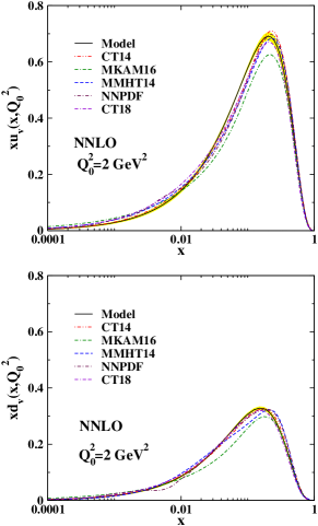
Figure 1: (Color online) The up and down valence parton distributions $xu_{v}$ and $xd_{v}$ in NNLO accuracy with $\Delta\chi^{2}=1$ uncertainty bands at the initial scale $Q_{0}^{2}=2$ $GeV^{2}$. The dashed-dashed-dotted curve stands for the MKAM16 model MoosaviNejad:2016ebo , the dashed-dotted one shows the NNPDF model Ball:2012cx , the long-dashed curve refers to the MMHT14 model Harland-Lang:2014zoa , the dashed-dotted-dotted curve shows the CT14 model Dulat:2015mca and the dashed-dashed-dotted curve represents the CT18 model Hou:2019efy .

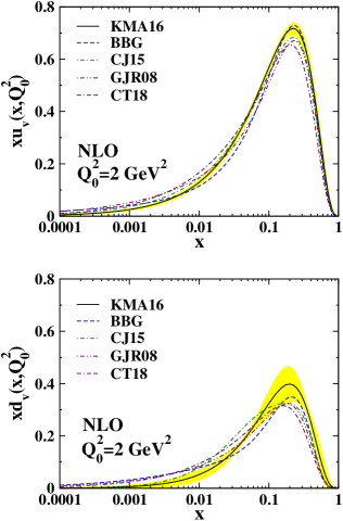
Figure 2: (Color online) The parton densities $xu_{v}$ and $xd_{v}$ in NLO accuracy at the input scale Q${}^{2}_{0}=2\,{\rm GeV}^{2}$. The solid line is the KMA16 PDF Khanpour:2016uxh , dashed line is the BBG PDF Blumlein:2006be , the dashed-dotted line is the CJ15 PDF Accardi:2016qay , dashed-double-dotted line is the GJR08 PDF Gluck:2008gs and dashed-dashed-dotted line shows the result from CT18 model Hou:2019efy .

IV Global analyses of valence-quarks densities

IV.1 Different features of data sets

The valence PDFs can be determined by fitting to a global data set over 572 data points including a variety range of scattering processes at high energies. In Table. 3, the data sets used in our analysis are listed. The DIS data from BCDMS Benvenuti:1989fm ; Benvenuti:1989rh ; Benvenuti:1989gs and SLAC Whitlow:1991uw as well as NMC Arneodo:1996qe ; Arneodo:1995cq experiments make the required sets. The flavor separation of PDFs at large $x$ is facilitated by these data sets. In our analysis, the DIS data from H1 H1 and ZEUS ZEUS Collaborations are also employed. Additionally, the combined measurements of H1 and ZEUS Collaborations at HERA for the inclusive $e^{\pm}p$ scattering cross sections are applied as the new data sets Aaron:2009aa . For the valence quarks in the region $x\geq 0.3$, we use the data set given for $F_{2}^{p}(x,Q^{2})$ and $F_{2}^{d}(x,Q^{2})$ while for the region $x<0.3$ the data are related to $F_{2}^{\rm NS}(x,Q^{2})=2(F_{2}^{p}(x,Q^{2})-F_{2}^{d}(x,Q^{2}))$.

In order to eliminate the higher twist (HT) effects, it is needed to take different cuts on data sets before analysis. The DIS data cuts are considered for Q${}^{2}>4$ GeV² and on the hadronic mass $W^{2}>12.5$ GeV² which perform the required converge in the concerned kinematic region. For the BCDMS and NMC data sets, additional cuts as $y>0.35$ and $Q^{2}>8$ GeV² should be applied, respectively. Considering the required cuts, we listed in Table. 3 both the required DIS data and the number of data points for each experiment in the fitting process. In the 5^th column of Table. 3, taking the additional cuts the number of reduced data points are presented. Consequently, the number of data points are reduced from 467 to 248 for $F_{2}^{p}(x,Q^{2})$ so that for $F_{2}^{d}(x,Q^{2})$ this reduction is from 232 to 159. At last, for $F_{2}^{\rm NS}(x,Q^{2})$ the number of data points are reduced from 208 to 165.

Table 3: Data sets used in our QCD analysis for (a) $F_{2}^{p}(x,Q^{2})$, (b) $F_{2}^{d}(x,Q^{2})$, and (c) $F_{2}^{\rm NS}(x,Q^{2})$. The name of different data sets as well as the range of $x$ and Q² are given in three first columns. The normalization shifts are also listed in the last column.

Experiment	$x$	Q${}^{2}({\rm GeV}^{2})$	$F_{2}^{p}$	$F_{2}^{p}\leavevmode\nobreak\ {\rm cuts}$	${\cal N}$
BCDMS (100)	0.35–0.75	11.75–75.00	51	29	0.996805
BCDMS (120)	0.35–0.75	13.25–75.00	59	32	0.996805
BCDMS (200)	0.35–0.75	32.50–137.50	50	28	0.997833
BCDMS (280)	0.35–0.75	43.00–230.00	49	26	1.002131
NMC (comb)	0.35–0.50	7.00–65.00	15	14	1.000158
SLAC (comb)	0.30–0.62	7.30–21.39	57	57	1.000714
H1 (hQ2)	0.40–0.65	200–30000	26	26	1.001000
ZEUS (hQ2)	0.40–0.65	650–30000	15	15	0.999929
H1 (comb)	0.40–0.65	90–30000	145	21	0.999947
proton			467	248

(a) $F_{2}^{p}(x,Q^{2})$ data points Benvenuti:1989fm ; Benvenuti:1989rh ; Benvenuti:1989gs ; Whitlow:1991uw ; Arneodo:1996qe ; Arneodo:1995cq ; H1 ; ZEUS ; Aaron:2009aa .
Experiment $x$ Q${}^{2}({\rm GeV}^{2})$ $F_{2}^{d}$ $F_{2}^{d}\leavevmode\nobreak\ {\rm cuts}$ ${\cal N}$ BCDMS (120) 0.35–0.75 13.25–99.00 59 32 1.007303 BCDMS (200) 0.35–0.75 32.50–137.50 50 28 1.001829 BCDMS (280) 0.35–0.75 43.00–230.00 49 26 1.001742 NMC (comb) 0.35–0.50 7.00–65.00 15 14 0.998725 SLAC (comb) 0.30–0.62 10.00–21.40 59 59 0.997742 deuteron 232 159
(b) $F_{2}^{d}(x,Q^{2})$ data points Benvenuti:1989fm ; Whitlow:1991uw ; Arneodo:1996qe ; Arneodo:1995cq .
Experiment $x$ Q${}^{2}({\rm GeV}^{2})$ $F_{2}^{\rm NS}$ $F_{2}^{\rm NS}\leavevmode\nobreak\ {\rm cuts}$ ${\cal N}$ BCDMS (120) 0.070–0.275 8.75–43.00 36 30 0.998751 BCDMS (200) 0.070–0.275 17.00–75.00 29 28 0.998758 BCDMS (280) 0.100–0.275 32.50–115.50 27 26 0.999529 NMC (comb) 0.013–0.275 4.50–65.00 88 53 1.000135 SLAC (comb) 0.153–0.293 4.18–5.50 28 28 1.000923 non-singlet 208 165
(c) $F_{2}^{\rm NS}(x,Q^{2})$ data points Benvenuti:1989fm ; Whitlow:1991uw ; Arneodo:1996qe ; Arneodo:1995cq .

IV.2 $\chi^{2}$-Minimization approach

The best values of fit parameters at NNLO accuracy are extracted by minimizing the $\chi^{2}$ with respect to four unknown parameters in valence-quark distributions (14) and (15), along with $\Lambda_{\rm{\overline{MS}}}^{(4)}$ as the QCD cutoff parameter. As is shown in Tables. 1 and 2, we fix four parameters in the fit from the beginning, i.e. $\gamma_{u},\eta_{u},\gamma_{d}$ and $\eta_{d}$, so there are totally five free parameters remaining to be extracted from the fit process.
The global goodness-of-fit can be done using the following definition for the effective $\chi^{2}$ cor

$$\chi_{\mathrm{global}}^{2}=\sum_{n}w_{n}\chi_{n}^{2}\;,$$ (24)

where, $n$ labels the different experiments and

$$\chi_{n}^{2}=\left(\frac{1-{\cal N}_{n}}{\Delta{\cal N}_{n}}\right)^{2}+\sum_{i}\left(\frac{{\cal N}_{n}F_{2,i}^{data}-F_{2,i}^{theor}}{{\cal N}_{n}\Delta F_{2,i}^{data}}\right)^{2}.$$ (25)

In the above relation, $F_{2,i}^{data}$, $\Delta F_{2,i}^{data}$ and $F_{2,i}^{theor}$ stand for the data value, the data uncertainty including a combination of statistical and systematic errors, and the theoretical value for the $i^{\mathrm{th}}$ data point in the $n^{\mathrm{th}}$ experiment, respectively. Moreover, ${\Delta{\cal N}_{n}}$ in the first parenthesis is the experimental normalization uncertainty and for the data of $n^{\mathrm{th}}$ experiment an overall normalization factor is given by ${\cal N}_{n}$. This factor is extracted through the fit procedure and when it is determined through the first fit we fix its value in next stages. The possible weighting factor denotes by $w_{n}$ which is usually taken to be 1. In our analysis, a relative normalization shift between the different data sets, i.e., ${\cal N}_{n}$, is used for which the normalization uncertainties ${\Delta{\cal N}_{n}}$ are given by the experiments.

In our analysis, the total number of data points are $n^{data}=572$ and there are also five unknown parameters in the fit. The best parametrization of valence-quark densities are obtained using the CERN program library MINUIT CERN-Minuit . The results are listed in Tables. 1 and 2.

IV.3 Determining the input uncertainties

In this subsection, we describe our method to determine the uncertainties of valence-quark PDFs as well as the error propagation from experimental data points. In practice, the uncertainties in global PDF analysis can be achieved by procedures which are well-defined to propagate through the experimental uncertainties on the fitted data points to the PDF uncertainties. For this purpose, we apply the Hessian method (or error matrix approach) Pumplin:2001ct which is based linearly on error propagation and the suitable production of PDF eigenvector. The Hessian method was firstly used in analysis by MRST04 Martin:2003sk , MSTW08 Martin:2009iq , MRST03 Martin:2002aw , CETQ group Dulat:2015mca and its up-to-dated version by CT18 Hou:2019efy , and also in our previous works AtashbarTehrani:2012xh ; Khanpour:2016pph ; Monfared:2011xf ; Khanpour:2012tk . By running the CERN program library MINUIT CERN-Minuit , an error analysis can be done using the Hessian matrix. A simple and efficient method to calculate the uncertainties of parton densities can be obtained by applying this method which is essentially related to diagonalize the covariance matrix. In the Hessian approach, the main assumption is to perform a quadratic expansion of $\chi^{2}_{\text{ global}}$ with respect to the fitted parameters $a_{i}$ about its global minimum. It reads

$$\Delta\chi^{2}\equiv\chi^{2}_{\text{global}}-\chi^{2}_{\text{m}in}=\sum_{\text{ i, j=1}}^{p}(a_{i}-a_{i}^{0})\,H_{\rm ij}\,(a_{j}-a_{j}^{0})\;.$$ (26)

In this equation, the elements of the Hessian matrix are denoted by $H_{\rm ij}$ and the number of parameters in the global fit is presented by $p$.

IV.4 Error calculations

The method presented in Refs. Martin:2002aw ; Martin:2003sk ; Pumplin:2001ct ; Martin:2009iq ; AtashbarTehrani:2012xh ; Khanpour:2016pph can be followed to determine the error of calculations. The eigenvectors and eigenvalues of the covariance (or Hessian) matrix are the basic mathematical tools. For practical purposes we need, at first, to have a set of appropriate fit parameters considered in the valence quark densities. They are usually labeled by $a_{i}(s_{\text{min}})$ and required to minimize the $\chi^{2}_{\text{ global}}$. Considering the parton sets as $s_{k}^{\pm}$, it is possible to have an expansion in terms of the eigenvectors and eigenvalues for the variation of parameters around the global minimum, i.e.

$$a_{i}(s_{k}^{\pm})=a_{i}(s_{\text{min}})\pm t\sqrt{\lambda_{k}}v_{\text{ik}}\;.$$ (27)

Here, $a_{i}(s_{k}^{\pm})$ and $a_{i}(s_{\text{min}})$ are the same as the abbreviated $a_{i}$ and $a_{i}^{0}$ symbols in Eq. (26). In the above equation, the k${}^{\text{th}}$-eigenvalue and the i${}^{\text{th}}$-component of the orthonormal eigenvectors of Hessian matrix are denoted by $\lambda_{k}$ and $v_{\text{ik}}$, respectively. By adjusting the $t$ variable proportionally, it is possible to set $t=T$ in the quadratic approximation and therefore to get $T^{2}=\Delta\chi^{2}$. The quadratic approximation of Eq. (26) can be tested by considering the dependence of $\Delta\chi^{2}$ on the eigenvector directions for some selected samples. In Fig. 3, $\Delta\chi^{2}$ is plotted as a function of $t$ for all eigenvectors at the NNLO accuracy.

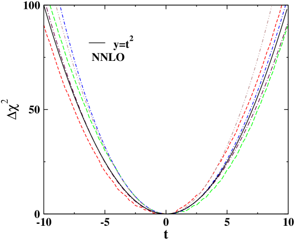
Figure 3: (Color online) $\Delta\chi^{2}$ as a function of $t$ at NNLO accuracy Khanpour:2016pph ; AtashbarTehrani:2012xh ; Martin:2002aw ; Pumplin:2001ct ; Martin:2003sk ; Martin:2009iq . The indicated curves correspond to all five eigenvectors.

	$\alpha_{u_{v}}$	$\beta_{u_{v}}$	$\alpha_{d_{v}}$	$\beta_{d_{v}}$	$\Lambda_{\overline{\rm MS}}^{(4)}$
$\alpha_{u_{v}}$	1
$\beta_{u_{v}}$	0.0957708	1
$\alpha_{d_{v}}$	-0.0500717	-0.294017	1
$\beta_{d_{v}}$	-0.0315322	-0.23711	0.910278	1
$\Lambda_{\overline{\rm MS}}^{(2)}$	0.0445004	-0.585629	-0.0247452	-0.127968	1

Table 4: The correlation matrix elements for the 4 + 1 free parameters at NNLO fit.

In our NNLO global analysis, the covariance matrix elements for five free parameters are given in Table. 4. The estimation for uncertainties of parton densities which is generally denoted by $F$ can be determined, using the following relation introduced in Martin:2002aw :

$$(\Delta F)^{2}=\Delta\chi^{2}\sum_{i=1}^{p}\sum_{j=1}^{p}\frac{\partial F}{\partial a_{i}}C_{ij}(a)\frac{\partial F}{\partial a_{i}},$$ (28)

where, $C_{ij}(a)=(H^{-1})_{ij}$ is the covariance matrix and $\Delta\chi^{2}$ is the allowed variation in $\chi^{2}$, as was specified previously. By suitable choice of $\Delta\chi^{2}=1$, which corresponds to one sigma confidence level, and by considering the Hessian (or equivalently covariance) matrix it is now possible to calculate the errors on parton densities.

Now, the valence quark densities can be calculated at higher-Q² (i.e. $Q^{2}>Q_{0}^{2}$) using the DGLAP evolution equations in Laplace $s$-space. Using the analytical solution, based on the Laplace transform technique as well as Jacobi polynomials approach, the global QCD analysis can be done. In Table. 1, we listed the numerical values of PDFs parameters which are related to the QCD fit for the NNLO non-singlet sector at the input scale Q${}_{0}^{2}=2$ GeV². After the first minimization, some parameters take values with very small error so that one can ignore their errors and fix them to their central values through the fit procedure. By fixing some parameters, the fit is repeated which could be done easier and faster. Hence some parameters are presented in Tables. 1 and 2 without any error. We can see from Table. 1 that the central values of PDF parameters are rather stable. From the fit, one can find the numerical value for $\alpha_{\rm s}^{\rm N_{f}=4}(Q_{0}^{2})$ as presented in Tables. 1 and 2. This implies the numerical value for QCD cutoff quantity. Using this quantity and considering the threshold matching condition for running coupling constant match , we get $\alpha_{s}(M_{Z}^{2})=0.1147\pm 0.0009$ at the mass scale of $Z$-boson. In Fig. 1, we depicted the $xu_{v}$- and $xd_{v}$-distributions at the energy scale $Q_{0}^{2}=2$ GeV². This also contains the PDF uncertainties with required confidence level corresponding to $\Delta\chi^{2}=1$ in Eq. (26). In this figure, we have also added the results from other models such MKAM16 MoosaviNejad:2016ebo , NNPDF Ball:2012cx , MMHT14 Harland-Lang:2014zoa , CT14 Dulat:2015mca and up-to-dated results from CT18 PDFs Hou:2019efy to have a more qualitative comparison. To confirm the considerable progress of PDFs at NNLO accuracy, the results of NLO PDFs for up and down valence densities have been also depicted in Fig. 2 at the scale $Q_{0}^{2}=2$ GeV². The numerical values of fitted parameters at NLO accuracy are listed in Table. 2. As is seen from Tables. 1 and 2, the value of $\chi^{2}/{\rm n.d.f}$ is reduced from 0.920 to 0.906 by increasing the accuracy of corrections from NLO to NNLO. Moreover, in Fig. 2 the small uncertainty raised in our NNLO analysis confirms the validity of NNLO analysis in comparison with the NLO one. Of course, the higher order correction is not the only reason for decreasing the errors and additionally the type of fitting procedure would be also effective on getting the small error bands. This point will be described in the following section.

V Higher twist and target mass corrections

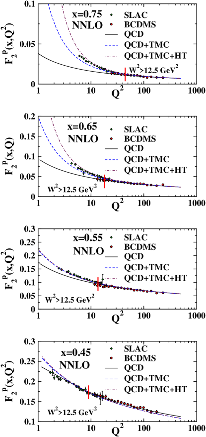
Figure 4: (Color online) Comparison of data for proton structure function ($F^{p}_{2}$) from BCDMS Benvenuti:1989fm ; Benvenuti:1989rh ; Benvenuti:1989gs and SLAC Whitlow:1991uw , with our theoretical predictions as a function of Q² for fixed values of $x$. This plot includes, the pure QCD fit at NNLO (solid line), the TMCs contributions (dashed line), and the HT effect (dashed-dotted line).

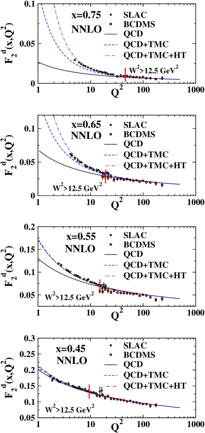
Figure 5: (Color online) As in Fig. 4, but for deuteron structure function ($F^{d}_{2}$). In this figure as well as Fig. 4, to extract the PDFs parameters through the fit we just used the data points after the vertical red lines. These data points belong to the region $W^{2}\geq 12.5\;GeV^{2}$.

To determine the moment of structure function, it is assumed that in the limit of $Q^{2}\rightarrow\infty$ the mass of target hadron approaches to zero. This assumption would be violated at the intermediate and low values of $Q^{2}$. In these regions, the moment is significantly affected by the power correction of order ${\cal O}(m_{N}^{2}/Q^{2})$ where $m_{N}$ denotes the nucleon mass Kataev:1996vu ; Kataev:1997nc . This correction is known as the target mass correction (TMC). Taking into account the TMC effect leads to change the moment of non-singlet structure function as it follows  Khorramian:2008yh ; Khorramian:2009xz ; Khanpour:2016uxh ; Georgi:1976ve ; Gluck:2006yz ; Steffens:2012jx ,

$${\cal M}_{2,{\rm TMC}}^{k}(s,Q^{2})\equiv{\cal L}[{\cal M}_{2,{\rm TMC}}^{k}(e^{-v},Q^{2};s)]\,$$

$$={\cal M}_{2}^{k}(s,Q^{2})+\frac{s(s-1)}{s+2}\left(\frac{m_{N}^{2}}{Q^{2}}\right)\,{\cal M}_{2}^{k}(s+2,Q^{2})$$

$$+\frac{\Gamma(s+3)^{2}}{2\Gamma(s-1)\Gamma(s+5)}\left(\frac{m_{N}^{2}}{Q^{2}}\right)^{2}\,{\cal M}_{2}^{k}(s+4,Q^{2})$$

$$+\frac{\Gamma(s+4)\Gamma(s+5)}{6\Gamma(s-1)\Gamma(s+7)}\left(\frac{m_{N}^{2}}{Q^{2}}\right)^{3}\,{\cal M}_{2}^{k}(s+6,Q^{2})$$

$$+\frac{\Gamma(s+5)\Gamma(s+7)}{24\Gamma(s-1)\Gamma(s+9)}\left(\frac{m_{N}^{2}}{Q^{2}}\right)^{4}\,{\cal M}_{2}^{k}(s+8,Q^{2})$$

$$+{\cal{O}}\left(\frac{m_{N}^{2}}{Q^{2}}\right)^{5}\;.$$ (29)

In the relevant region where $x<0.8$, the higher powers of $(m_{\rm N}^{2}/Q^{2})^{n}$ (for $n\geqslant 2$) are negligible Georgi:1976ve . By substituting Eq. (V) into Eq. (III), one obtains

$$F_{2}^{k,{\rm TMC}}(x,Q^{2}) = x^{\beta}(1-x)^{\alpha}\sum_{n=0}^{\rm N_{max}}\Theta_{n}^{\alpha,\beta}(x)$$

$$\times \sum_{j=0}^{n}\,c_{j}^{(n)}{(\alpha,\beta)}\,{\cal M}_{2,{\rm TMC}}^{k}(j+1,Q^{2})\,,$$

where, ${\cal M}_{2,{\rm TMC}}^{k}(j+1,Q^{2})$ is the moment of concerned structure function in the Laplace $s$-space. This term contains the TMC effect and is given by Eq. (V) where the corrections due to higher powers (for $n\geqslant 2$) are neglected.

The effect of higher twist (HT) correction is also significant at large values of $x$ and moderate $Q^{2}$ Abt:2016vjh ; Jimenez-Delgado:2013boa ; Leader:2006xc ; Nath:2016phi ; Wei:2016far where the TMC effect is also considerable. Consequently, inclusion of higher twists has its own importance to analysis the parton densities.

The required kinematic cuts, containing the HT effect for $F_{2}^{p}(x,Q^{2})$ and $F_{2}^{d}(x,Q^{2})$, are as $Q^{2}\geq 4$ GeV² and $W^{2}\geq 12.5$ GeV² where $W^{2}$ denotes the hadronic invariant mass. The cuts can be extended to the kinematic region $4<W^{2}<12.5{\rm GeV}^{2}$. Therefore, an extrapolation is needed to this region in our QCD fit. It should be noted that, the $W^{2}$ is related to the $Q^{2}$-variable through $W^{2}=(1/x-1)Q^{2}+m^{2}_{n}$, where $m_{n}$ is the nucleon mass. From this relation, it can be seen that the required kinematic cut is such that for $W^{2}\geq 12.5$ GeV², the $Q^{2}$ is also increasing. Consequently, the TMC and HT effects can be ignored in this region. Therefore, as is seen from Figs. 4 and 5, three plots labeled as QCD, QCD+TMC and QCD+TMC+HT show the same behavior.

Concerning the higher twist effect it should be noted that, the parametrization form of higher twist contributions are practically independent of the leading twist one. This parametrization is typically given by polynomial functions of $x$. For the DIS data where the power corrections in the concerned region can not be neglected, the corrections are defined by an ansatz which is completely motivated from phenomenological points of view and it reads Blumlein:2008kz ; Blumlein:2006be ; Martin:1998np ; Martin:2003sk

$$F_{2}^{\rm HT}(x,Q^{2})={\cal O}_{\rm TMC}[F_{2}^{\rm TMC}(x,Q^{2})]\left(1+\frac{h(x,Q^{2})}{Q^{2}[{\rm GeV}^{2}]}\right)\,,$$

where $F_{2}^{\rm TMC}(x,Q^{2})$ is given by Eq. (V). The operation ${\cal O}_{\rm TMC}[\cdots]$ in the above equation refers to the target mass correction while the twist-2 contribution is considered for the desired structure function. It should be noted that, the $h(x,Q^{2})$-coefficient is determined at individual intervals of $x$ and Q² but finally the averaged result over Q² is taken into account. Therefore, the $x$-dependence of $h(x)$ as the higher twist contribution could be defined as Blumlein:2008kz

$$h(x)=\alpha\left(\frac{x^{\beta}}{1-x}-\gamma\right)\,.$$ (32)

To achieve a flexible higher twist contribution during the data analysis, the above choice of $h(x,Q^{2})$ would be effective. As was mentioned, the cuts $Q^{2}\geq 4\,{\rm GeV}^{2}$ and $4<W^{2}<12.5\,{\rm GeV}^{2}$ should be considered for the higher twist QCD analysis of the non-singlet data. The value of $\Lambda_{\rm QCD}$ and the free parameters of valence PDFs and function $h(x)$ could be extracted through the fit procedure to all available data. Our strategy is to perform a fit for the PDF parameters at large values of $W^{2}$ and then to impose the TMC effect to the structure functions. Following that a HT-term is added to the calculation while the PDFs parameters are fixed. The free parameters of HT-term are determined during the second stage of fit procedure using the lower values of $W^{2}$. Our reason for this strategy of fitting is to indicate the ability of Laplace transformation technique at the NNLO expansion to extract the non-singlet structure function. The fitted result for the HT term is listed in Table. 5.

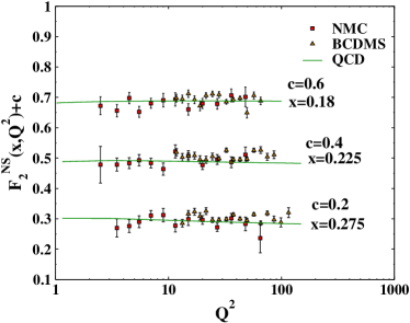
Figure 6: (Color online) Comparison of our NNLO QCD predictions for the non-singlet structure function ($F^{\rm NS}_{2}$) with the dara from BCDMS and NMC Arneodo:1996qe ; Arneodo:1995cq .

NNLO
$h(x)$	$\alpha=1.07092$	$\beta=0.842737$	$\gamma=1.12905$

Table 5: The values of HT parameters in Eq. (32) extracted through the NNLO fit at Q${}_{0}^{2}=2\,{\rm GeV}^{2}$.

VI Results and Discussion

In this work, we discussed about the results arising from the PDF fits. In this regard, we analyzed the global fitting on parton densities in Sec. IV. They are mostly related to Figs. 1, 2 and 3 and also to the corresponding Tables. 1, 2 and 4. In Fig. 3, we indicated the results of $\Delta\chi^{2}$ with respect to the $t$-variable considering all five eigenvectors. As can be seen, a very good description of data is provided by considering our theoretical predictions which are based on the analytical solutions resulted from the Laplace transform technique and Jacobi polynomials approach.

The rest of results are related to the TMC and HT effects which have been described in Sec. V, in detail. In this section, Fig. 4 involves the data for inclusive proton structure functions ($F_{2}^{p}$) from BCDMS and SLAC experiments. A comparison between available experimental data and our NNLO fit, as a function of Q² at approximately constant values of $x$, has been also done. The effects of TMC and HT corrections have been also included so that a considerable agreement between the experimental data and the theoretical predictions is achieved especially at low energy scales. Briefly, our strategy includes two steps. In the first step, we performed the required analysis to get the best values for the PDF parameters. At the second step, the TMC and HT effects have been included. They affected the results, specially at low energy scales. Final results, which are shown in Figs. 4 and 5, indicate good agreements with the experimental data for the available range of energy scales. A more detailed comparison between the theoretical predictions of our NNLO fit and the data for the deuteron structure function ($F^{d}_{2}$) has been depicted in Fig. 5. The results have contained again the effect of TMC and HT corrections.

In Fig. 6, a comparison between the structure function for $(d-p)$, i.e. $F^{\rm NS}_{2}$, and the data from BCDMS and NMC experiments has been shown. For better presentation, the data have been scaled by $c=0.2$, $c=0.4$ and $c=0.6$ for $x=0.275$, $x=0.225$ and $x=0.18$, respectively.

Here, we just remind that the agreement between the theoretical predictions and the experimental data becomes significantly better when one employs the effect of TMC and HT corrections. This point can be seen clearly in Figs. 4 and 5. In this regard, we have also got an excellent agreement between the theoretical prediction for the structure functions $F^{p}_{2}$ and $F^{d}_{2}$ and the available experimental data which included the TMC and HT effects. The data included different ranges of Q² and $x$-values.
The technique of Laplace transformation can be also employed in analyzing the Drell-Yan data which contain antiquark distributions. This type of distribution has not been yet considered in our recent analysis. It would be also valuable if we can improve the method of our fitting by including the TMC calculation and the parameters of HT term together with the PDF parameters, simultaneously. These projects are in progress and remain as our future works.

Appendix A

In this appendix, we present the Laplace transforms for the NLO and NNLO splitting functions as well as the Wilson coefficient functions. They are related to the non-singlet sectors of structure function used in Eq. (6) and Eqs. (III)-(III). In deriving the NLO and NNLO Wilson coefficients $C_{2NS}^{(1)}$ and $C_{2NS}^{(2)}$ in Laplace $s$-space, we use the corresponding results at $x$-space given in Refs. Moch:1999eb ; Vermaseren:2005qc . The NLO and NNLO splitting functions in $s$-space, i.e. $\Phi_{(NS)}^{\rm NLO}$ and $\Phi_{(NS)}^{\rm NNLO}$, are calculated from the corresponding results in $x$-space which are given in Refs. Curci:1980uw ; Moch:2004pa . The obtained results for splitting functions and the Wilson coefficients in $s$-space are as following:

$$\Phi_{\rm{NS}}^{\rm{NLO}}=\hskip 398.33858pt\text{(A.1)}$$

$$C_{F}T_{F}\left(-\frac{2}{3(1+s)^{2}}-\frac{2}{9(1+s)}-\frac{2}{3(2+s)^{2}}+\frac{22}{9(2+s)}+\frac{20\left(\gamma_{E}+\psi(s+1)\right)}{9}+\frac{4}{3}\psi^{\prime}(s+1)\right)+$$

$$C_{F}{}^{2}\left(-\frac{1}{(1+s)^{3}}-\frac{5}{1+s}-\frac{1}{(2+s)^{3}}+\frac{2}{(2+s)^{2}}+\frac{5}{2+s}+\right.$$

$$\frac{2\left(\gamma_{E}+\frac{1}{1+s}+\psi(s+1)-(1+s)\psi^{\prime}(s+2)\right)}{(1+s)^{2}}+\frac{2\left(\gamma_{E}+\frac{1}{2+s}+\psi(s+2)-(2+s)\psi^{\prime}(s+3)\right)}{(2+s)^{2}}-$$

$$\left.4\left(\left(\gamma_{E}+\psi(s+1)\right)\psi^{\prime}(s+1)-\frac{1}{2}\psi^{\prime\prime}(s+1)\right)+3\psi^{\prime}(s+1)\right)+$$

$$C_{A}C_{F}\left(-\frac{1}{(1+s)^{3}}+\frac{5}{6(1+s)^{2}}+\frac{53}{18(1+s)}+\frac{\pi^{2}}{6(1+s)}-\frac{1}{(2+s)^{3}}+\right.$$

$$\frac{5}{6(2+s)^{2}}-\frac{187}{18(2+s)}+\frac{\pi^{2}}{6(2+s)}-\frac{67\left(\gamma_{E}+\psi(s+1)\right)}{9}+$$

$$\left.\frac{1}{3}\pi^{2}\left(\gamma_{E}+\psi(s+1)\right)-\frac{11}{3}\psi^{\prime}(s+1)-\psi^{\prime\prime}(s+1)\right)\,,$$

$$C_{2NS}^{(1)}(s)=\hskip 398.33858pt\text{(A.2)}$$

$$C_{F}\left(-9-\frac{2\pi^{2}}{3}-\frac{2}{(1+s)^{2}}+\frac{6}{1+s}-\frac{2}{(2+s)^{2}}+\frac{4}{2+s}+3\left(\gamma_{E}+\psi(s+1)\right)+\right.$$

$$\frac{2\left(\gamma_{E}+\psi(s+2)\right)}{1+s}+\frac{2\left(\gamma_{E}+\psi(s+3)\right)}{2+s}+$$

$$\left.\frac{1}{3}\left(\pi^{2}+6\left(\gamma_{E}+\psi(s+1)\right){}^{2}-6\psi^{\prime}(s+1)\right)+4\psi^{\prime}(s+1)\right)\,,$$

$$\Phi_{\text{NS}}^{\text{NNLO}}\hskip 398.33858pt\text{(A.3)}$$

$$=1295.384+\frac{1024}{27(1+s)^{5}}-\frac{1600}{9(1+s)^{4}}+\frac{589.8}{(1+s)^{3}}-\frac{1258}{(1+s)^{2}}+\frac{1641.1}{1+s}-\frac{3135}{2+s}+$$

$$\frac{243.6}{3+s}-\frac{522.1}{4+s}-1174.898\left(\gamma_{E}+\psi(1+s)\right)-\frac{714.1\left(\gamma_{E}+\psi(2+s)\right)}{1+s}+$$

$$\frac{563.9}{(1+s)^{2}}\left(\gamma_{E}+\frac{1}{1+s}+\psi(1+s)-(1+s)\psi^{\prime}(2+s)\right)+$$

$$f\left(173.927+\frac{128}{9(1+s)^{4}}-\frac{5216}{81(1+s)^{3}}+\frac{152.6}{(1+s)^{2}}-\frac{197}{1+s}+\frac{8.982}{(2+s)^{4}}+\frac{381.1}{2+s}+\frac{72.94}{3+s}+\right.$$

$$\frac{44.79}{4+s}+183.187\left(\gamma_{E}+\psi(1+s)\right)+\frac{5120\left(\gamma_{E}+\psi(2+s)\right)}{81(1+s)}-$$

$$\left.\frac{56.66}{(1+s)^{2}}\left(\gamma_{E}+\frac{1}{1+s}+\psi(1+s)-(1+s)\psi^{\prime}(2+s)\right)\right)-$$

$$\frac{256.8}{(1+s)^{4}}\left(3+2\gamma_{E}(1+s)+2\gamma_{E}(1+s)^{2}\psi(1+s)-(1+s)\left(-1+2\gamma_{E}(1+s)\right)\psi(1+s)+\right.$$

$$(1+s)^{3}\psi(1+s)^{2}\psi(2+s)-2(1+s)^{3}\psi(1+s)\psi(2+s)^{2}+(1+s)^{3}\psi(2+s)^{3}-$$

$$\left.2(1+s)^{2}\psi^{\prime}(1+s)+(1+s)^{3}\psi\text{''}(2+s)\right)+$$

$$f^{2}\left(\frac{64\left(\gamma_{E}+\psi(1+s)\right)}{81}+\right.$$

$$\frac{64}{81}\left(-\frac{51}{16}+\frac{5\pi^{2}}{6}+\frac{3}{2(1+s)^{3}}-\frac{11}{2(1+s)^{2}}+\frac{7}{1+s}-\frac{3}{2(2+s)^{3}}+\frac{11}{2(2+s)^{2}}-\frac{6}{2+s}-\right.$$

$$\left.\left.3\zeta(3)-5\psi^{\prime}(2+s)-\frac{3}{2}\psi\text{''}(2+s)\right)\right)$$

$$C_{2\text{NS}}^{(2)}=\hskip 398.33858pt\text{(A.4)}$$

$$-338.513+\frac{160}{9(1+s)^{4}}-\frac{41.4}{(1+s)^{3}}+\frac{28.384}{(1+s)^{2}}-\frac{181}{1+s}+\frac{17.256}{(2+s)^{5}}-\frac{806.7}{2+s}-$$

$$188.641\left(\gamma_{E}+\psi(1+s)\right)+\frac{628.8\left(\gamma_{E}+\psi(2+s)\right)}{1+s}-$$

$$2.5921\left(\pi^{2}+6\left(\gamma_{E}+\psi(1+s)\right){}^{2}-6\psi^{\prime}(1+s)\right)+$$

$$\frac{72.24\left(\pi^{2}+6\left(\gamma_{E}+\psi(2+s)\right){}^{2}-6\psi^{\prime}(2+s)\right)}{6+6s}+$$

$$\frac{24.5166}{(1+s)^{2}}\left(6\gamma_{E}{}^{2}+\pi^{2}+\frac{12\gamma_{E}}{1+s}+12\gamma_{E}\psi(1+s)-6(1+s)\psi(1+s)\psi(2+s)^{2}+\right.$$

$$6(1+s)\psi(2+s)^{3}-6\left(3+2\gamma_{E}(1+s)\right)\psi^{\prime}(2+s)-12(1+s)\psi(1+s)\psi^{\prime}(2+s)+$$

$$6(1+s)\psi\text{''}(2+s))-$$

$$\frac{37.75}{(1+s)^{4}}\left(3+2\gamma_{E}(1+s)+2\gamma_{E}(1+s)^{2}\psi(1+s)-(1+s)\left(-1+2\gamma_{E}(1+s)\right)\psi(1+s)+\right.$$

$$(1+s)^{3}\psi(1+s)^{2}\psi(2+s)-2(1+s)^{3}\psi(1+s)\psi(2+s)^{2}+(1+s)^{3}\psi(2+s)^{3}-\allowdisplaybreaks[1]$$

$$\left.2(1+s)^{2}\psi^{\prime}(1+s)+(1+s)^{3}\psi\text{''}(2+s)\right)+$$

$$f\left(46.8531+\frac{40}{9(1+s)^{3}}-\frac{16}{3(1+s)^{2}}-\frac{7.8109}{1+s}+\frac{1.1099}{(2+s)^{4}}-\frac{17.82}{2+s}-\frac{12.97}{3+s}-\right.$$

$$6.34888\left(\gamma_{E}+\psi(1+s)\right)-\frac{24.87\left(\gamma_{E}+\psi(2+s)\right)}{1+s}-$$

$$\frac{58}{81}\left(\pi^{2}+6\left(\gamma_{E}+\psi(1+s)\right){}^{2}-6\psi^{\prime}(1+s)\right)-\allowdisplaybreaks[1]$$

$$\frac{15\left(\pi^{2}+6\left(\gamma_{E}+\psi(2+s)\right){}^{2}-6\psi^{\prime}(2+s)\right)}{6+6s}+$$

$$\frac{8.113\left(\gamma_{E}+\frac{1}{1+s}+\psi(1+s)-(1+s)\psi^{\prime}(2+s)\right)}{(1+s)^{2}}-$$

$$\frac{8}{27}\left(-2\gamma_{E}{}^{3}-\gamma_{E}\pi^{2}-6\gamma_{E}\psi(1+s)^{2}-2\psi(1+s)^{3}-\right.$$

$$\left.\left.\psi(1+s)\left(6\gamma_{E}{}^{2}+\pi^{2}-6\psi^{\prime}(1+s)\right)+6\gamma_{E}\psi^{\prime}(1+s)-2\psi\text{''}(1+s)-4\zeta(3)\right)\right)+$$

$$\frac{8.87}{1+s}\left(2\gamma_{E}{}^{3}+\gamma_{E}\pi^{2}+6\gamma_{E}\psi(2+s)^{2}+2\psi(2+s)^{3}+\psi(2+s)\left(6\gamma_{E}{}^{2}+\pi^{2}-6\psi^{\prime}(2+s)\right)-\right.$$

$$\left.6\gamma_{E}\psi^{\prime}(2+s)+2\psi\text{''}(2+s)+4\zeta(3)\right)-$$

$$\frac{92}{9}\left(-\left(\gamma_{E}+\psi(1+s)\right)\left(\pi^{2}+2\left(\gamma_{E}+\psi(1+s)\right){}^{2}-6\psi^{\prime}(1+s)\right)-\right.$$

$$2(\psi\text{''}(1+s)+2\zeta(3)))+$$

$$\frac{128}{9}\left(\frac{\gamma_{E}{}^{4}}{4}+\frac{\gamma_{E}{}^{2}\pi^{2}}{4}+\frac{3\pi^{4}}{80}+\gamma_{E}\psi(1+s)^{3}+\frac{1}{4}\psi(1+s)^{4}+\right.$$

$$\frac{1}{4}\psi(1+s)^{2}\left(6\gamma_{E}{}^{2}+\pi^{2}-6\psi^{\prime}(1+s)\right)-\frac{1}{4}\left(6\gamma_{E}{}^{2}+\pi^{2}\right)\psi^{\prime}(1+s)+$$

$$\frac{3}{4}(\psi^{\prime}(1+s))^{2}+\gamma_{E}\psi\text{''}(1+s)-\frac{1}{4}\psi\text{'''}(1+s)+2\gamma_{E}\zeta(3)+$$

$$\left.\psi(1+s)\left(\gamma_{E}{}^{3}+\frac{\gamma_{E}\pi^{2}}{2}-3\gamma_{E}\psi^{\prime}(1+s)+\psi\text{''}(1+s)+2\zeta(3)\right)\right)$$

References

- (1) R. D. Ball et al. [NNPDF Collaboration], “Parton distributions from high-precision collider data,” Eur. Phys. J. C 77, 663 (2017).
- (2) C. Bourrely and J. Soffer, “New developments in the statistical approach of parton distributions: tests and predictions up to LHC energies,” Nucl. Phys. A 941, 307 (2015).
- (3) L. A. Harland-Lang, A. D. Martin, P. Motylinski and R. S. Thorne, “Parton distributions in the LHC era: MMHT 2014 PDFs,” Eur. Phys. J. C 75, 204 (2015).
- (4) T. J. Hou et al., “CT14 Intrinsic Charm Parton Distribution Functions from CTEQ-TEA Global Analysis,” JHEP 1802, 059 (2018).
- (5) S. Alekhin, J. Blümlein, S. Moch and R. Placakyte, “Parton distribution functions, , and heavy-quark masses for LHC Run II,” Phys. Rev. D 96, 014011 (2017).
- (6) H. Khanpour, M. Goharipour and V. Guzey, “Effects of next-to-leading order DGLAP evolution on generalized parton distributions of the proton and deeply virtual Compton scattering at high energy,” Eur. Phys. J. C 78, 7 (2018).
- (7) M. Goharipour, H. Khanpour and V. Guzey, “First global next-to-leading order determination of diffractive parton distribution functions and their uncertainties within the xFitter framework,” Eur. Phys. J. C 78, 309 (2018).
- (8) M. Soleymaninia, M. Goharipour and H. Khanpour, “First global QCD analysis of charged hadron fragmentation functions and their uncertainties at next-to-next-to-leading order,” arXiv:1805.04847 [hep-ph].
- (9) S. M. Moosavi Nejad, “Fragmentation functions of and considering the role of heavy quarkonium spin,” Eur. Phys. J. Plus 130, no.7, 136 (2015).
- (10) S. M. Moosavi Nejad and M. Delpasand, Int. J. Mod. Phys. A 30 (2015) no.32, 1550179
- (11) S. M. Moosavi Nejad, Eur. Phys. J. C 72 (2012) 2224
- (12) S. Shoeibi, F. Taghavi-Shahri, H. Khanpour and K. Javidan, “Phenomenology of leading nucleon production in collisions at HERA in the framework of fracture functions,” Phys. Rev. D 97, 074013 (2018).
- (13) N. Cabibbo and R. Petronzio, “Two Stage Model of Hadron Structure: Parton Distributions and Their Dependence,” Nucl. Phys. B 137, 395 (1978).
- (14) M. Miyama and S. Kumano, “Numerical solution of evolution equations in a brute force method,” Comput. Phys. Commun. 94, 185 (1996).
- (15) M. Hirai, S. Kumano and M. Miyama, “Numerical solution of evolution equations for polarized structure functions,” Comput. Phys. Commun. 108, 38 (1998).
- (16) R. Toldra, “A c++ code to solve the DGLAP equations applied to ultrahigh- energy cosmic rays,” Comput. Phys. Commun. 143, 287 (2002).
- (17) W. Furmanski and R. Petronzio, “A Method of Analyzing the Scaling Violation of Inclusive Spectra in Hard Processes,” Nucl. Phys. B 195, 237 (1982).
- (18) J. Blumlein, M. Klein, G. Ingelman and R. Ruckl, “Testing QCD Scaling Violations in the HERA Energy Range,” Z. Phys. C 45, 501 (1990).
- (19) S. Kumano and J. T. Londergan, “A FORTRAN program for numerical solution of the Altarelli-Parisi equations by the Laguerre method,” Comput. Phys. Commun. 69, 373 (1992).
- (20) R. Kobayashi, M. Konuma and S. Kumano, “FORTRAN program for a numerical solution of the nonsinglet Altarelli-Parisi equation,” Comput. Phys. Commun. 86, 264 (1995).
- (21) A. Ghasempour Nesheli, A. Mirjalili and M. M. Yazdanpanah, “Analyzing the parton densities and constructing the xF3 structure function, using the Laguerre polynomials expansion and Monte Carlo calculations,” Eur. Phys. J. Plus 130, 82 (2015).
- (22) M. Gluck, E. Reya and A. Vogt, “Radiatively generated parton distributions for high-energy collisions,” Z. Phys. C 48, 471 (1990).
- (23) D. Graudenz, M. Hampel, A. Vogt and C. Berger, “The Mellin transform technique for the extraction of the gluon density,” Z. Phys. C 70, 77 (1996).
- (24) J. Blumlein and A. Vogt, “The Evolution of unpolarized singlet structure functions at small x,” Phys. Rev. D 58, 014020 (1998).
- (25) J. Blumlein, “Analytic continuation of Mellin transforms up to two loop order,” Comput. Phys. Commun. 133, 76 (2000).
- (26) M. Stratmann and W. Vogelsang, “Towards a global analysis of polarized parton distributions,” Phys. Rev. D 64, 114007 (2001).
- (27) A. N. Khorramian and S. Atashbar Tehrani, “NNLO QCD contributions to the flavor non-singlet sector of ,” Phys. Rev. D 78, 074019 (2008).
- (28) A. N. Khorramian, H. Khanpour and S. Atashbar Tehrani, “Nonsinglet parton distribution functions from the precise next-to-next-to-next-to leading order QCD fit,” Phys. Rev. D 81, 014013 (2010).
- (29) H. Khanpour, A. Mirjalili and S. Atashbar Tehrani, “Analytic derivation of the next-to-leading order proton structure function based on the Laplace transformation,” Phys. Rev. C 95, 035201 (2017).
- (30) S. M. Moosavi Nejad, H. Khanpour, S. Atashbar Tehrani and M. Mahdavi, “QCD analysis of nucleon structure functions in deep-inelastic neutrino-nucleon scattering: Laplace transform and Jacobi polynomials approach,” Phys. Rev. C 94, 045201 (2016).
- (31) G. R. Boroun and S. Zarrin, “The nonsinglet structure function evolution by Laplace method,” Phys. Atom. Nucl. 78, 1034 (2015).
- (32) Gavin P. Salam and Juan Rojo, “A Higher Order Perturbative Parton Evolution Toolkit (HOPPET),” Compt. Phys. Commum 180, 120 (2009).
- (33) M. Botje, “QCDNUM: Fast QCD Evolution and Convolution,” Compt. Phys. Commum 182, 490 (2011).
- (34) V. Bertone, S. Carrazza, J. Rojo “APFEL: A PDF Evolution Library with QED corrections,” Compt. Phys. Commum 185, 1647 (2014).
- (35) M. M. Block, L. Durand, P. Ha and D. W. McKay, “Decoupling the NLO coupled DGLAP evolution equations: an analytic solution to pQCD,” Eur. Phys. J. C 69, 425 (2010).
- (36) M. M. Block, L. Durand, P. Ha and D. W. McKay, “Applications of the leading-order Dokshitzer-Gribov-Lipatov-Altarelli-Parisi evolution equations to the combined HERA data on deep inelastic scattering,” Phys. Rev. D 84, 094010 (2011).
- (37) M. M. Block, L. Durand, P. Ha and D. W. McKay, “An Analytic solution to LO coupled DGLAP evolution equations: a new pQCD tool,” Phys. Rev. D 83, 054009 (2011).
- (38) M. M. Block, “A New numerical method for obtaining gluon distribution functions , from the proton structure function ,” Eur. Phys. J. C 65, 1 (2010).
- (39) M. M. Block, “Addendum to: ‘A new numerical method for obtaining gluon distribution functions , from the proton structure function .’,” Eur. Phys. J. C 68, 683 (2010).
- (40) G. R. Boroun, S. Zarrin and F. Teimoury, “Decoupling of the DGLAP evolution equations by Laplace method,” Eur. Phys. J. Plus 130, 214 (2015).
- (41) G. R. Boroun and B. Rezaei, “Decoupling of the DGLAP evolution equations at next-to-next-to-leading order (NNLO) at low-x,” Eur. Phys. J. C 73, 2412 (2013).
- (42) M. Zarei, F. Taghavi-Shahri, S. Atashbar Tehrani and M. Sarbishei, “Fragmentation functions of the pion, kaon, and proton in the NLO approximation: Laplace transform approach,” Phys. Rev. D 92, 074046 (2015).
- (43) F. Taghavi-Shahri, S. Atashbar Tehrani and M. Zarei, “Fragmentation functions of neutral mesons and with Laplace transform approach,” Int. J. Mod. Phys. A 31, 1650100 (2016).
- (44) J. Sheibani, A. Mirjalili and S. Atashbar Tehrani, “EMC effect in the next-to-leading order approximation based on the Laplace transformation,” Phys. Rev. C 98, 045211 (2018).
-
(45)
S. Atashbar Tehrani, F. Taghavi-Shahri, A. Mirjalili and M. M. Yazdanpanah,
“NLO analytical solutions to the polarized parton distributions, based on the Laplace transformation,”
Phys. Rev. D 87, 114012 (2013)
Erra:Phys. Rev. D 88, 039902 (2013). - (46) M. Salajegheh, S. M. Moosavi Nejad, M. Nejad, H. Khanpour and S. Atashbar Tehrani, “Analytical approaches to the determination of spin-dependent parton distribution functions at NNLO approximation,” Phys. Rev. C 97, 055201 (2018).
- (47) G. Curci, W. Furmanski and R. Petronzio, “Evolution of Parton Densities Beyond Leading Order: The Nonsinglet Case,” Nucl. Phys. B 175, 27 (1980).
- (48) S. Moch, J. A. M. Vermaseren and A. Vogt, “The Three loop splitting functions in QCD: The Nonsinglet case,” Nucl. Phys. B 688, 101 (2004).
- (49) P. Jimenez-Delgado and E. Reya, “Delineating parton distributions and the strong coupling,” Phys. Rev. D 89, no. 7, 074049 (2014).
- (50) A.C.Benvenuti,D.Bollini,G.Bruni,F.L.Navarria,A.Argento, W.Lohmann,L.Piemontese,J.Strachota,P.Zavada,S.Baranov et al. [BCDMS Collaboration], “A High Statistics Measurement of the Deuteron Structure Functions and R From Deep Inelastic Muon Scattering at High ,” Phys. Lett. B 237, 592 (1990).
- (51) A.C.Benvenuti,D.Bollini,G.Bruni,T.Camporesi,L.Monari, F.L.Navarria,A.Argento,J.Cvach,W.Lohmann,L.Piemontese et al. [BCDMS Collaboration], “A High Statistics Measurement of the Proton Structure Functions and R from Deep Inelastic Muon Scattering at High ,” Phys. Lett. B 223, 485 (1989).
- (52) A.C.Benvenuti,D.Bollini,G.Bruni,F.L.Navarria, W.Lohmann,R.Voss,V.I.Genchev,V.G.Krivokhizhin, R.Lednicky,S.Nemecek et al.[BCDMS Collaboration], “A Comparison of the Structure Functions of the Proton and the Neutron From Deep Inelastic Muon Scattering at High ,” Phys. Lett. B 237, 599 (1990).
- (53) L. W. Whitlow, E. M. Riordan, S. Dasu, S. Rock and A. Bodek, “Precise measurements of the proton and deuteron structure functions from a global analysis of the SLAC deep inelastic electron scattering cross-sections,” Phys. Lett. B 282, 475 (1992).
- (54) M.Arneodo,A.Arvidson,B.Badełek,M.Ballintijn, G.Baum,J.Beaufays,I.G.Bird,P.Björkholm,M.Botje,C.Broggini et al. [New Muon Collaboration], “Measurement of the proton and deuteron structure functions, and , and of the ratio ,” Nucl. Phys. B 483, 3 (1997).
- (55) M.Arneodon,A.Arvidson,B.Badełek,M.Ballintijni,G.Baum, J.Beaufays,I.G.Bird,P.Björkholm,M.Botje,C.Broggini et al. [New Muon Collaboration], “Measurement of the proton and the deuteron structure functions, and ,” Phys. Lett. B 364, 107 (1995).
-
(56)
C. Adloff, V. Andreev, B. Andrieu, T. Anthonis, V. Arkadov, A. Astvatsatourov, I. Ayyaz,
A. Babaev, J. Bähr, P. Baranov et al. [H1 Collaboration],
“Deep-inelastic inclusive e p scattering at low and a determination of
Eur. Phys. J. C 21, 33 (2001).
C. Adloff, V. Andreev, B. Andrieu, T. Anthonis, A. Astvatsatourov, A. Babaev, J. Bähr, P. Baranov, E. Barrelet, W. Bartel1 et al. [H1 Collaboration], “Measurement and QCD analysis of neutral and charged current cross sections Eur. Phys. J. C 30, 1 (2003). -
(57)
J. Breitweg, S. Chekanov, M. Derrick, D. Krakauer, S. Magill, D. Mikunas, B. Musgrave, J. Repond,
R. Stanek, R.L. Talaga et al. [ZEUS Collaboration],
“ZEUS results on the measurement and phenomenology of at low and low
,”
Eur. Phys. J. C 7, 609 (1999).
S. Chekanov, M. Derrick, D. Krakauer, S. Magill, B. Musgrave, A. Pellegrino, J. Repond, R. Stanek, R. Yoshida, M.C.K. Mattingly et al. [ZEUS Collaboration], “Measurement of the neutral current cross section and structure function for deep inelastic e+ p scattering at HERA,” Eur. Phys. J. C 21, 443 (2001). - (58) F. D. Aaron, H. Abramowicz, I. Abt,L. Adamczyk,M. Adamus,M. Al-daya Martin,C. Alexa,V. Andreev,S. Antonelli,P. Antonioli,A. Antonov et al. [H1 and ZEUS Collaborations], “Combined Measurement and QCD Analysis of the Inclusive Scattering Cross Sections at HERA,” JHEP 1001, 109 (2010).
- (59) D. Stump, J. Pumplin, R. Brock, D. Casey, J. Huston, J. Kalk, H.L. Lai and W.K. Tung “Uncertainties of predictions from parton distribution functions, the Lagrange multiplier method,” Phys.Rev. D65, 014012 (2010).
- (60) F. James and M. Roos, “Minuit: A System For Function Minimization And Analysis Of The Parameter Errors And Correlations,” Comput. Phys. Commun. 10, 343 (1975). F. James and M. Roos, Minuit: Function Minimization and Error Analysis, CERN Program Library Long Writeup D506 (1994); F. James and M. Winkler, Minuit User’s Guide: C++ Version (2004).
- (61) J. Pumplin, D. Stump, R. Brock, D. Casey, J. Huston, J. Kalk, H. L. Lai and W. K. Tung, “Uncertainties of predictions from parton distribution functions. 2. The Hessian method,” Phys. Rev. D 65, 014013 (2001)
- (62) A. D. Martin, R. G. Roberts, W. J. Stirling and R. S. Thorne, “Uncertainties of predictions from parton distributions. 2. Theoretical errors,” Eur. Phys. J. C 35, 325 (2004)
- (63) A. D. Martin, W. J. Stirling, R. S. Thorne and G. Watt, “Parton distributions for the LHC,” Eur. Phys. J. C 63, 189 (2009)
- (64) A. D. Martin, R. G. Roberts, W. J. Stirling and R. S. Thorne, “Uncertainties of predictions from parton distributions. 1: Experimental errors,” Eur. Phys. J. C 28, 455 (2003).
- (65) S. Dulat et al., “New parton distribution functions from a global analysis of quantum chromodynamics,” Phys. Rev. D 93, 033006 (2016).
- (66) T. J. Hou et al., “New CTEQ global analysis of quantum chromodynamics with high-precision data from the LHC,” arXiv:1912.10053 [hep-ph]..
- (67) S. Atashbar Tehrani, “Nuclear parton densities and their uncertainties at the next-to-leading order,” Phys. Rev. C 86, 064301 (2012).
- (68) H. Khanpour and S. Atashbar Tehrani, “Global analysis of nuclear parton distribution functions and their uncertainties at next-to-next-to-leading order,” Phys. Rev. D 93, 014026 (2016).
- (69) S. T. Monfared, A. N. Khorramian and S. Atashbar Tehrani, “A Global Analysis of Diffractive Events at HERA,” J. Phys. G 39, 085009 (2012).
- (70) H. Khanpour, A. N. Khorramian and S. Atashbar Tehrani, “New parton distributions in fixed flavour factorization scheme from recent deep-inelastic-scattering data,” J. Phys. G 40, 045002 (2013).
- (71) K. G. Chetyrkin, B. A. Kniehl and M. Steinhauser “Strong coupling constant with flavor thresholds at four loops in the MS scheme,” Phys. Rev. D 79, 2184 (1997).
- (72) R. D. Ball et al., “Parton distributions with LHC data,” Nucl. Phys. B 867, 244 (2013).
- (73) A. L. Kataev, A. V. Kotikov, G. Parente and A. V. Sidorov, “Next to next-to-leading order QCD analysis of the CCFR data for xF3 and F2 structure functions of the deep inelastic neutrino - nucleon scattering”, Phys. Lett. B 388, 179 (1996).
- (74) A. L. Kataev, A. V. Kotikov, G. Parente and A. V. Sidorov, “Next to next-to-leading order QCD analysis of the revised CCFR data for xF3 structure function and the higher twist contributions”, Phys. Lett. B 417, 374 (1998).
- (75) H. Georgi and H. D. Politzer, “Freedom at Moderate Energies: Masses in Color Dynamics,” Phys. Rev. D 14, 1829 (1976).
- (76) M. Gluck, E. Reya and C. Schuck, “Non-singlet QCD analysis of up to NNLO,” Nucl. Phys. B 754, 178 (2006).
- (77) F. M. Steffens, M. D. Brown, W. Melnitchouk and S. Sanches, “Parton distributions in the presence of target mass corrections,” Phys. Rev. C 86, 065208 (2012).
- (78) I. Abt, A. M. Cooper-Sarkar, B. Foster, V. Myronenko, K. Wichmann and M. Wing, “Study of HERA ep data at low Q2 and low and the need for higher-twist corrections to standard perturbative QCD fits,” Phys. Rev. D 94, 034032 (2016).
- (79) P. Jimenez-Delgado, A. Accardi and W. Melnitchouk, “Impact of hadronic and nuclear corrections on global analysis of spin-dependent parton distributions,” Phys. Rev. D 89, 034025 (2014).
- (80) E. Leader, A. V. Sidorov and D. B. Stamenov, “Impact of CLAS and COMPASS data on Polarized Parton Densities and Higher Twist,” Phys. Rev. D 75, 074027 (2007).
- (81) N. M. Nath, A. Mukharjee, M. K. Das and J. K. Sarma, “ Structure Function and Gross-Llewellyn Smith Sum Rule with Nuclear Effect and Higher Twist Correction,” Commun. Theor. Phys. 66, 663 (2016).
- (82) S. y. Wei, Y. k. Song, K. b. Chen and Z. t. Liang, “Twist-4 contributions to semi-inclusive deeply inelastic scatterings with polarized beam and target,” arXiv:1611.08688 [hep-ph].
- (83) J. Blumlein, H. Bottcher and A. Guffanti, “Non-singlet QCD analysis of deep inelastic world data at O(),” Nucl. Phys. B 774, 182 (2007).
- (84) A. Accardi, L. T. Brady, W. Melnitchouk, J. F. Owens and N. Sato, “Constraints on large- parton distributions from new weak boson production and deep-inelastic scattering data,” Phys. Rev. D 93, no. 11, 114017 (2016).
- (85) M. Gluck, P. Jimenez-Delgado, E. Reya and C. Schuck, “On the role of heavy flavour parton distributions at high energy colliders,” Phys. Lett. B 664, 133 (2008).
- (86) J. Blumlein and H. Bottcher, “Higher Twist Contributions to the Structure Functions and at Large x and Higher Orders,” Phys. Lett. B 662, 336 (2008).
- (87) A. D. Martin, R. G. Roberts, W. J. Stirling and R. S. Thorne, “Scheme dependence, leading order and higher twist studies of MRST partons,” Phys. Lett. B 443, 301 (1998)
- (88) S. Moch and J. A. M. Vermaseren, “Deep inelastic structure functions at two loops,” Nucl. Phys. B 573, 853 (2000)
- (89) J. A. M. Vermaseren, A. Vogt and S. Moch, “The Third-order QCD corrections to deep-inelastic scattering by photon exchange,” Nucl. Phys. B 724, 3 (2005)