TURTLE: a C library for an optimistic stepping through a topography

Abstract

TURTLE is a C library providing utilities allowing to navigate through a topography described by a Digital Elevation Model (DEM). The library has been primarily designed for the Monte Carlo transport of particles scattering over medium to long ranges, e.g. atmospheric muons. But, it can also efficiently handle ray tracing problems with very large DEMs ($10^{9}$ nodes or more), e.g. for neutrino simulations. The TURTLE library was built on an optimistic ray tracing algorithm, detailed in the present paper. This algorithm proceeds by trials and errors, approximating the topography within the modelling uncertainties of the DEM data. This allows to traverse a topography in constant time, i.e. independently of the number of grid nodes, and with no added memory. Detailed performance studies are provided by comparison to other ray tracing algorithms and as an application to muon transport in a Monte Carlo simulation.

 

Keywords : Topography  $\cdot$ Ray tracing  $\cdot$ Monte Carlo  $\cdot$ Transport

 

1 Introduction

Monte Carlo (MC) simulations are a key element of many physics experiments. Some transport problems require to propagate particles over tens to hundreds of km, in a complex environment. This is for example the case for muography measurements or for experiments searching extraterrestrial neutrinos. Muography is a particularly complex case since particles might scatter, e.g. by grazing the ground and interacting with surface structures. Accurate Monte Carlo computations require a detailed description of the topography over large distances.

Topography data are provided by a Digital Elevation Model (DEM), which can also be a combination of several DEMs, e.g. with different resolutions. A DEM can represent various information, e.g. the surface above ground structures and the canopy, the ground level, the sea level (geoid undulations) w.r.t. a reference ellipsoid. The elevation data, $z$, are commonly stored over a regular grid in geodetic coordinates (latitude, longitude) or projected coordinates, $(x,y)$, e.g. Universal Transverse Mercator (UTM). Such DEMs generate simple surfaces: $z=f(x,y)$. Note that complex features, e.g. cavities or overhanging cliffs, would map several elevation values to a same projected coordinate, $(x,y)$. By definition, the simple DEMs considered here cannot contain such topologies. Unstructured meshes are neither considered in the following. Elevation values are typically stored using 2 bytes (int16_t) per grid node. Large scale data sets comprise $10^{8}$ to $10^{9}$ nodes resulting in a hundreds of MB to a few GB memory footprint. Due to the Earth curvature, when transformed to the Cartesian laboratory frame of the simulation, the grid nodes are no longer equally spaced. Planarity is lost as well over large distances. For example two nodes at the same elevation above sea level, but distant by 10 km, are actually vertically separated by about 8 m in the laboratory frame.

In MC simulations, a geometry is defined as a collection of closed volumes, bounded by surfaces, and filled with various materials. The transport through the geometry is simulated by discrete steps joining interaction vertices along straight line segments. Each Monte Carlo step involves a ray tracing problem. Ray tracing is a generic geometry problem. For example, it is also encountered when rendering high quality 3D scenes in computer graphics, since it allows to account for physical effects like light reflection and refraction. However, in a MC the ray length can be drastically limited by the physics, as interactions occur with the matter of volumes or with external electromagnetic fields. This leads to changes in the particle direction of propagation, at each interaction vertex, requiring specific ray tracing optimisations. The pseudocode 1 describes a simple transport algorithm in order to guide the following discussion.

Pseudocode 1: Simple Monte Carlo transport algorithm

⬇

Input: $\vec{r},\vec{u}$ % The particle position and direction

begin

% Get the initial volume

volume $\leftarrow\$ volume_at($\vec{r}$)

% Iterate until something happens

while $\ldots$

% Get the step limit from the physics

$\lambda$ $\leftarrow\$ physics_distance(volume, $\vec{r}$, $\ldots$)

% Get the distance to the next volume, or an underestimate

$s$, next $\leftarrow\$ distance_to(volume, $\vec{r}$, $\vec{u}$)

if $s\geq\lambda$ then

% Limit the step according to the physics

$s$ $\leftarrow\$ $\lambda$

else

% Update the volume

if next then

volume $\leftarrow\$ next

else

volume $\leftarrow\$ volume_at($\vec{r}$)

end

end

% Update the particle properties

$\vec{r}$ $\leftarrow\$ $\vec{r}+s\vec{u}$

$\ldots$

end

end

A MC transport engine navigates through the geometry using the pseudocode functions: volume_at and distance_to. The former function returns a reference to the volume at a given position, $\vec{r}$. The latter one provides the distance to the closest boundary surface, along a direction, $\vec{u}$. When volumes are explicitly connected, the next volume can also be returned. Some Monte Carlo engines, like MCNP [1, 2, 3], enforce this when defining the geometry. Otherwise the next volume must be found using the volume_at function. Note that an underestimate for the distance to the next volume can be returned instead of the exact one. The pseudocode expects a reference to the current volume to be returned in this case. Underestimates, independent of the particle direction, can be significantly faster to compute even for usual geometric shapes: cube, sphere, $\ldots$ In the case where the Monte Carlo navigation is limited by the physics, $\lambda<s$ for most steps, then using underestimates may speed up the navigation. This strategy is used by the Geant4 [4, 5, 6] multi-purpose MC package. Geant4 is a popular Monte Carlo engine for particle physics. It was originally designed for modelling the interactions of high energy particles within particle physics detectors. The Geant4 engine is flexible though, and there have been many other applications, e.g. in medical physics or for space radiation studies.

In the following, for the sake of clarity, we consider a simple geometry with only two volumes: the atmosphere and the Earth, separated by a ground surface. The ground surface is usually approximated as a collection of plane facets joining the DEM nodes. Tessellating a regular grid of $n$ nodes with triangles requires approximately two triangles per node in the large $n$ limit. Efficiently building a 3D model for a non parametric volume containing billions of facets is rather involved. One should carefully control the memory overhead, i.e. the extra memory used by the 3D model in addition to the original DEM data. For example, adding a single precision float (32 bits) per node already triples the memory usage. At the same time, the geometry must be smartly organised in order to speed up intersection searches.

A generic optimisation method is to sort geometric shapes (volumes, surfaces, $\ldots$) using a Bounding Volume Hierarchy (BVH). The shapes are organised in a tree structure according to their bounding boxes. The tree is sorted in order to speed up subsequent geometry operations, e.g. computing the intersection of the shapes with a line or with a plane. BVHs are used in 3D modelling for ray tracing or collision detection.

Optimising the MC navigation for volumes bounded by a tessellated surface, or by 3D meshes, is a problem that has been previously investigated, e.g. in Geant4 for medical physics applications. In particular, it was pointed out by Poole et al. [7] that for physics limited navigation, a polyhedral meshing of a volume interior can be more efficient than tessellating its bounding surface. Dividing the interior of a volume in virtual sub-volumes naturally provides fast underestimates of the distance to the next boundary. Unfortunately, this study was done at a time where BVH optimisation was not implemented for tessellated surfaces (G4TessellatedSolid). BVH acceleration (SmartVoxels) was however used for the polyhedral mesh. In recent versions of Geant4 (e.g. 10.5) the VecGeom library [8] can be used to speed up tessellated geometries by using a SIMD optimized BVH, see e.g. M. Gheata [9]). Therefore, the conclusion of Poole et al. [7] could be different today.

For regular DEM grids, the memory overhead due to the geometry modelling can be kept down to zero. The geometry can be fully computed on the fly from the initial elevation data. In the case of a regular polyhedral mesh, there exists a natural alternative to BVH trees with zero memory cost: the nodes connectivity. In this case, the exit facet from a polyhedron determines the next volume on the grid. This allows to traverse the full grid in $\mathcal{O}(\sqrt{n})$ operations, $n$ being the number of nodes. In comparison, a BVH tree could in principle perform the same in $\mathcal{O}(\log(n))$ operations. Nevertheless, the former algorithm costs no extra memory when the grid is regular. It could be more efficient when the navigation is limited by the physics.

In addition to the previous issues, let us point out that approximating a topographic surface with flat triangular facets between the nodes is a poor man solution. Instead, higher degree interpolations could be used. With additional developments one might replace the flat facets by smooth surfaces between the nodes, e.g. splines or NURBS. However, we propose a much simpler and straightforward solution to overcome the discussed issues of memory usage, stepping efficiency and accuracy. This solution is called optimistic algorithm in the following. It implies computing an approximate distance to the next volume, rather than an exact one. The compromise of using an approximate stepping can be motivated by the fact that elevation values provided by a DEM are actually space averages around the node coordinates. The typical accuracies of such models is of the order of 10 cm (see e.g. Mukherjee et al. [10]). The optimistic algorithm is presented in next section 2. It is the baseline of the TURTLE library described in section 3. Test cases are presented in section 4. Those are used in order to tune the optimistic algorithm in section 5. Then, we provide detailed performance studies by comparison to other ray tracing algorithms (section 6) and as an application to muon transport in a Monte Carlo simulation (section 7).

2 The optimistic stepping algorithm

An approximate solution to the ray tracing problem is to proceed by trials and errors. When navigating through the DEM data, a tentative (optimistic) stepping distance is proposed for the topography, at each Monte Carlo step. If the step leads to a ground crossing, the boundary is located with a binary search. The stepping distance is reduced iteratively in order to converge to the boundary within an accuracy of $\epsilon$. If there is no ground crossing the step is accepted. Note that if the initial step length, $s_{0}$, is too long one might overrun some details of the topography of size smaller than $s_{0}$. Consequently, this method has a non-null failure rate. Setting a small enough constant value, e.g. $s_{0}=1\,\mathrm{cm}$, mitigates the risk but is very inefficient.

Yet, in the case of a ground surface described by a DEM, a simple yet efficient guess for the initial stepping distance, $s_{0}$, is:

$$s_{0}=\max\left(\alpha|h_{0}-g_{0}|,\,s_{\mathrm{min}}\right)$$ (1)

where $h_{0}$ is the current altitude of the particle and $g_{0}$ the corresponding ground level, i.e. $|h_{0}-g_{0}|$ is the difference in height w.r.t. the ground. The parameters $\alpha\leq 1$ and $s_{\mathrm{min}}$, in eq. (1), are two tuning factors. Let us call them slope factor and resolution factor in the following.

Note that the altitudes $h_{0}$ and $g_{0}$ in equation 1 are considered in the same local referential, i.e. along the local vertical. This is important for particles propagating over long ranges. It ensures that the algorithm properties are not affected by the Earth curvature. Usually the ground altitude w.r.t. sea level, $g_{0}$, can be directly read from DEMs, given the particle geodetic coordinates, i.e. latitude and longitude. A Monte Carlo would however operate in a fixed Cartesian frame instead, e.g. a geocentric frame. This implies extra computations for transforming the particle coordinates at each step.

Using the guess provided by equation 1 instead of a constant step length can provide impressive speed-up, by several orders of magnitude as shown in section 5, without significant loss of accuracy. The driving idea is that as long as slopes are not too steep, the height w.r.t the ground is a safe estimate of the closest distance to the ground. Reducing the slope factor allows to handle steeper and stepper slopes. Note that setting $\alpha$ below $1$ is not efficient for vertical trajectories. In this case, an improvement to equation 1 could be to vary $\alpha$ depending on the particle direction w.r.t. the local vertical. Yet, in this paper we consider only close to horizontal trajectories. The resolution factor plays the role of a safeguard against numerical errors, e.g. close to a boundary. While the boundary is approached with an accurate binary search, it is departed from using a constant step size, given by the resolution factor.

Below are pseudocode implementations of the volume_at and distance_to functions, using the optimistic algorithm and eq. (1) as initial guess for the step length. A key component of the method is the get_geodetic function. Given a particle position in the laboratory frame, this function computes the altitude and the corresponding ground level with respect to a common reference. This latter data is efficiently extracted from the DEMs, on the fly, i.e. without building a complete model of the ground surface. This is the main purpose of the TURTLE library. As a consequence, a Monte Carlo transport engine may navigate quickly and simply through the topography using the optimistic approach.

Pseudocode 2: Example of volume_at function for an optimistic stepping through topography data

⬇

Input: $\vec{r}$ % The particle position

Function volume_at($\vec{r}$)

$h,g$ $\leftarrow\$ get_geodetic($\vec{r}$)

if $h>g$ then

return above

else

return below

end

end

Pseudocode 5: Example of distance_to function for an optimistic stepping through topography data

⬇

Input: $\vec{r},\vec{u}$ % The particle position and direction

volume % A reference to the current volume

Function distance_to(volume, $\vec{r}$, $\vec{u}$)

% Compute the tentative step length

$h_{0},g_{0}$ $\leftarrow\$   get_geodetic($\vec{r}$)

$s_{0}$ $\leftarrow\$ $\ \max\left(\alpha|h_{0}-g_{0}|,\,s_{\mathrm{min}}\right)$

% Check the tentative position

next $\leftarrow\$ volume_at($\vec{r}+s_{0}\vec{u}$)

if next $\neq$ volume then

% Locate the topography crossing with a binary search

$s_{1}$ $\leftarrow\$ $\ 0$

while $s_{0}-s_{1}>\epsilon$

$s_{2}$ $\leftarrow\$ $\ (s_{0}+s_{1})/2$

volume $\leftarrow\$ volume_at($\vec{r}+s_{2}\vec{u}$)

if volume = next then

$s_{0}$ $\leftarrow\$ $\ s_{2}$

else

$s_{1}$ $\leftarrow\$ $\ s_{2}$

end

end

end

return $s_{0}$, next

end

Note that it would be enough to return the signed distance to the ground, $h-g$, from the get_geodetic function. However, providing the particle and ground altitude allows to extend the algorithm by adding volumes bounded by additional topography surfaces. For example, one can define a seawater volume bounded by $g<h\leq 0$, with altitudes measured w.r.t. the sea level. An atmosphere can be defined on top of that as $\max(g,0)<h<h_{\mathrm{max}}$, with $h_{\mathrm{max}}$ the top of the atmosphere. Similarly one could specify an inner structure of the Earth, e.g. following the Preliminary Reference Earth Model (PREM) of Dziewonski and Anderson [11]. When multiple topography surfaces are used, the algorithm discussed in this paper must be slightly modified. An initial guess, $s_{0}$, must be computed for both the surface above and below the current volume, using eq. (1). Then the smallest value is used for the tentative step.

3 The TURTLE library

Topographic Utilities for tRansporting parTicules over Long rangEs (TURTLE) is a C library providing utilities for stepping through a topography described by a DEM, using the optimistic algorithm, described in section 2. The source code of the library is available from GitHub [12] under the GNU LGPL-3.0 license. Version 0.7 is used in this paper. The library was written in C99 and unit-tested on Linux and OSX with a coverage of $90\,\%$. A Makefile and a CMakeLists.txt are shipped with the source code allowing to build TURTLE as a shared library, as well as some examples. Note that in addition to the standard C library, TURTLE also requires LibTIFF and libpng in order to read GeoTIFF and PNG files respectively. Though, these functionalities can be disabled with macro definitions when compiling the library, removing the corresponding dependencies.

TURTLE is neither an image processing library nor a Monte Carlo transport engine. It focuses on few functionalities in order to efficiently track particles over large ranges. These functionalities are exposed to the end user by following an Object Oriented (OO) design, as can be seen by browsing the documentation of the Application Programming Interface (API) [13].

3.1 Maps and projections

The base object of the TURTLE library is an opaque structturtle_map object. It encapsulates a DEM. Those can be loaded from data files with the turtle_map_load function. Note that TURTLE can only load a few commonly used data formats for geographic maps: GEOTIFF (e.g. used by ASTER [14]), *.hgt (e.g. used by SRTMGL1 [15]) or *.grd (e.g. used by EGM96 [16]). Image formats must be 16 bits and grey-scale. New maps can also be created empty and filled using the turtle_map_create and turtle_map_fill functions. This allows to create custom readers for example. In addition, TURTLE supports dumping and loading maps in PNG, enriched with a dedicated header as a tEXt chunk.

The elevation at any position is computed from the DEM with the turtle_map_elevation function. A bilinear interpolation is used in order to estimate the elevation between DEM nodes. The bilinear interpolant $\hat{f}(x,y)$ of $f$ over $[x_{i},x_{i+1}]\times[y_{j},y_{j+1}]$ can be written as:

$$\hat{f}(x,y) =\overline{h}_{x}\overline{h}_{y}f_{i,j}+h_{x}\overline{h}_{y}f_{i+1,j}+\overline{h}_{x}h_{y}f_{i,j+1}+h_{x}h_{y}f_{i+1,j+1}$$ (2)

$$h_{x} =\frac{x-x_{i}}{x_{i+1}-x_{i}},\overline{h}_{x}=1-h_{x}$$ (3)

$$h_{y} =\frac{y-y_{j}}{y_{j+1}-y_{j}},\overline{h}_{y}=1-h_{y}$$ (4)

$$f_{i,j} =f(x_{i},y_{j})$$ (5)

where $x_{i}$, $x_{i+1}$, $y_{j}$ and $y_{j+1}$ are the nodes surrounding $(x,y)$. Note that contrary to a triangular tessellation, this interpolant is quadratic w.r.t. the position $(x,y)$, producing some smoothing. The interpolated values are continuous at the node boundaries. However, the first derivative is not resulting in ridges at the borders linking two nodes. Bilinear interpolation was chosen over triangular tessellation or bi-cubic interpolation as a compromise between speed and accuracy. With this approach a map keeps in memory no more than the initial elevation data, stored using 2 bytes per node. The terrain is modelled on the fly when an elevation value is requested. The elevation values at nodes can also be directly inspected using the turtle_map_node function. The map meta data can be retrieved with the turtle_map_meta function, e.g. the size of the grid.

Local maps, e.g. UTM projections, have an associated opaque struct turtle_projection object. This object allows to convert between the local map coordinates and the geodetic ones, i.e. latitude and longitude. This is done with the turtle_projection_project and turtle_projection_unproject functions. The turtle_map_projection function allows to borrow a pointer to the map projection. NULL is returned if the map coordinates are geodetic ones. A projection object can also be directly created (destroyed) using the turtle_projection_create (turtle_projection_destroy). Note that the projection borrowed from a map should not be explicitly destroyed. It is automatically destroyed when calling turtle_map_destroy. A projection can be modified with the turtle_projection_configure function. Its name is provided by the turtle_projection_name function. Note that when a map is dumped in PNG format, the projection name is also written to the file.

Two types of projections are available: Lambert Conformal Conic (LCC) and Universal Transverse Mercator (UTM). See e.g. Williams [17] for a description of these projections. The type and parameters of a projection are encoded as a name string at its creation, e.g. "UTM 31N" for a UTM projection using zone 31 of the northern hemisphere or "UTM 31S" for the southern hemisphere. Note that we use the simplified notation for UTM zones, specifying the hemisphere as 'N' or 'S' instead of the latitude band. Alternatively, one can also directly specify the central meridian ($\lambda_{0}$) instead of the zone followed by the hemisphere, e.g. "UTM3.0N" for $\lambda_{0}=3\,^{\mathrm{o}}$ East. For LCC projections only a few zones are currently available, corresponding to some sets of parameters commonly used in France, see e.g. IGN documents [18]. Table 1 provides a summary of the supported projections and of their corresponding encoding.

Projection	Format
Lambert I	"Lambert I"
Lambert II	"Lambert II"
Lambert II extended	"Lambert IIe"
Lambert III	"Lambert III"
Lambert IV	"Lambert IV"
Lambert 93	"Lambert 93"
UTM	"UTM %d%c"
	"UTM %lf%c"

Table 1: List of supported projections in TURTLE v0.7. The format of the name string is indicated following the printf semantic.

3.2 Stacks and clients

Worldwide models, e.g. ASTER [14] or SRTMGL1 [15] are usually divided in tiles, e.g. of $1\,^{\mathrm{o}}\times 1\,^{\mathrm{o}}$. These models are encapsulated in TURTLE as a structturtle_stack of maps, all maps using geodetic coordinates. When a ground elevation is requested, using turtle_stack_elevation, the stack automatically manages loading the right tile into memory. Tiles are kept in memory until the maximum stack size is reached. In this case the oldest accessed map is removed from memory in order to make room for a newly loaded one. The stack can also be manually cleared with the turtle_stack_clear functions. The maximum stack size is specified at the stack creation, using the turtle_stack_create functions. Providing a negative or null value disables the automatic deletion of old maps, resulting in all maps being kept in memory, as they are loaded. In some cases it might be more efficient to load all maps in memory right from the start. This is achieved with the turtle_stack_load function. At the stack creation one can also provide a couple of turtle_stack_locker_t callbacks. These callbacks must provide a lock/unlock mechanism for exclusive data accesses in multithreaded usage, e.g. by managing a semaphore.

Accessing the elevation data directly from a stack object is not thread safe. Instead, for multithreaded usage one must instantiate a struct turtle_client of the stack, one per thread. Note that the targeted stack must have lock and unlock callbacks, otherwise an error is generated. The maps usage is monitored by the stack by reference counting. Each client holds a reference to one map at most. When an elevation value is requested, with the turtle_client_elevation function, the client first checks if the request belongs to its current map. If not, the client interacts with the stack in order to get access to the right map. The reference to any previous map is dropped as well. Maps with at least one reference cannot be dropped by the stack, even though the stack size is exceeded. Note that switching the client’s map requires to lock the stack. However, since we are tracking particles, most of successive elevation accesses are expected to fall within the same map. Therefore, these locks generate no significant retention.

3.3 ECEF coordinates transforms

Elevation maps are provided in geodetic coordinates or using a local projection. Projected coordinates cannot be used directly in a large scale Monte Carlo where the Earth curvature is no more negligible. A convenient and correct reference frame to use in such Monte Carlo simulations is the Earth-Centered Earth-Fixed (ECEF) frame. The turtle_ecef functions provide coordinate transforms from and to ECEF.

The geodetic to ECEF transform (turtle_ecef_from_geodetic) is straightforward, similar to spherical to Cartesian coordinates. The only difference is an ellipticity factor due to the fact that geodetic coordinates are given w.r.t. a reference ellipsoid (WGS84 typically), not a sphere. The reverse transform (turtle_ecef_to_geodetic) is less trivial. We implemented the closed form which is computed efficiently according to Olson [19]. Converting between projected map coordinates and ECEF is performed via intermediate geodetic coordinates. It requires to project or un-project the local coordinates to or from geodetic ones, such that the turtle_ecef functions can be used.

In order to define a direction it is often convenient to use local angular coordinates as for example horizontal ones, i.e. azimuth and elevation. The turtle_ecef_to_horizontal and turtle_ecef_from_horizontal provide such transforms. Note that the geodetic longitude and latitude must be provided in both cases, in order to define the local East, North, Up (ENU) frame used for the horizontal coordinates.

3.4 The stepper

We now come to the higher level functionalities of TURTLE. The main purpose of the library is to provide tools allowing a Monte Carlo simulation to step efficiently through a topography using the optimistic approach and ECEF coordinates. The struct turtle_stepper object provides an encapsulation of the topography data focused on Monte Carlo stepping. A turtle_stepper is instantiated with the turtle_stepper_create function. It starts empty, i.e. without any elevation data. DEMs can be added with the turtle_stepper_add_map and turtle_stepper_add_stack functions. These functions allow to specify an offset to the native DEM elevation values. A flat topography is specified with the turtle_stepper_add_flat function. The last added entry is on the top of the data stack. When an elevation value is requested, the stepper scans its stack down, starting from the top, and it returns the first matching data. This allows to implement different levels of detail, depending on the area of interest. For example, a typical usage would be to have an accurate local map as the top layer, followed by a stack of geodetic maps from a world wide DEM, with a coarser resolution but a larger coverage, and finally a constant altitude as a fallback for very large distances, when data are missing.

Though not used in this paper, complex geometries can be defined as well by using multiple topography layers. A topography layer can for example specify the depth of the soil, or the level of (sea) water, or the height of the vegetation, etc. Adding a topography layer is done with the turtle_stepper_add_layer function. Then, multiple data can be added to the new layer, as described previously, i.e. with the turtle_stepper_add_flat, turtle_stepper_add_map and turtle_stepper_add_stack functions. A single DEM can be used in several layers, e.g. with different offset values.

An additional difficulty might arise from the fact that elevation data are usually provided w.r.t. the geoid (sea level), not the ellipsoid. On very large scales this might have an impact since the difference between the two can reach hundred meters. In this case, when computing ECEF coordinates, one must convert the elevations above the geoid to heights above the ellipsoid. This is done automatically by the stepper by initially providing a map of geoid undulations, e.g. EGM96 [16], with the turtle_stepper_geoid_add function.

Once the turtle_stepper data is configured, the turtle_stepper_step function allows to perform elementary steps through the topography. It has two modes of operation. In both modes, it takes as input an initial position in ECEF.

1. When no stepping direction is provided, the function returns the geodetic coordinates at the given ECEF position, the ground level and a tentative stepping distance based on eq. (1).

2. When a stepping direction is provided, the function performs a single step following function distance_to described in pseudocode 5. In this case, the function returns the geodetic coordinates at the final position, the corresponding ground level and the actual step length.

Both modes rely on eq. (1). The parameters $\alpha$ and $s_{\mathrm{min}}$ can be modified with the turtle_stepper_slope_set and turtle_stepper_resolution_set functions. Mode (i) is meant to be integrated in a MC. It provides only a stepping distance, but it actually does not perform any stepping. On the other hand, mode (ii) can be directly iterated in order to step through the topography. However, it is likely to be sub-optimal when integrated within a transport engine, because it does not take into account physical processes nor other volumes, both of which might limit the step length as well.

Computing the ground level at a given position in the laboratory frame requires to convert the ECEF position to the geodetic coordinates used by maps, or to projected ones, e.g. UTM. Doing so can be costly CPU wise, especially when performing a binary search. Therefore the turtle_stepper object implements several optimisations. The first one consists in recording any transformed coordinates the first time that a conversion occurs. Similarly, the elevation value of DEMs are recorded after their first access. Then, when the transform or DEM is requested again during the same step, the result is read back from the cache instead of being re-computed. In addition, the stepper also stores a copy of the last outcome of a step, such that it does not need to be computed again if the same position is requested successively. This allows to efficiently chain calls to turtle_stepper_step.

Another type of optimisation consists in computing a local linear approximation (LLA) of the transform from the ECEF coordinates to the maps ones, centered on the last computed result. Then, when new positions are requested close enough from the LLA center, the LLA is used instead of the exact computation. The range over which the LLA is used, $r_{\mathrm{LLA}}$, can be configured with the turtle_stepper_range_set function. Computing the LLA has a non-negligible CPU cost. It is worth only if one can ensure that the following queries actually use it. Therefore LLAs are computed only if the current step length is smaller than $\frac{r_{\mathrm{LLA}}}{3}$.

3.5 Error handling

Last, but not least, errors in TURTLE are meant to be managed with a turtle_error_handler_t callback. Whenever a library function encounters an error this callback is called. It gets as input an enum turtle_return code and a turtle_function_t, indicating the type of error that occurred and the faulty function. In addition a brief description of the error is also provided as a string.

The default behaviour is to print the brief error description to stderr and to exit to the OS. This behaviour can be overridden be providing a custom error handler with the turtle_error_handler_set function. Setting the handler to NULL disables error handling. Note that in this case, most library functions return a turtle_return code in order to indicate their exit status, i.e. TURTLE_RETURN_SUCCESS on success, or an error code otherwise.

4 Test cases

In the following sections we present the results of various tests and comparisons that have been carried out with the TURTLE library. Most of the source code used for these tests can be found on GitHub [20]. The performance critical sections have been implemented in C or C++. Higher level functionalities have been scripted using LuaJIT [21] and its foreign function interface (ffi) package. The test suite was build with CMake ("Release" build) and gcc 4.8.5, the system native compiler. It was run on a dedicated CentOS7 server hosting 64 cores at 2.2 GHz (Intel^® Xeon^® E5-4620) with 128 GB of DDR3 memory. Two applications were considered. The first one consists in computing the rock depth along straight lines. Knowing the rock depth along a Line Of Sight (LOS) is important for muography applications. The muon ($\mu$) flux transmitted through the target indeed depends primarily on the integrated density along the line of sight. Combining the flux measurement with the rock depth thus provides an estimate of the average density of the target. On larger scales, the rock depth close to the horizon is also meaningful in order to estimate the target mass for high energy neutrinos. The first case allows to test the performances of the optimistic algorithm as a pure geometry solver. The second application tests the performances of the TURTLE library when integrated in a Monte Carlo. It consists in computing the spectrum of transmitted atmospheric $\mu$ using the PUMAS [22] MC engine.

For both applications we consider two view points located in two mountainous areas: Chaîne des Puys in France (fig. 1, left) and Tian Shan in China (fig. 1, right). These areas correspond to real experiments with different topographies and data sets. The first area is taken from muography data acquisition (Ambrosino et al. [23]) targeting the Puy de Dôme volcano, highest summit (1 465 m) of the Chaîne des Puys. The Chaîne des Puys is a north-south oriented chain of $\sim$80 volcanoes in the Massif Central in France. We consider a view point where muography detectors have been operated: Col de Ceyssat (CDC) located south-west of Puy de Dôme at 45.764160 ^o N, 2.955385 ^o E, 1 080 m. It is indicated with a black cross on the left plot of fig. 1. For the second area we select a view point in the Ulastai valley. It is a high altitude valley (2 650 m high) in the Tian Shan mountain range. Compared to the Chaîne des Puys this is a rocky area with high and steep summits. The Ulastai valley is surrounded by 5 000 m high peaks. Ulastai is hosting the 21 CMA [24] and TREND [25] experiments. The TREND experiment was a seed experiment for the Giant RAdio Neutrino Detector (GRAND), see e.g. Alvarez-Muñiz et al. [26]. The location considered is the crossing point of the North-South and East-West arms of the 21 CMA interferometer (42.924211 ^o N, 86.698273 ^o E, 2 534 m). It is indicated with a black dot in the middle of the right plot of fig. 1.

The rock depth seen from the two selected view points was computed using a turtle_stepper object. The Chaîne des Puys area is described by a high resolution local DEM with a squared grid of pad size $2.5\,\mathrm{m}$ and with 4401$\times$4401 nodes. The local map coordinates are given in Lambert 93 projection. The corresponding data set is represented on the left of fig. 1. Outside of this area, a constant ground elevation or zero is assumed. The rock depth through the Puy de Dôme is tracked from the view point up to an altitude of 2 000 m, which is slightly above the highest summits of the Massif Central (Puy de Sancy, 1 886 m). We scanned $601\times 301$ lines of sight with azimuth and elevation values spanning $60\,^{\mathrm{o}}\times 30\,^{\mathrm{o}}$, centered on the Puy de Dôme.

For the Tian Shan area, the Ulastai valley and its surrounding area is described by 49 SRTMGL1 [15] tiles, ranging from 39 ^o N to 46 ^o N and 83 ^o E to 90 ^o E. Each tile has 3601$\times$3601 nodes and the grid pad size is approximatively 30 m. The corresponding data are represented on the right of fig. 1. Outside of this area we assume a ground elevation of zero as well. The rock depth is tracked from the view point up to an altitude of 7 500 m, which is slightly above Jengish Chokusu peak (7 439 m), the highest summit of Tian Shan. We scanned $1801\times 241$ lines of sight with azimuth and elevation values spanning $360\,^{\mathrm{o}}\times 12\,^{\mathrm{o}}$.

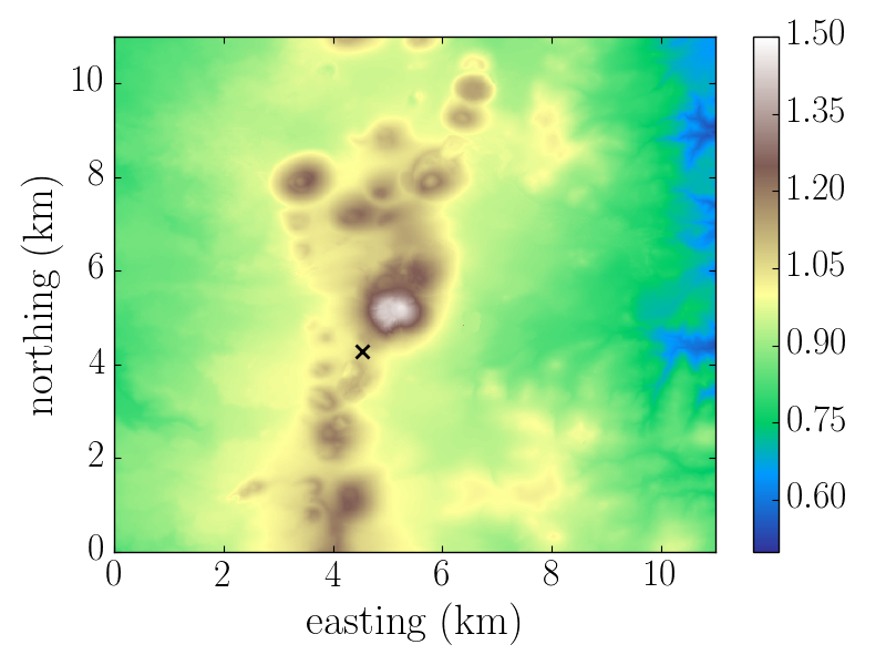
(a)

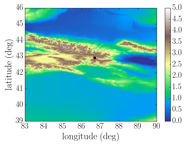
(b)

Figure 1: Elevation maps (km) of the case studies. Left: local map of the Chaîne des Puys (Lambert 93 projection). The black cross indicates the CDC location. Right: Tian Shan mountains. The black dot in the middle of the map indicates the location of the Ulastai valley.

5 Balancing speed and accuracy

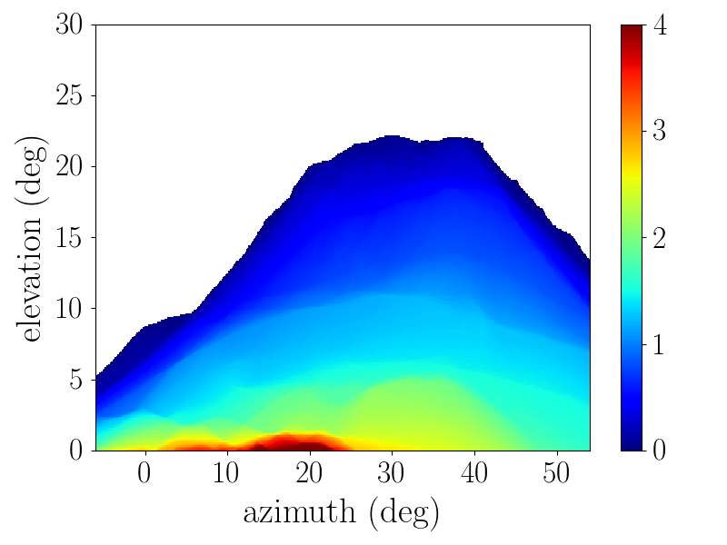
(a)

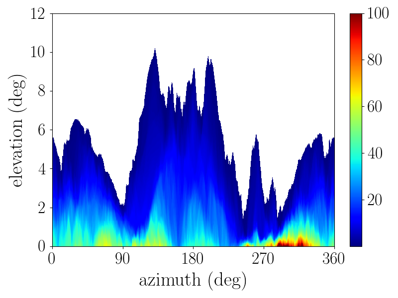
(b)

Figure 2: Rock depth (km) as function of the direction of observation. The rock depth was computed with the reference method. Left: CDC view. Right: Ulastai view. An azimuth of $0\,^{\mathrm{o}}$ points to the geographic north and an azimuth of $90\,^{\mathrm{o}}$ points to the east.

The optimistic algorithm has three tuning parameters: the slope factor, $\alpha$, the resolution factor, $s_{\mathrm{min}}$ and the binary search accuracy, $\epsilon$. In addition, TURTLE introduces a linear approximation, adding a fourth tuning parameter: the LLA range, $r_{\mathrm{LLA}}$. These four parameters allow to balance accuracy versus speed when computing the rock depth along a line of sight.

The accuracy of the binary search, $\epsilon$, can be set to rather small values without any significant increase in computation time. This can be understood since most steps do not cross a boundary, i.e. do not trigger a binary search. Furthermore, the convergence speed of the binary search goes as $1/\ln(\epsilon)$. In TURTLE, $\epsilon$ is set to a constant value of $10^{-8}\,$m which is well below the typical accuracy of DEMs.

Estimating the accuracy of the computation is not as straightforward as it might first seem. Systematically setting small step lengths results in the accumulation of numerical rounding errors on large distances. For example, incrementing the position by steps of 1 cm results in a few mm deflection after 100 km, using a 8 bytes double. In the Ulastai view, this leads to errors of several meters on the rock depth for some peculiar trajectories that are grazing the ground. In the particular case of a straight line trajectory, this can be solved by computing the step positions, $\vec{r}(s)$, from the line parametric equation instead of incrementing them by 1 cm, i.e. as:

$$\vec{r}(s)=\vec{r}_{i}+s\frac{\vec{r}_{f}-\vec{r}_{i}}{|\vec{r}_{f}-\vec{r}_{i}|}$$ (6)

with $s$ the curvilinear abscissa (distance) of the step and $\vec{r}_{i}$ ($\vec{r}_{f}$) the initial (final) position. However, in the general case this is not possible since the particle direction changes at each step.

For the present study, a reference set of rock depths is computed with a slope factor of $\alpha=1\,\%$ and a resolution factor of $s_{\mathrm{min}}=1\,\mu\mathrm{m}$. No local approximation is used and the step position is computed from equation 6. This reference set is cross-checked against rock depths obtained with a constant initial step length of $s_{0}=1\,$cm and positions computed from equation 6 as well. Note that the latter computation requires 20 CPU-days in the case of the full Ulastai view, with 217,921 lines of sight. Therefore, we do not use a step length lower than 1 cm. The reference case almost always produces identical results than the $1\,$cm case, while being $\times$100 faster. In the few cases where differences are observed, decreasing the initial step length to $s_{0}=1\,\mathrm{mm}$ for these specific trajectories shows that the reference case is correct instead of the $s_{0}=1\,$cm computation. The rock depths computed with the reference case are shown in fig. 2. The typical value in the Chaîne des Puys area is a few km. In contrast, in the Ulastai valley, the visible rock depth can be above 100 km, close to the horizontal.

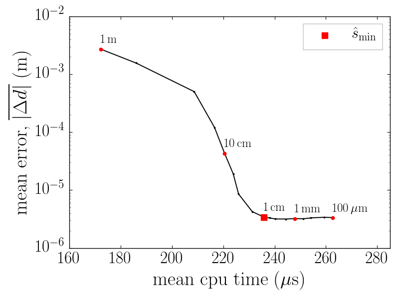
(a)

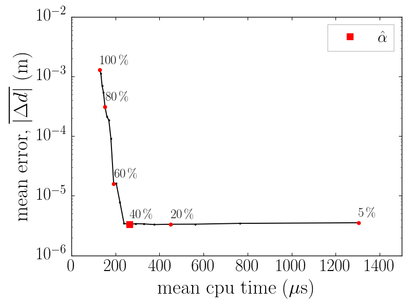
(b)

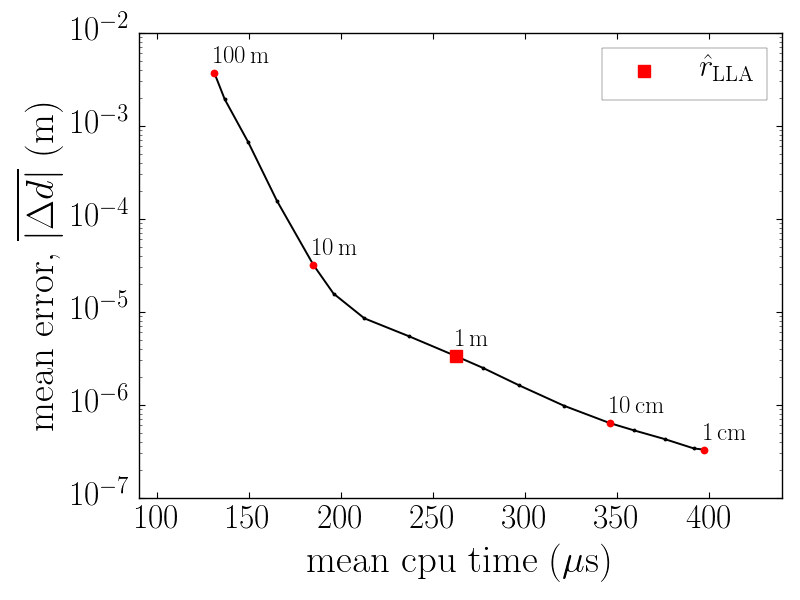
(c)

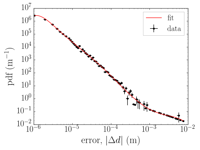
(d)

Figure 3: Accuracy versus CPU time for the CDC view when moving the tuning parameters away from the selected values ($\alpha=40\,\%$, $s_{\mathrm{min}}=1\,\mathrm{cm}$, $r_{\mathrm{LLA}}=1\,\mathrm{m}$) indicated by a red square. Top left: variation with the resolution factor. Top right: variation with the slope factor. Bottom left: variation with the LLA range. Bottom right: error distribution for the selected parameter values. The red line shows the result of a 7^th order polynomial fit in log coordinates.

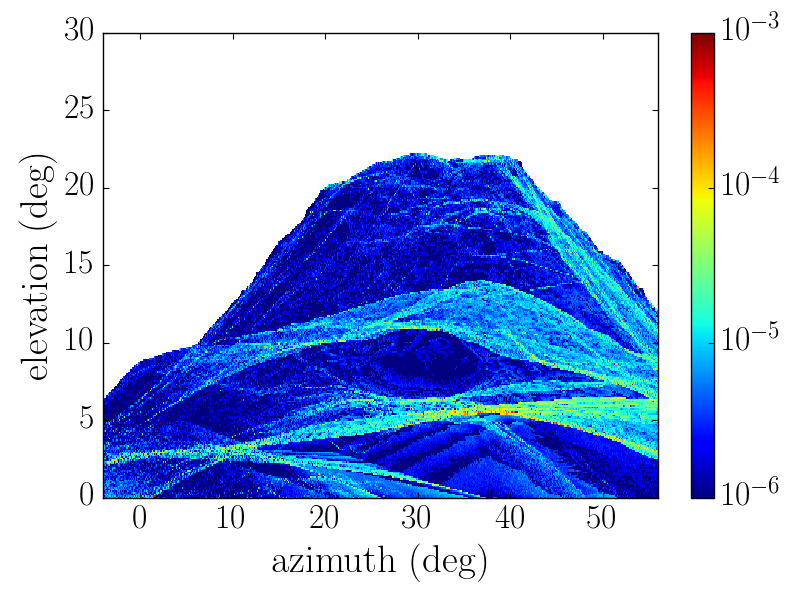
(a)

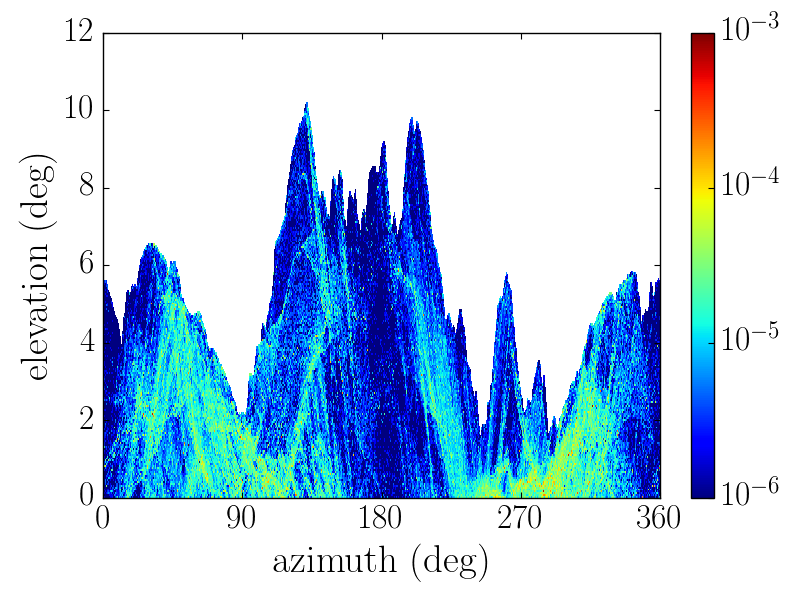
(b)

Figure 4: Error on the rock depth (m) as function of the direction of observation. The rock depth was computed with the optimistic algorithm using the selected parameter values: $\alpha=0.4$, $s_{\mathrm{min}}=1\,\mathrm{cm}$ and $r_{\mathrm{LLA}}=1\,\mathrm{m}$. Left: CDC view. Right: Ulastai view.

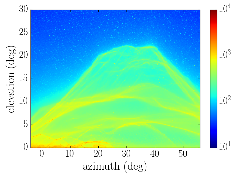
(a)

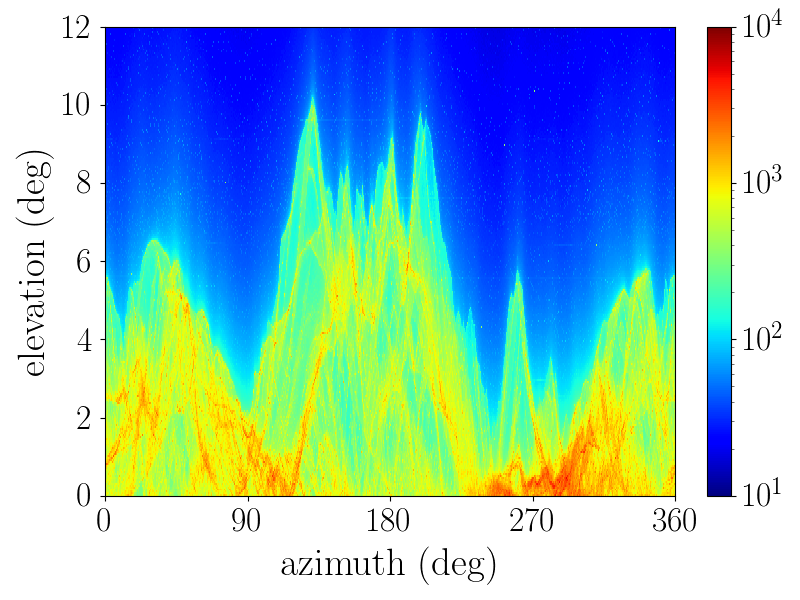
(b)

Figure 5: CPU time ($\mu$s) for computing the rock depth as function of the direction of observation. The rock depth was computed with the optimistic algorithm using the selected parameter values: $\alpha=0.4$, $s_{\mathrm{min}}=1\,\mathrm{cm}$ and $r_{\mathrm{LLA}}=1\,\mathrm{m}$. Left: CDC view. Right: Ulastai view.

We scrutinize the parameters of the stepping algorithm. The rock depth for the two views are computed for various parameter values using the turtle_stepper_step function. The track position is incremented step by step as it would be in a MC. The absolute value of the difference, $|\Delta d|$, w.r.t. the reference result is taken as an estimate of the overrunning error on the rock depth, $d$. As a figure of merit we consider how the mean error varies as function of the mean CPU time, averaging over all lines of sight of a same view. Using this figure of merit, the following set of parameters has been selected: $\alpha=40\,\%$, $s_{\mathrm{min}}=1\,\mathrm{cm}$ and $r_{\mathrm{LLA}}=1\,\mathrm{m}$, since it yields a good compromise between speed and accuracy for the two views. Figure 3 shows how the performances evolve when modifying the tuning parameters, one by one, around the selected values. Figure 3 corresponds to the CDC view, but similar results are obtained for Ulastai one. The selected parameters are located close to a break point. Reducing them below the selected value results in large CPU increase for little accuracy gain. For the selected parameter values, it is also cross-checked that computing the steps positions from equation 6, rather than incrementing them, does not significantly reduce the error.

Figure 4 shows the error on the rock depth, $|\Delta d|$, for the selected parameter values. The mean of the error on the rock depth is low, 7 to 9 $\mu$m depending on the view. The sign of the error is positive in $50\,\%$ of the cases, i.e. there is an even probability to over or under estimate the distance. This is a strong result, since it shows that the optimistic algorithm, though error prone, is not biased. The magnitude of the discrepancy is only loosely correlated to the total rock depth: 5 % correlation factor for the CDC view and 0.5 % for the Ulastai one. For the two views that we consider, with the selected parameters, all errors are below $1\,$cm except for one line of sight in the Ulastai view. For an observation angle of (55.4 ^o N, 1.35 ^o U) an error of 1.4 m occurs. Though, the relative error is of $49$ ppm only. This problem is due to a very sharp peak, located at ($43.093675\,^{\mathrm{o}}$ N, $87.038318\,^{\mathrm{o}}$ E), for which the last meter before the summit is cut through. Reducing the slope parameter to $\alpha=0.2$ allows to resolve the top of this peak for horizontal trajectories, but this comes at the cost of a 81 % CPU increase.

A detailed look at individual tracks shows that the tail events, with errors of several mm, are due to trajectories grazing the topography, i.e. being almost parallel to some parts of the ground. These effects are visible on the error maps of Puy de Dôme (top plots of fig. 4). In particular, on the left plot (CDC view) one clearly sees details of the Puy de Dôme surface due to grazing rays. The top area of Puy de Dôme (above 10$\,{}^{\mathrm{o}}$) is very steep from this side. The lines of sight make a large angle with the slope of the volcano, and a good resolution is achieved. However, In the bottom area the slope is milder. As a result the lines of sight graze the ground smoothing out its roughness and leading to a poorer accuracy. It also explains the larger correlation observed between $|\Delta d|$ and the total rock depth. The Ulastai view is more complex since a single line of sight can include several features: summits, valleys, etc. The absence of correlation between $|\Delta d|$ and the total rock depth confirms that errors result from local peculiarities, e.g. a line of sight grazing a plateau, rather than from an accumulation of numerical errors.

The consumed CPU time for each line of sight is shown in fig. 5. Depending on the direction of observation, the CPU time varies by 2 to 3 orders of magnitude from 10 $\mu$s to 10 ms. The CPU time increases abruptly when crossing rocks. The lines of sight crossing rocks, half of the total number, amount to 90 % of the CPU of a view. The CPU time is mainly driven by the rock depth, with correlation factors of 73 % (Ulastai), and 87 % (CDC). The secondary factor is the number of boundaries to map, i.e. the complexity of the topography. In addition, close to the horizontal, the CPU cost also increases due to the very long paths needed in order to reach the exit altitude, e.g. $\sim$110 km at $0\,^{\mathrm{o}}$ of elevation in order to reach 2 000 m high, starting from Col de Ceyssat. The consumed CPU time is approximatively proportional to the number of Monte Carlo steps used in order to map a line of sight. The average ratio is of 0.5 $\mu$s per step for the CDC view.

6 Comparison with ray tracing algorithms

We compare the optimistic algorithm discussed herein with the two alternative ray tracing algorithms discussed in the introduction: a BVH tree and a polyhedral mesh. In both cases the topography surface is modelled with triangular facets, joining the data nodes, and using ECEF coordinates. The data nodes of a same grid are regularly spaced in geodetic or projected coordinates. Then, a square cell defined by four adjacent nodes is split in two triangular facets, dividing the bottom right and the top left of the cell, as illustrated on the left side of fig. 6. For the polyhedral mesh, the geometry is divided in 3D cells using triangular prisms. For each triangle of the tessellated topography surface we define a top (bottom) triangular prism, having the triangular facet as bottom (top). The sides of the prisms are all parallel, defined by the local vertical at the middle of the topography. The right side of fig. 6 shows a schematic of the top and bottom prisms of a triangular facet.

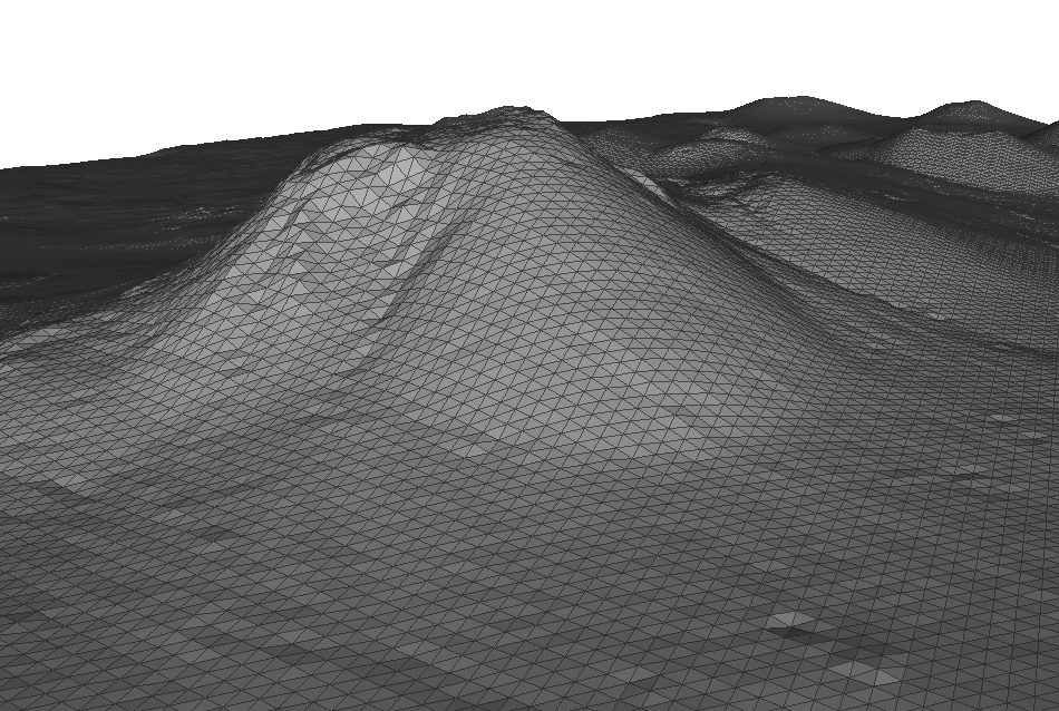
(a)

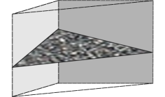
(b)

Figure 6: Tessellation of the topography data for the BVH and polyhedral mesh algorithms. Left: tessellation of the ground surface using triangular facets joining the nodes. Right: schematic of a prism cell used for the tetrahedral mesh. The original triangular facet is the textured one.

Tessellating a topography surface with triangles is a classical representation of a terrain. Let us recall that it differs from our approach which performs a bilinear interpolation of the terrain between nodes. As an example fig. 7 shows a vertical slice of the Chaîne des Puys topography modelled with the two methods. On a large scale no difference is visible (fig. 7, left). However, when zooming down to the grid resolution, discrepancies of several cm can be observed on the location of the ground between two grid nodes (fig. 7, right). For grazing rays, this can result in differences on the rock depth of the order of the spacing between grid nodes, i.e. several meters in this case.

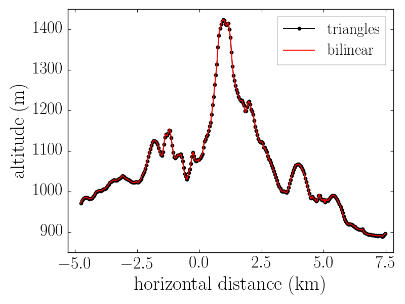
(a)

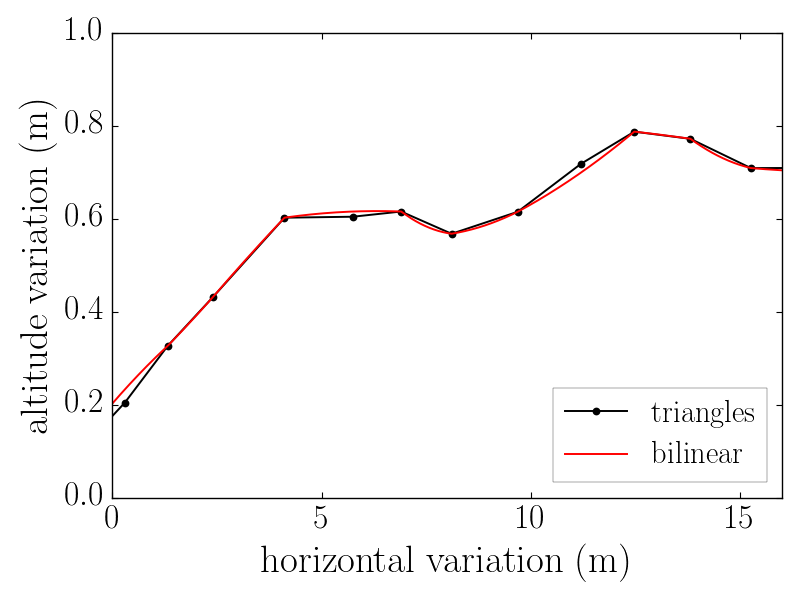
(b)

Figure 7: Vertical section of the inner topography data at an azimuth of 26^o from the CDC site. Red: bilinear interpolation (TURTLE). Black: triangular facets (BVH and polyhedral mesh). The dots indicate the intersection points with the borders of individuals facets. Left: full section but showing only one out of 30 facets intersections. Right: zoom at a horizontal distance of 880 m south of the CDC site.

Both competitor algorithms are implemented using the CGAL library [27] (v4.13), with a CGAL::Simple_cartesian<double> Kernel, as well as the ECEF conversion and geographic projection routines from the TURTLE library. Note that for the BVH method other libraries have been investigated as well, see e.g. Embree [28] in A. The CGAL library was chosen because it yields a good balance between speed and accuracy for ray tracing problems. For the BVH method we use the generic AABB tree algorithm of Alliez et al. [29] with CGAL::Triangle_3 primitives. The full geometry and its bounding boxes needs to be instantiated resulting in a high memory overhead: 350 bytes per grid node. Once initialised, the all_intersections method of the CGAL::AABB_tree provide a fast computation of all intersections of the topography surface with a ray. However, the intersections with the CGAL AABB tree are not ordered w.r.t. the ray origin. Therefore getting the closest intersection actually requires checking all intersections. Note that while the CGAL::AABB_tree has a first_intersection method, it was found to be significantly slower ($\sim$2$\times$) than looping over the result of all_intersections in order to find the closest one.

For the polyhedral mesh, a CGAL::Plane_3 object is used in order to represent the prisms facets, positively oriented towards the outside of a cell. The CGALL::Plane_3::has_on_positive_side method allows to test if a point lies on the inner or outer side of a facet. Since a triangular prism is a convex volume, a point is located inside if and only if it is on the inner side of all of its facets. Using triangular prisms instead of tetrahedra allows to reduce the total number of facets to test when navigating through the geometry. The total memory usage is kept low by creating and destroying the prisms on the fly from the raw topography data.

The rock depth along a line of sight is computed following pseudocode 1. In the case of the BVH algorithm the volume_at function is implemented by counting the number of intersections of a vertical ray with the topography surface. An even number of crossings implies that the initial position is below the tessellated ground. Then, the distance_to function proceeds by locating the closest intersection with a ray along the line of sight. The intersection points define segments. The rock depth is computed from the length of the segments lying below the surface. Note that in this particular case where trajectories are straight, it is more efficient to map all intersections with the BVH in a single step, since the CGAL algorithm provides all of them by default. For the purpose of this comparison, both methods are implemented for the BVH, i.e. getting all intersections in a single row, or stepping from one to another as in a MC.

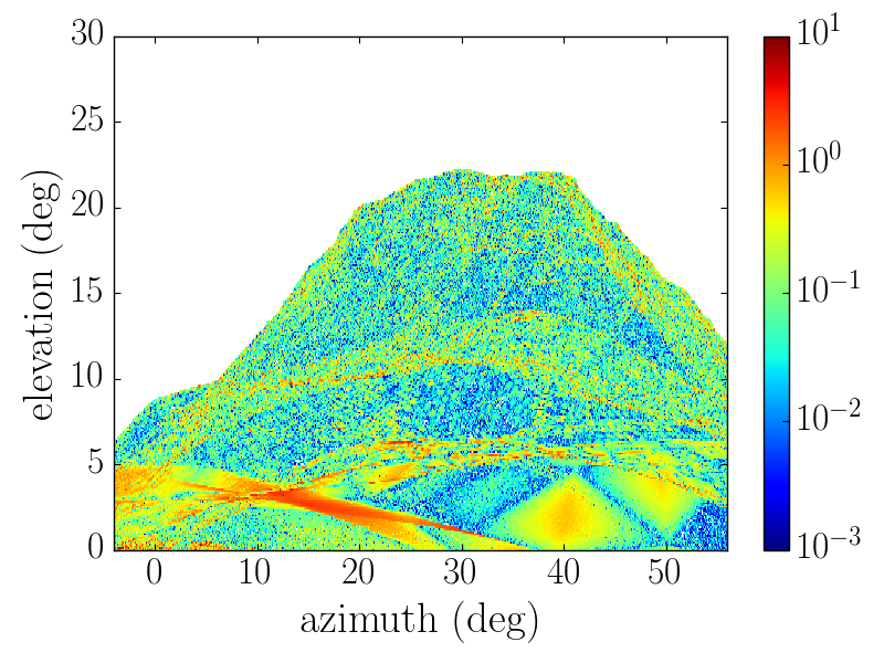
(a)

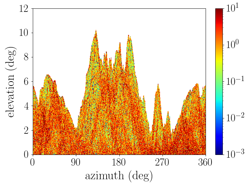
(b)

Figure 8: Absolute differences on the rock depth (m), $|\Delta d|$, as function of the direction of observation, when interpolating the DEM with triangular facets or with a bilinear model. Left: CDC view, right: Ulastai view.

For the polyhedral mesh, the volume_at function proceeds in two steps. First we locate the closest grid node using geodetic or projected coordinates. Then we test the prisms connected to this node. Once the initial volume is located, we step through the prisms and locate the intersections with the top or bottom facets. Note that since the prisms are connected by their facets their is no need to re-locate the next prism when exiting the current one. The exit facet determines the next sub-volume.

Fig. 8 shows the absolute difference on the computed rock depth, $|\Delta d|$, when using triangular facets or a bilinear interpolation of the DEM data. A striking feature is that theses differences are much larger than the overrunning errors of the tuned optimistic algorithm (fig. 4). For the CDC view the average absolute difference on the distance is 12 cm. For the Ulastai view the average value is ten times higher: 118 cm. The fact that the differences are ten times larger for the Ulastai view is consistent with the ten times larger grid spacing for the SRTMGL1 data than in the inner grid used for the Chaîne des Puys. It was also checked that the signed differences, $\Delta d$, are evenly distributed in all three cases with an average consistent with zero. The distribution of the absolute difference on the rock depth, $|\Delta d|$, is shown on the right of fig. 9. For comparison, the distribution of the absolute height difference $|\Delta z|$, is also shown on the left of the same figure 9. On average, those are approximatively five times smaller than the differences on the distance: $\langle|\Delta z|\rangle=2\,$cm for the CDC view and $19\,$cm for the Ulastai one.

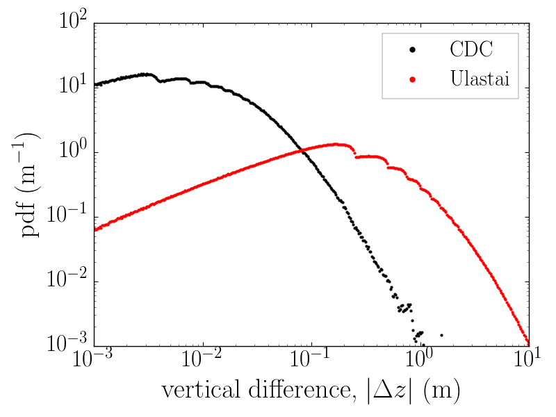
(a)

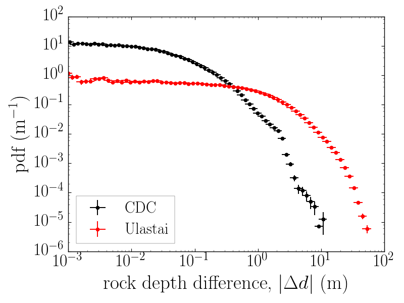
(b)

Figure 9: Statistics of the modelling differences when using triangular facets or a bilinear interpolation. Left: distribution of the absolute height difference, $|\Delta z|$. Right: distribution of the absolute difference on the rock depth, $|\Delta d|$.

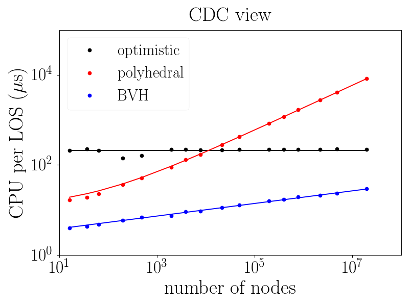
(a)

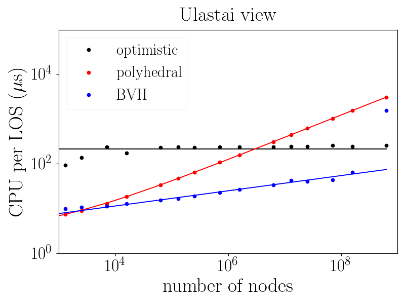
(b)

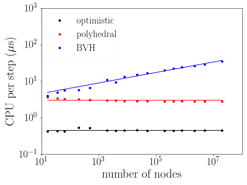
(c)

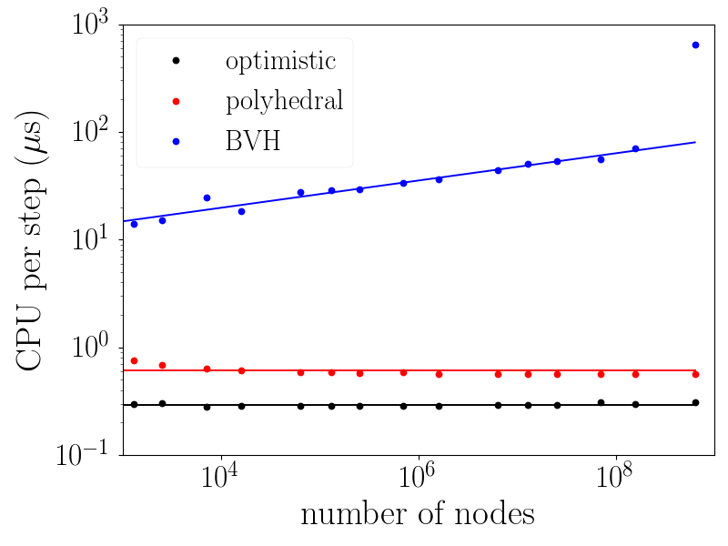
(d)

Figure 10: CPU time ($\mu$s) as function of the number of grid nodes. Black: optimistic algorithm. Red: polyhedral mesh. Blue: BVH tree. The solid lines correspond to the fit models described in the text. Upper: average CPU per line of sight for the CDC (left) and Ulastai (right) views. Bottom: CPU per Monte Carlo iteration for the CDC (left) and Ulastai (right) views.

The performances of the three algorithms are compared by varying the number of nodes of the DEM data. A periodic down sampling is applied in order to vary the number of nodes. We record the CPU time and the number of Monte Carlo steps for each line of sight. The upper part of fig. 10 shows the average CPU time per line of sight as function of the number of nodes. Numeric values are also reported in table 2 for the case when no down sampling is applied. For the BVH algorithm intersections are computed in a single row. Clearly, the BVH algorithm performs the best when it only comes to map all intersections of the topography with a straight ray. The CPU time only slightly increases with the number of nodes. The increase rate is found to follow a power law: $an^{b}$, with an exponent of $b=1/8$. However, for the full Ulastai data 200 GB of RAM are needed out of which the initial elevation data represent only 1.2 GB. As a result the test server needs to use its swap memory, resulting in a slowdown by a factor of ten when no down sampling is applied. Furthermore, when the geometry has more than $n=10^{7}$ nodes, the initialisation of the BVH requires more time than scanning all the $\sim$200,000 lines of sight. The polyhedral mesh algorithm is not efficient for intersecting large grids. Its CPU time is fitted with a square root law: $a+b\sqrt{n}$, in agreement with expectations. Interestingly, the performances of the optimistic algorithm do not depend on the number of nodes, but only on the ray length and the topography features. As a result it outperforms the polyhedral mesh for grids larger than $1000\times 1000$ nodes. In principle it should also be faster than the BVH algorithm for extreme grid sizes. But, the large amount of memory required by the BVH is likely to be an issue before this happens. Let us recall that in contrast to a BVH, TURTLE’s implementation of the optimistic algorithm requires no more memory than the initial elevation data.

In the case where the step sizes are limited by the physics, the relevant parameter is the average CPU time spent at each MC step in order to resolve the geometry. An estimate of this quantity is provided by the total CPU time for all lines of sight of a view divided by the total number of transport steps. In the case of the BVH algorithm it is relevant to consider the CPU time with stepping in this case. The CPU time per MC step is indicated on the lower part of fig. 10 and in column four of table 2. In this configuration the BVH algorithm is inefficient. The optimistic algorithm performs best. It is a hundred times faster than the BVH algorithm, for large grids. The polyhedral mesh is two (six) times slower than the optimistic algorithm, for the Ulastai (CDC) view. However, the present comparison of the polyhedral versus optimistic algorithm should be considered with precaution. The CPU time per step can vary strongly in both cases, depending on the step length dictated by the physics. In the polyhedral case, the first step in a prism is much longer than the subsequent one, since the local geometry needs to be built. A closer analysis, using valgrind [30] & callgrind [31], shows that building the prisms on the fly represents 75% (Ulastai) to 93% (CDC) of the CPU instructions of a Monte Carlo step, with our implementation. In the present study each prism is traversed in a single step, which is the worst case. Similarly, for the optimistic algorithm, depending on the set LLA range, successive small steps are accelerated by TURTLE.

View	Algorithm	Steps	CPU ($\mu$s)
		per LOS	per LOS	per step
CDC	BVH	2.8	22 (51)	18
	Optimistic	497	261	0.52
	Polyhedral	2 975	8 353	2.8
Ulastai	BVH	4.3	46∗ (213∗)	49∗
	Optimistic	840	293	0.35
	Polyhedral	5 492	3 233	0.59

Table 2: Comparison of the performances of the BVH, optimistic and polyhedral ray tracing algorithms for the 2 view points (CDC & Ulastai) without down sampling. The CPU times are averages per line of sight or per transport step. The average number of transport steps per line of sight are reported as well. For the BVH algorithm the CPU time with and without stepping are quoted. $(^{*})$ For the Ulastai view with the BVH algorithm, due to memory issues, the quoted CPU times are actually extrapolations from a down sampled topography using the power law model described in the text.

Looking back at fig. 10, or table 2, one might wonder why for the polyhedral mesh, the CPU time is five times larger in the CDC view than in the Ulastai one. A detailed analysis with callgrind shows that this is due to the fact that the Chaîne des Puys inner map uses Lambert 93 projected coordinates, whose conversion has a high CPU cost: six times more instructions than when using geodetic coordinates. As a result, building the prism geometry is very inefficient. This could be solved by re-meshing the elevation data in geodetic coordinates, or even better, directly in a plane projection in ECEF coordinates. The optimistic algorithm uses a TURTLE stepper with a 1 m LLA range. It mitigates the CPU overhead introduced by the map projection. As a result, the CPU time is only two times larger in the CDC view than in the Ulastai one.

7 Performances in Monte Carlo simulations

When integrated in a MC, the ray tracing methods introduce a slowdown w.r.t. the pure physics processing. This slowdown arises from two factors. First, computing the geometric step length adds an extra CPU cost at each Monte Carlo step. This factor is common to all geometry navigation methods. The optimistic and polyhedral mesh methods are designed in order to minimise this cost. However, they add a second slowdown factor by increasing the total number of Monte Carlo steps required for the navigation through the geometry. Depending on the CPU cost of each step, and the number of added steps, limiting the geometric step length might be worth or not.

In order to check the performances of the TURTLE library, when integrated in a MC, let us consider a classical problem for muography applications: the computation of the atmospheric $\mu$ flux for each line of sight of the two views previously considered. Such a problem is efficiently solved using a reverse Monte Carlo method, where the particles are tracked backward from the detector to the source. Note that even though the Monte Carlo flow is reversed, the time flow is not. Reverse Monte Carlo is a particular MC sampling method. It does nor revert time neither solve an inverse problem. In the following we use the words initial and final w.r.t. time, i.e. in their usual meaning. The PUMAS [22] library provides a reverse Monte Carlo engine for $\mu$ or $\tau$ implementing the backward method. Details of the backward method can be found in Niess et al. [32]. For the present study, version 0.14 of PUMAS is used, together with a turtle_stepper. PUMAS does not provide geometric primitives and ray tracing as for example Geant4 does. Instead the PUMAS transport engine operates on a generic geometry that must be supplied by the user as a pumas_medium_cb callback. This callback must answer to volume_at and distance_to queries. This allows to easily interface arbitrary ray tracers with PUMAS. An example of ray tracer integration can be found in the source code of the test suite [20] (function medium in file src/simulator.c). Note that in order to avoid running superfluous ray tracings, the result of the last distance_to query is cached.

The TURTLE library and its optimistic stepping scheme can also be integrated in a generic Monte Carlo like Geant4, without modifying the base engine. This is further discussed in B. However, for the present study we decided to use a less complex Monte Carlo engine, dedicated to $\mu$ transport: PUMAS.

For each line of sight, the $\mu$ spectrum is estimated by backward sampling 100 $\mu$. The $\mu$ final kinetic energy is randomised over a $1/E$ distribution between 1 MeV and 1 PeV. Note that a priori any distribution could be used for the final kinetic energy, as long as it covers the full range of possible values. Using a $1/E$ distribution is a good pick for this problem, reducing the Monte Carlo variance. It amounts to drawing the logarithm of the final kinetic energy from a uniform distribution. The particle is then positioned at the view point, oriented backwards along the line of sight. From there on it is backward transported until it reaches the primary source. The primary source is set at an altitude of 2 000 m (CDC) or 7 500 m (Ulastai), as for the ray tracing problems. The maximum kinetic energy of the primary $\mu$ source is set to 100 PeV. Above this energy the atmospheric $\mu$ flux is too low, for muography applications. Whenever a backward propagated $\mu$ exceeds this energy the tracking is stopped and its Monte Carlo weight is set to zero.

The PUMAS Monte Carlo engine can be run with different levels of detail for the physics configurable on the fly, e.g. during the tracking of a particle. For the present study we perform a detailed simulation of physical processes. The level of accuracy is comparable to Geant4 at low energy, below $\sim$1 TeV, and to dedicated high energy $\mu$ transport engines, e.g. MUM [33], above.

In a detailed simulation, due to scattering, particles observed along a given line of sight from the view point actually follow different trajectories, traversing different amounts of matter. This complicates performance studies. Therefore, the PUMAS library is modified by overriding transverse deflections to zero, such that all particles actually follow a straight trajectory along the line of sight. Note that this modification is applied after computing any deflection angle, in order to properly count the corresponding CPU cost.

The CPU cost of the physics simulation is estimated as following. Since all particles follow the same straight trajectory, for a given line of sight, the geometry can be pre-computed once for all, before actually running the MC simulation. This is done with TURTLE as well. The distances between the view point and the intersections of the line of sight with the topography are stored in a 1-dimensional table. Then, during the MC simulation the distance of the particle to the next boundary can be inferred from the table and its distance from the view point. This can be done very efficiently such that the corresponding CPU cost is negligible w.r.t. the physics simulation. Running PUMAS with this pre-computed geometry provides an estimate of the CPU cost of the physics simulation.

The CPU cost for the physics simulation depends on the $\mu$ final energy. The lower the $\mu$ energy the shorter the physical steps and the higher the corresponding CPU cost. The CPU cost also increases in rocks since the physical step length decreases by 3 orders of magnitude due to the differences in target density. This is counterbalanced by the fact that the $\mu$ path length in air, up to the primary altitude, is larger than in rocks. Averaging over all lines of sight and $\mu$ energies, the CPU cost is dominated by particles traversing rocks and reaching the view point with low energy.

Table 3 shows a summary of the mean performances per line of sight and per Monte Carlo event for the two view points. Considering the physics only, i.e. when the geometry has been precomputed, on average $\sim\,312$ (380) Monte Carlo steps are needed per line of sight for the CDC (Ulastai) view. Most of these MC steps concern the simulation of Coulomb multiple scattering. If this process is disabled only a dozen MC steps are needed for the physics simulation. In comparison, a pure ray tracing e.g. with a BVH requires only 3 (4) steps for the CDC (Ulastai) view (see table 2 in section 6). This clearly shows that for the application considered here most Monte Carlo steps are limited by physics processes.

When the optimistic ray tracing is integrated in the MC simulation, the average number of steps doubles for both views. One might notice that for the Ulastai view the number of Monte Carlo steps with ray tracing (797) is actually lower than what was found previously (840) in section 6. This is due to the fact that the backtracking is stopped when a $\mu$ energy exceeds $100\,$PeV, which corresponds approximatively to the traversing of $\gtrsim 10\,$km of rocks. This seldom occurs in the CDC view where the largest rock depth crossed is of $5.0\,$km. On the contrary, for the Ulastai view the largest rock depth is of $117\,$km with an average value per line of sight of $6.7\,$km.

Figure 11 shows the slowdown induced by the optimistic ray tracing, defined as the ratio of the CPU cost with ray tracing to the one of the physics, i.e. with a pre-computed geometry. Similar results are obtained for both views. On average, the optimistic ray tracing doubles the CPU cost w.r.t. the physics simulation. However, locally higher slowdowns (5-6) can be observed for grazing rays. In such cases the number of Monte Carlo steps increases by one order of magnitude. The average performances of the optimistic algorithm are very good given the large number of topography nodes considered here. The cost of the geometry resolution is kept at the level of the physics simulation. It implies that whatever the efficiency of a ray tracer algorithm, at best it could speed up the present Monte Carlo simulation by a factor of two.

View	Steps		CPU (ms)
	Pre-comp.	Optimistic	Pre-comp.	Optimistic
CDC	312	695	0.9	2.2
Ulastai	380	797	1.0	2.2

Table 3: Comparison of the Monte Carlo performances using the optimistic (TURTLE) ray tracing or a pre-computed geometry for the navigation. The results are given for the two view points (CDC & Ulastai) without any down sampling. The quoted CPU time and number of Monte Carlo steps are averages per line of sight and per Monte Carlo event.

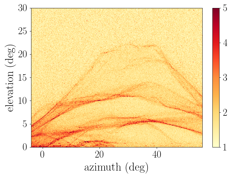
(a)

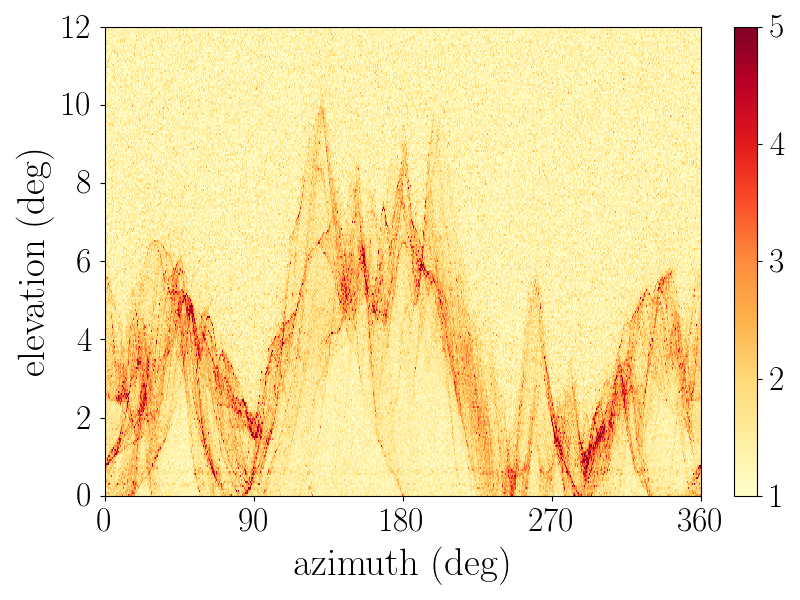
(b)

Figure 11: Monte Carlo slowdown factor as function of the direction of observation when computing a $\mu$ spectrum with PUMAS. The slowdown is defined as the ratio of the Monte Carlo CPU with ray tracing to the one of the bare physics simulation. Left: CDC view, right: Ulastai view.

The Monte Carlo performances of the optimistic ray tracer have been compared with the ones achieved when using the BVH and polyhedral mesh discussed previously in section 6. Let us recall that the CGAL library [27, 29] is used for the BVH and polyhedral mesh implementations. The exact same Monte Carlo transport algorithm is used for all ray tracers. Only the volume_at and distance_to callbacks differ. The obtained numerical results are summarised in table 4. It can be seen that in this scenario where the stepping is driven by the physics, the optimistic algorithm (TURTLE) performs the best. It outperforms CGAL’s BVH even for the CDC view where the topography grid is of moderate size ( $\sim$$10^{7}$ nodes). For the Ulastai view the quoted numbers for the BVH algorithm are underestimates. Due to memory issues, the DEM was down-sampled by a factor of two along both grid dimensions. Otherwise, the required memory exceeds $200\,$GB resulting in a slowdown by a factor of 10 due to swapping between the RAM and the hard drive. Note that the CGAL BVH algorithm is particularly inefficient in this situation because it maps all intersections with the topography at each ray tracing query, instead of just the closest one. More efficient BVH exist in this situation, as shown in A. An optimised BVH ray tracer might improve the Monte Carlo CPU performances over TURTLE (the optimistic algorithm), while providing a similar accuracy. However, for large DEMs this would be at a high memory cost ($\sim$$100\,$GB) for a moderate CPU gain (a factor of two at best).

The polyhedral mesh performs surprisingly well in the Monte Carlo of the Ulastai view. It is only two times slower than the optimistic algorithm. This is due to the fact that the backtracking is interrupted for long range particles, i.e. close to the horizontal, because the $\mu$ would be of too high energy as discussed previously. This is reflected as well on the number of Monte Carlo steps which is significantly lower in the Monte Carlo ($3\,331$) than for the pure ray tracing ($5\,492$, see table 2). However, for the CDC view the polyhedral mesh performs poorly because of the extra CPU cost due to the coordinates conversion from Lambert projection to ECEF, as observed in previous section 6. TURTLE mitigates this cost by using a Local Linear Approximation (LLA) which makes the comparison with the polyhedral mesh unfair in this case. Properly optimised the polyhedral mesh could be competitive with the optimistic algorithm when the stepping is driven by the physics. The polyhedral mesh is however inefficient for pure ray tracing problems over large DEMs, e.g. transporting weakly interacting particles like neutrinos. Therefore, it is less versatile than the optimistic algorithm.

View	Algorithm	Steps	CPU
		per LOS	per LOS (ms)	per step ($\mu$s)
CDC	BVH	310	8.0	26
	optimistic	695	2.2	3.2
	polyhedral	3 169	11	3.6
Ulastai	BVH	> 378∗	> 21∗	> 59∗
	optimistic	797	2.2	2.8
	polyhedral	3 331	5.0	1.5

Table 4: Comparison of the Monte Carlo performances using a BVH algorithm for the ray tracing, the optimistic algorithm (TURTLE) or a polyhedral mesh. The average CPU times per line of sight and per Monte Carlo step are reported as well as the average number of Monte Carlo steps. $(^{*})$ For the BVH of the Ulastai topography the DEM was down-sampled by a factor of two along both grid dimensions due to memory issues.

8 Conclusion

The optimistic algorithm is an efficient method for navigating through topographies. Contrary to traditional ray tracing methods, the optimistic algorithm proceeds by trials and errors. It takes the risk of overrunning some details of the geometry. In the case of a topography described by a DEM, this risk can be efficiently controlled by adapting the stepping distance as a function of the height above ground. Using this strategy, errors are kept below the native accuracy of DEM data. In addition, the optimistic algorithm naturally handles higher interpolation models between the grid nodes than the traditional flat triangular facets. Differences on the rock depth of the order of the distance between the grid nodes can be observed, when using a triangular tessellation or a bilinear interpolation.

The TURTLE C library provides utilities for navigating through a topography described by a DEM using the optimistic algorithm. The elevation data of a DEM are encapsulated in turtle_map objects. Values between nodes are rendered with a bilinear interpolation. Collections of maps, as provided by global DEMs for example, are managed with turtle_stack objects. The turtle_client object provides thread safe access to stacks of maps. TURTLE supports a few cartographic projections, including UTM. The TURTLE library also provides transforms for representing the topography data in Cartesian ECEF coordinates. The top level component of the library is the turtle_stepper object. It provides navigation functionalities.

The traversal time of the optimistic algorithm does not depend on the number of nodes of the DEM grid, contrary to other methods. It only depends on the extent of the topography, and on its details. The more a ray is grazing the ground, the longer its traversal time. In addition, the optimistic algorithm was implemented in TURTLE with zero extra memory cost, apart from the initial DEM data. Thus, this method performs particularly well for large grids, with more than $10^{9}$ nodes. In such cases, while a BVH algorithm could be ten times faster it would require hundreds of GB of extra memory. Polyhedral meshes are not competitive for large scales.

The optimistic algorithm is particularly efficient when navigating through a topography in detailed MC simulations. Applied to a muography Monte Carlo, the TURTLE library allows to render a large scale topography on the fly while only slowing down the simulation by a factor of two, w.r.t. the bare physics. This is due to the fact that the optimistic algorithm provides both fast estimates of the distance to the ground together with a fast traversal time. Fast estimates are required in order to efficiently track particles that frequently change direction. BVH like optimisations are not well tailored for such cases: large number of nodes ($>10^{7}$) but with a stepping limited by the simulation of the physics. At best only moderate CPU gains could be achieved but at the cost of a large memory usage.

The current implementation based on eq. (1) could be further refined. A simple improvement would be to vary the slope parameter, $\alpha$, depending on the map region. For example in plain regions, values of $\alpha$ larger than in mountainous areas could be used. This would however require a preliminary analysis of the map data. The algorithm discussed in this paper is already very efficient, despite being extremely simple. It has no memory overhead and requires no initialisation, apart from loading the initial DEM data.

Appendix A Comparison with Embree

The rock depth along a line of sight is computed following the pseudocode 1 and using the Embree library [28] (version 3.5.2) from Intel. This library provides a highly optimised BVH algorithm exploiting the Single Instruction Multiple Data (SIMD) capabilities of CPUs. However, note that Embree uses a fixed single precision float (32 bits). On the contrary, CGAL allows arbitrary precision using templating. A CGAL::Simple_cartesian<double> Kernel was used for this work, i.e. double precision (64 bits).

As for the CGAL based algorithm, the volume_at function is implemented by counting the number of intersections of a vertical ray with the topography surface. The distance_to function is an encapsulation of Embree’s rtcIntersect1, which directly provides the closest intersection of a ray with the scene. The RTC_SCENE_FLAG_ROBUST was set, forcing Embree to use its most accurate ray tracing algorithm at the cost of downgraded CPU performances. As for the CGAL implementation, we also implemented a straight version of the distance_to function where all intersections are mapped in a single call. With the CGAL library, using the stepping version for the ray tracing is two times slower than using the straight one. However, with Embree the stepping version is only 14 % longer than the straight one.

Figures 12 and 13 show a selection of the ray tracing performances obtained with Embree. A key issue is that Embree’s native numerical accuracy is insufficient for the physics application that we consider. The ray tracing CPU performances of Embree are however impressive, outperforming CGAL by one order of magnitude. Note that the two libraries have different scopes. CGAL is a generic toolbox for applied Mathematics whereas Embree is optimized for graphics rendering on CPUs. Using Embree, the average error on the rock depth is $4.3\$m for the CDC view and $7.9\$m for the Ulastai one. Furthermore, errors as large as kilometers can occur along some peculiar lines of sight. This clearly makes Embree not directly usable for most physics applications. Note that Embree also allows custom geometries to be used. This is done via user supplied callbacks implementing the bounding box computation and ray intersection functions. It might be possible to improve the numerical accuracy by using a custom double precision geometry with a slower but more accurate math library. Note however that Embree’s internal representation of bounding boxes would still be in single precision. Implementing and optimising this is beyond the scope of the present paper.

Despite its insufficient numerical accuracy, the Embree ray tracer was also tested in the Monte Carlo scenario of section 7, i.e. for a muography application using PUMAS. The CPU performances are excellent with an average slowdown of only 40 % w.r.t. the physics simulation. This number could be considered as a lower limit of the performances that could be achieved in such a scenario. Note however that there is a trade to play between speed an numerical accuracy such that an accurate enough implementation for physics application is likely to be slower than what is achieved with Embree’s native ray tracer.

View	Steps		CPU (ms)
	Pre-comp.	Embree	Pre-comp.	Embree
CDC	312	304	0.9	1.3
Ulastai	380	377	1.0	1.4

Table 5: Comparison of the Monte Carlo performances using the Embree ray tracer or a pre-computed geometry for the 2 view points (CDC & Ulastai) without down sampling. The reported CPU time and number of Monte Carlo steps are averages per line of sight and per Monte Carlo event.

Finally, let us point out that the CPU time required to build the BVH scales linearly with the number of grid nodes for both libraries. The BVH initialisation requires $1.3\,\mu$s per node for Embree against $2.6\,\mu$s for CGAL. The memory usage of Embree is lower as well: 185 bytes per node. This is approximatively half the requirements of CGAL which is consistent with the fact that Embree uses single precision floats whereas double precision was used with CGAL.

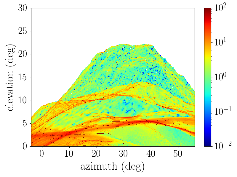
(a)

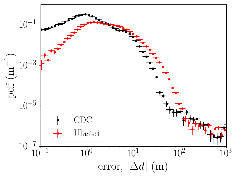
(b)

Figure 12: Absolute error on the rock depth (m), $|\Delta d|$, using Embree. Left: error for the CDC view as function of the direction of observation. Right: distribution of the error for the CDC (black) and Ulastai (red) views.

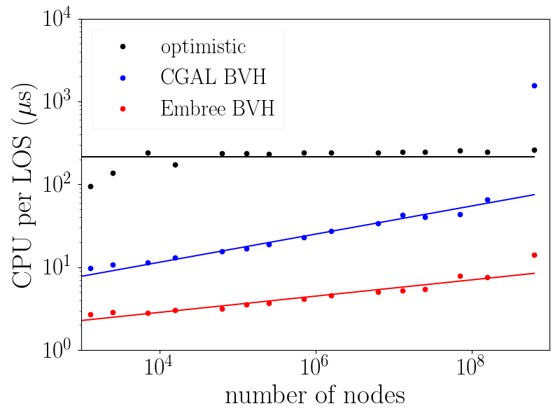
(a)

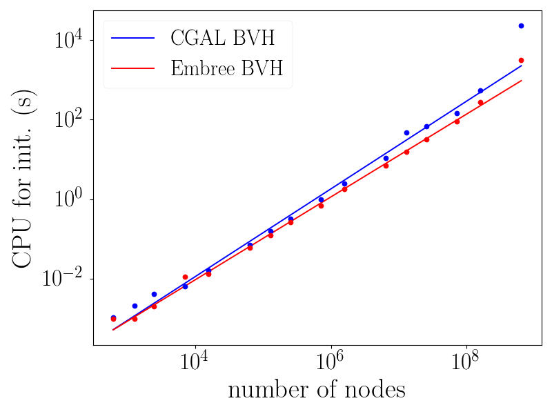
(b)

Figure 13: CPU performances for the Ulastai view as function of the number of nodes. Left: average CPU time ($\mu$s) of the ray tracing per line of sight. Right: CPU time (s) required for initialising the BVH. Black: optimistic algorithm. Red: Embree BVH. Blue: CGAL BVH.

Appendix B Application to Geant4: G4Turtle

The G4Turtle class provides an example of interfacing of the TURTLE library with Geant4. It encapsulates a turtle_stepper object and its related data : turtle_map, & turtle_stack. The source code is available from GitHub [34] under the LGPL-3.0 license. The G4Turtle interface is provided as a demonstration that the TURTLE library can be integrated in a generic Monte Carlo like Geant4, without modifying the base engine. We do not claim that the present implementation is the most optimal one. In particular, it does not support multi threading and it requires disabling the SmartVoxels navigation at the topography level. It is functional though, with a mild CPU slowdown per Monte Carlo step. Below we provide an overview of the G4Turtle class followed by validation tests and performance comparisons. The corresponding source code is available from the test suite [20].

B.1 Description of the implementation

In Geant4 a geometry is described by a set of volumes bounded by G4VSolid objects, e.g. G4Box, G4Orb, $\ldots$ and filled with G4Materials. These volumes are ordered by inclusion relations. The top volume is called World. Each G4VSolid implements in particular the Inside, DistanceToIn and DistanceToOut methods. These methods allow to check if a particle is inside or outside of the volume, and to compute the distance to the volume border, following a straight line along the particle direction. Note that for these latter methods, Geant4 expects an exact distance to be returned, given the particle direction. In order to implement the optimistic algorithm without modifying the G4Navigator, a static geometry must be mocked. In the following, we describe how this is done in G4Turtle.

A top level Envelope volume is defined. This volume is bounded by a top and bottom altitude, in ECEF coordinates. It contains two rock Chunks and two air Chunks sub volumes. These sub-volumes are artefacts used to steer the navigation. They have a variable position and extent. This required disabling geometry optimisations within the Envelope and its chunks, as SetOptimisation(false). Otherwise the SmartVoxels builder issues an overlap exception. Geant4 navigation starts by checking if a particle is inside the top volume, i.e. the envelope. At this stage we compute the particle altitude and the corresponding ground level using a turtle_stepper. If the particle is inside the Envelope, the Geant4 navigation will further check the sub-volumes. Given the particle altitude w.r.t. the ground, the rock or air chunks will return kInside or kOutside. Inside a Chunk, Geant4 requests the distance to the border. An optimistic estimate of the distance to the ground is returned, as given by pseudocode 5, i.e. refined with a binary search. When the navigation exits the chunk, it starts again checking if the particle is still inside the envelope. However, it does not check the chunk that was just exited. Therefore, two chunks of each material are needed.

The previous method needs to be slightly refined in order to handle extra volumes placed within the topography envelope, e.g. a detector. First, when Geant4 checks if the particle is inside the Envelope we loop over all extra sub-volumes, i.e. non Chunks. If the particle happens to be located in any of these sub-volumes, the rock and air chunks return kOutside, i.e. extra volumes have precedence over the topography. In addition, when computing the optimistic stepping distance from within a Chunk, we need to check the DistanceToIn to all extra sub-volumes. If any sub-volume is closer than the distance provided by eq. (1), the initial stepping distance is modified accordingly. If a binary search needs to be done, extra sub-volumes are checked again, at each iteration. Note that sub-volumes are traversed with a linear search since SmartVoxels navigation is disabled. Therefore, this implementation is not optimal if a large number of sub volumes is to be inserted inside the topography. SmartVoxels are however re-activated by default within sub-volumes, speeding up the navigation once inside one of them. So, complex sub volumes, e.g. a detailed detector, should be manually enclosed in simple bounding G4Box when placed within the topography envelope.

B.2 Validation and performances

The G4Turtle class is used with Geantinos in order to compute the rock depth for the two views described in section 4. Version 10.5.1 of Geant4 is used. The results are compared to the one obtained with the direct ray tracing of section 6 using the optimistic algorithm. Note that both computations use a turtle_stepper but wrapped differently. An average agreement of a few $\mathrm{\mu m}$ is found on the rock depth. While for almost all lines of sight the rock depth agrees better than 0.1 $\mathrm{\mu m}$, discrepancies up to 1 cm can be observed for a few grazing rays.

The number of steps required by the ray tracing is also in excellent agreement for both cases, within $0.1\,\%$. Profiling with valgrind shows that approximatively the same number of instructions are spent in the turtle_stepper. However, the rock depth computation using Geant4 (G4Turtle and Geantinos) is 4 times slower than the dedicated ray tracing. This can be understood since Geant4 is a generic Monte Carlo engine not specifically optimised for a pure ray tracing problem. In this case most of the CPU spent by Geant4 is for managing irrelevant functionalities for the ray tracing, e.g. G4Events, G4Tracks, etc.

The performances of the G4Turtle class have been compared to the one obtained when modelling the terrain with Geant4’s native G4TessellatedSolid geometry using G4TriagularFacets. Only the CDC view point was considered with various down-sampling values, as was done in section 6. The initialisation time of the G4TessellatedSolid increases as the square of the number of nodes. Let us recall that for CGAL and Embree’s BVH the scaling is linear instead. This prevents us for using the complete DEM data for the CDC view since the initialisation would require approximatively two weeks. Figure 14 shows the average CPU time per LOS and per step as function of the number of nodes. For a moderate number of nodes ($\leq 10^{4}$) the Geantino scan is much more efficient with a G4TessellatedSolid than with a G4Turtle geometry. However, above $10^{4}$ nodes the CPU time per step required by the G4TessellatedSolid starts to increase approximatively linearly with the number of nodes. As a result, the Geantino scan becomes more efficient with a G4Turtle geometry for grids with $10^{6}$ nodes or more.

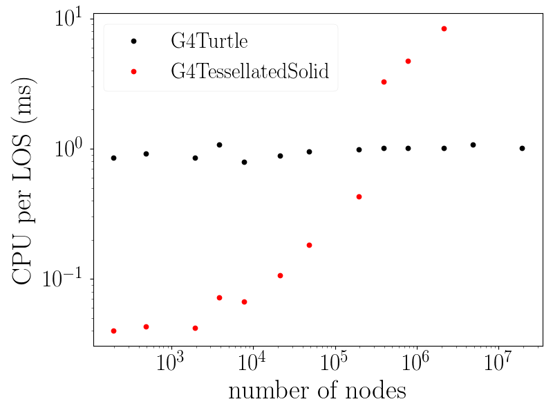
(a)

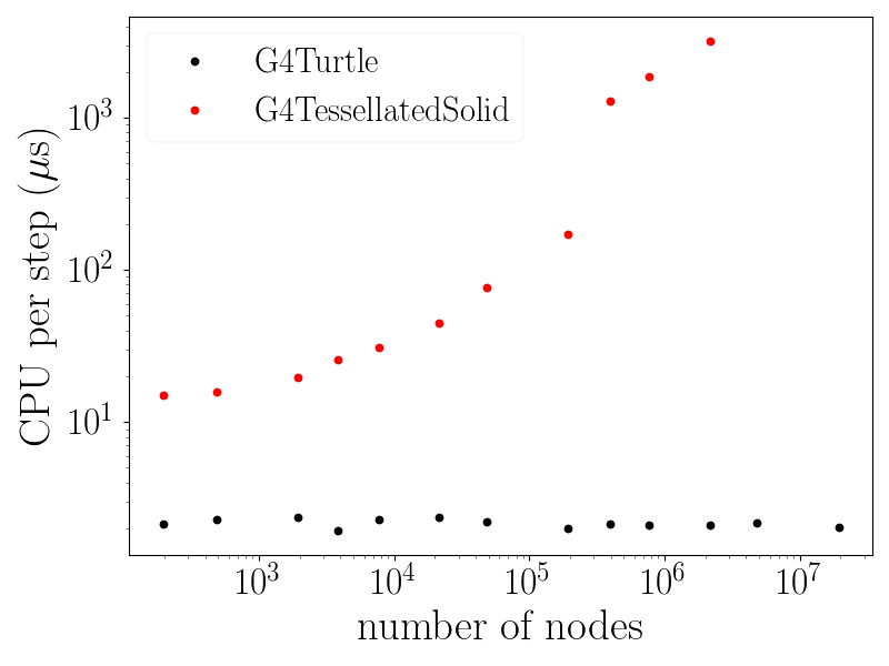
(b)

Figure 14: CPU time as function of the number of grid nodes for a Geantino scan of the rock depth seen from the CDC view point. The (black) red dots stand for the G4Turtle (G4TessellatedSolid) geometry. Left: average CPU time per line of sight. Right: average CPU time per Monte Carlo step.

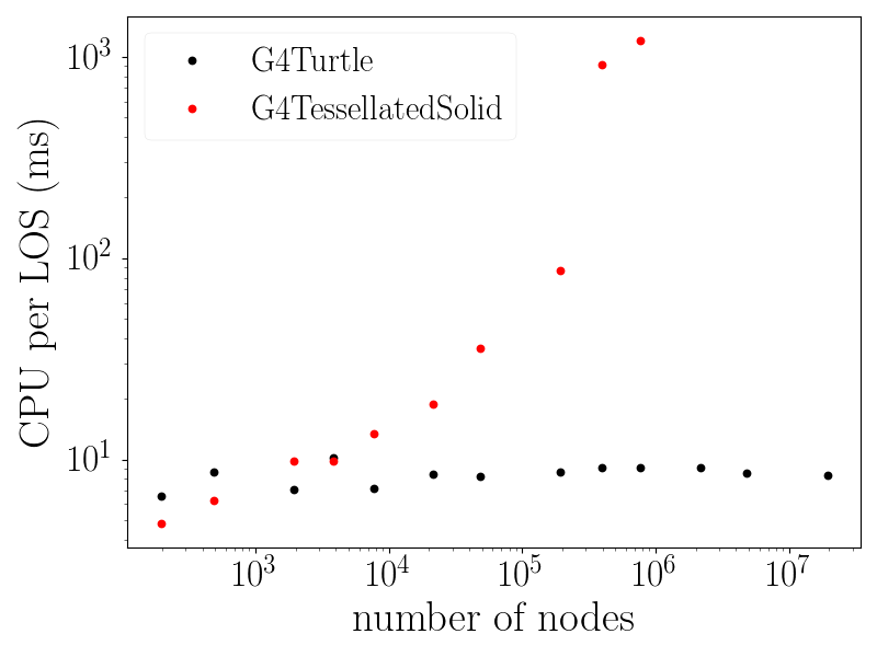
(a)

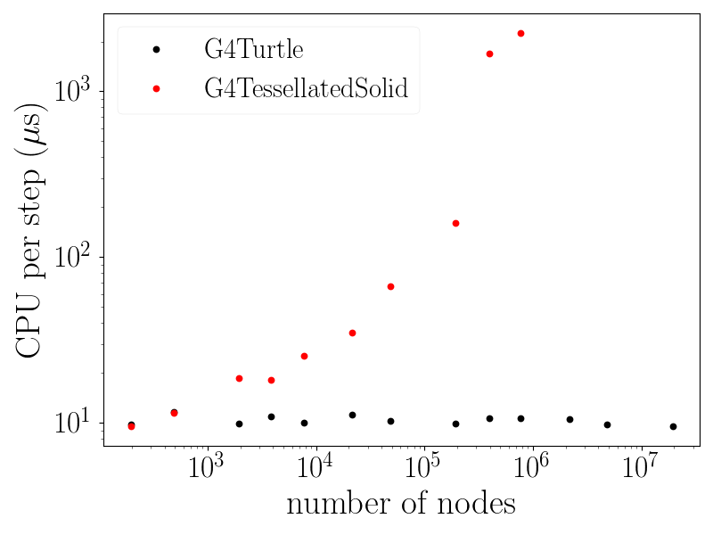
(b)

Figure 15: CPU time as function of the number of grid nodes for the transport of 10 TeV $\mu$ generated at the CDC view point. The (black) red dots stand for the G4Turtle (G4TessellatedSolid) geometry. Left: average CPU time per line of sight. Right: average CPU time per Monte Carlo step.

Let us now use Geant4 for a pure $\mu$ transport problem similar to what has been done in section 7 with PUMAS. High energy ($10\,$TeV) $\mu$ are generated at the viewpoint with an initial direction along a line of sight, pointing upward. The $\mu$ is tracked until it escapes the simulation or decays. The G4EmStandardphysics and G4EmExtraphysics modular physics list are used and secondary tracks are killed, i.e. only primary muons are tracked as with PUMAS. The total CPU cost depends strongly on the production cut value set when building the PhysicsList. For the present tests the cut value was conveniently chosen to be of $1\,$m. For muography applications this would not be accurate enough for lines of sights crossing a rock depth below $\sim$$100\,$m. However, cut values below 1 m significantly slow down the $\mu$ transport by increasing the number of Monte Carlo steps. The average CPU usage per Monte Carlo step does not significantly vary with the production cut. The G4Navigator amounts to 30 % of the CPU instructions of a step out of which 3/4 are for the TURTLE library.

As for the Geantino scan, the Monte Carlo CPU performances of the G4Turtle geometry have been compared with the one of a G4TessellatedSolid. The results obtained by varying the number of DEM nodes are shown on figure 15. It can be seen that even for a grid of moderate size ($\leq 10^{4}$) the G4Turtle geometry is competitive. For large grids it outperforms the current G4TessellatedSolid because its ray tracing becomes inefficient. From these numbers it can be seen that although non optimal, the current implementation of G4Turtle already delivers excellent performances for stepping through topography data in Geant4. However, it does not allow to visualise the topography using one of the Geant4 3D rendering modes.

Note that the VecGeom library [8] was investigated as well as a replacement to the native G4TessellatedSolid of Geant4. At the time of this writing it suffers from the same flaws than the native Geant4 implementation. The initialisation time scales as the square of the number of nodes and the ray tracing becomes inefficient for large grids. However, work is ongoing in order to speed tessellated geometries in VecGeom by using the Embree library. If this proves to be successful (accurate enough) then it would likely outperform G4Turtle for pure ray tracing problems, e.g. Geantinos scan, even for large grids. However, for most physical problems the Geant4 CPU time would then be dominated by the simulation of the physics, especially for small cut values. In such a case we would expect similar CPU performances for a tessellation and G4Turtle. Yet, G4Turtle would require much less memory for large grids.

References

- X-5 Monte Carlo Team [2003] X-5 Monte Carlo Team. MCNP - Version 5, Vol. I: Overview and Theory. Technical Report LA-UR-03-1987, 2003. URL: https://laws.lanl.gov/vhosts/mcnp.lanl.gov/pdf_files/la-ur-03-1987.pdf.
- Pelowitz et al. [2011] D.B. Pelowitz et al. MCNPX 2.7.0 Extensions. Technical Report LA-UR-11-02295, 2011. URL: https://laws.lanl.gov/vhosts/mcnp.lanl.gov/pdf_files/la-ur-11-02295.pdf.
- Werner et al. [2018] C. .J. Werner et al. MCNP6.2 Release Notes. Technical Report LA-UR-18-20808, 2018. URL: https://laws.lanl.gov/vhosts/mcnp.lanl.gov/pdf_files/la-ur-18-20808.pdf.
- Agostinelli et al. [2003] S. Agostinelli et al. Geant4 - a simulation toolkit. Nucl. Instrum. Methods Phys. Res. A, 506(3):250 – 303, 2003. doi:10.1016/S0168-9002(03)01368-8.
- Allison et al. [2006] J. Allison et al. Geant4 developments and applications. IEEE Trans. Nucl. Sci., 53(1):270–278, Feb 2006. doi:10.1109/TNS.2006.869826.
- Allison et al. [2016] J. Allison et al. Recent developments in Geant4. Nucl. Instrum. Methods Phys. Res. A, 835:186 – 225, 2016. ISSN 0168-9002. doi:10.1016/j.nima.2016.06.125.
- Poole et al. [2012] C. M. Poole, I. Cornelius, J. V. Trapp, and C. M. Langton. Fast Tessellated Solid Navigation in Geant4. IEEE Trans. Nucl. Sci., 59(4):1695–1701, Aug 2012. doi:10.1109/TNS.2012.2197415.
- Cosmo et al. [2019] G. Cosmo, M. Gheata, M. Gayer, et al. VecGeom, The vectorized geometry library for particle-detector simulation (toolkits), 2019. URL: https://gitlab.cern.ch/VecGeom/VecGeom.
- M. Gheata [2018] M. Gheata. A vectorization approach for multifaceted solids in VecGeom, 2018. URL: https://indico.cern.ch/event/587955/contributions/2937590/.
- Mukherjee et al. [2013] S. Mukherjee, P.K. Joshi, S. Mukherjee, A. Ghosh, R.D. Garg, and A. Mukhopadhyay. Evaluation of vertical accuracy of open source Digital Elevation Model (DEM). Int. J. Appl. Earth Obs. Geoinf., 21:205 – 217, 2013. doi:10.1016/j.jag.2012.09.004.
- Dziewonski and Anderson [1981] A. M. Dziewonski and D. L. Anderson. Preliminary reference Earth model. Phys. Earth Planet. In., 25(4):297 – 356, 1981. doi:10.1016/0031-9201(81)90046-7.
- Niess [2016–2018a] Valentin Niess. TURTLE : Topographic Utilities for tRansporting parTicules over Long rangEs, 2016–2018a. URL: https://niess.github.io/turtle/.
- Niess [2016–2018b] Valentin Niess. The TURTLE Application Programming Interface, 2016–2018b. URL: https://niess.github.io/turtle-docs.
- NASA/METI/AIST/Japan Spacesystems and U.S./Japan ASTER Science Team [2009] NASA/METI/AIST/Japan Spacesystems and U.S./Japan ASTER Science Team. ASTER Global Digital Elevation Model [Data set]. NASA EOSDIS Land Processes DAAC, 2009. doi:10.5067/ASTER/ASTGTM.002.
- NASA JPL [2013] NASA JPL. NASA Shuttle Radar Topography Mission Global 1 arc second [Data set]. NASA EOSDIS Land Processes DAAC, 2013. doi:10.5067/MEaSUREs/SRTM/SRTMGL1.003.
- Lemoine et al. [1998] Frank G. Lemoine et al. The NASA GSFC and NIMA Joint Geopotential Model. Technical Report NASA/TP-1998-206861, 1998. URL: https://cddis.nasa.gov/926/egm96/TOC.HTML.
- Williams [1995] R.T. Williams. Lambert and Mercator map projections in geology and geophysics. Computers & Geosciences, 21(3):353 – 364, 1995. doi:https://doi.org/10.1016/0098-3004(94)00080-E.
- Institut national de l’information géographique et forestière (2013) [IGN] Institut national de l’information géographique et forestière (IGN). Systèmes de Référence de Coordonnées usités en France, 2013. URL: https://geodesie.ign.fr/contenu/fichiers/documentation/SRCfrance.pdf.
- Olson [1996] D. K. Olson. Converting Earth-centered, Earth-fixed coordinates to geodetic coordinates. IEEE Trans. Aerosp. Electron. Syst., 32(1):473–476, Jan 1996. doi:10.1109/7.481290.
- Niess [2019] Valentin Niess. Comparison tests of the TURTLE library, 2019. URL: https://github.com/niess/turtle-perfs/.
- Mike et al. [2019] Pall Mike et al. The LuaJIT project, 2019. URL: http://luajit.org/.
- Niess [2016–2018c] V. Niess. PUMAS, Semi Analytical MUons -or taus- Propagation, backwards, 2016–2018c. URL: http://niess.github.io/pumas-pages.
- Ambrosino et al. [2015] F. Ambrosino et al. Joint measurement of the atmospheric muon flux through the Puy de Dôme volcano with plastic scintillators and Resistive Plate Chambers detectors. J. Geophys. Res. Solid Earth, 120(11):7290–7307, 2015. doi:10.1002/2015JB011969.
- Zheng et al. [2016] Q. Zheng, X.-P. Wu, M. Johnston-Hollitt, J.-h. Gu, and H. Xu. Radio Sources in the NCP Region Observed with the 21 Centimeter Array. Astrophys. J., 832:190, December 2016. arXiv:1602.06624, doi:10.3847/0004-637X/832/2/190.
- Ardouin et al. [2011] D. Ardouin et al. First detection of extensive air showers by the TREND self-triggering radio experiment. Astropart. Phys., 34:717–731, 2011. arXiv:1007.4359, doi:10.1016/j.astropartphys.2011.01.002.
- Alvarez-Muñiz et al. [2018] Jaime Alvarez-Muñiz et al. The Giant Radio Array for Neutrino Detection (GRAND): Science and Design. 2018. arXiv:1810.09994.
- The CGAL Project [2018] The CGAL Project. CGAL, Computational Geometry Algorithms Library, 2018. URL: https://www.cgal.org.
- INTEL [2019] INTEL. EMBREE, High Performance Ray Tracing Kernels, 2019. URL: https://www.embree.org/.
- Alliez et al. [2018] P. Alliez, S. Tayeb, and C. Wormser. 3D Fast Intersection and Distance Computation. In CGAL User and Reference Manual. CGAL Editorial Board, 4.13 edition, 2018. URL: https://doc.cgal.org/4.13/Manual/packages.html#PkgAABB_treeSummary.
- Nethercote and Seward [2007] N. Nethercote and J. Seward. Valgrind: A Framework for Heavyweight Dynamic Binary Instrumentation. In Proceedings of the 28th ACM SIGPLAN Conference on Programming Language Design and Implementation, pages 89–100. ACM, 2007. doi:10.1145/1250734.1250746.
- Weidendorfer et al. [2004] J. Weidendorfer, M. Kowarschik, and C. Trinitis. A Tool Suite for Simulation Based Analysis of Memory Access Behavior. In Computational Science - ICCS 2004, pages 440–447. Springer Berlin Heidelberg, 2004. doi:10.1007/978-3-540-24688-6_58.
- Niess et al. [2018] V. Niess, A. Barnoud, C. Cârloganu, and E. Le Ménédeu. Backward Monte-Carlo applied to muon transport. Comput. Phys. Commun., 229:54–67, 2018. arXiv:1705.05636, doi:10.1016/j.cpc.2018.04.001.
- Sokalski et al. [2001] Igor A. Sokalski, Edgar V. Bugaev, and Sergey I. Klimushin. MUM: Flexible precise Monte Carlo algorithm for muon propagation through thick layers of matter. Phys. Rev. D, 64:074015, Sep 2001. doi:10.1103/PhysRevD.64.074015.
- Niess [2018] Valentin Niess. G4TURTLE : Geant4 Topographic Utilities for tRansporting parTicules over Long rangEs, 2018. URL: https://niess.github.io/turtle-geant4/.