On the possibility of a considerable quality improvement of a quantum ghost image by sensing in the object arm

Abstract

We consider a modification of the classical ghost imaging scheme where an image of the research object is formed and acquired in the object arm. It is used alongside the ghost image to produce an estimate of the transmittance distribution of the object. It is shown that it allows to weaken the deterioration of image quality caused by nonunit quantum efficiency of the detectors, including the case when the quantum image obtained in the object arm is additionally affected by the noise caused by photons that have not interacted with the object.

Introduction

One of the important arguments in favour of quantum ghost imaging is its capability of producing the lighting conditions that are the most benign for the research object, when the illumination effect (sometimes irreversible) on the object is minimal [1]. This is particularly important when illuminating living creatures, e. g., by X-rays.

In usual ghost imaging the sensing in the object arm (where the research object is) is done by a bucket detector, i. e. a single-pixel photodetector intercepting the beam of the radiation penetrating or reflected from the research object (see fig. 1). Naturally, it does not produce an image. An image is formed using the other arm and the correlations between photons in these two arms. For fixed optical setup and given information about the research object available to the researcher the minimal illumination of the object at which acceptable image quality is achieved can be lowered only by improving the quantum efficiency of the detectors. However, the prospects of such improvement are both limited and costly. Moreover, while in ordinary imaging it is only necessary to detect a photon that has interacted with the object, ghost imaging requires detection of a pair of photons, thus, the mean number of detected photons is proportional to squared quantum efficiency.

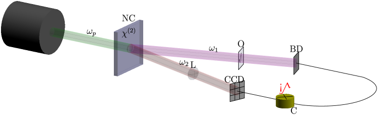
Figure 1: Usual ghost imaging setup. NC is a nonlinear crystal, $\omega_{p}$ is pump radiation, $\omega_{1}$ and $\omega_{2}$ are beams of entangled photon pairs (the beams diverge due to use of noncollinear parametric scattering), O is the object, BD is the bucket detector in the object arm, L is a converging lens, CCD is a photodetector array in the reference arm, C is an intensity correlator

1 The proposed imaging setup

We propose a new setup that provides, on one hand, preservation of the studied object by lowering illumination intensity, and on the other hand, improvement of image quality. The improvement of the signal-to-noise ratio, characteristic of ghost images formed by coincidence circuits, remains in force, i. e. it is possible to combine the advantages of ghost imaging with the advantages of ordinary imaging.

Consider fig. 2. The object arm has a detector array instead of a bucket detector, similarly to the reference arm. An ordinary image is formed on the array using an optical lens. Alternatively, in the case of X-ray illumination the array is placed immediately behind the object, as only reflective optical systems with large incidence angles work well enough in the X-ray range.

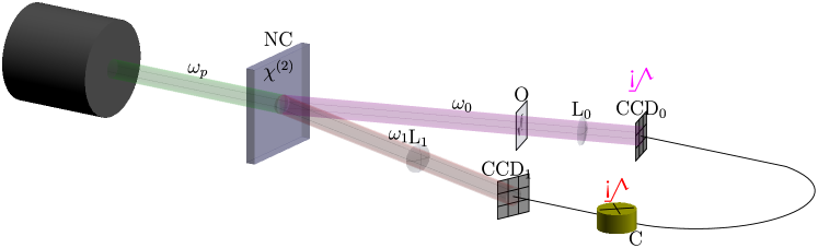
Figure 2: The proposed setup to produce a pair of quantum images. NC is a nonlinear crystal, $\omega_{p}$ is pump radiation, $\omega_{1}$ and $\omega_{2}$ are beams of entangled photon pairs (the beams diverge due to use of noncollinear parametric scattering), O is the object, L₀ and L₁ are optical lenses, CCD₀ and CCD₁ are photodetector arrays in object and reference arms, C is an intensity correlator

Hence, in the proposed setup, two images, an ordinary one and a quantum one, are produced. Their computer processing allows to lower the minimum number of illumination photons and to improve the image quality. Note that the proposed setup differs from difference measurements (see, e. g. [2]), as unlike them the acquired images are processed not by taking their difference. This means, in particular, that the requirement of identity of the sensors in object and reference arms is lifted. Furthermore, by virtue of radically different principles of our setup and the setup of difference measurements, the layouts of setups differs as well.

2 Measurement reduction method

The mathematical methods and algorithms for processing image(s) of an object that is illuminated by a low number of photons have to, in addition to providing maximal precision, enable use of all information about the object that is available to the researcher. The mathematical method of measurement reduction and its algorithmic implementations allow to achieve this.

Consider a typical measurement setup, in which the measured signal $f$ belonging to a Euclidean space $\mathcal{F}$, see [3], is formed at the input of a measuring transducer (MT). The MT transforms $f$ into a signal

$$\xi=Af+\nu,$$ (1)

that belongs to the Euclidean space $\mathcal{X}$, where $A\colon\mathcal{F}\to\mathcal{X}$ is the operator that models physical processes in the MT defining the transformation of $f$ into the signal $Af$ and denotes the modeled MT, $\nu$ is the measurement error. The measurement result depends on the characteristics of the measured object that interacts with the MT and is distorted by the measurement, while the researcher is usually interested in the characteristics of the object undistorted by the measurement. Their relation is modeled by an ideal MT that is given by the operator $U\colon\mathcal{F}\to\mathcal{U}$. The ideal MT transforms the same signal $f$ into the signal $Uf$ representing the features of interest to the researcher of the research object. The reduction problem consists of finding the reduction operator $R_{*}$ for which $R_{*}\xi$ is the most accurate version of $Uf$. If in (1) $f$ is an a priori arbitrary vector, $\nu$ is a random vector taking values in $\mathcal{X}$ that has expectation $\operatorname{\mathsf{E}}\nu=0$ and a non-degenerate covariance operator $\Sigma_{\nu}$: $\forall x\in\mathcal{X}$ $\Sigma_{\nu}x=\operatorname{\mathsf{E}}\nu(x,\nu)$, the linear reduction operator $R_{*}\colon\mathcal{X}\to\mathcal{U}$ is defined as the one minimizing the worst-case (in $f$) mean squared error (MSE) of interpreting $R\xi$ as $Uf$:

$$h(R,U)=\sup_{f\in\mathcal{F}}\lVert R\xi-Uf\rVert^{2}.$$

The MSE is minimal [3] for

$$R_{*}=U(A^{*}\Sigma_{\nu}^{-1}A)^{-1}A^{*}\Sigma_{\nu}^{-1}$$ (2)

and is equal to

$$h(R_{*},U)=\operatorname{tr}U(A^{*}\Sigma_{\nu}^{-1}A)^{-1}U^{*},$$ (3)

where ^- denotes pseudoinversion (Moore–Penrose inversion), if $U(I-A^{-}A)=0$, and is infinite otherwise.

Suppose that the researcher is interested in the transmittance distribution of the object. The values of pixel transmittances belong to the unit range. This is taken into account during measurement reduction by projecting the estimate onto the set $[0,1]^{\dim\mathcal{U}}$ [4, 5, 6]: the estimate is the fixed point of the mapping that combines the linear reduction result $R_{*}\xi$ and some estimate $\hat{u}$ of the transmittance distribution as uncorrelated results of the “main” and dummy measurements with subsequent projection onto $[0,1]^{\dim\mathcal{U}}$ while the minimized distance is the Mahalanobis distance $\lVert\Sigma_{R_{*}\xi}^{-1/2}\cdot\rVert$ that is induced by the covariance operator $\Sigma_{R_{*}\xi}=U(A^{*}\Sigma_{\nu}^{-1}A)^{-1}U^{*}$ of the linear reduction estimate. In addition, the researcher knows that transmittances of neighbouring pixels usually do not differ much. This information is formalized [7, 8, 9, 10, 11] by sparisty of the transmittance distribution as a vector $Uf$ in a given basis, i. e. as the information that in this basis most components of $Uf$ are zero. In [12, 13], an algorithm of measurement reduction that allows to take such information into account when processing multiplexed quantum ghost images was proposed. The algorithm is based on testing statistical hypotheses that estimate components in the chosen basis are zero (alternative hypotheses are that the components are non-zero). Testing results depend on the algorithm parameter $\tau$ that is related to the significance level of the used criterion. Its choice is determined by the compromise between noise suppression and image distortion that is acceptable to the researcher. Distortion is understood as a deterministic (as opposed to the noise) change during processing that brings the image away from the ideal one.

3 Effects of detector quantum efficiency on the measurement setup

Suppose that CCD arrays in object and reference arms are identical and are described by the operator $A_{0}$. In the case of unit quantum efficiency of the detectors the measurement setup (1) is as follows:

$$\xi=\begin{pmatrix}\xi_{0}\\ \xi_{1}\end{pmatrix}=\begin{pmatrix}A_{0}\\ A_{0}\end{pmatrix}nf+\begin{pmatrix}\nu_{\textnormal{img}}+\nu_{\epsilon}\\ \nu_{\textnormal{img}}\end{pmatrix},$$

where $\xi_{0}$ is the result of the measurement by the CCD array in the object arm, $\xi_{1}$ is the measured obtained ghost image, $\nu_{\textnormal{img}}$ is the part of error caused by quantum image acquisition, $\nu_{\epsilon}$ is the part of error of the quantum image acquired in the object arm that is caused by noise photons (during ghost imaging they are mostly suppressed by the coincidence circuit if its trigger time is sufficiently small, see comparison of quantum imaging setups in [7]; otherwise a similar term appears in the error of the acquired quantum ghost image), $n$ is the mean number of photons illuminating the object. The error covariance operator has the form

$$\Sigma_{\nu}=\begin{pmatrix}A_{0}S(f)A_{0}^{*}+\Sigma_{\nu_{\epsilon}}&A_{0}S(f)A_{0}^{*}\\ A_{0}S(f)A_{0}^{*}&A_{0}S(f)A_{0}^{*}\end{pmatrix}=\begin{pmatrix}1&1\\ 1&1\\ \end{pmatrix}\otimes A_{0}S(f)A_{0}^{*}+\begin{pmatrix}\Sigma_{\nu_{\epsilon}}&0\\ 0&0\end{pmatrix}$$ (4)

where the operator $S(f)$ is determined by photocount variances and covariances. For example, if photocounts are Poissonian, $S(f)=n\operatorname{diag}(f)$. Here and below $\operatorname{diag}(q)$ denotes the matrix whose diagonal elements are equal to corresponding components of $q$ and offdiagonal elements are zero, and $\otimes$ denotes Kronecker product. In this case acquisition of spatial intensity distribution in the object arm does not allow to improve reduction MSE (the reduction result does not depend on the result of the measurement in the object arm).

For object arm detector efficiency $\eta_{0}$ and reference arm detector efficiency $\eta_{1}$ the measurement setup becomes

$$\xi=\begin{pmatrix}\xi_{0}\\ \xi_{1}\end{pmatrix}=\begin{pmatrix}\eta_{0}A_{0}\\ \eta_{0}\eta_{1}A_{0}\end{pmatrix}nf+\begin{pmatrix}\nu_{\textnormal{img}}+\nu_{0}+\nu_{\epsilon}\\ \nu_{\textnormal{img}}+\nu_{0}+\nu_{1}\end{pmatrix},$$

where the additional errors $\nu_{0}$ and $\nu_{1}$ are caused by missing of some photons by the sensors in object and reference arms, respectively. The error covariance operator becomes

$$\Sigma_{\nu}=\eta_{0}^{2}\begin{pmatrix}1&\eta_{1}\\ \eta_{1}&\eta_{1}^{2}\end{pmatrix}\otimes A_{0}S(f)A_{0}^{*}+\\ +\eta_{0}^{2}\begin{pmatrix}\Sigma_{\nu_{\epsilon}}&0\\ 0&0\end{pmatrix}+\begin{pmatrix}\eta_{0}(1-\eta_{0})&\eta_{0}(1-\eta_{0})\eta_{1}\\ \eta_{0}(1-\eta_{0})\eta_{1}&\eta_{0}\eta_{1}(1-\eta_{0}\eta_{1})\end{pmatrix}\otimes\operatorname{diag}(A_{0}f),$$ (5)

where the first two terms have the same origin as in (4), but are weakened by the decrease of the mean number of photocounts, and the last term is directly related to non-unit detector efficiency.

As the linear reduction operator has the form (2), while the reduction estimate MSE is equal to (3), the gain caused by image acquisition in the object arm is equal to

$$\eta_{0}^{-2}\operatorname{tr}U\left(\eta_{0}\eta_{1}^{-1}\left(A_{0}^{*}\left(\eta_{0}\eta_{1}A_{0}S(f)A_{0}^{*}+(1-\eta_{0}\eta_{1})\operatorname{diag}(A_{0}f)\right)^{-1}A_{0}\right)^{-1}\right.-\\ -\left.\left(\begin{pmatrix}A_{0}^{*}&\eta_{1}A_{0}^{*}\end{pmatrix}\Sigma_{\nu}^{-1}\begin{pmatrix}A_{0}\\ \eta_{1}A_{0}\end{pmatrix}\right)^{-1}\right)U^{*},$$ (6)

where the operator $\Sigma_{\nu}$ is defined by the expression (5). Fig. 3 shows the relative gain in mean number of illumination photons as a function of detector quantum efficiency and the relative mean number of noise photons (relative to the mean number of illumination photons when only the ghost image is acquired).

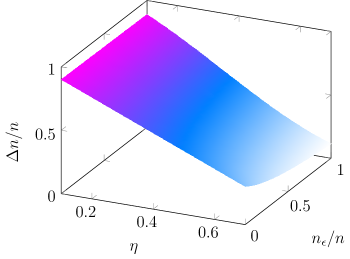
Figure 3: Relative gain $\Delta n/n$ in the mean number of illumination photons as a function of detector quantum efficiency $\eta=\eta_{0}=\eta_{1}$ and the relative mean number of noise photons $n_{\epsilon}/n$ (relative to the mean number of illumination photons $n$, when only the ghost image is acquired)

The gain is defined as the ration of the decrease $\Delta n$ in the mean number of photons that is required to illuminate the object to the mean number of illumination photons $n$ in the usual ghost imaging setup so that estimate MSE remains the same. It is expected that the number of noise photons decreases proportionally. As expected, the gain increases monotonically if the number of noise photons decreases or detector quantum efficiency $\eta=\eta_{0}=\eta_{1}$ decreases (in the figure we assume that detector efficiencies in both arms are equal). Without noise photons the relative gain is $1-\eta$. If additional information is available, the gain usually decreases while preserving its sign, as both compared MSEs decrease, but the greater one decreases more.

4 Computer modeling results

Fig. 4 shows the results of computer modeling and processing of quantum images using measurement reduction method via the algorithm described in [12, 13]. For modeling it was assumed that the CCD arrays in the arms are identical, the sensors are three times as large as an object pixel, each object pixel is illuminated by an average of $1$ photon, the mean number of noise photons that did not interact with the object but were detected by the sensor in the object arm is $0.1$ per pixel and detector quantum efficiencies are $0.4$.

As noted above, the algorithm parameter $\tau$ reflects a compromise between noise suppression and image distortion that is acceptable for the researcher. The larger the value of $\tau$, the larger noise suppression, but the distortion of image details increases as well (cf., e. g., figs. 4h and 4i, where increasing $\tau$ makes slit image mored blurred). The value $\tau=0$ corresponds to both absence of additional noise suppression using sparsity information about the transmittance distribution and absence of image distortion, i. e. it is equivalent to lack of information about the sparsity of object transmittance distribution. The values of $\tau$ shown in fig. 4 are chosen so that in fig. 4e the distortions are not be noticeable yet, and in fig. 4f they are be noticeable.

a Research object transmittance distribution

b The image acquired by the CCD array in the object arm

c The ghost image (GI)

d Reduction, no sparsity information

e Reduction with sparsity information, $\tau=0.1$

f Reduction with sparsity information, $\tau=0.2$

g GI reduction, no sparsity information

h GI reduction with sparsity information, $\tau=0.1$

i GI reduction with sparsity information, $\tau=0.2$

Figure 4: Quantum images of (4a) the object that were acquired in (4b) object and (4c) reference arms and the results of their processing using measurement reduction technique: the results of processing both images (4d) without using sparsity information and (4e, 4f) with using sparsity information for two values of the algorithm parameter $\tau$; (4g–4i) the results of processing only the ghost image using the same methods

The above suggestion that if additional information is available, the gain caused by processing the image acquired in the object arm decreases while preserving its sign is supported by the comparison of pairs of figs. 4d and 4g and figs. 4e and 4h: the former two differ more than the latter two, as the set of possible estimate values is restricted.

The estimate built on only the ghost image is more noisy than the estimate build on both images. Therefore, the blurring for the same values of the algorithm parameter $\tau$ that is responsible for the balance between blurring of important image details and noise suppression is larger for the estimate that uses only the ghost image.

Finally, the localization of the noise caused by the image acquired in the object arm differs from the localization of the noise caused by non-unit detector quantum efficiency. While the spatial distribution of noise caused by noise photons usually is independent of the object, the distribution of the noise caused by detector inefficiency is directly related to it, since the larger the number of the arrived photons, the larger the variance of the number of photocounts. For that reason the change of the parameter $\tau$ affects distortion of image details differently for areas with different average brightness.

Conclusion

In conclusion, we note that the considered imaging setup allows to improve the quantum image quality during computer processing step also by taking diffraction limits of ghost imaging into consideration in this step [14, 15, 16]. This is caused by the absence of diffraction limits on ordinary imaging that are inherent in ghost imaging and are related to limits on transversal pump size and, consequently, its divergence.

In addition, we would like to note an interesting setup based on the proposed one: simultaneous illumination of two objects that are located in different arms. In this way, 2 pairs of images (2 ordinary images and 2 ghost images) are produced at the same time at the cost of worsening the quality compared to absence of the second object. The cause of worsening is that the second object does not transmit some of the photons that are correlated with photons in the arm of the first object and vice versa. Nevertheless, this could be useful in some situations.

This work was supported by the Russian Foundation for Basic Research, project no. 18-01-00598 A.

References

- [1] Quantum imaging / Ed. by M. I. Kolobov. Springer New York, 2007.
- [2] Quantum noise in multipixel image processing / N. Treps, V. Delaubert, A. Maître et al. // Physical Review A. 2005. Vol. 71, no. 1. P. 013820.
- [3] Pyt’ev Yu. P. Methods of mathematical modeling of measuring–computing systems [in Russian]. 3 edition. Moscow : Fizmatlit, 2012.
- [4] Balakin D. A., Pyt’ev Yu. P. A comparative analysis of reduction quality for probabilistic and possibilistic measurement models // Moscow University Physics Bulletin. 2017. Vol. 72, no. 2. P. 101–112.
- [5] Balakin D. A., Pyt’ev Yu. P. Improvement of measurement reduction if the feature of interest of the research object belongs to a known convex closed set [in Russian] // Memoirs of the Faculty of Physics. 2018. no. 5. P. 1850301.
- [6] Balakin D. A., Belinsky A. V., Chirkin A. S. Improvement of the optical image reconstruction based on multiplexed quantum ghost images // Journal of Experimental and Theoretical Physics. 2017. Vol. 125, no. 2. P. 210–222.
- [7] Imaging with a small number of photons / P. A. Morris, R. S. Aspden, J. E. C. Bell et al. // Nat. Commun. 2015. Vol. 6. P. 5913.
- [8] Image quality enhancement in low-light-level ghost imaging using modified compressive sensing method / X. Shi, X. Huang, S. Nan et al. // Laser Phys. Lett. 2018. Vol. 15, no. 4. P. 045204.
- [9] Gong W., Han S. High-resolution far-field ghost imaging via sparsity constraint // Sci. Rep. 2015. Vol. 5, no. 1. P. 9280.
- [10] Entangled-photon compressive ghost imaging / P. Zerom, K. W. C. Chan, J. C. Howell, R. W. Boyd // Phys. Rev. A. 2011. Vol. 84, no. 6. P. 061804.
- [11] Katz O., Bromberg Y., Silberberg Y. Compressive ghost imaging // Appl. Phys. Lett. 2009. Vol. 95, no. 13. P. 131110.
- [12] Balakin D. A., Belinsky A. V. Reduction of multiplexed quantum ghost images // Moscow University Physics Bulletin. 2019. Vol. 74, no. 1. P. 8–16.
- [13] Balakin D. A., Belinsky A. V., Chirkin A. S. Object reconstruction from multiplexed quantum ghost images using reduction technique // Quantum Information Processing. 2019. Vol. 18, no. 3. P. 80.
- [14] Belinsky A. V. The “paradox” of Karl Popper and its connection with the heisenberg uncertainty principle and quantum ghost images // Moscow University Physics Bulletin. 2018. Vol. 73, no. 5. P. 447–456.
- [15] Experimental Limits of Ghost Diffraction: Popper’s Thought Experiment / P.-A. Moreau, P. A. Morris, E. Toninelli et al. // Scientific Reports. 2018. Vol. 8, no. 1. P. 13183.
- [16] Resolution limits of quantum ghost imaging / P.-A. Moreau, E. Toninelli, P. A. Morris et al. // Optics Express. 2018. Vol. 26, no. 6. P. 7528.