Supermassive black holes with high accretion rates in active galactic nuclei: X. Optical variability characteristics

Abstract

We compiled a sample of 73 active galactic nuclei (AGNs) with reverberation mapping (RM) observations from RM campaigns including our ongoing campaign of monitoring super-Eddington accreting massive black holes (SEAMBHs). This sample covers a large range of black hole (BH) mass $(M_{\bullet}=10^{6-9}~{}M_{\odot})$, dimensionless accretion rates $(\dot{\mathscr{M}}=10^{-2.7}-10^{2.7})$ and 5100 Å luminosity $(L_{5100}=10^{42-46}~{}\rm erg~{}s^{-1})$, allowing us to systematically study the AGN variability and their relations with BH mass, accretion rates, and optical luminosity. We employed the damped random walk (DRW) model to delineate the optical variability of continuum at 5100 Å and obtained damped variability timescale ($\tau_{\rm d}$) and amplitude ($\sigma_{\rm d}$) using a Markov Chain Monte Carlo (MCMC) method. We also estimated the traditional variability amplitudes ($F_{\rm var}$), which provide a model-independent measure and therefore are used to test the DRW results. We found that AGN variability characteristics are generally correlated with $(M_{\bullet},\dot{\mathscr{M}},L_{5100})$. These correlations are smooth from sub-Eddington to super-Eddington accretion AGNs, probably implying that the AGN variability may be caused by the same physical mechanism.

1 Introduction

Accretion onto supermassive black holes (BHs) is commonly believed to be the powerful energy source of active galactic nuclei (AGNs; e.g., Rees 1984), which is evidenced by the prominent big blue bumps in AGN spectrum energy distributions (e.g. Shields 1978; Malkan 1983;Ho 2008). However, the detailed physics of accretion disks are still insufficiently understood, even for the basic process of energy dissipation (Lawrence 2018). AGNs have long been known to show aperiodic variability across a broad wavelength band from radio to X-ray at various time scales, which delivers useful information on emissions from accretion disk (Ulrich et al. 1997). Many previous works studied optical variability of AGNs based on various samples (Giveon et al., 1999; MacLeod et al., 2010; Zuo et al., 2012; Lu et al., 2016b) and made great efforts to investigate the relationships between variability characteristics and AGN properties, such as, optical luminosity, BH mass, and Eddington ratio (e.g., Sánchez-Sáez et al. 2018; Rakshit & Stalin 2017; Wold et al. 2007; Wilhite et al. 2008; Bauer et al. 2009; Zuo et al. 2012; Hook et al. 1994; Cristiani et al. 1997; Giveon et al. 1999; Hawkins 1996; Vanden Berk et al. 2004).

Spectroscopic monitoring campaigns have successfully probed geometry and kinematics of the broad-line region (BLR), but also have accumulated precious variability databases. The major advantage of RM databases is that the AGN properties, such as BH mass and accretion rate, can be more reliably estimated. In addition, the quality of light curves from RM campaigns (e.g., sampling and measurement accuracy) is generally better than that from other time-domain surveys (except for some light curves observed by the Kepler telescope). In 2012, we started a long-term RM campaign aiming at monitoring super-Eddington accreting massive black holes (SEAMBHs) using the Lijiang 2.4m telescope (Du et al. 2014; Du et al. 2018). By combining with RM AGNs from previous RM campaigns (e.g., Bentz et al. 2013), there are $\sim$100 AGNs monitored by RM campaigns. This sample provides with us a good opportunity to study AGN variability characteristics, and their connections with AGN basic properties (BH mass, accretion rates, and optical luminosity).

The paper is organized as follows. We describe the sample and AGN properties in Section 2. Section 3 presents the methodology and variability characteristics of AGNs. We test the validity of the DRW model in Section 4, and investigate the differences of variability characteristics between super- and sub-Eddington accretion AGNs in Section 5. Section 6 performs a correlation analysis between variability characteristics and AGN properties. We draw our conclusion in Section 7.

2 Sample and Properties

For the purpose of accurately determining the BH mass and accretion rates, we only selected AGNs with RM observations that detect significant H$\beta$ time delays. Over the past 30 years, great efforts have been made to conduct RM monitoring of nearby AGNs (e.g., Peterson et al. 1998; Kaspi et al. 2000; Bentz et al. 2013; Denney et al. 2009; Grier et al. 2012). Du et al. (2015) compiled all the published RM measurements before the year of 2014 (see Table 7 of Du et al. 2015), and most of the mapped AGNs before 2013 are sub-Eddington AGNs. Recently, the SDSS-RM project monitored a sample of AGNs with redshift up to $z\sim 0.3$ (Shen et al. 2015; Grier et al. 2017), but their database is not available. The SEAMBH project provided a complementary sample of super-Eddington accretion AGNs, and the latest SEAMBH results are reported in paper of Du et al. (2016, 2018). We finally obtain a sample of 73 AGNs with 113 light curves (because some objects have multiple RM campaigns, such as NGC 5548 and Mrk 335). The light curves do not include the component of the broad-emission line since they were measured from the optical spectra at 5100 Å  (for references see column 11 of Table 1). For these objects observed with multiple campaigns, we do not combine their measurements but instead treat the measurements independently in the following analysis. It should be noted that AGN luminosity at 5100 Å is contaminated by emission from stars in the host galaxy, especially, the host to optical luminosity ratio ($L_{\rm host}/L_{\rm opt}$) maybe larger than 50% in low-luminosity AGNs (see Figure 13 of Stern & Laor 2012). In our sample, the optical luminosity $L_{5100}$ has been corrected for the starlight of the host galaxy either by HST data or empirical relation (see Bentz et al. 2013; Du et al. 2015, 2018), in which the characteristic ratio of host to optical luminosity is $L_{\rm host}/L_{\rm opt}=0.41$ with a scatter of 0.21. This larger scatter is consistent with the fact that the host to AGN luminosity (e.g., $L_{\rm 5100}$) ratio is a function of AGN bolometric luminosity (Shen et al., 2011; Stern & Laor, 2012). Table 1 summarizes the basic properties of the sample.

With the usual assumption that motion of the BLR clouds is virialized, we estimate BH mass by

$$M_{\bullet}=f_{\scriptscriptstyle\rm BLR}\frac{V_{\rm BLR}^{2}R_{\scriptscriptstyle{\rm BLR}}}{G},$$ (1)

where $R_{\scriptscriptstyle{\rm BLR}}=c\tau_{{}_{\rm H\beta}}$, $\tau_{{}_{\rm H\beta}}$ is the H$\beta$ time lag with respective to the 5100 Å continuum, $G$ is the gravitational constant, $c$ is the speed of light, and $f_{\scriptscriptstyle\rm BLR}$ is the so-called virial factor that includes all the unknown information about the geometry and kinematics of the BLR gas. The dimensionless accretion rate is related to the 5100 Å  luminosity and BH mass via (Du et al., 2014)

$$\dot{\mathscr{M}}=\frac{\dot{M}_{\bullet}}{L_{\rm Edd}c^{-2}}=20.1\left(\frac{\ell_{44}}{\cos i}\right)^{3/2}M_{7}^{-2},$$ (2)

where $\dot{M}_{\bullet}$ is the accretion rates, $\ell_{44}=L_{5100}/10^{44}\rm erg~{}s^{-1}$, $M_{7}=M_{\bullet}/10^{7}M_{\odot}$ is the BH mass, and $\cos i$ is the cosine of the inclination of the accretion disk. Following the usual approximation, we take $\cos i=0.75$, corresponding to an inclination angle of $\sim 40^{\circ}$.

Figure 1 shows the distributions of redshifts ($z$), 5100 Å luminosity ($L_{\rm 5100}$), BH mass ($M_{\bullet}$), and dimensionless accretion rates ($\dot{\mathscr{M}}$) of our sample. Following Du et al. (2015), we classify AGNs into sub-Eddington and super-Eddington regimes by $\dot{\mathscr{M}}=3$, beyond which the inner parts of disk break the standard model of accretion disk (Laor & Netzer, 1989), the radial advection of accrete flows is not negligible. The AGNs with high accretion rates ($\dot{\mathscr{M}}\gtrsim 3$) are thought to be powered by slim disk (Abramowicz et al., 1988). We have a number ratio of the two subsamples $N_{\dot{\mathscr{M}}\geq 3}:N_{\dot{\mathscr{M}}<3}=48:65$, implying that the entire sample covers a homogeneous range of accretion rates.

Here we would like to point out the difference between $\dot{\mathscr{M}}$ and Eddington ratios defined by $\lambda_{\rm Edd}=L_{\rm Bol}/L_{\rm Edd}$, where $L_{\rm Bol}$ is the bolometric luminosity. In the Shakura-Sunyaev regime (Shakura & Sunyaev, 1973), we have $L_{\rm Bol}=\eta\dot{M}_{\bullet}c^{2}$, where $\eta$ is the radiative efficiency depending on BH spins. We have $\lambda_{\rm Edd}=\eta\dot{\mathscr{M}}$ from Equation (2), that is $\dot{\mathscr{M}}$ is linearly proportional to $\lambda_{\rm Edd}$, indicating that $\dot{\mathscr{M}}$ and $\lambda_{\rm Edd}$ represent the accretion rates in sub-Eddington accreting AGNs. However, $\lambda_{\rm Edd}$ cannot be an indicator of accretion rates in super-Eddington AGNs. Beyond the Shakura-Sunyaev model, the slim accretion disk is characterized by its fast radial motion compared with Keplerian rotation giving rise to nonlocal energy budget. In this case, photons produced in the viscose dissipation are trapped inside accretion flow so that a large fraction of photons are swallowed into the BH before they escape from the disk surface. This photon trapping effect leads to that the radiated luminosity ($L_{\rm Bol}$) being saturated when $\dot{\mathscr{M}}\gg 1$ (see Figure 1 of Abramowicz et al. 1988 or Figure 2 of Mineshige et al. 2000). In such a case, $\lambda_{\rm Edd}\sim 1$, but $\dot{\mathscr{M}}\gg 1$, indicating that Eddington ratios cannot represent accretion rates in super-Eddington AGNs. Earlier discussions on the validity of the Shakura-Sunyaev disk show that geometrically thin approximation is broken for $\dot{\mathscr{M}}\gtrsim 3$ (see details in Laor & Netzer, 1989) extending to the regime of slim disk (Wang et al., 2014). We thus take this approach in this paper.

Moreover, applying the $R-L$ relation and its lines extended to Mg ii and C iv, astronomers estimated Eddington ratios of a large sample, such as the Sloan Digital Sky Survey (SDSS) (e.g., McLure & Jarvis, 2002; Shen et al., 2011), the AGN and Galaxy Evolution Survey (AGES) (Kollmeier et al., 2006), where the bolometric correction factor is usually taken to be about 10. This factor is too small for some AGNs (Jin et al., 2012). They found $\lambda_{\rm Edd}\lesssim 1$ in quasars. The long-term ongoing SEAMBH campaign is getting more evidence for shortened H$\beta$ lags for optical Fe ii strong AGNs (Du et al., 2015, 2016, 2018), implying that BH masses in some quasars are overestimated and Eddington ratios are underestimated. Estimations of BH mass and Eddington ratios need to be improved.

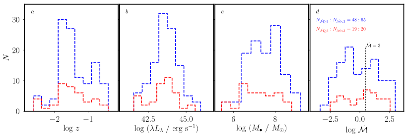
Figure 1: The distributions of AGN properties: (a) redshift, (b) optical luminosity, (c) black hole mass, and (d) accretion rates. Blue dashed-line is for all RM AGNs and red dashed-line is for the AGNs with $\tau_{\rm d}|_{<0.1D}$ (see Section 4).

3 Methodology and Variability Characteristics

3.1 Damped Random Walk Model

Damped random walk (DRW) is a stochastic process, defined by an exponential covariance function (e.g., Zu et al. 2011, 2013),

$$S(t_{1},t_{2})=\sigma_{\rm d}^{2}\exp\left[-\left(\frac{|t_{i}-t_{j}|}{\tau_{\rm d}}\right)\right],$$ (3)

where $\tau_{\rm d}$ is the characteristic variability timescale in units of days, $t_{i}-t_{j}=\Delta t$ is the time sampling interval between the $i$th and $j$th observations, and $\sigma_{\rm d}$ is the characteristic variability amplitude in units of flux density. It has been shown that AGNs variability in the optical band can be well described by the DRW (e.g., Kelly et al. 2009; Kozłowski et al. 2010; MacLeod et al. 2010, 2011; Zu et al. 2013;Rakshit & Stalin 2017). The model has been widely used in modeling AGN light curves in reverberation mapping (RM) studies (see Zu et al. 2011; Pancoast et al. 2011; Grier et al. 2012; Li et al. 2013; Zhang et al. 2018). The limitations of the DRW model in describing AGN variability characteristics will be discussed in Section 4.

The framework for estimating DRW model parameters and reconstructing AGN light curves has been well-established, e.g, see Rybicki & Press (1992) and Zu et al. (2011). Here we briefly list the essential points for the sake of completeness. Following Rybicki & Press 1992, we model light curves as

$$\mathbi{y}=\mathbi{s+n}+\mathbi{E}\mathbi{q},$$ (4)

where $\mathbi{s}$ is the underlying variability signal with covariance matrix $\mathbi{S}$, $\mathbi{n}$ is the measurement errors with covariance matrix $\mathbi{N}$, $\mathbi{E}$ is a vector with all unity elements (i.e. $E_{i}=1$), and $\mathbi{q}$ is the mean value in the light curves. The overall covariance matrix of data is $\mathbi{C}=\mathbi{S}+\mathbi{N}$. The posterior probability of the observed data for a given set of DRW model parameters is (Zu et al., 2011; Kozłowski et al., 2010)

$$P(\mathbi{y}|\sigma_{\rm d},\tau_{d})\propto\mathcal{L}\equiv|\mathbi{C}|^{-1/2}|\mathbi{E}^{T}\mathbi{C}^{-1}\mathbi{E}|^{-1/2}\exp\left(-\frac{1}{2}\mathbi{y}^{T}\mathbi{C}_{\perp}^{-1}\mathbi{y}\right),$$ (5)

where

$$\mathbi{C}_{\perp}^{-1}=\mathbi{C}^{-1}-\mathbi{C}^{-1}\mathbi{E}(\mathbi{E}^{T}\mathbi{C}^{-1}\mathbi{E})\mathbi{E}^{T}\mathbi{C}^{-1}.$$ (6)

We maximize the posterior probability to determine the best estimate of $\sigma_{\rm d}$ and $\tau_{d}$ and their uncertainties.

After determining the values of $\sigma_{\rm d}$ and $\tau_{\rm d}$, an unbiased estimate of the light curve at time $t_{\ast}$ is (Rybicki & Press, 1992)

$$\widehat{y_{\ast}}=\mathbi{S}_{\ast}^{T}\mathbi{C}^{-1}\mathbi{(y-E}\hat{q})+\hat{q}.$$ (7)

The mean square residual of this estimate is (Li et al., 2013)

$$\langle(y_{\ast}-\widehat{y_{\ast}})^{2}\rangle=\langle y_{\ast}^{2}\rangle-\mathbi{S}_{\ast}^{T}\mathbi{C}^{-1}\mathbi{S_{\ast}}+\frac{(\mathbi{S}_{\ast}^{T}\mathbi{C}^{-1}\mathbi{E}-1)^{2}}{\mathbi{E}^{T}\mathbi{C}^{-1}\mathbi{E}}.$$ (8)

3.2 Intrinsic Variability Amplitude

The widely used variability amplitude of an AGN light curve is defined as (Rodriguez-Pascual et al. 1997)

$$F_{\rm var}=\frac{\left(\sigma^{2}-\Delta^{2}\right)^{1/2}}{\langle F\rangle}\,.$$ (9)

The uncertainty of $F_{\rm var}$ is defined as (see Edelson et al. 2002),

$$\sigma_{{}_{F_{\rm var}}}=\frac{1}{F_{\rm var}}\left(\frac{1}{2N}\right)^{1/2}\frac{\sigma^{2}}{\langle F\rangle},\quad\sigma^{2}=\frac{1}{N-1}\sum_{i=1}^{N}\left(F_{i}-\langle F\rangle\right)^{2},$$ (10)

where $\langle F\rangle=N^{-1}\sum_{i=1}^{N}F_{i}$ is the average flux, $N$ is the number of observations, $\Delta^{2}=\sum_{i=1}^{N}\Delta_{i}^{2}/N$, $\Delta_{i}$ represents the uncertainty on the flux $F_{i}$. $F_{\rm var}$ gives an estimate of the relative intrinsic variability amplitude by accounting for the measurement uncertainties.

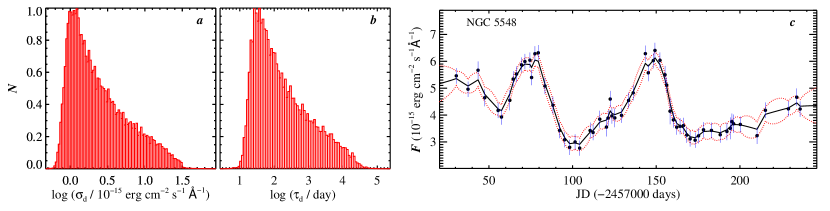
Figure 2: Estimates for the DRW model parameters and a reconstruction of light curve for NGC 5548 from Lu et al. (2016a). Panels (a, b) show the posterior distributions of $\sigma_{\rm d}$ and $\tau_{\rm d}$ constructed from an MCMC method. The distributions were normalised by the peak values. In Panel (c), the points with error bars represent the observed data. The solid line represents the best reconstruction and the dashed lines represent the 1$\sigma$ uncertainties.

3.3 Variability Characteristics

To estimate the DRW model parameters $\sigma_{\rm d}$ and $\tau_{\rm d}$ in Equation (3), we employed the Markov Chain Monte Carlo (MCMC) method and the Metropolis-Hastings algorithm to construct a sample from the posterior probability distribution. By maximizing the posterior probability distribution (Equation 5), we obtain the best estimates of $\sigma_{\rm d}$ and $\tau_{\rm d}$. In Figure 2, we take a light curve of NGC 5548 as an example and apply the DRW model. Panels (a) and (b) of Figure 2 show the posterior distributions of $\sigma_{\rm d}$ and ($\tau_{\rm d}$), respectively. We take the best estimates of $\sigma_{\rm d}$ and $\tau_{\rm d}$ to be the peak location of the distributions and the uncertainties to be the 68.3% confidence interval. The underlying signal of light curves can be reconstructed using the best estimates of $\sigma_{\rm d}$ and $\tau_{\rm d}$. Panel (c) of Figure 2 shows the best reconstruction (solid line) of the light curve of NGC 5548. In the next analysis, we normalized $\sigma_{\rm d}$ using average flux of light curve and called it as $\Sigma_{\rm d}$ (i.e. $\frac{\sigma_{\rm d}}{\langle F\rangle}$, where $\langle F\rangle$ is average flux of light curves). The values of $\Sigma_{\rm d}$, $\tau_{\rm d}$, $F_{\rm var}$ and $R_{\rm max}$ for all RM AGNs are tabulated in Table 1.

4 Test Validity of DRW Parameters

The previous studies based on Kepler observations found that the AGN light curves may deviate from the DRW model and concluded that AGN variability is so complex that more sophisticated models are required (Mushotzky et al., 2011; Kasliwal et al., 2015). To explore possible deviations, Zu et al. (2013) considered a set of AGN variability models and found that the light curves of the OGLE quasar are well described by the DRW model. Studying the influences of light-curve length, magnitude, and cadence on recovering the DRW model parameters, Kozłowski (2017) found that the light curves without enough time length cannot reliably constrain damped variability timescale, and suggested that the time length of light curves must be at least 10 times longer than the true damped variability timescale. Based on this point, we divided all RM AGNs into two subsamples, they are (1) the $\tau_{\rm d}|_{<0.1D}$ sample in which the damped variability timescales are less than 10% of the observation length of light curves (including 39 measurements, where ‘$D$’ means the observation length of light curves), and (2) the $\tau_{\rm d}|_{\geq 0.1D}$ sample in which the damped variability timescales are greater than or equal to 10% of the observation length of light curves (including 74 measurements). After comparing the damped variability amplitude ($\Sigma_{\rm d}$, model-dependent) with intrinsic variability amplitude ($F_{\rm var}$, model-independent), we found that $\Sigma_{\rm d}$ is approximately equal to $F_{\rm var}$ in the $\tau_{\rm d}|_{<0.1D}$ sample (see Figure 3), but deviate from $F_{\rm var}$ in the $\tau_{\rm d}|_{>0.1D}$ sample.

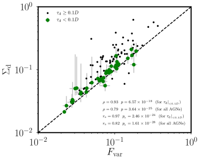
Figure 3: Comparison between the damped variability amplitude and intrinsic variability amplitude. The number ratio of $\tau_{\rm d}|_{<0.1D}$ AGNs (in green) and $\tau_{\rm d}|_{\geq 0.1D}$ AGNs (in black) is 39:74. The dashed line presents $\Sigma_{\rm d}=F_{\rm var}$. ($\rho,p$) and ($r_{\rm s},p_{\rm s}$) are the results of the Pearson correlation and Spearman’s rank correlation analysis, respectively.

We employed the Pearson correlation and Spearman’s rank correlation analysis to quantitatively compare the relation between $\Sigma_{\rm d}$ and $F_{\rm var}$ of two subsamples, the results were shown in Figure 3. We found that $\Sigma_{\rm d}$ is linearly correlated with $F_{\rm var}$ in the $\tau_{\rm d}|_{<0.1D}$ sample. However, if we included the $\tau_{\rm d}|_{\geq 0.1D}$ sample (plotted in black dots), $\Sigma_{\rm d}$ gradually deviates from $F_{\rm var}$. We further performed a linear regression using the LinMix method (Kelly 2007) for $\tau_{\rm d}|_{<0.1D}$ sample. The regression method assumes: $y=\alpha+\beta x+\epsilon$, where $\epsilon$ is the intrinsic scatter about the regression. The regression analysis gives

$$\log\Sigma_{\rm d}=(0.09\pm 0.07)+(1.05\pm 0.06)\log F_{\rm var}~{}~{}({\rm for}~{}\tau_{\rm d}|_{<0.1D}),$$ (11)

with intrinsic scatter of $\epsilon=0.03$. These checks confirm the suggestion that the DRW model can return reliable DRW model parameters if the observation length of light curves is 10 times longer than the true damped variability timescale (i.e. $D>10~{}\tau_{\rm d}$, see Kozłowski 2017). Therefore, to obtain reasonable results, we only used the AGNs with $\tau_{\rm d}<0.1D$ to investigate the variability characteristics in the following analysis. In the statistical analysis of variability amplitudes $F_{\rm var}$ and $R_{\rm max}$, we included the objects with $\tau_{\rm d}\geq 0.1D$ in the sample because they are model-independent variability amplitudes. The distributions of AGN physical properties ($z$, $L_{5100}$, $M_{\bullet}$, and $\dot{\mathscr{M}}$) of the $\tau_{\rm d}|_{<0.1D}$ sample are plotted (red dashed line) in Figure 1, which gives a number ratio $N_{\dot{\mathscr{M}}\geq 3}:N_{\dot{\mathscr{M}}<3}=19:20$.

In addition, based on 1384 variable AGNs from the QUEST-La Silla AGN variability survey, Sánchez-Sáez et al. (2018) found that the DRW variability amplitude is affected by the length of the light curve, and concluded that the variability of 74% of AGNs can be described by the DRW model in their defined sample. While, our analysis shows that only 35% (39$/$113) of light curves can be obtained with reliable DRW model parameters in RM AGNs. This percentage is significant lower than Sánchez-Sáez et al. (2018) results, which may be attributed to the fact that the light curves length ($\sim$ 1 yr) of the RM AGNs is shorter than Sánchez-Sáez et al. (2018) sample.

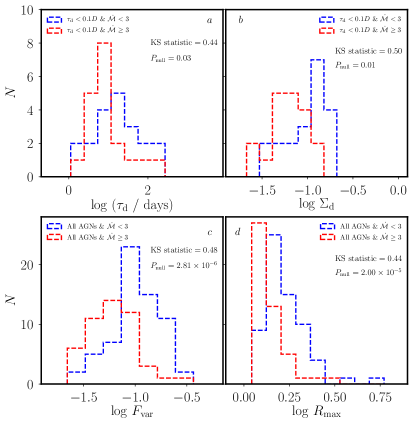
Figure 4: Distributions of variability characteristics. Panels (a) and (b) are DRW model parameters of $\tau_{\rm d}|_{<0.1D}$ sample. Panels (c) and (d) are intrinsic variability amplitude and flux ratio, which include all RM AGNs ($\tau_{\rm d}|_{<0.1D}$ and $\tau_{\rm d}|_{\geq 0.1D}$) since both parameters are model-independent.

5 Differences between Sub- and Super-Eddington Accreting AGNs

In this section, we investigate the differences of variability characteristics between sub-Eddington and super-Eddington accreting AGNs. Figure 4 plots the distributions of variability characteristics $\tau_{\rm d}$, $\Sigma_{\rm d}$, $F_{\rm var}$ and $R_{\rm max}$. To quantify the differences of variability characteristics between $\dot{\mathscr{M}}\geq 3$ and $\dot{\mathscr{M}}<3$ subsamples, we employed the Kolmogorov-Smirnov (KS) statistic test. The results were quoted in Figure 4. For DRW model parameters, we only plotted the distributions of $\tau_{\rm d}|_{<0.1D}$ AGNs. The KS statistic tests show that the distributions of DRW model parameters for $\dot{\mathscr{M}}\geq 3$ and $\dot{\mathscr{M}}<3$ subsamples are marginally different. For the model-independent variability parameters ($F_{\rm var}$ and $R_{\rm max}$), we plotted the distributions of all RM AGNs because they are model-independent. The KS statistic and the $P_{\rm null}$ show that the distributions of both $F_{\rm var}$ and $R_{\rm max}$ for $\dot{\mathscr{M}}\geq 3$ and $\dot{\mathscr{M}}<3$ subsamples are different. These results indicate that the $\dot{\mathscr{M}}\geq 3$ AGNs have lower variability amplitude ($F_{\rm var}$, $R_{\rm max}$ as well as $\Sigma_{\rm d}$) than the $\dot{\mathscr{M}}<3$ AGNs, which supports the previous notion that AGNs with high accretion rates have systematically low variability (e.g., Wilhite et al. 2008; Bauer et al. 2009; Zuo et al. 2012; Rakshit & Stalin 2017).

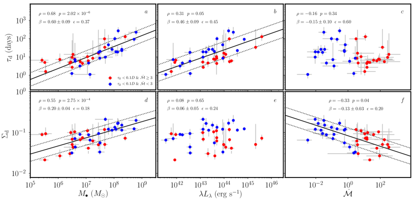
Figure 5: Dependence of DRW model parameters on AGN properties for $\tau_{\rm d}|_{<0.1D}$ sample. The top (a, b, c) and bottom (d, e, f) panels show the damped variability timescale and amplitude as a function of black hole mass, optical luminosity and the accretion rates, respectively. Solid lines are the best fit and dotted-lines show the intrinsic scatters. Red points are the AGNs with $\tau_{\rm d}<0.1D$ and $\dot{\mathscr{M}}\geq 3$, blue points are the AGNs with $\tau_{\rm d}<0.1D$ and $\dot{\mathscr{M}}<3$. The Pearson correlation coefficient $\rho$ and non-correlation probability $p$ are quoted. $\beta$ and $\epsilon$ are the slope and intrinsic scatter, respectively.

6 Correlation Analysis

6.1 Variability Characteristics and AGN Properties

In Figures 5 and 6, we plotted the model-dependent variability parameters and the intrinsic variability amplitude as a function of AGN properties, respectively. Then we calculated the Pearson correlation coefficient $\rho$ and noncorrelation probability $p$ between variability characteristics and AGN properties. All results are listed in Table 2. We also performed a linear regression using the LinMix method. The results of the linear regression for $\tau_{\rm d}$ are

$$(-3.24\pm 0.68)+(0.60\pm 0.09)\log M_{\bullet}~{}~{}({\rm for}~{}\tau_{\rm d}|_{<0.1D}),$$ (12a)

$$(-18.52\pm 4.06)+(0.46\pm 0.09)\log L_{5100}~{}~{}({\rm for}~{}\tau_{\rm d}|_{<0.1D}),$$ (12b)

with intrinsic scatters of $\epsilon=(0.37,0.45)$ for (12a, 12b), respectively. The results of the linear regression for $\Sigma_{\rm d}$ are

$$(-2.51\pm 0.31)+(0.20\pm 0.04)\log M_{\bullet}~{}~{}({\rm for}~{}\tau_{\rm d}|_{<0.1D}),$$ (13a)

$$(-1.08\pm 0.04)-(0.13\pm 0.03)\log\dot{\mathscr{M}}~{}~{}({\rm for}~{}\tau_{\rm d}|_{<0.1D}),$$ (13b)

with intrinsic scatters of $\epsilon=(0.18,0.20)$ for (13a, 13b), respectively. The results of the linear regression for $F_{\rm var}$ are

$$(-2.45\pm 0.34)+(0.18\pm 0.05)\log M_{\bullet}~{}~{}({\rm for}~{}\tau_{\rm d}|_{<0.1D}),$$ (14a)

$$(-1.13\pm 0.04)-(0.13\pm 0.03)\log\dot{\mathscr{M}}~{}~{}({\rm for}~{}\tau_{\rm d}|_{<0.1D}),$$ (14b)

$$(-2.32\pm 0.22)+(0.16\pm 0.03)\log M_{\bullet}~{}~{}({\rm for~{}all~{}AGNs}),$$ (14c)

$$(-1.08\pm 0.02)-(0.09\pm 0.02)\log\dot{\mathscr{M}}~{}~{}({\rm for~{}all~{}AGNs}),$$ (14d)

with intrinsic scatters of $\epsilon=(0.22,0.21,0.22,0.22)$ for (14a, 14b, 14c, 14d), respectively. From Equation (14), we found that the linear regression results between variability amplitude $F_{\rm var}$ and AGN parameters ($M_{\bullet},\dot{\mathscr{M}}$ and $L_{5100}$) for $\tau_{\rm d}|_{<0.1D}$ sample and all RM AGNs are consistent within the uncertainties. For the $\tau_{\rm d}|_{<0.1D}$ sample, because $\Sigma_{\rm d}$ is one-to-one correspondence with $F_{\rm var}$ (see Figure 3), their linear regression results with AGN properties ($M_{\bullet}$ and $\dot{\mathscr{M}}$) are consistent within the uncertainties (Equation 13 and 14). Because the variability amplitudes ($\Sigma_{\rm d}$ and $F_{\rm var}$) do not show significant correlation with optical luminosity (for $\Sigma_{\rm d}$: $\rho=0.08$, $p=0.65$; for $F_{\rm var}$: $\rho=0.11$, $p=0.55$), and damped variability timescales ($\tau_{\rm d}$) do not show significant correlation with accretion rates ($\rho=-0.16$, $p=0.34$, and $\beta=-0.15\pm 0.10$, $\epsilon=0.60$), we do not include its regression results in Equations (12), (13) and (14).

For $\tau_{\rm d}|_{<0.1D}$ AGNs, the results of correlation analysis (see Figures 5,  6 and Table 2) and linear regression (Equations 12, 13 and 14) between variability characteristics ($\tau_{\rm d}$, $\Sigma_{\rm d}$ and $F_{\rm var}$) and AGN properties show that:

1. Variability amplitudes ($\Sigma_{\rm d}$ and $F_{\rm var}$) do not significantly correlate with optical luminosity, which is consistent with the previous results (e.g., Bonoli et al. 1979; Giallongo et al. 1991; Cimatti et al. 1993; Netzer et al. 1996). Meanwhile, $\Sigma_{\rm d}$ and $F_{\rm var}$ increase with increasing black hole mass, which is similar to the results of Wold et al. (2007), Wilhite et al. (2008), and Bauer et al. (2009) but different from the findings of Simm et al. (2016) and Sánchez-Sáez et al. (2018), and they decrease with increasing accretion rates, which is consistent with recent results of Simm et al. (2016); Rakshit & Stalin (2017) and Sánchez-Sáez et al. (2018). The latter relation demonstrates that AGN optical fluctuations depend on accretion rates (also see Wold et al. 2007; Zuo et al. 2012; Rakshit & Stalin 2017).

2. MacLeod et al. (2010) modeled the variability of SDSS stripe 82 (S82) quasars using the DRW model and found that variability timescale increases with increasing black hole mass with a slope of $0.21\pm 0.07$, and is nearly independent on optical luminosity. However, in our $\tau_{\rm d}|_{<0.1D}$ sample, we found that damped variability timescale $\tau_{\rm d}$ increases with increasing black hole mass with a slope of $0.60\pm 0.09$, and with increasing optical luminosity with a slope of $0.46\pm 0.09$. Our results give more significant correlations between damped variability timescale and AGN properties than MacLeod et al. (2010). These results, constructed from the different databases, are not strictly consistent with each other, which may be attributed to the following reasons: 1) The sample size of S82 quasars is much larger than RM AGNs, but the light curves of RM AGNs have better sampling than S82 quasars. 2) The light curves of S82 quasars are the photometric data in the $ugriz$ band, which includes the contributions of the broad-emission line to some degree. Whereas, the light curves of RM AGNs were measured from the optical spectra at 5100 Å, which are not contaminated by broad-emission lines (see Section 2). 3) The physical properties of RM AGNs (see Section 2) could be more precise than S82 quasars. For example, virial BH masses of S82 quasars based on single-epoch spectra could include the scatter of the empirical relationship (e.g., the scatter of the latest Radius$-$Luminosity relation is larger than 0.3 dex, see Du et al. 2018).

3. For sub-Eddington or super-Eddington accretion AGNs, we found from the above relationships that the variability characteristics are generally driven by AGN properties in the same fashion. This probably indicates that the variability of AGNs powered by different accretion rates may be caused by the same physical mechanism.

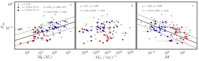
Figure 6: The same as Fig. 5, but for the relation between intrinsic variability amplitude and AGN properties. In panels, we included $\tau_{\rm d}|_{\geq 0.1D}$ sample (in black dot) since $F_{\rm var}$ is a model-independent variability amplitude, but only quoted the analysis results ($\rho$, $p$) and ($\beta$, $\epsilon$) of $\tau_{\rm d}|_{<0.1D}$ sample. We listed the correlation analysis results of all RM AGNs into Table 2, and wrote the regression results into Equation 14. We also only showed the best fit (solid lines) and intrinsic scatters (dotted-lines) of $\tau_{\rm d}|_{<0.1D}$ sample.

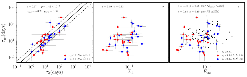
Figure 7: H$\beta$ time lag ($\tau_{\rm H\beta}$) as a function of damped variability timescale ($\tau_{\rm d}$), damped variability amplitude ($\Sigma_{\rm d}$) and model-independent amplitude ($F_{\rm var}$) from the left to right panels. In panel (a), we give the partial correlation coefficient $r_{\rm xy,z}=-0.20$ (where $x\equiv\tau_{\rm d}$, $y\equiv\tau_{\rm H\beta}$ and $z\equiv L_{5100}$) and null probability $p_{\rm xy,z}=0.06$. In panel (c), we over-plotted the $\tau_{\rm d}|_{\geq 0.1D}$ sample in black dot.

6.2 $\rm{H}\beta$ Lag and Variability Characteristics

In this section, we investigate the relationship between H$\beta$ time lag (i.e., radius of the BLR) and variability characteristics (see Figure 7). We found that H$\beta$ time lags do not significantly correlate with the variability amplitudes ($\Sigma_{\rm d}$ and $F_{\rm var}$), but significantly correlate with damped variability timescales ($\rho=0.57$, $p=1.43\times 10^{-4}$). By a linear regression analysis, we yield

$$\log\tau_{\rm H\beta}=(0.27\pm 0.13)+(0.76\pm 0.10)\log\tau_{{}_{\rm d}}~{}~{}({\rm for}~{}\tau_{\rm d}|_{<0.1D}).\$$ (15)

This relationship gives an intrinsic scatter of $\epsilon=0.28$ dex relative to the dynamic range $\sim$100 of $\tau_{\rm d}$ and $\tau_{\rm H\beta}$. In panel (a) of Figure 7, the solid line is the best fit and dotted lines are the intrinsic scatter. This test shows that the damped variability timescales positively correlate with H$\beta$ lags with the slope 0.76 ($r=0.57$, Null probability of $p=1.43\times 10^{-4}$). Another interesting result is that the damped variability timescales are approximately equal to H$\beta$ lags ($\tau_{\rm d}/\tau_{\rm H\beta}=1.14\pm 0.32$). Kelly et al. (2009) suggested that the variability timescales are consistent with orbital timescales or thermal timescales of accretion disk. In this case, the variability timescales may correspond to the accretion disk scale. Therefore, it is possible that $\tau_{\rm d}-\tau_{\rm H\beta}$ relation provides a new insight to investigate the connections between the accretion disk and BLR. Such as, the BLR size increasing with increasing accretion disk scale.

On the other hand, the variable optical continuum (originating from the accretion disk) is potentially contaminated by nondisk optical continuum emitted from the dense BLR clouds (e.g., see Baskin et al. 2014; Korista & Goad 2001). This physical scenario is confirmed by recent work developed by Chelouche et al. (2019), who performed an RM campaign of accretion disk based on the single-source of Mrk 279, argued that time delays between adjacent optical bands are associated with the reprocessing of light by nondisk component, and suggested that the optical phenomenology of some AGNs may be substantially affected by nondisk continuum emission. If this scenario holds in our sample, the above findings may provide another possibility that the optical continuum may include the continuum emission from the dense BLR clouds. While a fully appreciated nondisk component (i.e. the dense BLR model), which emits nondisk continuum, is need to quantitatively investigate this possibility.

In addition, considering the fact that the damped variability timescale and H$\beta$ time lag positively correlate with optical luminosity (see Figure 5a and $R_{\rm H\beta}-L_{5100}$ relationship of Du et al. 2018), we employed a partial correlation analysis to investigate the relation of $\tau_{\rm d}-\tau_{\rm H\beta}-L_{5100}$. The correlation coefficient between $\mathbi{x}$ and $\mathbi{y}$ excluding the dependence on the third parameter of $\mathbi{z}$ is evaluated as (e.g., Kendall & Stuart 1979)

$${r_{xy,z}}=\frac{{r_{xy}}-{r_{xz}r_{yz}}}{\sqrt{1-{r_{xz}}^{2}}\sqrt{1-{r_{yz}}^{2}}},$$ (16)

where ${r_{xy},~{}r_{xz}~{}{\rm and}~{}r_{yz}}$ is the Spearman rank-order correlation coefficient between $\mathbi{x}$ and $\mathbi{y}$, between $\mathbi{x}$ and $\mathbi{z}$ and between $\mathbi{y}$ and $\mathbi{z}$ (Press et al., 1992), respectively. The partial correlation coefficient between $\tau_{\rm H\beta}$ and $\tau_{\rm d}$ excluding the dependence on $L_{5100}$ is $r_{\rm xy,z}=-0.20$ (where $x\equiv\tau_{\rm d}$, $y\equiv\tau_{\rm H\beta}$ and $z\equiv L_{5100}$) with a null probability of $p_{\rm xy,z}=0.06$. In some degree, the optical luminosity could modulate the variability timescale and the BLR size in the same pattern. Anyways, $\tau_{\rm d}$ and $\tau_{\rm H\beta}$ relationship with reasonable scatter (0.28 dex) provides a possible to estimate the BLR size using a large amount of time-domain data of AGNs in the near future.

7 Conclusion

We employed the DRW model and the traditional method to quantify the optical variability characteristics of all RM AGNs. The DRW model is described by damped variability timescale and variability amplitude. The traditional method gives model-independent variability amplitude $R_{\rm max}$ and $F_{\rm var}$. We checked the validity of the damped model parameters comparing damped variability amplitude with intrinsic variability amplitude, and found that damped variability amplitude only for the AGNs with $\tau_{\rm d}$ less than 10% of observation length (i.e. $\tau_{\rm d}|_{<0.1D}$) is linearly correlated with the intrinsic variability amplitude (slope $\beta=1.05\pm 0.06$, intrinsic scatter $\epsilon=0.03$, and correlation coefficients approximately equal to 1). Meanwhile, we found that only 35% of light curves can return reliable DRW model parameters (Section 4) in RM AGNs, this percentage is significantly lower than Sánchez-Sáez et al. (2018) suggestion (74%) based on their selected sample. Therefor, we only adopted $\tau_{\rm d}|_{<0.1D}$ AGNs to investigate variability characteristics. Our main results are summarised as follows:

• Employing the Kolmogorov-Smirnov statistic test, we found that the model-independent variability characteristics ($F_{\rm var}$ and $R_{\rm max}$ of all RM AGNs) of $\dot{\mathscr{M}}<3$ and $\dot{\mathscr{M}}\geq 3$ AGNs have significantly different distributions, and the model-dependent variability characteristics ($\Sigma_{\rm d},\tau_{\rm d}$) of $\dot{\mathscr{M}}<3$ and $\dot{\mathscr{M}}\geq 3$ AGNs have marginally different distributions.

• We found that the variability characteristics of the sub-Eddington and super-Eddington accretion AGNs are generally correlated with AGN parameters in the same fashion, which might indicate that the variability of AGNs powered by different accretion rates may be caused by the same physical mechanism. To be specific, the damped variability timescales are positively correlated with BH mass and optical luminosity, but weakly anticorrelated with accretion rates. The variability amplitudes are positively correlated with BH mass and anticorrelated with accretion rates, but not correlated with optical luminosity.

• We found that H$\beta$ lags ($\tau_{\rm H\beta}$) are not correlated with the variability amplitudes, but positively correlated with damped variability timescales ($\tau_{\rm d}$) with a scatter of 0.28 dex (see Section 6.2). Meanwhile, we also found that the partial correlation coefficient between $\tau_{\rm H\beta}$ and $\tau_{\rm d}$ excluding the dependence on optical luminosity $L_{5100}$ is $-0.20$. We found $\tau_{\rm d}=(1.14\pm 0.32)\tau_{\rm H\beta}$, which could indicate that the BLR size is correlated with accretion disk scale if the variability timescales correspond to the accretion disk scale.

Table 1: RM AGN Properties and Variability Characteristics

Object	$z$	$\log(L_{5100}/\rm erg~{}s^{-1})$	$\log(M_{\bullet}/M_{\odot})$	$\log\dot{\mathscr{M}}$	$F_{\rm var}(\%)$	$R_{\rm max}$	$\log\Sigma_{\rm d}$	$\log$ ( $\tau_{\rm d}/$days)	$\tau_{\rm d}/D$	Ref.
(1)	(2)	(3)	(4)	(5)	(6)	(7)	(8)	(9)	(10)	(11)
SEAMBH2012
Mrk 335	0.0258	$43.69\pm 0.06$	$6.87_{-0.14}^{+0.10}$	$1.17_{-0.30}^{+0.31}$	$7.17\pm 0.38$	1.48	$-1.13^{+0.02}_{-0.07}$	$0.65^{+0.15}_{-0.11}$	0.04	19,21
Mrk 1044	0.0165	$43.10\pm 0.10$	$6.45_{-0.13}^{+0.12}$	$1.22_{-0.41}^{+0.40}$	$8.49\pm 0.49$	1.81	$-1.00^{+0.07}_{-0.07}$	$0.72^{+0.37}_{-0.11}$	0.05	19,21
IRAS 04416+1215	0.0889	$44.47\pm 0.03$	$6.78_{-0.06}^{+0.31}$	$2.63_{-0.67}^{+0.16}$	$5.64\pm 0.32$	1.31	$-1.15^{+0.41}_{-0.07}$	$1.21^{+0.98}_{-0.15}$	0.11	19,21
Mrk 382	0.0337	$43.12\pm 0.08$	$6.50_{-0.29}^{+0.19}$	$1.18_{-0.53}^{+0.69}$	$6.59\pm 0.34$	1.43	$-1.16^{+0.37}_{-0.07}$	$0.44^{+0.12}_{-0.07}$	0.01	19,21
Mrk 142	0.0449	$43.56\pm 0.06$	$6.59_{-0.07}^{+0.07}$	$1.90_{-0.86}^{+0.85}$	$10.64\pm 0.51$	1.83	$-0.98^{+0.02}_{-0.07}$	$0.89^{+0.20}_{-0.07}$	0.05	19,21
MCG +06-26-012	0.0328	$42.67\pm 0.11$	$6.92_{-0.12}^{+0.14}$	$-0.34_{-0.45}^{+0.37}$	$11.18\pm 1.04$	2.02	$-0.76^{+0.63}_{-0.11}$	$1.43^{+1.17}_{-0.22}$	0.19	19,21
IRAS F12397+3333	0.0435	$44.23\pm 0.05$	$6.79_{-0.45}^{+0.27}$	$2.26_{-0.62}^{+0.98}$	$6.34\pm 0.51$	1.29	$-1.18^{+0.02}_{-0.07}$	$0.75^{+0.24}_{-0.11}$	0.04	19,21
Mrk 486	0.0389	$43.69\pm 0.05$	$7.24_{-0.06}^{+0.12}$	$0.55_{-0.32}^{+0.20}$	$5.03\pm 0.40$	1.24	$-1.21^{+0.41}_{-0.11}$	$0.93^{+0.98}_{-0.15}$	0.08	19,21
Mrk 493	0.0313	$43.11\pm 0.08$	$6.14_{-0.11}^{+0.04}$	$1.88_{-0.21}^{+0.33}$	$10.62\pm 1.03$	1.77	$-0.80^{+0.76}_{-0.11}$	$1.29^{+1.54}_{-0.46}$	0.36	19,21
SEAMBH2013
SDSS J075101	0.1208	$44.12\pm 0.05$	$7.16_{-0.09}^{+0.17}$	$1.34_{-0.41}^{+0.25}$	$5.94\pm 0.69$	1.37	$-0.88^{+0.50}_{-0.24}$	$2.07^{+1.32}_{-0.37}$	0.69	22
SDSS J080101	0.1398	$44.27\pm 0.03$	$6.78_{-0.17}^{+0.34}$	$2.33_{-0.72}^{+0.39}$	$3.85\pm 0.42$	1.15	$-1.38^{+0.67}_{-0.11}$	$1.51^{+1.45}_{-0.24}$	0.23	22
SDSS J080131	0.1786	$43.98\pm 0.04$	$6.50_{-0.16}^{+0.24}$	$2.46_{-0.54}^{+0.38}$	$4.32\pm 0.78$	1.36	$-1.29^{+0.24}_{-0.07}$	$0.98^{+0.93}_{-0.28}$	0.07	22
SDSS J081441	0.1628	$44.01\pm 0.07$	$6.97_{-0.27}^{+0.23}$	$1.56_{-0.57}^{+0.63}$	$9.68\pm 0.94$	1.47	$-0.83^{+0.54}_{-0.15}$	$1.98^{+1.15}_{-0.37}$	0.56	22
SDSS J081456	0.1197	$43.99\pm 0.04$	$7.44_{-0.49}^{+0.12}$	$0.59_{-0.30}^{+1.03}$	$3.05\pm 0.48$	1.19	$-1.30^{+0.54}_{-0.11}$	$1.21^{+1.28}_{-0.20}$	0.10	22
SDSS J093922	0.1862	$44.07\pm 0.04$	$6.53_{-0.33}^{+0.07}$	$2.54_{-0.20}^{+0.71}$	$3.62\pm 0.56$	1.23	$-1.36^{+0.46}_{-0.07}$	$1.14^{+1.15}_{-0.20}$	0.08	22
SEAMBH2014
SDSS J075949	0.1879	$44.20\pm 0.03$	$7.54_{-0.12}^{+0.12}$	$0.70_{-0.29}^{+0.28}$	$4.27\pm 0.39$	1.22	$-1.14^{+0.59}_{-0.15}$	$1.91^{+1.28}_{-0.33}$	0.51	23
SDSS J080131	0.1784	$43.95\pm 0.04$	$6.56_{-0.90}^{+0.37}$	$2.29_{-0.80}^{+1.87}$	$4.26\pm 0.45$	1.20	$-1.33^{+0.63}_{-0.11}$	$1.75^{+1.32}_{-0.33}$	0.44	23
SDSS J084533	0.3024	$44.54\pm 0.03$	$6.66_{-0.23}^{+0.08}$	$2.98_{-0.23}^{+0.51}$	$7.70\pm 0.68$	1.32	$-0.87^{+0.54}_{-0.24}$	$2.12^{+1.17}_{-0.39}$	1.13	23
SDSS J085946	0.2440	$44.41\pm 0.03$	$6.80_{-0.12}^{+0.25}$	$2.51_{-0.53}^{+0.29}$	$3.65\pm 0.43$	1.21	$-1.36^{+0.59}_{-0.11}$	$1.50^{+1.28}_{-0.20}$	0.21	23
SDSS J102339	0.1364	$44.09\pm 0.03$	$7.16_{-0.07}^{+0.26}$	$1.29_{-0.55}^{+0.20}$	$3.46\pm 0.32$	1.18	$-1.33^{+0.59}_{-0.11}$	$1.75^{+1.24}_{-0.28}$	0.33	23
SEAMBH2015-2016
SDSS J074352	0.2520	$45.37\pm 0.02$	$7.93_{-0.04}^{+0.05}$	$1.69_{-0.13}^{+0.12}$	$5.95\pm 0.50$	1.23	$-1.03^{+0.41}_{-0.20}$	$2.26^{+0.83}_{-0.22}$	1.01	24
SDSS J075051	0.4004	$45.33\pm 0.01$	$7.67_{-0.07}^{+0.11}$	$2.14_{-0.24}^{+0.16}$	$3.19\pm 0.30$	1.18	$-1.29^{+0.50}_{-0.11}$	$1.53^{+1.00}_{-0.13}$	0.08	24
SDSS J075101	0.1209	$44.24\pm 0.04$	$7.20_{-0.12}^{+0.08}$	$1.45_{-0.23}^{+0.30}$	$6.51\pm 0.82$	1.27	$-0.95^{+0.46}_{-0.15}$	$2.40^{+0.91}_{-0.30}$	1.26	24
SDSS J075949	0.1879	$44.19\pm 0.06$	$7.21_{-0.19}^{+0.16}$	$1.34_{-0.42}^{+0.48}$	$9.36\pm 1.12$	1.38	$-1.03^{+0.50}_{-0.11}$	$1.78^{+1.00}_{-0.13}$	0.14	24
SDSS J081441	0.1626	$43.95\pm 0.04$	$7.22_{-0.11}^{+0.10}$	$0.97_{-0.28}^{+0.28}$	$5.09\pm 0.76$	1.21	$-1.19^{+0.67}_{-0.11}$	$1.81^{+1.26}_{-0.30}$	0.45	24
SDSS J083553	0.2051	$44.44\pm 0.02$	$6.87_{-0.25}^{+0.16}$	$2.41_{-0.35}^{+0.53}$	$5.16\pm 0.51$	1.31	$-0.93^{+0.50}_{-0.20}$	$2.18^{+1.09}_{-0.30}$	0.98	24
SDSS J084533	0.3024	$44.52\pm 0.02$	$6.82_{-0.10}^{+0.14}$	$2.64_{-0.31}^{+0.22}$	$4.04\pm 0.59$	1.18	$-1.29^{+0.63}_{-0.11}$	$1.37^{+1.26}_{-0.22}$	0.18	24
SDSS J093302	0.1772	$44.31\pm 0.13$	$7.08_{-0.11}^{+0.08}$	$1.79_{-0.40}^{+0.40}$	$3.61\pm 0.34$	1.18	$-1.38^{+-0.13}_{-0.07}$	$0.79^{+0.04}_{-0.13}$	0.03	24
SDSS J100402	0.3272	$45.52\pm 0.01$	$7.44_{-0.06}^{+0.37}$	$2.89_{-0.75}^{+0.13}$	$4.77\pm 0.36$	1.22	$-1.21^{+0.46}_{-0.11}$	$2.06^{+0.91}_{-0.13}$	0.69	24
SDSS J101000	0.2564	$44.76\pm 0.02$	$7.46_{-0.14}^{+0.27}$	$1.70_{-0.56}^{+0.31}$	$6.53\pm 0.56$	1.30	$-1.11^{+0.50}_{-0.11}$	$1.84^{+1.00}_{-0.13}$	0.41	24
3C 120	0.0330	$44.07\pm 0.05$	$7.61_{-0.22}^{+0.19}$	$0.03_{-0.37}^{+0.37}$	$10.46\pm 0.56$	1.49	$-0.60^{+0.12}_{-0.17}$	$2.35^{+0.27}_{-0.21}$	1.66	1
3C 120	0.0330	$43.94\pm 0.05$	$7.80_{-0.06}^{+0.05}$	$-0.17_{-0.37}^{+0.37}$	$17.81\pm 1.78$	2.34	$-0.92^{+0.24}_{-0.13}$	$1.67^{+0.54}_{-0.30}$	0.02	2
3C 390.3	0.0561	$43.68\pm 0.10$	$8.87_{-0.15}^{+0.10}$	$-3.35_{-0.65}^{+0.60}$	$17.54\pm 1.55$	2.63	$-0.21^{+0.17}_{-0.30}$	$3.23^{+0.43}_{-0.57}$	3.23	3
3C 390.3	0.0561	$44.50\pm 0.03$	$9.20_{-0.03}^{+0.03}$	$-2.12_{-0.51}^{+0.51}$	$6.96\pm 0.95$	1.29	$-0.80^{+0.24}_{-0.26}$	$2.38^{+0.77}_{-0.45}$	3.03	16
Arp 151	0.0211	$42.55\pm 0.10$	$6.87_{-0.08}^{+0.05}$	$-0.44_{-0.28}^{+0.30}$	$11.06\pm 0.91$	1.54	$-0.70^{+0.15}_{-0.22}$	$1.87^{+0.46}_{-0.27}$	0.79	4
Fairal 9	0.0470	$43.98\pm 0.04$	$8.09_{-0.12}^{+0.07}$	$-0.71_{-0.21}^{+0.31}$	$36.68\pm 3.26$	3.71	$-0.30^{+0.34}_{-0.22}$	$2.50^{+0.46}_{-0.50}$	1.38	5
Mrk 1310	0.0196	$42.29\pm 0.14$	$6.62_{-0.08}^{+0.07}$	$-0.31_{-0.39}^{+0.35}$	$7.25\pm 0.72$	1.39	$-1.02^{+0.33}_{-0.09}$	$1.30^{+0.72}_{-0.30}$	0.20	4
Mrk 142	0.0449	$43.61\pm 0.04$	$6.06_{-0.16}^{+0.10}$	$1.96_{-0.82}^{+0.82}$	$2.34\pm 0.24$	1.12	$-1.57^{+0.15}_{-0.09}$	$0.86^{+0.33}_{-0.24}$	0.07	4
Mrk 202	0.0210	$42.26\pm 0.14$	$6.11_{-0.20}^{+0.20}$	$0.66_{-0.65}^{+0.59}$	$2.68\pm 0.33$	1.18	$-1.50^{+0.12}_{-0.16}$	$1.03^{+0.52}_{-0.28}$	0.10	4
Mrk 290	0.0296	$43.17\pm 0.06$	$7.55_{-0.07}^{+0.07}$	$-0.85_{-0.23}^{+0.23}$	$17.78\pm 0.98$	2.18	$-0.60^{+0.28}_{-0.20}$	$2.11^{+0.54}_{-0.37}$	0.94	6
Mrk 509	0.0344	$44.19\pm 0.05$	$8.15_{-0.03}^{+0.03}$	$-0.52_{-0.14}^{+0.13}$	$16.84\pm 0.88$	2.15	$-0.77^{+0.11}_{-0.07}$	$2.43^{+0.20}_{-0.15}$	0.09	2
NGC 3227	0.0039	$42.24\pm 0.11$	$7.09_{-0.12}^{+0.09}$	$-1.34_{-0.36}^{+0.38}$	$7.69\pm 0.47$	1.60	$-1.06^{+0.04}_{-0.04}$	$0.67^{+0.13}_{-0.15}$	0.05	6
NGC 3516	0.0088	$42.79\pm 0.20$	$7.82_{-0.08}^{+0.05}$	$-1.97_{-0.52}^{+0.41}$	$27.53\pm 1.44$	5.90	$-0.32^{+0.22}_{-0.20}$	$2.20^{+0.24}_{-0.21}$	1.33	6
NGC 3783	0.0097	$42.56\pm 0.18$	$7.45_{-0.11}^{+0.12}$	$-1.58_{-0.59}^{+0.45}$	$7.84\pm 0.81$	1.52	$-1.02^{+0.11}_{-0.13}$	$1.25^{+0.26}_{-0.17}$	0.08	7
NGC 4151	0.0033	$42.09\pm 0.21$	$7.72_{-0.06}^{+0.07}$	$-2.81_{-0.57}^{+0.37}$	$12.29\pm 1.38$	1.47	$-0.74^{+0.17}_{-0.20}$	$1.66^{+0.37}_{-0.33}$	1.11	8
NGC 4253	0.0129	$42.57\pm 0.12$	$6.49_{-0.10}^{+0.10}$	$0.36_{-0.42}^{+0.36}$	$2.85\pm 0.26$	1.15	$-1.50^{+0.04}_{-0.04}$	$0.10^{+0.09}_{-0.17}$	0.01	4
NGC 4593	0.0090	$42.87\pm 0.18$	$7.28_{-0.10}^{+0.08}$	$-0.73_{-0.52}^{+0.41}$	$4.89\pm 0.72$	1.25	$-1.21^{+0.33}_{-0.13}$	$1.31^{+0.63}_{-0.41}$	0.50	9
NGC 4748	0.0146	$42.56\pm 0.12$	$6.61_{-0.23}^{+0.11}$	$0.10_{-0.44}^{+0.61}$	$4.27\pm 0.47$	1.18	$-1.35^{+0.09}_{-0.09}$	$0.77^{+0.22}_{-0.17}$	0.05	4
NGC 6814	0.0052	$42.12\pm 0.28$	$7.16_{-0.06}^{+0.05}$	$-1.64_{-0.80}^{+0.46}$	$14.45\pm 1.53$	1.68	$-0.75^{+0.28}_{-0.14}$	$1.31^{+0.61}_{-0.24}$	0.28	4
NGC 7469	0.0163	$43.32\pm 0.12$	$6.42_{-0.09}^{+0.06}$	$0.63_{-1.90}^{+1.85}$	$2.76\pm 0.35$	1.10	$-1.52^{+0.13}_{-0.09}$	$0.67^{+0.33}_{-0.22}$	0.08	10
PG 2130+099	0.0630	$44.20\pm 0.03$	$7.05_{-0.10}^{+0.08}$	$1.69_{-0.20}^{+0.23}$	$7.07\pm 0.34$	1.33	$-0.78^{+0.24}_{-0.24}$	$2.57^{+0.46}_{-0.52}$	3.08	1
SBS 1116+583A	0.0279	$42.14\pm 0.23$	$6.78_{-0.12}^{+0.11}$	$-0.87_{-0.71}^{+0.51}$	$8.19\pm 0.83$	1.47	$-1.05^{+0.04}_{-0.04}$	$0.51^{+0.11}_{-0.20}$	0.03	4
NGC 5548	0.0172	$42.96\pm 0.13$	$7.70_{-0.20}^{+0.15}$	$-2.27_{-0.55}^{+0.49}$	$3.44\pm 0.86$	1.39	$-1.39^{+0.37}_{-0.13}$	$1.31^{+0.67}_{-0.56}$	0.52	11
NGC 5548	0.0172	$43.01\pm 0.11$	$8.12_{-0.16}^{+0.08}$	$-2.19_{-0.51}^{+0.47}$	$9.40\pm 0.90$	1.40	$-0.87^{+0.30}_{-0.13}$	$1.55^{+0.61}_{-0.33}$	0.33	4
NGC 5548	0.0172	$42.99\pm 0.11$	$8.50_{-0.17}^{+0.09}$	$-2.21_{-0.53}^{+0.48}$	$11.16\pm 0.60$	1.71	$-0.68^{+0.28}_{-0.20}$	$1.85^{+0.61}_{-0.33}$	0.48	6
NGC 5548	0.0172	$43.21\pm 0.12$	$7.94_{-0.13}^{+0.16}$	$-1.68_{-0.50}^{+0.48}$	$23.00\pm 2.00$	2.31	$-0.61^{+0.46}_{-0.11}$	$1.48^{+0.71}_{-0.11}$	0.15	18
NGC 5548	0.0172	$43.59\pm 0.09$	$8.30_{-0.04}^{+0.07}$	$-1.33_{-0.48}^{+0.45}$	$10.05\pm 0.62$	1.59	$-0.79^{+0.15}_{-0.13}$	$1.92^{+0.39}_{-0.26}$	0.27	12
NGC 5548	0.0172	$43.51\pm 0.09$	$8.28_{-0.06}^{+0.05}$	$-1.45_{-0.48}^{+0.45}$	$14.86\pm 0.92$	1.98	$-0.82^{+0.09}_{-0.09}$	$1.42^{+0.22}_{-0.13}$	0.08	12
NGC 5548	0.0172	$43.11\pm 0.11$	$7.69_{-0.37}^{+0.27}$	$-2.04_{-0.51}^{+0.47}$	$16.56\pm 1.30$	2.40	$-0.68^{+0.07}_{-0.04}$	$0.99^{+0.05}_{-0.36}$	0.04	12
NGC 5548	0.0172	$43.11\pm 0.11$	$8.07_{-0.31}^{+0.15}$	$-2.03_{-0.51}^{+0.47}$	$11.22\pm 1.02$	1.68	$-0.92^{+0.04}_{-0.07}$	$1.28^{+0.13}_{-0.24}$	0.05	12
NGC 5548	0.0172	$43.39\pm 0.10$	$7.92_{-0.04}^{+0.03}$	$-1.62_{-0.49}^{+0.46}$	$11.72\pm 0.87$	2.16	$-0.79^{+0.15}_{-0.18}$	$1.84^{+0.39}_{-0.24}$	0.24	12
NGC 5548	0.0172	$43.14\pm 0.11$	$8.03_{-0.06}^{+0.05}$	$-1.99_{-0.51}^{+0.47}$	$12.90\pm 1.08$	1.82	$-0.49^{+0.12}_{-0.25}$	$2.58^{+0.39}_{-0.46}$	1.23	12
NGC 5548	0.0172	$43.35\pm 0.09$	$7.93_{-0.08}^{+0.07}$	$-1.68_{-0.49}^{+0.45}$	$9.04\pm 0.94$	1.51	$-0.94^{+0.02}_{-0.15}$	$1.42^{+0.24}_{-0.20}$	0.09	12
NGC 5548	0.0172	$43.07\pm 0.11$	$7.89_{-0.09}^{+0.07}$	$-2.10_{-0.52}^{+0.47}$	$16.82\pm 1.39$	2.04	$-0.42^{+0.12}_{-0.25}$	$2.59^{+0.33}_{-0.49}$	1.45	12
NGC 5548	0.0172	$43.32\pm 0.10$	$7.95_{-0.05}^{+0.05}$	$-1.72_{-0.49}^{+0.46}$	$8.75\pm 0.53$	1.65	$-0.87^{+0.20}_{-0.13}$	$1.95^{+0.41}_{-0.26}$	0.30	12
NGC 5548	0.0172	$43.38\pm 0.09$	$8.15_{-0.17}^{+0.11}$	$-1.64_{-0.49}^{+0.45}$	$10.37\pm 0.75$	1.76	$-0.78^{+0.20}_{-0.13}$	$1.95^{+0.43}_{-0.24}$	0.28	12
NGC 5548	0.0172	$43.52\pm 0.09$	$8.31_{-0.06}^{+0.05}$	$-1.43_{-0.48}^{+0.45}$	$7.91\pm 0.68$	1.48	$-0.87^{+0.22}_{-0.15}$	$2.07^{+0.46}_{-0.30}$	0.37	12
NGC 5548	0.0172	$43.43\pm 0.09$	$8.15_{-0.03}^{+0.03}$	$-1.56_{-0.48}^{+0.45}$	$15.01\pm 0.94$	1.86	$-0.53^{+0.17}_{-0.22}$	$2.49^{+0.37}_{-0.41}$	0.95	12
NGC 5548	0.0172	$43.24\pm 0.10$	$8.13_{-0.04}^{+0.05}$	$-1.85_{-0.49}^{+0.46}$	$10.45\pm 0.75$	1.84	$-0.78^{+0.13}_{-0.09}$	$1.27^{+0.33}_{-0.22}$	0.06	12
PG 0026+129	0.1420	$44.97\pm 0.02$	$8.15_{-0.13}^{+0.09}$	$0.65_{-0.20}^{+0.28}$	$17.31\pm 1.27$	2.22	$-0.65^{+0.11}_{-0.09}$	$2.38^{+0.24}_{-0.20}$	0.10	13
PG 0052+251	0.1544	$44.81\pm 0.03$	$8.64_{-0.14}^{+0.11}$	$-0.59_{-0.25}^{+0.31}$	$19.86\pm 1.45$	2.70	$-0.62^{+0.13}_{-0.09}$	$2.36^{+0.26}_{-0.17}$	0.10	13
PG 0804+761	0.1000	$44.91\pm 0.02$	$8.43_{-0.06}^{+0.05}$	$0.00_{-0.13}^{+0.15}$	$17.55\pm 1.20$	1.94	$-0.75^{+0.15}_{-0.11}$	$2.66^{+0.28}_{-0.26}$	0.18	13
PG 0953+414	0.2341	$45.19\pm 0.01$	$8.44_{-0.07}^{+0.06}$	$0.39_{-0.14}^{+0.16}$	$13.61\pm 1.14$	1.66	$-0.75^{+0.17}_{-0.13}$	$2.86^{+0.33}_{-0.37}$	0.33	13
PG 1226+023	0.1583	$45.96\pm 0.02$	$8.87_{-0.15}^{+0.09}$	$0.70_{-0.20}^{+0.33}$	$10.17\pm 0.91$	1.56	$-0.92^{+0.13}_{-0.09}$	$2.49^{+0.28}_{-0.17}$	0.14	13
PG 1229+204	0.0630	$43.70\pm 0.05$	$8.03_{-0.23}^{+0.24}$	$-1.03_{-0.55}^{+0.52}$	$10.73\pm 0.97$	1.65	$-0.87^{+0.07}_{-0.07}$	$2.00^{+0.13}_{-0.15}$	0.04	13
PG 1307+085	0.1550	$44.85\pm 0.02$	$8.72_{-0.26}^{+0.13}$	$-0.68_{-0.28}^{+0.53}$	$11.30\pm 1.08$	1.71	$-0.91^{+0.04}_{-0.04}$	$1.97^{+0.09}_{-0.17}$	0.04	13
PG 1411+442	0.0896	$44.56\pm 0.02$	$8.28_{-0.30}^{+0.17}$	$-0.23_{-0.38}^{+0.63}$	$10.51\pm 0.99$	1.64	$-0.94^{+0.04}_{-0.04}$	$1.35^{+0.09}_{-0.33}$	0.01	13
PG 1426+015	0.0866	$44.63\pm 0.02$	$8.97_{-0.22}^{+0.12}$	$-1.51_{-0.28}^{+0.47}$	$17.34\pm 1.71$	2.21	$-0.54^{+0.17}_{-0.17}$	$2.95^{+0.37}_{-0.39}$	0.36	13
PG 1613+658	0.1290	$44.77\pm 0.02$	$8.81_{-0.21}^{+0.14}$	$-0.97_{-0.31}^{+0.45}$	$12.31\pm 0.92$	1.63	$-0.72^{+0.20}_{-0.15}$	$2.95^{+0.39}_{-0.37}$	0.38	13
PG 1617+175	0.1124	$44.39\pm 0.02$	$8.79_{-0.28}^{+0.15}$	$-1.50_{-0.33}^{+0.58}$	$19.12\pm 1.59$	2.16	$-0.70^{+0.13}_{-0.09}$	$2.35^{+0.28}_{-0.17}$	0.09	13
PG 1700+518	0.2920	$45.59\pm 0.01$	$8.40_{-0.08}^{+0.08}$	$1.08_{-0.17}^{+0.17}$	$6.04\pm 0.50$	1.28	$-1.14^{+0.09}_{-0.07}$	$2.11^{+0.17}_{-0.22}$	0.06	13
Ark 120	0.0327	$43.98\pm 0.06$	$8.53_{-0.13}^{+0.07}$	$-1.48_{-0.23}^{+0.24}$	$3.95\pm 0.79$	1.16	$-1.31^{+0.28}_{-0.13}$	$1.86^{+0.59}_{-0.61}$	0.38	2
Ark 120	0.0327	$43.63\pm 0.08$	$8.45_{-0.07}^{+0.05}$	$-2.01_{-0.27}^{+0.27}$	$8.11\pm 1.27$	1.34	$-1.02^{+0.28}_{-0.15}$	$2.09^{+0.54}_{-0.46}$	0.58	2
Mrk 110	0.0353	$43.68\pm 0.04$	$7.05_{-0.18}^{+0.09}$	$0.81_{-0.32}^{+0.35}$	$10.15\pm 1.65$	1.60	$-0.96^{+0.07}_{-0.09}$	$1.02^{+0.24}_{-0.98}$	0.06	2
Mrk 110	0.0353	$43.75\pm 0.04$	$7.04_{-0.16}^{+0.18}$	$0.92_{-0.32}^{+0.34}$	$12.59\pm 2.44$	1.47	$-0.59^{+0.28}_{-0.24}$	$2.28^{+0.54}_{-0.59}$	1.60	2
Mrk 110	0.0353	$43.53\pm 0.05$	$7.22_{-0.16}^{+0.16}$	$0.58_{-0.33}^{+0.35}$	$32.33\pm 4.35$	2.91	$-0.25^{+0.22}_{-0.22}$	$3.00^{+0.41}_{-0.63}$	4.14	2
Mrk 279	0.0305	$43.71\pm 0.07$	$7.97_{-0.12}^{+0.09}$	$-0.89_{-0.30}^{+0.33}$	$9.17\pm 0.81$	1.65	$-0.79^{+0.26}_{-0.22}$	$2.33^{+0.52}_{-0.52}$	1.12	5
Mrk 335	0.0258	$43.76\pm 0.06$	$7.02_{-0.12}^{+0.11}$	$1.28_{-0.29}^{+0.30}$	$13.36\pm 0.84$	1.57	$-0.91^{+0.24}_{-0.13}$	$1.78^{+0.52}_{-0.30}$	0.45	1
Mrk 335	0.0258	$43.84\pm 0.06$	$6.84_{-0.25}^{+0.18}$	$1.39_{-0.29}^{+0.30}$	$6.59\pm 1.04$	1.29	$-0.80^{+0.26}_{-0.22}$	$2.30^{+0.52}_{-0.43}$	1.12	2
Mrk 335	0.0258	$43.74\pm 0.06$	$6.92_{-0.14}^{+0.11}$	$1.25_{-0.29}^{+0.30}$	$4.90\pm 0.81$	1.22	$-1.12^{+0.28}_{-0.13}$	$1.82^{+0.59}_{-0.35}$	0.30	2
Mrk 590	0.0264	$43.59\pm 0.06$	$7.50_{-0.06}^{+0.07}$	$-0.22_{-0.25}^{+0.24}$	$7.51\pm 1.17$	1.38	$-1.25^{+0.17}_{-0.09}$	$1.31^{+0.46}_{-0.26}$	0.09	2
Mrk 590	0.0264	$43.14\pm 0.09$	$7.58_{-0.48}^{+0.22}$	$-0.91_{-0.30}^{+0.28}$	$10.34\pm 1.85$	1.36	$-0.41^{+0.22}_{-0.24}$	$2.58^{+0.41}_{-0.56}$	1.94	2
Mrk 590	0.0264	$43.38\pm 0.07$	$7.63_{-0.09}^{+0.07}$	$-0.54_{-0.26}^{+0.25}$	$6.85\pm 1.31$	1.27	$-0.83^{+0.30}_{-0.13}$	$2.01^{+0.59}_{-0.52}$	0.67	2
Mrk 590	0.0264	$43.65\pm 0.06$	$7.55_{-0.07}^{+0.05}$	$-0.13_{-0.25}^{+0.24}$	$15.34\pm 2.68$	1.72	$-1.06^{+0.26}_{-0.17}$	$2.17^{+0.56}_{-0.43}$	0.92	2
Mrk 79	0.0222	$43.63\pm 0.07$	$7.65_{-0.88}^{+0.28}$	$-0.75_{-0.34}^{+0.41}$	$9.29\pm 1.56$	1.36	$-1.14^{+0.26}_{-0.13}$	$1.88^{+0.52}_{-0.43}$	0.38	2
Mrk 79	0.0222	$43.74\pm 0.07$	$7.85_{-0.23}^{+0.15}$	$-0.59_{-0.34}^{+0.41}$	$9.97\pm 1.68$	1.44	$-0.65^{+0.22}_{-0.17}$	$2.27^{+0.48}_{-0.48}$	0.95	2
Mrk 79	0.0222	$43.66\pm 0.07$	$7.85_{-0.20}^{+0.15}$	$-0.70_{-0.34}^{+0.41}$	$9.54\pm 1.41$	1.41	$-0.61^{+0.22}_{-0.26}$	$2.81^{+0.46}_{-0.59}$	2.83	2
Mrk 817	0.0315	$43.79\pm 0.05$	$7.92_{-0.09}^{+0.08}$	$-0.81_{-0.35}^{+0.35}$	$4.86\pm 0.28$	1.27	$-0.93^{+0.30}_{-0.13}$	$2.09^{+0.54}_{-0.54}$	0.84	6
Mrk 817	0.0315	$43.67\pm 0.05$	$7.91_{-0.11}^{+0.09}$	$-0.98_{-0.35}^{+0.35}$	$13.47\pm 1.96$	1.59	$-1.22^{+0.28}_{-0.17}$	$2.07^{+0.56}_{-0.52}$	0.57	2
Mrk 817	0.0315	$43.67\pm 0.05$	$8.17_{-0.11}^{+0.08}$	$-0.98_{-0.35}^{+0.35}$	$9.61\pm 1.72$	1.41	$-0.83^{+0.22}_{-0.26}$	$2.45^{+0.46}_{-0.52}$	2.34	2
Mrk 817	0.0315	$43.84\pm 0.05$	$7.94_{-0.12}^{+0.09}$	$-0.73_{-0.35}^{+0.35}$	$4.95\pm 0.94$	1.23	$-0.51^{+0.24}_{-0.24}$	$2.53^{+0.50}_{-0.56}$	2.05	2
NGC 4051	0.0023	$41.96\pm 0.19$	$5.42_{-0.53}^{+0.23}$	$1.59_{-0.84}^{+1.29}$	$8.45\pm 0.50$	1.69	$-1.05^{+0.07}_{-0.04}$	$0.82^{+0.15}_{-0.15}$	0.05	14
PG 0844+349	0.0640	$44.22\pm 0.07$	$7.66_{-0.23}^{+0.15}$	$0.50_{-0.42}^{+0.57}$	$10.49\pm 0.84$	1.68	$-0.93^{+0.04}_{-0.07}$	$1.99^{+0.09}_{-0.17}$	0.04	13
PG 1211+143	0.0809	$44.73\pm 0.08$	$7.87_{-0.26}^{+0.11}$	$0.84_{-0.35}^{+0.63}$	$13.44\pm 1.01$	2.63	$-0.69^{+0.13}_{-0.09}$	$2.52^{+0.26}_{-0.20}$	0.13	13
NGC 5273	0.0036	$41.54\pm 0.16$	$7.14_{-0.56}^{+0.19}$	$-2.50_{-0.67}^{+1.33}$	$7.07\pm 0.93$	1.34	$-1.19^{+0.04}_{-0.09}$	$0.05^{+0.04}_{-0.22}$	0.02	17
MCG -06-30-15	0.0077	$41.85\pm 0.21$	$6.60_{-0.15}^{+0.15}$	$-0.94_{-0.44}^{+0.44}$	$6.60\pm 0.58$	1.34	$-1.15^{+0.37}_{-0.07}$	$0.86^{+0.91}_{-0.13}$	0.06	25
UGC 06728	0.0065	$41.77\pm 0.10$	$5.55_{-0.25}^{+0.22}$	$1.04_{-0.72}^{+0.68}$	$9.01\pm 1.27$	1.47	$-1.03^{+0.15}_{-0.07}$	$0.21^{+0.48}_{-0.22}$	0.04	26
3C 382	0.0579	$44.15\pm 0.05$	$8.01_{-0.05}^{+0.09}$	$-0.31_{-0.59}^{+0.61}$	$8.71\pm 0.45$	1.44	$-0.85^{+0.41}_{-0.24}$	$2.66^{+0.83}_{-0.39}$	2.50	27
MCG +08-11-011	0.0205	$43.38\pm 0.05$	$6.61_{-0.02}^{+0.02}$	$1.33_{-0.08}^{+0.08}$	$9.72\pm 0.52$	1.48	$-0.84^{+0.63}_{-0.15}$	$1.88^{+1.26}_{-0.22}$	0.49	27
Mrk 374	0.0426	$43.95\pm 0.05$	$7.49_{-0.10}^{+0.17}$	$0.45_{-0.21}^{+0.34}$	$2.81\pm 0.26$	1.23	$-1.48^{+0.28}_{-0.07}$	$0.93^{+0.65}_{-0.13}$	0.07	27
NGC 2617	0.0142	$43.12\pm 0.05$	$7.37_{-0.14}^{+0.11}$	$-0.59_{-0.28}^{+0.23}$	$8.69\pm 0.53$	1.54	$-0.89^{+0.59}_{-0.15}$	$1.92^{+1.09}_{-0.30}$	0.54	27
NGC 4051	0.0023	$41.92\pm 0.04$	$5.52_{-0.20}^{+0.13}$	$1.35_{-0.41}^{+0.27}$	$2.20\pm 0.12$	1.13	$-1.67^{+0.03}_{-0.02}$	$0.70^{+0.06}_{-0.04}$	0.02	27
NGC 5548	0.0172	$43.44\pm 0.03$	$7.87_{-0.05}^{+0.05}$	$-1.08_{-0.12}^{+0.12}$	$6.67\pm 0.32$	1.34	$-1.11^{+0.46}_{-0.11}$	$1.51^{+1.00}_{-0.13}$	0.16	28

Note. — 1. Column (1) is the name of RM AGNs, Columns (2$-$5) list the redshift, optical luminosity at 5100Å corrected for the starlight of host galaxy, black hole mass and accretion rates. The model independent variability parameters including traditional variability amplitude ($F_{\rm var}$) and the ratio of maximum to minimum flux ($R_{\rm max}$) in the light curve are listed in Columns (6) and (7). The parameters of DRW model were transformed into the rest frame and listed in column (8; $\log\Sigma_{\rm d}$) and column (9; $\log\tau_{\rm d}$). Column (10) is the ratio of damped variability timescale ($\tau_{\rm d}$) to the observation length of light curves ($D$).

Note. — 2. REFERENCES: (1) Grier et al. 2012; (2) Peterson et al. 1998; (3) Dietrich et al. 1998; (4) Bentz et al. 2009; (5) Santos-Lleo et al. 1997; (6) Denney et al. 2010; (7) Stirpe et al. 1994; (8) Bentz et al. 2006; (9) Denney et al. 2006; (10) Collier et al. 1998; (11) Bentz et al. 2007; (12) Peterson et al. 2002; (13) Kaspi et al. 2000; (14) Denney et al. 2009; (15) Barth et al. 2011; (16) Dietrich et al. 2012; (17) Bentz et al. 2014; (18) Lu et al. 2016a; (19) Du et al. 2014; (20) Wang et al. 2014; (21) Hu et al. 2015; (22) Du et al. 2015; (23) Du et al. 2016; (24) Du et al. 2018; (25) Bentz et al. 2016a; (26) Bentz et al. 2016b; (27) Fausnaugh et al. 2017; (28) Pei et al. 2017.

Table 2: Results of Correlation Analysis

	Para.	$\Sigma_{\rm d}$	$\tau_{\rm H\beta}$	$M_{\bullet}$	$L_{5100}$	$\dot{\mathscr{M}}$
(1)	$\tau_{\rm d}$		(0.57, $1.43\times 10^{-4}$)	(0.68, $2.02\times 10^{-6}$)	(0.31, 0.05)	(-0.16, 0.34)
(2)	$\Sigma_{\rm d}$		(0.19, 0.23)	(0.55, $2.75\times 10^{-4}$)	(0.08, 0.65)	(-0.33, 0.04)
(3)	$F_{\rm var}$	(0.93, $6.57\times 10^{-18}$)	(0.18, 0.26)	(0.54, $3.62\times 10^{-4}$)	(0.11, 0.50)	(-0.34, 0.03)
(4)∗	$F_{\rm var}$	(0.79, $3.64\times 10^{-25}$)	(0.15, 0.10)	(0.22, 0.02)	(0.04, 0.69)	(-0.25, 0.01)

Note. — Columns (1), (2) and (3) are results of correlation analysis for $\tau_{d}|_{<0.1D}$ sample, and Column (4)^∗ is result of correlation analysis for all RM AGNs. The numbers in ‘()’ are the Pearson correlation coefficient ($\rho$) and null-probability ($p$), respectively.

References

- Abramowicz et al. (1988) Abramowicz, M. A., Czerny, B., Lasota, J. P., & Szuszkiewicz, E. 1988, ApJ, 332, 646
- Barth et al. (2011) Barth, A. J., Nguyen, M. L., Malkan, M. A., et al. 2011, ApJ, 732, 121
- Baskin et al. (2014) Baskin, A., Laor, A., & Stern, J. 2014, MNRAS, 438, 604
- Bauer et al. (2009) Bauer, A., Baltay, C., Coppi, P., et al. 2009, ApJ, 696, 1241
- Bentz et al. (2016a) Bentz, M. C., Cackett, E. M., Crenshaw, D. M., et al. 2016a, ApJ, 830, 136
- Bentz et al. (2016b) Bentz, M. C., Batiste, M., Seals, J., et al. 2016b, ApJ, 831, 2
- Bentz et al. (2006) Bentz, M. C., Denney, K. D., Cackett, E. M., et al. 2006, ApJ, 651, 775
- Bentz et al. (2007) Bentz, M. C., Denney, K. D., Cackett, E. M., et al. 2007, ApJ, 662, 205
- Bentz et al. (2013) Bentz, M. C., Denney, K. D., Grier, C. J., et al. 2013, ApJ, 767, 149
- Bentz et al. (2014) Bentz, M. C., Horenstein, D., Bazhaw, C., et al. 2014, ApJ, 796, 8
- Bentz et al. (2009) Bentz, M. C., Walsh, J. L., Barth, A. J., et al. 2009, ApJ, 705, 199
- Bonoli et al. (1979) Bonoli, F., Braccesi, A., Federici, L., Zitelli, V., & Formiggini, L. 1979, A&AS, 35, 391
- Chelouche et al. (2019) Chelouche, D., Pozo Nuñez, F., & Kaspi, S. 2019, Nature Astronomy, 3, 251
- Cimatti et al. (1993) Cimatti, A., Zamorani, G., & Marano, B. 1993, MNRAS, 263, 236
- Collier et al. (1998) Collier, S. J., Horne, K., Kaspi, S., et al. 1998, ApJ, 500, 162
- Cristiani et al. (1997) Cristiani, S., Trentini, S., La Franca, F., & Andreani, P. 1997, A&A, 321, 123
- Denney et al. (2006) Denney, K. D., Bentz, M. C., Peterson, B. M., et al. 2006, ApJ, 653, 152
- Denney et al. (2010) Denney, K. D., Peterson, B. M., Pogge, R. W., et al. 2010, ApJ, 721, 715
- Denney et al. (2009) Denney, K. D., Watson, L. C., Peterson, B. M., et al. 2009, ApJ, 702, 1353
- Dietrich et al. (1998) Dietrich, M., Peterson, B. M., Albrecht, P., et al. 1998, ApJS, 115, 185
- Dietrich et al. (2012) Dietrich, M., Peterson, B. M., Grier, C. J., et al. 2012, ApJ, 757, 53
- Du et al. (2014) Du, P., Hu, C., Lu, K.-X., et al. 2014, ApJ, 782, 45
- Du et al. (2015) Du, P., Hu, C., Lu, K.-X., et al. 2015, ApJ, 806, 22
- Du et al. (2016) Du, P., Lu, K.-X., Zhang, Z.-X., et al. 2016, ApJ, 825, 126
- Du et al. (2018) Du, P., Zhang, Z.-X., Wang, K., et al. 2018, ApJ, 856, 6
- Edelson et al. (2002) Edelson, R., Turner, T. J., Pounds, K., et al. 2002, ApJ, 568, 610
- Fausnaugh et al. (2017) Fausnaugh, M. M., Grier, C. J., Bentz, M. C., et al. 2017, ApJ, 840, 97
- Giallongo et al. (1991) Giallongo, E., Trevese, D., & Vagnetti, F. 1991, ApJ, 377, 345
- Giveon et al. (1999) Giveon, U., Maoz, D., Kaspi, S., Netzer, H., & Smith, P. S. 1999, MNRAS, 306, 637
- Grier et al. (2012) Grier, C. J., Peterson, B. M., Pogge, R. W., et al. 2012, ApJ, 755, 60
- Grier et al. (2017) Grier, C. J., Trump, J. R., Shen, Y., et al. 2017, ApJ, 851, 21
- Hawkins (1996) Hawkins, M. R. S. 1996, MNRAS, 278, 787
- Ho (2008) Ho, L. C. 2008, ARA&A, 46, 475
- Hook et al. (1994) Hook, I. M., McMahon, R. G., Boyle, B. J., & Irwin, M. J. 1994, MNRAS, 268, 305
- Hu et al. (2015) Hu, C., Du, P., Lu, K.-X., et al. 2015, ApJ, 804, 138
- Jin et al. (2012) Jin, C. et al. 2012, MNRAS, 420, 1825
- Kasliwal et al. (2015) Kasliwal, V. P., Vogeley, M. S., & Richards, G. T. 2015, MNRAS, 451, 4328
- Kaspi et al. (2000) Kaspi, S., Smith, P. S., Netzer, H., et al. 2000, ApJ, 533, 631
- Kelly (2007) Kelly, B. C. 2007, ApJ, 665, 1489
- Kelly et al. (2009) Kelly, B. C., Bechtold, J., & Siemiginowska, A. 2009, ApJ, 698, 895
- Kendall & Stuart (1979) Kendall, M., & Stuart, A. 1979, The Advanced Theory of Statistics: Inference and Relationship, Vol. 2. 4th edn. Griffin, London
- Kollmeier et al. (2006) Kollmeier, J. A., Onken, C. A., Kochanek, C. S., et al. 2006, ApJ, 648, 128
- Korista & Goad (2001) Korista, K. T., & Goad, M. R. 2001, ApJ, 553, 695
- Kozłowski (2017) Kozłowski, S. 2017, A&A, 597, A128
- Kozłowski et al. (2010) Kozłowski, S., Kochanek, C. S., Udalski, A., et al. 2010, ApJ, 708, 927
- Laor & Netzer (1989) Laor, A., & Netzer, H. 1989, MNRAS, 238, 897
- Lawrence (2018) Lawrence, A. 2018, Nature Astronomy, 2, 102
- Li et al. (2013) Li, Y.-R., Wang, J.-M., Ho, L. C., Du, P., & Bai, J.-M. 2013, ApJ, 779, 110
- Lu et al. (2016a) Lu, K.-X., Du, P., Hu, C., et al. 2016a, ApJ, 827, 118
- Lu et al. (2016b) Lu, K.-X., Li, Y.-R., Bi, S.-L., & Wang, J.-M. 2016, MNRAS, 459b, L124
- MacLeod et al. (2011) MacLeod, C. L., Brooks, K., Ivezić, Ž., et al. 2011, ApJ, 728, 26
- MacLeod et al. (2010) MacLeod, C. L., Ivezić, Ž., Kochanek, C. S., et al. 2010, ApJ, 721, 1014
- Malkan (1983) Malkan, M. A. 1983, ApJ, 268, 582
- McLure & Jarvis (2002) McLure, R. J.& Jarvis, M. J. 2002, MNRAS, 337, 109
- Mineshige et al. (2000) Mineshige, S., Kawaguchi, T., Takeuchi, M., & Hayashida, K. 2000, PASJ, 52, 499
- Mushotzky et al. (2011) Mushotzky, R. F., Edelson, R., Baumgartner, W., & Gandhi, P. 2011, ApJ, 743, L12
- Netzer et al. (1996) Netzer, H., Heller, A., Loinger, F., et al. 1996, MNRAS, 279, 429
- Pancoast et al. (2011) Pancoast, A., Brewer, B. J., & Treu, T. 2011, ApJ, 730, 139
- Pei et al. (2017) Pei, L., Fausnaugh, M. M., Barth, A. J., et al. 2017, ApJ, 837, 131
- Peterson et al. (2002) Peterson, B. M., Berlind, P., Bertram, R., et al. 2002, ApJ, 581, 197
- Peterson et al. (1998) Peterson, B. M., Wanders, I., Bertram, R., et al. 1998, ApJ, 501, 82
- Press et al. (1992) Press, W. H., Teukolsky, S. A., Vetterling, W. T., & Flannery, B. P. 1992, Cambridge: University Press, —c1992, 2nd ed.,
- Rakshit & Stalin (2017) Rakshit, S., & Stalin, C. S. 2017, ApJ, 842, 96
- Rees (1984) Rees, M. J. 1984, ARA&A, 22, 471
- Rodriguez-Pascual et al. (1997) Rodriguez-Pascual, P. M., Alloin, D., Clavel, J., et al. 1997, ApJS, 110, 9
- Rybicki & Press (1992) Rybicki, G. B., & Press, W. H. 1992, ApJ, 398, 169
- Sánchez-Sáez et al. (2018) Sánchez-Sáez, P., Lira, P., Mejía-Restrepo, J., et al. 2018, ApJ, 864, 87
- Santos-Lleo et al. (1997) Santos-Lleo, M., Chatzichristou, E., Mendes de Oliveira, C., et al. 1997, ApJS, 112, 271
- Shakura & Sunyaev (1973) Shakura, N. I., & Sunyaev, R. A. 1973, A&A, 24, 337
- Shen et al. (2015) Shen, Y., Brandt, W. N., Dawson, K. S., et al. 2015, ApJS, 216, 4
- Shen et al. (2011) Shen, Y., Richards, G. T., Strauss, M. A., et al. 2011, ApJS, 194, 45
- Shields (1978) Shields, G. A. 1978, Nature, 272, 706
- Simm et al. (2016) Simm, T., Salvato, M., Saglia, R., et al. 2016, A&A, 585, A129
- Stern & Laor (2012) Stern, J., & Laor, A. 2012, MNRAS, 423, 600
- Stirpe et al. (1994) Stirpe, G. M., Winge, C., Altieri, B., et al. 1994, ApJ, 425, 609
- Ulrich et al. (1997) Ulrich, M.-H., Maraschi, L., & Urry, C. M. 1997, ARA&A, 35, 445
- Vanden Berk et al. (2004) Vanden Berk, D. E., Wilhite, B. C., Kron, R. G., et al. 2004, ApJ, 601, 692
- Wang et al. (2014) Wang, J.-M., Du, P., Hu, C., et al. 2014, ApJ, 793, 108
- Wilhite et al. (2008) Wilhite, B. C., Brunner, R. J., Grier, C. J., Schneider, D. P., & vanden Berk, D. E. 2008, MNRAS, 383, 1232
- Wold et al. (2007) Wold, M., Brotherton, M. S., & Shang, Z. 2007, MNRAS, 375, 989
- Zhang et al. (2018) Zhang, H., Yang, Q., & Wu, X.-B. 2018, ApJ, 853, 116
- Zu et al. (2013) Zu, Y., Kochanek, C. S., Kozłowski, S., & Udalski, A. 2013, ApJ, 765, 106
- Zu et al. (2011) Zu, Y., Kochanek, C. S., & Peterson, B. M. 2011, ApJ, 735, 80
- Zuo et al. (2012) Zuo, W., Wu, X.-B., Liu, Y.-Q., & Jiao, C.-L. 2012, ApJ, 758, 104