Toward Universal Testing of Dynamic Network Models

Abstract

Numerous networks in the real world change over time, in the sense that nodes and edges enter and leave the networks. Various dynamic random graph models have been proposed to explain the macroscopic properties of these systems and to provide a foundation for statistical inferences and predictions. It is of interest to have a rigorous way to determine how well these models match observed networks. We thus ask the following goodness of fit question: given a sequence of observations/snapshots of a growing random graph, along with a candidate model $M$, can we determine whether the snapshots came from $M$ or from some arbitrary alternative model that is well-separated from $M$ in some natural metric? We formulate this problem precisely and boil it down to goodness of fit testing for graph-valued, infinite-state Markov processes and exhibit and analyze a universal test based on non-stationary sampling for a natural class of models.

1 Introduction

Time-varying networks abound in various domains. To explain their macroscopic properties (e.g., subgraph frequencies, diameter, degree distribution, etc.) and to make predictions and other inferences (such as link prediction, community detection, etc.), a plethora of generative models have been proposed (see [Newman(2010), Hofstad(2016)] for broad overviews of classical random graph models; for a mathematical approach via exchangeable random structures, see, for example, [Veitch and Roy(2016), Orbanz and Roy(2013)]). For scientific reasons it is of interest to be able to judge how well the models (which postulate particular mechanisms of growth) reflect reality. This leads naturally to the problem of goodness of fit testing for dynamic network mechanisms. At a high level, this entails determining, in some formal way, whether or not a given observed sequence of graph snapshots is more likely to have originated from some candidate growth mechanism or, alternatively from a sufficiently different one.

Related work

Regarding related work, goodness of fit testing is a classical topic in statistics, but the focus is typically on real-valued and categorical data over small alphabets [Diakonikolas et al.(2017)Diakonikolas, Gouleakis, Peebles, and Price, Wasserman(2010)], where the input to the problem is a sequence of independent, identically distributed (iid) random variables from an unknown probability distribution. This is in contrast with the setting of dynamic graph models, where what is given is a trajectory (extremely non-iid) from an unknown model, and each element of the trajectory is a graph, which potentially shares a large amount of structure with its temporal neighbors.

Closer in spirit to our work is the (rather recent) literature on testing of static random graph models [Ghoshdastidar et al.(2017)Ghoshdastidar, Gutzeit, Carpentier, and von Luxburg]. Here (in the one-sample case), what is given is a sequence of iid graphs (not a trajectory of an evolving graph) coming from an unknown model, and the task is to distinguish the unknown model from some candidate distribution. In works so far, the distribution class under consideration is a particular parametric family or satisfies strong independence assumptions (e.g., in [Ghoshdastidar et al.(2017)Ghoshdastidar, Gutzeit, Carpentier, and von Luxburg], all edges are assumed to be independent), which is inherently not dynamic.

There has been work on testing of dynamic graph models, such as [Jeong et al.(2003)Jeong, Néda, and Barabási], but most such methods have not come with rigorous guarantees and have proposed tests tailored to particular parameteric distributions (so they are more properly considered to deal with parameter estimation than goodness of fit testing). In contrast, we formulate our results in terms of classes of models that we prove to be distinguishable.

With regard to the specific types of models of interest, our focus in the present paper is on model classes that are given by inequalities that control the rate of change of the conditional distributions governing the evolution of the sample graphs with respect to time. This affords us some flexibility in defining tractable model classes. There exist alternative theories on which a model class could be based, such as the theory of graphexes for sparse exchangeable random graphs (described in [Borgs et al.(2017)Borgs, Chayes, Cohn, and Veitch]). To a graphex is associated a growing random graph model, and the problem akin to ours in that setting is to produce consistent estimators of the graphex from a graph trajectory. This has been done in [Veitch and Roy(2016)]. However, while the set of models that can be parameterized by a graphex is quite rich, it has limitations that make it unsuitable for some of the models that we wish to consider, such as preferential attachment and uniform attachment (according to results in [Borgs et al.(2017)Borgs, Chayes, Cohn, and Veitch], both of these converge to the same degenerate graphex). We mention also [Ryabko(2017)], which deals with hypothesis testing on infinite random graphs. The focus there is on testing properties of infinite, bounded-degree graph isomorphism classes based on random walk samples; in contrast, our concern is with graph trajectories, which fundamentally carry more information than isomorphism classes, and our sampling model is different.

Additionally, one of the goals of our paper is to analyze the particularly natural scheme of non-stationary sampling (which was inspired by the algorithm sketched, but not fully specified, in [Jeong et al.(2003)Jeong, Néda, and Barabási]), and the guarantees on it lend themselves to phrasing in terms of the sequence of conditional distributions of a model, as we have done.

Finally, we mention recent work on goodness of fit testing for Markov chains [Daskalakis et al.(2018)Daskalakis, Dikkala, and Gravin]. In that work, as in ours, what is given is a single trajectory from a Markov chain. However, they restrict to a chain of constant size and assume homogeneous transition probabilities, ergodicity, symmetry, etc. See also more recent work that drops the symmetry condition [Cherapanamjeri and Bartlett(2019), Wolfer and Kontorovich(2019)]. General hypothesis testing problems relating to finite Markov chains under these assumptions have been considered in the more distant past [Natarajan(1985), Nakagawa and Kanaya(1993), Baum and Petrie(1966)]. In the setting of our paper, none of these assumptions hold.

Our contributions

In this paper, we give a rigorous formulation of goodness of fit testing for dynamic random graph models satisfying a Markov property, including a natural distortion measure on dynamic mechanisms. We identify (at an intuitive level) the key properties of dynamic models that make universal testing (i.e., testing with provable guarantees for a broad range of models) feasible and, motivated by these, propose a test of goodness of fit for models in a natural, infinite class based on non-stationary sampling, and show that this test succeeds with high probability. Our work may also be viewed as contributing toward the theoretical understanding of the generality of the idea of non-stationary sampling. Intuitively speaking, we find that it is not completely general, because of pathological special cases, but we can carve out a class of models defined by very natural conditions for which this technique is useful.

There are several novel technical challenges that arise in the problem of testing of dynamic random graph models. In particular, the problem deals with distinguishing between a candidate model and an arbitrary unknown model from a model class, both of which take the form of Markov processes on an infinite state space, so that classical tools for finite-state, ergodic Markov chains do not apply. Furthermore, identification of appropriate metrics for measuring the distance between two dynamic models is a nontrivial philosophical problem: we argue that, for example, total variation distance is of limited applicability in this setting, because it is intuitively substantially too stringent for exploratory data analysis: one may consider two models that are, intuitively, driven by the same mechanism (e.g., preferential attachment), but that have total variation distance $1$ because of small model differences.

Having settled on some measure, identification of an appropriate model class under which our candidate test can be shown to succeed with high probability is nontrivial, due to the large number of potentially pathological models that need to be ruled out.

The initial inspiration for the present work was to explore principled techniques for model validation in order to explore the validity of the application of the algorithms in [Sreedharan et al.(2019)Sreedharan, Magner, Szpankowski, and Grama] to real networks, such as protein interaction and brain region co-excitation networks. In that work, the authors devised algorithms and information-theoretic bounds to estimate the arrival order of nodes from a snapshot of a growing graph, assuming preferential attachment as a generative model. We regard the present paper as forming initial groundwork for subsequent developments along the lines of model validation.

1.1 Organization of the paper

In the main body of the paper, we state the problem formally and give main definitions and results and experiments. We give the proofs in Appendix A.

2 Formal problem setting

We begin by formulating the problem in general. The most basic object of study is a (discrete-time) dynamic random graph model.

Definition 2.1 (Dynamic random graph model).

A dynamic random graph model (or dynamic mechanism) is a graph-valued Markov process. More specifically, it is specified by a sequence of conditional distributions $\mathrm{Pr}[G_{0}]$, $\{\mathrm{Pr}[G_{t}|G_{t-1}]\}_{t=1}^{\infty}$.

The Markov assumption is a natural one, especially in light of the fact that many dynamic graph models satisfy it (including the various preferential attachment models, the Cooper-Frieze web graph model [Newman(2010)], the dynamic stochastic block model, the duplication-divergence model, etc). It has additionally already appeared explicitly in works on dynamic graphs [Avin et al.(2008)Avin, Koucký, and Lotker]. However, one can imagine plausible situations in which it does not hold: for example, nodes may be nostalgic, in the sense that they may choose to connect with others that were, at some point in the past, of high degree, or with nodes to which they had been previously frequently connected. We do not deal explicitly with such situations in the present work (but it is possible that they may be accommodated by a suitable change in the definition of the network under consideration).

We next define a distortion measure on Markov processes, which will be used to define our testing problem.

Definition 2.2 (Distortion measure on Markov processes).

Consider two Markov processes $X_{0}=(X_{0,1},...,X_{0,n},...)$, $X_{1}=(X_{1,1},...,X_{1,n},...)$. We define the following distortion:

$$d_{n}(X_{0},X_{1})=\sum_{j=1}^{n-1}\mathbb{E}_{Z\sim X_{1,j}}[d_{TV}([X_{0,j+1}|X_{0,j}=Z],[X_{1,j+1}|X_{1,j}=Z])],$$ (1)

where $d_{TV}$ is the total variation distance between the laws of the two random variables.

We note that the proposed distortion measure is not symmetric, which is natural in our problem setting. In general, the choice of distortion measure depends on the application at hand. It implicitly encodes which models we choose to regard as distinguishable, and in subsequent work we intend to examine this issue more closely. The measure under consideration here has the following natural interpretation, coming from the interpretation of the total variation distance: consider a setting in which we observe a sample $Z$ from $X_{1}$ at the time step $t-1$, for a uniformly randomly selected time $t\in[n]$. A fair coin $B\sim\mathrm{Bernoulli}(1/2)$ is then flipped, and we then observe a sample from $X_{B,t}$, conditioned on $X_{B,t-1}=Z$. We are then asked to guess the value of $B$ (i.e., which process generated the next value conditioned on the initial value that we saw). Up to constant factors, $d_{n}(X_{0},X_{1})/n$ gives the success probability of an optimal hypothesis test for this problem (this is folklore about total variation distance). In other words, $d_{n}(\cdot,\cdot)$ measures the distinguishing power of a uniformly random timestep from a trajectory from one of the models. See Example 2.3 below for an illustration.

Problem statement:

Having introduced dynamic mechanisms and a measure of distortion between them, we come to our main problem statement. Fix a particular natural class $\mathcal{C}$ of models with some distinguished member $M_{0}$. Let $\mathcal{G}$ denote the set of all graphs (for simplicity, let us throughout only consider multigraphs with finitely many vertices and edges). Let $B\sim\mathrm{Bernoulli}(1/2)$. We wish to exhibit a test for $M_{0}$, which takes the form of a function $F=F_{M_{0}}:\mathcal{G}^{n}\to\{0,1\}$ mapping sequences of graphs to $\{0,1\}$; that is, the input to the test $F$ is an observed dynamic graph trajectory with $n$ timesteps, and the output represents whether or not the test decides that the trajectory came from $M_{0}$. Ideally, the test should distinguish trajectories coming from $M_{0}$ from those coming from an arbitrary unknown $M_{1}\in\mathcal{C}$ satisfying $d_{n}(M_{0},M_{1})\geq n\epsilon$ (we will find that $\epsilon$ cannot always be taken to be arbitrarily close to $0$, due to an intrinsic property of a model which we call its non-stationary sampling radius). More precisely, $F$ takes $n$ steps $G_{1},...,G_{n}$ from $M_{B}$ and should satisfy $F(G_{1},...,G_{n})=B$ with high probability (asymptotically as $n\to\infty$). In what follows, we will exhibit a class $\mathcal{C}$ and a universal test $F$ for it that succeeds with high probability under natural conditions.

The class will be inspired by (and will contain) the (linear) preferential attachment model, which has received extensive attention over several years in various communities as a simple model that produces a power law degree distribution [Albert and Barabási(2002), Bollobás et al.(2001)Bollobás, Riordan, Spencer, and Tusnády]. This model, denoted by $\mathcal{PA}(m,n)$, is defined as follows: there is a parameter $m\in\mathbb{N}$. The graph $G_{1}$ is a single vertex (called $1$) with $m$ self loops. Conditioned on $G_{t-1}$, $G_{t}$ is sampled as follows: we have $G_{t-1}\subset G_{t}$, and there is an additional vertex $t$ with $m$ edges to vertices in $[t-1]=\{1,...,t\}$, chosen independently as follows: the probability that a particular choice goes to vertex $v\in[t-1]$ is given by $\frac{\deg_{t-1}(v)}{2m(t-1)}$, where $\deg_{t-1}(v)$ is the degree of $v$ in $G_{t-1}$. There are several small tweaks to this model, but they have no bearing on the analysis in this paper. In examples, we will also mention the uniform attachment model, which is similar to preferential attachment, except that the conditional probability of a given vertex $v$ being chosen at time $t$ is $1/(t-1)$. We denote this model by $\mathcal{UA}(m,n)$.

Example 2.3.

Consider the case of uniform attachment versus preferential attachment graphs with shared parameter $m\geq 1$. Let us consider $d_{n}(\mathcal{PA},\mathcal{UA})$. The $j$th term of the sum defining the distortion measure is an expectation with respect to a random variable $Z\sim\mathcal{UA}(m,j)$; that is, $Z$ is a uniform attachment graph on $j$ vertices. Now, the conditional probability distribution of each of the choices of the $j+1$st vertex, given $Z$, in the uniform attachment model is simply the uniform distribution on the vertices $[j]=\{1,...,j\}$. Meanwhile, the conditional distribution of each choice made by the $j+1$st vertex, given $Z$, in the preferential attachment model depends on the degrees of vertices in $Z$. It is known that with high probability in the uniform attachment model, as $j\to\infty$, there are $\Theta(j)$ vertices with degree $m$, and so the preferential attachment distribution assigns $\Theta(j)$ vertices a conditional probability equal to $\frac{1}{2(j-1)}$. In particular, this implies that $d_{n}(\mathcal{PA},\mathcal{UA})=\Omega(n)$. A more careful analysis, using known results from the literature, can yield precise asymptotics.

3 Main results

We will build slowly to our main results and model class definition. The main difficulty in the problem is that we are tasked with inferring information about a sequence of probability distributions, usually given only a single (or few) graph trajectory, which implies only a single sample of each conditional distribution. In general, then, we must appropriately restrict our model class $\mathcal{C}$ in order to yield a solvable problem. The key insight is that, between consecutive time steps, the network structure, and, hence, the corresponding conditional distributions, should not change significantly (note, however, that this is a nontrivial phenomenon to formalize). Our plan of attack will be to pretend that the sequence of updates to the graph immediately after a given time point are independently sampled from the same distribution and to construct an estimator of our metric from these samples. For simplicity of exposition, we restrict below to the case of growing networks, where a single vertex is added at each timestep, and it connects to some set of previous vertices. In this setting, an update (with respect to a given graph sequence) at time $t$ takes the form of a selection (a multiset) of vertices present in the graph at the previous timestep to which vertex $t$ will connect. We will denote the set of possible updates at time $t$ by $\mathbb{D}_{t}$. For a given update $\kappa\in\mathbb{D}_{t}$, we will use $t\to\kappa$ to denote the event that vertex $t$ connects to the vertices specified by $\kappa$ at time $t$. We denote by $U_{t}$ the update at time $t$ in a given sample graph trajectory.

Formally, we will define the test statistic as follows. Fix $C(n)$ (which we call the sample width) and $M(n)$ (the number of probe points), and, for $t\in[n]$ and $\kappa\in\mathbb{D}_{t}$, let $\hat{\mu}_{t,\kappa}$ denote the following probability:

$$\hat{\mu}_{t,\kappa}=\frac{|\{h\in[t,t+C(n))~{}:~{}h\to\kappa\}|}{|\{h\in[t,t+C(n))~{}:~{}U_{h}\subseteq[t-1]\}|}.$$ (2)

Let $\hat{\mu}_{t}$ denote the probability distribution giving probability $\hat{\mu}_{t,\kappa}$ to $\kappa$, for each possible $\kappa$. That is, $\hat{\mu}_{t}$ is an empirical probability distribution over updates. We note that the sample intervals corresponding to different probe points in general can overlap substantially.

Let $p^{M_{0}}_{t,\kappa}=p_{t,\kappa}$ denote the conditional probability given to update $\kappa$ at time $t$ by model $M_{0}$. For example, when $M_{0}$ is preferential attachment with parameter $m\geq 1$ and $G_{t-1}$ is given, $\kappa$ is a multiset $\{v_{1},...,v_{m}\}$ of cardinality $m$ of vertices in $G_{t-1}$ (in particular, those to which the new vertex $t$ will connect), and $p_{t,\kappa}$ is given by

$$p_{t,\kappa}=\prod_{i=1}^{m}\frac{\deg_{t-1}(v_{i})}{2m(t-1)}.$$ (3)

Given an input trajectory $G=(G_{1},...,G_{n})$, the test statistic is computed by randomly sampling $M(n)$ probe points $r_{1}\leq...\leq r_{M(n)}\in[n]$ and computing

$$S(n):=S_{M_{0}}(G_{1},...,G_{n})=\sum_{j=1}^{M(n)}d_{TV}(\hat{\mu}_{r_{j}},p^{M_{0}}_{r_{j}}).$$ (4)

We often shall write $S:=S(n)$ for $S_{M_{0}}(G_{1},...,G_{n})$. This may be thought of as an estimate of $d_{n}(M_{B},M_{0})$ via non-stationary sampling. Now we are ready for present our test. We will further restrict to the case where the cardinality of an update is at most some fixed $m\geq 1$. This is natural in light of the fact that many real networks tend to be sparse.

Algorithm: Test-DynamicGraph $(n,M_{0},M(n),C(n))$. Input: Sample trajectory $G=(G_{1},\ldots,G_{n})\sim M_{B}$, distance threshold $D\geq 0$.
Output: An estimate $\hat{B}\in\{0,1\}$ of $B$. 1. Select $M(n)$ probe points $r_{1},\ldots,r_{M(n)}$ uniformly at random with replacement from $[n]$ and compute $\hat{\mu}_{r_{j}}$ for each $j\in[M(n)]$. 2. Compute $$S(n):=S_{M_{0}}(G_{1},\ldots,G_{n})=\sum_{j=1}^{M(n)}d_{TV}(\hat{\mu}_{r_{j}},p_{r_{j}}^{M_{0}}).$$ 3. Set $\alpha=\alpha(n)=Dn/2$, and compute $\mathbb{E}_{M_{0}}[S_{M_{0}}]$, where $\mathbb{E}_{M_{0}}[S_{M_{0}}]$ can be estimated by sampling $G^{\prime}=(G_{1}^{\prime},\ldots,G_{n}^{\prime})$ from $M_{0}$ (or, possibly, computed analytically). 4. If $|S(n)-\mathbb{E}_{M_{0}}[S_{M_{0}}]|>\alpha:=\alpha(n)$, set $\hat{B}=1$, else $\hat{B}=0$.

We note that although $S$ has the form of an estimate of $d_{n}(M_{B},M_{0})$, it does not converge in probability to this value (indeed, it is likely that a single trajectory is insufficient to estimate $S$). However, as we will see, the above test succeeds with high probability under natural conditions.

To state our main result for this test, we need to develop some concepts related to our model class (from which both $M_{0}$ and $M_{1}$ will come). The general pattern of the analysis of the test to show that it succeeds with high probability in distinguishing two models will proceed in two steps:

• Show that $|\mathbb{E}_{M_{1}}[S]-\mathbb{E}_{M_{0}}[S]|$ is sufficiently large.

• Show that $S$ is well-concentrated under both $M_{0}$ and $M_{1}$.

Let us examine the first step more closely. We can lower bound the expected value difference as follows: let $S_{j}$ denote the $j$th term in the sum (4) defining the test statistic (note that it is defined with respect to $M_{0}$). We have

$$\mathbb{E}_{M_{0}}[S_{j}]=\mathbb{E}_{M_{0}}[d_{TV}(\hat{\mu}_{r_{j}},p_{r_{j}}^{M_{0}})],$$ (5)

and

$$\mathbb{E}_{M_{1}}[S_{j}]=\mathbb{E}_{M_{1}}[d_{TV}(\hat{\mu}_{r_{j}},p_{r_{j}}^{M_{0}})].$$ (6)

By the reverse triangle inequality, this becomes

$$\mathbb{E}_{M_{1}}[S_{j}]\geq\left|\mathbb{E}_{M_{1}}[d_{TV}(\hat{\mu}_{r_{j}},p_{r_{j}}^{M_{1}})]-\mathbb{E}_{M_{1}}[d_{TV}(p_{r_{j}}^{M_{1}},p_{r_{j}}^{M_{0}})]\right|.$$ (7)

This can be further lower bounded by

$$\mathbb{E}_{M_{1}}[S_{j}]\geq\mathbb{E}_{M_{1}}[d_{TV}(p_{r_{j}}^{M_{1}},p_{r_{j}}^{M_{0}})]-\mathbb{E}_{M_{1}}[d_{TV}(\hat{\mu}_{r_{j}},p_{r_{j}}^{M_{1}})].$$ (8)

Thus, we have

$$|\mathbb{E}_{M_{1}}[S_{j}]-\mathbb{E}_{M_{0}}[S_{j}]|\geq\mathbb{E}_{M_{1}}[d_{TV}(p_{r_{j}}^{M_{1}},p_{r_{j}}^{M_{0}})]-\mathbb{E}_{M_{1}}[d_{TV}(\hat{\mu}_{r_{j}},p_{r_{j}}^{M_{1}})]-\mathbb{E}_{M_{0}}[d_{TV}(\hat{\mu}_{r_{j}},p_{r_{j}}^{M_{0}})].$$ (9)

The positive term measures the contribution of the point $r_{j}$ to the distance between $M_{0}$ and $M_{1}$. Meanwhile, the negative terms are both intrinsic estimation errors from non-stationary sampling. In order for two models to be easy to distinguish, we desire that these terms be small in absolute value. In the sequel we call $\mathbb{E}_{M}[S_{M}]$ the non-stationary sampling radius.

We will show in Section A.1 a concentration result for the test statistic for any $M_{0},M_{1}$ in the model class $\mathcal{C}$ (inspired by the analysis of non-stationary sampling on the preferential attachment model) described below in the following definition.

Definition 3.1 (Bounded-degree model class).

Let $\mathcal{C}=\mathcal{C}_{m}$, for any fixed $m\geq 1$, denote the class of dynamic random graph models $M$ taking the following form: for each time step $t$, there is a positive integer-valued random variable $\Gamma_{t}\leq m$, independent of $G_{t-1}$ and all other $\Gamma_{t^{\prime}}$, denoting the number of edges to be added at timestep $t$ between a new vertex $t$ and vertices present in the graph at the previous timestep. Conditioned on $\Gamma_{t}$ and $G_{t-1}$, the random variable $U_{t}$ consists of $\Gamma_{t}$ independent and identically distributed choices of vertices in $[t-1]$, according to a probability distribution $\{\pi_{t,v}\}_{v=1}^{t-1}$ (note that a vertex may be chosen multiple times in a given timestep, which would yield a multigraph). We call $\mathcal{C}_{m}$ the class of bounded-degree models.

For instance, in preferential attachment, $\Gamma_{t}=m$ with probability $1$, and $\pi_{t,v}$ is simply $\frac{\deg_{t-1}(v)}{2m(t-1)}$, so that $p_{t,U_{t}}=\prod_{v\in U_{t}}\pi_{t,v}$.

We further stipulate the following conditions. As will be spelled out explicitly in Example 3.3, these are inspired by the basic properties of the preferential attachment model that imply concentration and tail bounds on its degree sequence.

Definition 3.2 (Further natural model class conditions).

1. Each $\pi_{t,v}$ is dependent on $G_{t-1}$ only through a random variable $Y_{t,v}$, which, conditioned on $G_{t-1}$, is independent of any other $Y_{t^{\prime},v^{\prime}}$ with $t^{\prime}\leq t$ and $v^{\prime}$. In other words, $G_{t-1}\leftrightarrow Y_{t,v}\leftrightarrow p_{t,v}$ forms a Markov chain (cf. [Cover and Thomas(2006)]).

2. There is a positive constant $\Delta$ such that, for each $t$, at most $\Delta$ vertices satisfy $Y_{t,v}-Y_{t-1,v}\neq 0$.

3. We have $\pi_{t,t-1}=\Theta(1/t)$, uniformly in $t$, with probability $1$.

4. Only vertices chosen in a given timestep can increase significantly in conditional probability: there exist some constants $0<c_{1},c_{2}$, with $c_{2}<1$, such that, for any timestep $t$, if a vertex $v$ is not chosen for connection, then

   $$\pi_{t+1,v}-\pi_{t,v}\leq c_{1}\pi_{t,v}/t.$$ (10)

   If, on the other hand, $v$ is chosen for connection, then we only require that

   $$\pi_{t+1,v}-\pi_{t,v}\leq c_{2}(1-\pi_{t,v})/t.$$ (11)

Example 3.3.

The linear preferential attachment model is easily seen to be contained in $\mathcal{C}=\mathcal{C}_{m}$, taking $Y_{t,v}=\deg_{t}(v)$. The second constraint follows for this model because only at most $m$ vertices’ degrees change after a given time step. The third constraint follows because the degree of vertex $t$ immediately after it is added is $m$, the parameter of the model. That is, $\pi_{t,t-1}=\frac{m}{2m(t-1)}=\frac{1}{2(t-1)}=\Theta(1/t)$. The final constraint can be seen as follows. If a vertex $v$ is not chosen in timestep $t$, then the change in its conditional probability at time $t+1$ is given by

$$\pi_{t+1,v}-\pi_{t,v}=\frac{\deg_{t}(v)}{2mt}-\frac{\deg_{t}(v)}{2m(t-1)}=\frac{\deg_{t}(v)}{2m}(\frac{1}{t}-\frac{1}{t-1})=-\frac{\pi_{t,v}}{t}\left(1+O(t^{-2})\right).$$ (12)

On the other hand, if a vertex is chosen (say, exactly once) at timestep $t$, then

$$\pi_{t+1,v}-\pi_{t,v}=\frac{\deg_{t-1}(v)+1}{2mt}-\frac{\deg_{t-1}(v)}{2m(t-1)}=-\frac{\pi_{t,v}}{t}\left(1+O(t^{-2})\right)+\frac{1}{2mt}.$$ (13)

For another example, consider the uniform attachment model with parameter $m$. In this case, $\pi_{t,v}=\frac{1}{t-1}$ for any $v$. We may take $Y_{t,v}$ to be $\deg_{t-1}(v)$ (though $\pi_{t,v}$ is trivially independent of $G_{t-1}$), so that conditions (i) and (ii) are trivially satisfied, as is condition (iii). Since, in any timestep, we have $\pi_{t+1,v}-\pi_{t,v}=\frac{1}{t}-\frac{1}{t-1}=-\frac{1}{t(t-1)}$, condition (iv) is satisfied as well. Mixtures of preferential and uniform attachment can additionally be seen to fit into this model class.

Additionally, models involving preferential attachment to vertices based, e.g., on the number of triangles in which they participate are also in $\mathcal{C}$. While many natural models (such as nonlinear preferential attachment and the standard duplication-divergence model) are not obviously contained in this class, similar results to ours (concerning our proposed test statistic) nonetheless may be shown to hold with a minor generalization of our model class.

We note that conditions (iii) and (iv) together imply an important property of models in the class: for a model $M$, let $N^{M}_{t}(q)$ denote the number of vertices $v$ satisfying $\pi^{M}_{t,v}=q$ (note that this is a random variable). Furthermore, let $R_{M,t}(q)$ denote the following set:

$$R_{M,t}(q)=\{v~{}:~{}\pi^{M}_{t,v}\geq q\}.$$ (14)

Then conditions (iii) and (iv) together imply that, for any $M_{0},M_{1}\in\mathcal{C}$, possibly with $M_{0}=M_{1}$, we have that

$$\int_{q}^{1}\mathbb{E}_{M_{1}}[N^{M_{0}}_{t}(x)]~{}dx=\mathbb{E}_{M_{1}}[|R_{M_{0},t}(q)|]\leq C(qt)^{1+\gamma},$$ (15)

for some $\gamma<-2$, some $C>0$, and all $q\in[0,1]$, $t\leq n$. Intuitively, the function $N^{M_{0}}_{t}(q)$ is conceptually related to the degree sequence of the graph at time $t$, and, in preferential attachment, it is exactly the degree sequence. Thus, this inequality is akin to a power law degree sequence tail.

Inequality (15) can be seen using the following reasoning: we will prove Theorem 3.4 below, which will allow us to upper bound $|R_{M_{1},t}(q)|$, for any model $M_{1}$, in terms of $|R_{M_{0},t}(q)|$, where $M_{0}$ is some other model. In particular, we will choose $M_{0}$ to be preferential attachment, and so this will allow us to upper bound $|R_{M_{1},t}(q)|$ in terms of the degree sequence tail of preferential attachment graphs.

Theorem 3.4.

Consider two models $M_{0},M_{1}$ satisfying conditions (iii) and (iv) of Definition 3.2 with constants $c_{b,k}$, for $b\in\{0,1\}$ and $k\in\{0,1,2\}$. Suppose, further, that $M_{0}$ satisfies inequalities (10) and (11) with asymptotic equality (as $t\to\infty$), and that $c_{1,k}\leq c_{0,k}$ for each $k\in\{1,2\}$. Then for any sequence of vertex choices $v_{1},...,v_{t},...$, we have that there exists some $C>0$ for which

$$R_{M_{1},t}(Cq)\subseteq R_{M_{0},t}(q).$$ (16)

Therefore,

$$|R_{M_{1},t}(Cq)|\leq|R_{M_{0},t}(q)|.$$ (17)

Proof 3.5.

We note that if all vertices $v$ satisfy

$$\pi^{M_{1}}_{v,t}\leq C\pi^{M_{0}}_{v,t},$$ (18)

then $v\in R_{M_{1},t}(Cq)$ implies that $\pi^{M_{1}}_{v,t}\geq Cq$, which implies that

$$\pi^{M_{0}}_{v,t}\geq q,$$ (19)

so that $v\in R_{M_{0},t}(q)$, and the inclusion claimed by the theorem is verified.

It thus remains to verify (18). We can do this by induction on $t$. At time $t$, when vertex $t$ appears, our initial condition says that

$$\pi^{M_{1}}_{t,t}=c_{1,0}/t=\frac{c_{1,0}c_{0,0}}{c_{0,0}t}=\frac{c_{1,0}}{c_{0,0}}c_{0,0}/t.$$ (20)

so we can take $C=c_{1,0}/c_{0,0}$, and this verifies the base case.

Now, for the inductive hypothesis, we have that for any vertex $v$,

$$\pi^{M_{1}}_{v,t}\leq C\pi^{M_{0}}_{v,t},$$ (21)

so, for a $v\neq v_{t}$,

$$\pi^{M_{1}}_{v,t+1}\leq C\pi^{M_{0}}_{v,t}+c_{1,1}\pi^{M_{1}}_{v,t}/t\leq C\pi^{M_{0}}_{v,t+1}$$ (22)

as long as $c_{1,1}\leq c_{0,1}$. Similarly, as long as $c_{1,2}\leq c_{0,2}$, the same inequality holds for $v=v_{t}$.

To conclude the proof of (15), we note that the method of proof used to establish upper bounds on the expected degree sequence for preferential attachment applies for arbitrary fixed values of $c_{1}>0$ and $c_{2}\in(0,1)$.

As hinted above, conditions (iii) and (iv) are important in that they imply (15). This motivates the definition of a more general model class, this time parametrized by a model $M_{0}$.

Definition 3.6 (More general model class).

Suppose that $M$ is a bounded-degree (with degree bound $m>0$) model satisfying conditions (i) and (ii) of Definition 3.2, in addition to (15) for $M_{0}=M_{1}=M$. We define the model class $\mathcal{C}_{M,m}=\mathcal{C}_{M}$ to be the set of models $M^{\prime}$ again satisfying (i) and (ii) of Definition 3.2, and also (15) with $M_{0}=M,M_{1}=M^{\prime}$ and $M_{0}=M^{\prime},M_{1}=M$.

In what follows, for simplicity, we will say that a pair of models $(M_{0},M_{1})$ satisfies Definition 3.6 if $M_{0}$ is as in the definition and $M_{1}\in\mathcal{C}_{M_{0}}$.

We arrive at our main result. For a pair of models $M_{0}$ and $M_{1}$, it will be phrased in terms of $d_{n}(M_{0},M_{1})$ as well as the sum of their non-stationary sampling radii. Intuitively, the non-stationary sampling radius of a model measures the fidelity with which non-stationary sampling of a sample trajectory from a model can estimate the transition probabilities of the model itself. Thus, to distinguish two models via non-stationary sampling, it is required that they be well-separated and that they be estimable via non-stationary sampling. The expressions in the theorem capture this more precisely.

Theorem 3.7 (Distinguishability for a natural model class).

Let $\mathcal{C}$ be as in Definition 3.2. Let $M_{0},M_{1}\in\mathcal{C}$ be any pair of models such that

$$d_{n}(M_{0},M_{1})-\mathbb{E}_{M_{0}}[S_{M_{0}}]-\mathbb{E}_{M_{1}}[S_{M_{1}}]>Dn,$$ (23)

where $D$ is the constant input given in the algorithm. Alternatively, let $(M_{0},M_{1})$ satisfy Definition 3.6, again satisfying the inequality (23).

Then the test based on the statistic $S$ defined in (4), with $C(n)$ and $M(n)$ both chosen to be $\Theta(n)$, succeeds with probability $1-\Theta(n^{-\delta})$ for some $\delta=\delta(D)>0$.

In order to estimate $\mathbb{E}_{M}[S_{M}]$, we will also show that a model’s non-stationary sampling radius can be efficiently estimated from samples, provided that it is a member of $\mathcal{C}$.

Theorem 3.8 (Estimability of the non-stationary sampling radius).

Let $M\in\mathcal{C}$. Then the following concentration result holds, again in the setting where $M(n)$ and $C(n)$ are $\Theta(n)$: for any $c>0$, there exists some $\epsilon>0$ for which

$$\mathrm{Pr}_{M}[|S_{M}-\mathbb{E}_{M}[S_{M}]|\geq cn]=O(n^{-\epsilon}).$$ (24)

This theorem implies that one may estimate the non-stationary sampling radius of $M$ with high probability up to an arbitrarily small multiplicative error by taking a single sample trajectory and computing $S_{M}$ on it.

3.1 Running time and sample complexity upper bounds

Here we consider the running time of the calculation of the proposed test. We stress that the focus of this paper is not on algorithmic issues, but rather on conditions under which the error probability of the test can be shown to decay to $0$. However, the running time is polynomial in all relevant parameters, provided that the conditional distributions of $M_{0}$ can be computed in polynomial time.

Theorem 3.9 (Running time of the proposed test).

Suppose that the probability distribution $p^{M_{0}}_{t}$ can be computed in time $X(t)$. Then a naive algorithm for computing $S_{M_{0}}(G_{1},...,G_{n})$ works in time $\Theta(nX(n)+n^{2})$.

Proof 3.10.

A simple way to perform the computation is to compute each term of the sum defining the test statistic independently of any other one. There are $M(n)=\Theta(n)$ such terms, and, for each term, computing the total variation distance requires at most $X(n)+\Theta(n)$ time. The result is that the running time is at most $O(nX(n)+n^{2})$.

As an example, computing the conditional distribution at each timestep $t$ takes time $X(t)=O(t)$ under uniform and preferential attachment models. Therefore, the running time of the above algorithm for such models is $O(n^{2})$.

Regarding sample complexity, we may consider a sample to correspond to a graph at any timestep that we use to compute the test statistic. Since the intervals corresponding to different probe points can overlap substantially, graphs corresponding to certain timesteps may appear several times in the test statistic calculation. However, these only count as one sample, and so we have a sample complexity of at most $O(n)$ (it is likely that this can be improved). We stress that our theorems remain nontrivial and valuable, because they show conditions under which the probability of error decays to $0$ – a priori, it need not be the case that this happens, even with full information about the graph trajectory.

4 Experimental results

We empirically investigate the non-stationary sampling radius for a certain subset of models. Since this quantity is crucial for our theoretical guarantees, it is of interest to build intuition about it.

We consider a mixture model interpolating between uniform and preferential attachment in the case $m=1$. Namely, at each step, the conditional probability of vertex $v\in[t-1]$ is given by $\pi_{t,v}=\frac{\beta}{t-1}+(1-\beta)\frac{\deg_{t-1}(v)}{2(t-1)}$, for a parameter $\beta\in[0,1]$. Note that $\beta=0$ corresponds to preferential attachment, while $\beta=1$ corresponds to uniform.

We plotted estimates for the non-stationary sampling radius of several models as $\beta$ ranges from $0$ to $1$. The result is in Figure 1. We see a clear linear trend, with the quantity minimized at $\beta=0$ (preferential attachment). On this basis, and given the close relation between the empirical distribution coming from non-stationary sampling and the degrees of vertices, we have the following conjecture.

Conjecture 4.1.

The model in $\mathcal{C}$ with the minimum non-stationary sampling radius is preferential attachment.

Figure 1: Plot of empirical estimates of $\mathbb{E}_{M}[S_{M}]$ for mixtures of uniform and preferential attachment with various values of the mixing parameter. Preferential attachment corresponds to mixing parameter $\beta=0$, while uniform corresponds to $\beta=1.0$. Here, $n=90$. The average is over $40$ samples.

We additionally have results applying our test to the case of distinguishing uniform attachment (playing the role of $M_{0}$) from preferential attachment. See Figure 2. The precision jumps significantly at $n=10$.

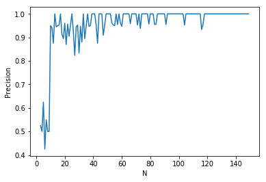
Figure 2: Precision of our test distinguishing uniform attachment from preferential as $n$ increases to $150$ (here, precision is the fraction of samples declared to be from preferential attachment, normalized by the number that, indeed, are). The fraction of trials in which preferential attachment was correctly identified (i.e., the recall) was always $1$. For each $n$, $40$ samples were taken, with each sample coming from uniform attachment with probability $1/2$.

Appendix A Proofs

In this section we prove Theorem 3.7 and Theorem 3.8.

A roadmap of the proof of Theorem 3.7 is as follows: we show that, regardless of which of $M_{0}$ or $M_{1}$ generated the observed trajectory, the test statistic $S$ is well-concentrated around its mean (in both cases, this is typically $\Theta(n)$). Furthermore, the hypothesis (23) allows us to conclude that $\mathbb{E}_{M_{0}}[S]$ and $\mathbb{E}_{M_{1}}[S]$ are well-separated. Thus, we are able to find an appropriate decision boundary for our test. The concentration of the test statistic boils down to concentration of each of its terms, which we are able to establish by rewriting them as an appropriate double integral in terms of a counting function ($N_{t}(p,q)$ below) which is analogous to the degree sequence in preferential attachment. We are then able to adapt techniques used to establish concentration of the degree sequence to complete the proof. The case for general $m\geq 1$ (where we recall that $m$ is an upper bound on the number of edges that may be added in a given timestep) is a corollary of the case for $m=1$, and so below we handle the case of $m=1$. This simplifies the notation somewhat: updates are now single vertices, and so we can use $p_{t,v}$ in place of $\pi_{t,v}$, etc.

A.1 Proof of Theorem 3.7

The analysis of the test boils down to showing concentration of the test statistic when the observed graph trajectory is from either $M_{0}$ or $M_{1}$. We will start by proving the following.

Proposition A.1 (Concentration of $d_{TV}(\hat{\mu}_{t},p_{t})$).

We have that for any models $M_{0},M_{1}$ as in the setting of Theorem 3.7, there is some $C>0$ such that for any sufficiently small $\epsilon_{1}>0$, there exists $\epsilon_{2}>0$ for which

$$\mathrm{Pr}_{M_{1}}[|d_{TV}(\hat{\mu}_{t},p^{M_{0}}_{t})-\mathbb{E}_{M_{1}}[d_{TV}(\hat{\mu}_{t},p^{M_{0}}_{t})]|>t^{-\epsilon_{1}}]\leq Ct^{-\epsilon_{2}}.$$ (25)

In order to show Proposition A.1, we rewrite the total variation distance as follows: in general, consider discrete random variables $X$ and $Y$. Then

$$d_{TV}(X,Y)=\frac{1}{2}\int_{0}^{1}\int_{0}^{1}N(p,q)|p-q|~{}dq~{}dp,$$ (26)

where $N(p,q)$ is the number of elements $x$ in the common domain of $X,Y$ for which $\mathrm{Pr}[X=x]=p$ and $\mathrm{Pr}[Y=x]=q$, and the integrals are with respect to discrete (Dirac) measures supported on the set of values for which $N(p,q)$ can possibly be nonzero. We see, then, that concentration of $d_{TV}(\hat{\mu}_{t},p^{M_{0}}_{t})$ will follow from concentration of $N_{t}(p,q)$ (now parameterized by $t$), where, in our case, the random variables in question are distributed according to $\hat{\mu}_{t}$ (which will correspond to the $p$ integrating variable) and $p^{M_{0}}_{t}=p_{t}$ (which will correspond to the $q$ integrating variable). More explicitly, $N_{t}(p,q)$ is the number of vertices $v$ in the interval $[t-1]$ whose empirical probability $\hat{\mu}_{t,v}$ is equal to $p$ and whose conditional probability at time $t$ according to model $M_{0}$ is equal to $q$. Note that $N_{t}(p,q)$ is a random variable, since it depends on $\hat{\mu}_{t}$, which itself depends on the observed trajectory. It is interesting to observe at this point that $N_{t}(p,q)$ is closely related, in the preferential attachment case, to the degree distribution, so ideas used in proving concentration of the degree sequence in that model can be generalized to prove concentration for $N_{t}(p,q)$. The next lemma gives the necessary concentration result.

Lemma A.2 (Concentration for $N_{t}(p,q)$).

Consider a model $M_{1}\in\mathcal{C}$. Then

$$\mathrm{Pr}_{M_{1}}[|N_{t}(p,q)-\mathbb{E}_{M_{1}}[N_{t}(p,q)]|\geq x]\leq 2\exp\left(-\frac{x^{2}}{c\cdot C(n)}\right),$$ (27)

for arbitrary $p,q\in[0,1]$, some positive constant $c$, and we recall that $C(n)=\Theta(n)$.

To prove this, we will use the method of bounded differences. Define the martingale $Z_{s}$, for $s\in\{t,t+1,...,t+C(n)\}$, as

$$Z_{s}=\mathbb{E}_{M_{1}}[N_{t}(p,q)|G_{s}].$$ (28)

The next lemma establishes the necessary bound on the martingale differences.

Lemma A.3 (Martingale difference bound).

Let $t\in[n]$, and consider the setting of Proposition A.1. Then for all $s\in[t+1,...,t+C(n)]$,

$$|Z_{s}-Z_{s-1}|\leq 2\Delta,$$ (29)

where $\Delta$ is the constant in the specification of $\mathcal{C}$ in Definition 3.2.

Proof A.4.

We consider the following pair of dynamic mechanisms: $M_{1}$ and $M_{1}^{\prime}$, which are coupled as follows: at times $1,...,s-1$, they are equal. At times $s$ and beyond, they evolve independently but according to $M_{1}$. We will show that we can rewrite the martingale differences in terms of $M_{1}$ and $M_{1}^{\prime}$ as follows:

$$Z_{s}-Z_{s-1}=\sum_{v=1}^{t}(\mathrm{Pr}_{M_{1}}[\hat{\mu}_{t,v}=p,p_{t,v}=q~{}|~{}G_{s}]-\mathrm{Pr}_{M_{1}^{\prime}}[\hat{\mu}_{t,v}=p,p_{t,v}=q~{}|~{}G_{s}]).$$ (30)

We will let $G_{s}$ be the graph at time $s$ according to $M_{1}$ and $G_{s}^{\prime}$ be the graph at time $s$ according to process $M_{1}^{\prime}$. To prove the identity, by linearity of expectation, we have

$$Z_{s}=\sum_{v=1}^{t}\mathrm{Pr}_{M_{1}}[\hat{\mu}_{t,v}=p,p_{t,v}=q~{}|~{}G_{s}].$$ (31)

An expression for $Z_{s-1}$ can similarly be written, with the only change being in the conditioning: $G_{s-1}$ instead of $G_{s}$. Now, conditioning on $G_{s}$ has the same effect on random variables from $M_{1}^{\prime}$ as conditioning on $G_{s-1}$, since the choices made by $M_{1}^{\prime}$ are independent of $G_{s},G_{s+1},...$. This gives us (30).

It remains to upper bound the right-hand side of (30). We note that

$$\mathrm{Pr}_{M_{1}^{\prime}}[\hat{\mu}_{t,v}=p,p_{t,v}=q~{}|~{}G_{s}]=\mathbb{E}_{M_{1}^{\prime}}[\mathrm{Pr}[\hat{\mu}_{t,v}=p,p_{t,v}=q~{}|~{}G_{s},G^{\prime}_{s}]].$$ (32)

I.e., we have conditioned on the choice at time $s$ according to $M_{1}^{\prime}$. We thus have

$$\mathrm{Pr}_{M_{1}}[\hat{\mu}_{t,v}=p,p_{t,v}=q~{}|~{}G_{s}]-\mathrm{Pr}_{M_{1}^{\prime}}[\hat{\mu}_{t,v}=p,p_{t,v}=q~{}|~{}G_{s}]$$ (33)

$$=\mathbb{E}_{M_{1}^{\prime}}[\mathrm{Pr}_{M_{1}}[\hat{\mu}_{t,v}=p,p_{t,v}=q~{}|~{}G_{s}]-\mathrm{Pr}_{M_{1}^{\prime}}[\hat{\mu}_{t,v}=p,p_{t,v}=q~{}|~{}G_{s},G_{s}^{\prime}]].$$ (34)

The quantity inside the expectation measures the difference in probabilities after the choice at time $s$ is made according to each mechanism. Using the conditional independence properties of the model class, at most $2\Delta$ vertices $v$ are such that this difference is nonzero. More precisely, let $W,W^{\prime}$ be the sets of vertices $v$ in the two respective trajectories such that $Y_{s,v}\neq Y_{s-1,v}$. Since all future vertex choices relating to vertices not in these sets are conditionally independent of them given $G_{s},G_{s}^{\prime}$, the above difference is only nonzero for vertices in $W$ and $W^{\prime}$. By the model assumptions, their cardinalities are both at most $\Delta$. This completes the proof.

With Lemma A.3 in hand, we apply the Azuma-Hoeffding inequality to prove Lemma A.2. The probability upper bound in Lemma A.2 is given by

$$2\exp\left(-\frac{x^{2}}{\sum_{s=t+1}^{t+C(n)}(2\Delta)^{2}}\right)=2\exp\left(-\frac{x^{2}}{(2\Delta)^{2}C(n)}\right).$$

We are finally ready to prove Proposition A.1.

Proof A.5 (Proof of Proposition A.1).

We will bound the integral representation (26) of the total variation distance.

We will start by ruling out large values of $q$. In particular, set $q=\Omega(t^{\delta})$, where $\delta=\frac{-1-\gamma-\epsilon}{\gamma}$, for an arbitrarily small positive $\epsilon$. That is, we wish to upper bound the integral

$$\left|\int_{0}^{1}\int_{q_{0}}^{1}N_{t}(p,q)-\mathbb{E}_{M_{1}}[N_{t}(p,q)]~{}dq~{}dp\right|.$$ (35)

By (15), we have

$$\int_{q_{0}}^{1}\mathbb{E}_{M_{1}}[N_{t}(p,q)]~{}dq\leq\int_{q_{0}}^{1}\mathbb{E}_{M_{1}}[N_{M_{0},t}(q)]~{}dq=O((qt)^{1+\gamma}),$$ (36)

where we recall that $\gamma<-2$. Similarly, by Markov’s inequality, we have that for any $x>0$,

$$\mathrm{Pr}[\int_{q=q_{0}}^{1}N_{t}(p,q)~{}dq>x]\leq\mathrm{Pr}[\int_{q=q_{0}}^{1}N_{M_{0},t}(q)~{}dq>x]\leq\frac{\int_{q=q_{0}}^{1}\mathbb{E}_{M_{1}}[N_{M_{0},t}(q)]~{}dq}{x}\leq\frac{O((qt)^{1+\gamma})}{x}.$$ (37)

In particular, we will choose $x=\Theta((qt)^{1+\gamma+\epsilon})$, which has the following consequence:

$$\mathrm{Pr}[\int_{q=q_{0}}^{1}N_{t}(p,q)~{}dq>x]=O((qt)^{-\epsilon}),$$ (38)

and since $q=\Theta(t^{-\delta})$ with $\delta>-1$, this tends to $0$ polynomially fast in $t$. All of this has the consequence that

$$\mathrm{Pr}[|\int_{0}^{1}\int_{q_{0}}^{1}N_{t}(p,q)-\mathbb{E}_{M_{1}}[N_{t}(p,q)]~{}dq~{}dp|>(qt)^{1+\gamma+\epsilon}]\leq O((qt)^{-\epsilon}).$$ (39)

We can thus ignore the range where $q=\Omega(t^{\frac{-1-\gamma-\epsilon}{\gamma}})$ for arbitrary fixed positive $\epsilon$. Now we focus on the small $q$ range: $\delta\leq\frac{-1-\gamma-\epsilon}{\gamma}$.

We will split the integral as follows:

$$\int_{0}^{t^{\frac{-1-\gamma-\epsilon}{\gamma}}}\int_{0}^{1}|N_{t}(p,q)-\mathbb{E}_{M_{1}}[N_{t}(p,q)]||p-q|~{}dp~{}dq$$ (40)

$$=\int_{0}^{t^{\frac{-1-\gamma-\epsilon}{\gamma}}}\int_{0}^{p_{0}}|N_{t}(p,q)-\mathbb{E}_{M_{1}}[N_{t}(p,q)]||p-q|~{}dp~{}dq$$ (41)

$$~{}~{}~{}+\int_{0}^{t^{\frac{-1-\gamma-\epsilon}{\gamma}}}\int_{p_{0}}^{1}|N_{t}(p,q)-\mathbb{E}_{M_{1}}[N_{t}(p,q)]||p-q|~{}dp~{}dq,$$ (42)

where $p_{0}=(1+c)t^{\frac{-1-\gamma-\epsilon}{\gamma}}$, with $c$ some small positive constant. The first integral on the right-hand side can be handled by noticing that $|p-q|=O(t^{\frac{-1-\gamma-\epsilon}{\gamma}})$ throughout, and by Lemma A.2 (with $x=t^{1/2+\varepsilon_{1}}$), with probability exponentially close to $1$ (with respect to $t$), we have

$$|N_{t}(p,q)-\mathbb{E}_{M_{1}}[N_{t}(p,q)]|\leq O(t^{1/2+\epsilon_{1}}).$$ (43)

Thus, the entire first integral is $\leq O(t^{1/2+\epsilon_{1}-\frac{1+\gamma+\epsilon}{\gamma}})$, which tends to $0$ because $\gamma<-2$.

To handle the second integral (where $|p-q|$ may be $\Theta(1)$), we notice that $|p-q|\leq 1$, and then, with high probability (by Markov’s inequality), $|N_{t}(p,q)-\mathbb{E}_{M_{1}}[N_{t}(p,q)]|\leq\mathbb{E}_{M_{1}}[N_{t}(p,q)]t^{\epsilon_{2}}$. This last inequality can be seen more precisely as follows: since $N_{t}(p,q)$ is a cardinality, it is lower bounded by $0$. Thus, if $N_{t}(p,q)<\mathbb{E}_{M_{1}}[N_{t}(p,q)]$, the difference between the two must be at most $\mathbb{E}_{M_{1}}[N_{t}(p,q)]$, which is certainly less than $\mathbb{E}_{M_{1}}[N_{t}(p,q)]t^{\epsilon_{2}}$. On the other hand, we can see by Markov’s inequality that

$$\mathrm{Pr}[N_{t}(p,q)>\mathbb{E}_{M_{1}}[N_{t}(p,q)]t^{\epsilon_{2}}]\leq\frac{\mathbb{E}_{M_{1}}[N_{t}(p,q)]}{\mathbb{E}_{M_{1}}[N_{t}(p,q)]t^{\epsilon_{2}}}=t^{-\epsilon_{2}}.$$

We can further upper bound by $\mathbb{E}_{M_{1}}[N_{t}(p,q)]\leq\mathbb{E}_{M_{1}}[N_{\hat{\mu}_{t}}(p)]$ (where $N_{\hat{\mu}_{t}}(p)$ is the number of vertices having conditional probability $p$ according to the distribution $\hat{\mu}_{t}$), and since $p\geq p_{0}$, $\mathbb{E}_{M_{1}}[N_{\hat{\mu}_{t}}(p)]=O(t^{-\epsilon_{3}})$, which is a consequence of the model class definition. In particular, the expected number of vertices $v$ with $p^{M_{1}}_{t,v}=p$ is at most $Ct^{-\epsilon}$, because of (15) and the fact that $p\geq p_{0}$ (in exactly the same way that we concluded (36)). This can be used to show that $\mathbb{E}_{M_{1}}[N_{\hat{\mu}_{t}}(p)]=O(t^{-\epsilon_{3}})$, using a proof analogous to the one that upper bounds the maximum degree for preferential attachment graphs.

Then, we are left with the double integral

$$t^{-\epsilon_{3}+\epsilon_{2}}\cdot\int_{0}^{t^{\frac{-1-\gamma-\epsilon}{\gamma}}}\int_{0}^{1}1~{}dq~{}dp=O(t^{\frac{-1-\gamma-\epsilon}{\gamma}+\epsilon_{2}}).$$ (44)

Recalling that $\gamma<-2$, we can make the exponent negative by setting $\epsilon$ and $\epsilon_{2}$ to be small enough, so the right-hand side of the above expression tends to $0$. More precisely, since $\epsilon>0$, the exponent is at most $-\frac{1}{\gamma}-1+\epsilon_{2}$. Since $\gamma<-2$, we have $-\frac{1}{\gamma}<1/2$, so the exponent is less than $-1/2+\epsilon_{2}$. Thus, if we choose $\epsilon_{2}<1/2$, the resulting exponent is negative. This yields the claimed result.

Now, we use Proposition A.1 to complete the proof of Theorem 3.7. We shall show that the test statistic is well concentrated. In particular, we want to show the following.

Theorem A.6 (Concentration of the test statistic).

We have, for any models $M_{0},M_{1}\in\mathcal{C}$ (or $M_{0}$, $M_{1}$ as in Definition 3.6), and for any $b\in\{0,1\}$ and any small positive constant $c$, that

$$\mathrm{Pr}_{M_{b}}[|S_{M_{0}}-\mathbb{E}_{M_{b}}[S_{M_{0}}]|>cn]\leq O(n^{-\epsilon_{1}}),$$ (45)

for some $\epsilon_{1}$.

Proof A.7.

We note that the terms $S_{j}=d_{TV}(\hat{\mu}_{r_{j}},p_{r_{j}}^{M_{0}})$ of the sum defining $S$ may be heavily dependent, due to the fact that the sampling intervals are likely to overlap heavily. To circumvent this, define $X$ to be the number of probe points $r_{j}$ for which

$$|S_{j}-\mathbb{E}_{M_{b}}[S_{j}]|>c/2,$$ (46)

where we recall that $S_{j}$ is the term in the sum defining $S$ corresponding to the $j$th probe point. By Markov’s inequality, for arbitrarily small $\epsilon_{1}>0$,

$$\mathrm{Pr}[X>n^{1-\epsilon_{1}}]\leq\frac{\mathbb{E}[X]}{n^{1-\epsilon_{1}}}.$$ (47)

We can calculate $\mathbb{E}[X]$ using linearity of expectation, and we see from Proposition A.1 that each term decays at least polynomially fast in $n$ to $0$. We thus have

$$\mathrm{Pr}[X>n^{1-\epsilon_{1}}]\leq n^{-\epsilon_{2}},$$ (48)

for some small $\epsilon_{1},\epsilon_{2}>0$. Now, if $X\leq n^{1-\epsilon_{1}}$, then $|S-\mathbb{E}[S]|\leq O(n^{1-\epsilon_{1}})+cn/2(1-O(n^{-\epsilon_{1}}))$, which implies the desired result.

Now, to finish the analysis of the error of the test, consider first the case where the sample trajectory comes from $M_{0}$. Then with probability $1-O(n^{-\epsilon_{1}})$, we have that $|S-\mathbb{E}_{M_{0}}[S_{M_{0}}]|<cn$ for arbitrary fixed $c>0$, so that the test correctly outputs $0$.

When the sample trajectory comes from $M_{1}$, note that for any small enough constant $\epsilon_{3}>0$, there is some $\epsilon_{1}>0$ such that with probability $1-O(n^{-\epsilon_{1}})$, $|S-\mathbb{E}_{M_{1}}[S]|<\epsilon_{3}n$. Then, by the condition in the theorem,

$$|\mathbb{E}_{M_{1}}[S]-\mathbb{E}_{M_{0}}[S]|\geq d_{n}(M_{0},M_{1})-\mathbb{E}_{M_{0}}[S_{M_{0}}]-\mathbb{E}_{M_{1}}[S_{M_{1}}]\geq Dn,$$ (49)

where $D$ is the constant alluded to in the theorem statement. Then, by the reverse triangle inequality, $|S-\mathbb{E}_{M_{0}}[S]|\geq\left||\mathbb{E}_{M_{0}}[S]-\mathbb{E}_{M_{1}}[S]|-|\mathbb{E}_{M_{1}}[S]-\mathbb{E}_{M_{0}}[S]|\right|\geq Dn-\epsilon_{3}n$, and for small enough $\epsilon_{3}$, this is $\geq Dn/2$. Thus, $|S-\mathbb{E}_{M_{0}}[S]|>\alpha(n)$ with high probability.

Theorem 3.8 is an immediate invocation of Theorem A.6.

We note that the proof of concentration for $m\geq 1$ follows by generalizing Lemma A.2. In particular, this may be done by induction on $m$, where $m=1$ forms the base case. We introduce some convenient notation: let $N^{(j)}_{t}(p,q)$ denote the number of multisets $S$ of vertices from $[t-1]$ of cardinality at most $j$ whose empirical probability (according to the choices of the vertices in the interval $[t,t+C(n)]$) is $p$ and for which $\prod_{v\in S}\pi_{t,v}=q$ (where the product takes into account the number of times each $v$ occurs in $S$). In particular, $N^{(m)}_{t}(p,q)=N_{t}(p,q)$.

Now, we can write $N^{(m)}_{t}(p,q)$ by considering the conditional probability assigned to the first vertex chosen in teach timestep:

$$N^{(m)}_{t}(p,q)=\int_{p^{\prime}\geq p}\int_{q^{\prime}\geq q}N^{(1)}_{t}(p^{\prime},q^{\prime})N^{(m-1)}_{t}(p/p^{\prime},q/q^{\prime})~{}dp^{\prime}~{}dq^{\prime}.$$ (50)

As above, we may neglect all but small values of $p^{\prime}$ and $q^{\prime}$ (on the order of $O(1/\sqrt{t})$), and the concentration of the remaining integral follows by induction.

References

- [Albert and Barabási(2002)] Réka Albert and Albert-László Barabási. Statistical mechanics of complex networks. Rev. Mod. Phys., 74:47–97, Jan 2002. 10.1103/RevModPhys.74.47. URL https://link.aps.org/doi/10.1103/RevModPhys.74.47.
- [Avin et al.(2008)Avin, Koucký, and Lotker] Chen Avin, Michal Koucký, and Zvi Lotker. How to explore a fast-changing world (cover time of a simple random walk on evolving graphs). In Automata, Languages and Programming, pages 121–132, Berlin, Heidelberg, 2008. Springer Berlin Heidelberg. ISBN 978-3-540-70575-8.
- [Baum and Petrie(1966)] Leonard E. Baum and Ted Petrie. Statistical inference for probabilistic functions of finite state markov chains. Ann. Math. Statist., 37(6):1554–1563, 12 1966. 10.1214/aoms/1177699147. URL https://doi.org/10.1214/aoms/1177699147.
- [Bollobás et al.(2001)Bollobás, Riordan, Spencer, and Tusnády] Béla Bollobás, Oliver Riordan, Joel Spencer, and Gábor Tusnády. The degree sequence of a scale-free random graph process. Random Structures & Algorithms, 18(3):279–290, 2001. 10.1002/rsa.1009. URL https://onlinelibrary.wiley.com/doi/abs/10.1002/rsa.1009.
- [Borgs et al.(2017)Borgs, Chayes, Cohn, and Veitch] Christian Borgs, Jennifer T. Chayes, Henry Cohn, and Victor Veitch. Sampling perspectives on sparse exchangeable graphs. arXiv e-prints, art. arXiv:1708.03237, Aug 2017.
- [Cherapanamjeri and Bartlett(2019)] Yeshwanth Cherapanamjeri and Peter L. Bartlett. Testing symmetric markov chains without hitting. In COLT, 2019.
- [Cover and Thomas(2006)] Thomas M. Cover and Joy A. Thomas. Elements of Information Theory (Wiley Series in Telecommunications and Signal Processing). Wiley-Interscience, New York, NY, USA, 2006. ISBN 0471241954.
- [Daskalakis et al.(2018)Daskalakis, Dikkala, and Gravin] Constantinos Daskalakis, Nishanth Dikkala, and Nick Gravin. Testing symmetric markov chains from a single trajectory. In Proceedings of the 31st Conference On Learning Theory, volume 75 of Proceedings of Machine Learning Research, pages 385–409. PMLR, 06–09 Jul 2018. URL http://proceedings.mlr.press/v75/daskalakis18a.html.
- [Diakonikolas et al.(2017)Diakonikolas, Gouleakis, Peebles, and Price] Ilias Diakonikolas, Themis Gouleakis, John Peebles, and Eric Price. Sample-optimal identity testing with high probability. Electronic Colloquium on Computational Complexity (ECCC), 24:133, 2017.
- [Ghoshdastidar et al.(2017)Ghoshdastidar, Gutzeit, Carpentier, and von Luxburg] D. Ghoshdastidar, M. Gutzeit, A. Carpentier, and U. von Luxburg. Two-sample hypothesis testing for inhomogeneous random graphs. preprint, 2017. arXiv preprint (arXiv:1707.00833).
- [Hofstad(2016)] Remco van der Hofstad. Random Graphs and Complex Networks, volume 1 of Cambridge Series in Statistical and Probabilistic Mathematics. Cambridge University Press, 2016. 10.1017/9781316779422.
- [Jeong et al.(2003)Jeong, Néda, and Barabási] H. Jeong, Z. Néda, and A. L. Barabási. Measuring preferential attachment in evolving networks. EPL (Europhysics Letters), 61(4):567, 2003. URL http://stacks.iop.org/0295-5075/61/i=4/a=567.
- [Nakagawa and Kanaya(1993)] Kenji Nakagawa and Fumio Kanaya. On the converse theorem in statistical hypothesis testing for markov chains. IEEE Trans. Information Theory, 39:629–633, 1993.
- [Natarajan(1985)] S. Natarajan. Large deviations, hypotheses testing, and source coding for finite markov chains. IEEE Transactions on Information Theory, 31(3):360–365, May 1985. ISSN 0018-9448. 10.1109/TIT.1985.1057036.
- [Newman(2010)] Mark Newman. Networks: An Introduction. Oxford University Press, Inc., New York, NY, USA, 2010. ISBN 0199206651, 9780199206650.
- [Orbanz and Roy(2013)] Peter Orbanz and Daniel Roy. Bayesian models of graphs, arrays and other exchangeable random structures. IEEE Transactions on Pattern Analysis and Machine Intelligence, 37, 12 2013. 10.1109/TPAMI.2014.2334607.
- [Ryabko(2017)] Daniil Ryabko. Hypotheses testing on infinite random graphs. In ALT, 2017.
- [Sreedharan et al.(2019)Sreedharan, Magner, Szpankowski, and Grama] J.K. Sreedharan, A. Magner, W. Szpankowski, and A. Grama. Inferring temporal information from a snapshot of a dynamic network. Nature Scientific Reports, 9:3057, 2019.
- [Veitch and Roy(2016)] Victor Veitch and Daniel M. Roy. Sampling and estimation for (sparse) exchangeable graphs. ArXiv, abs/1611.00843, 2016.
- [Wasserman(2010)] Larry Wasserman. All of Statistics: A Concise Course in Statistical Inference. Springer Publishing Company, Incorporated, 2010. ISBN 1441923225, 9781441923226.
- [Wolfer and Kontorovich(2019)] Geoffrey Wolfer and Aryeh Kontorovich. Minimax testing of identity to a reference ergodic markov chain. ArXiv, abs/1902.00080, 2019.