Constriction Percolation Model for Coupled Diffusion-Reaction Corrosion of Zirconium in PWR

Abstract

Percolation phenomena are pervasive in nature, ranging from capillary flow, crack propagation, ionic transport, fluid permeation, etc. Modeling percolation in highly-branched media requires the use of numerical solutions, as problems can quickly become intractable due to the number of pathways available. This becomes even more challenging in dynamic scenarios where the generation of pathways can quickly become a combinatorial problem. In this work, we develop a new constriction percolation paradigm, using cellular automata to predict the transport of oxygen through a stochastically cracked Zr oxide layer within a coupled diffusion-reaction framework. We simulate such branching trees by generating a series porosity-controlled media. Additionally, we develop an analytical criterion based on compressive yielding for bridging the transition state in corrosion regime, where the percolation threshold has been achieved. Our model extends Dijkstra’s shortest path method to constriction pathways and predicts the arrival rate of oxygen ions at the oxide interface. This is a critical parameter to predict oxide growth in the so-called post-transition regime, when bulk diffusion is no longer the rate-limiting phenomenon.

Keywords: percolation, corrosion cracking, zirconium oxidation.

$*$California Institute of Technology, 1200 E California Blvd, Pasadena, CA 91125

$\dagger$University of California, 410 Westwood Plaza, Los Angeles, CA 90095

$\ddagger$Bahçeşehir University, 4 Çırağan Cad, Beşiktaş, Istanbul, Turkey 34349

1 Introduction

The corrosion and fracture of zirconium clad in the presence of high-temperature water is the main failure mechanism in cooling pipelines of pressurized water reactors (PWR). [1, 2, 3, 4] The gradual oxidation is the result of diffusion of oxygen into the depth of metal matrix, followed by chemical reaction in the corrosion front. Several studies have shown that the oxide scale grows as cubic law versus time during pre-transition period ( $\sim t^{\nicefrac{{1}}{{3}}}$) as opposed to typical parabolic diffusion behavior ($\sim t^{\nicefrac{{1}}{{2}}}$). [5, 6, 7] The oxygen diffusion into metallic structure leads to large augmentation in volume and internal compressive stresses due to Pilling-Bedworth ratio. [8] The fracture reason is attributed to the residual stresses from cyclic cooling, embrittlement from hydrides precipitation and phase transformation during non-stoichiometric oxidation of zirconium as well as yielding due to compressive and the balancing tensile stresses.[9, 10, 2]. The randomly-distributed cracks are merely sensitive to original spatial distribution/concentration of defects/grain boundaries [11, 12]. Consequently water can penetrate into the cracks and the oxygen gets easy access to corrosion sites without the original pre-cracking diffusion barrier. This event leads to jump in corrosion kinetics [7]. The diffusion process via grain boundaries and material matrix (i.e lattice) has been studied in the context of percolation [13]. One of the illustrative methods for percolation is cellular automata paradigm which is typically studied in the two distinct context of site and bond percolation. [14, 15, 16] Later studies have complemented the percolation with reaction in the diffusion front. [17] However, the precise quantification of diffusion through the shortest constriction pathways, particularly during the oxidation process and wide range of percolation regime, distinguished by fracture has not been addressed before. In this paper, we develop a coupled diffusion-reaction framework, based on the two percolation paradigms for predicting the corrosion rates after initiation of cracks. The constriction and tortuous geometry of percolation pathways as well as the reactive term has central role in our model for predicting the ultimate corrosion kinetics.

2 Methodology

2.1 Approach

The inhomogeneous percolation of the oxygen within the oxide scale could either be interpreted as diffusion within the cracked network during post-transition regime or within the grain boundaries or material imperfections during the pre-transition development. In fact such two patterns are highly correlated as the cracking is the most feasible to occur through relatively weaker grain boundaries/imperfections. During the initial stage of oxidation, the abundant oxygen from electrolyzed water reacts with the zirconium metal and therefore the corrosion is in fact reaction-limited. However, after a sufficient penetration of oxide scale into the depth, the reaction front suffers from “breathing” and corrosion kinetics turns to be dominantly diffusion-limited. Upon the fracture, the cracks propagate in columnar shape, preferably along the weakest shear bands (i.e. grain boundaries) and the water gets easy access to the oxidation front (i.e. oxide/metal interface).

Figure 1: Schematics of cracks network (left) and their corresponding constriction rivers (right).

2.2 Percolation clusters

2.2.1 Characterization

Given a general network of cracks in Figure 1, for the purpose of simulation we can differentiate each one either via the connection to the either of the interfaces, the constriction value with the inherent tortuosity as below:

0. Islands: These confined areas have no access to the any of the interfaces. Therefore their role can be neglected.

1. Partial Cracks: These cracks need have partial progress within the oxide layer from the water/oxide interface. The transport of water occurs through the tortuous crack, while the rest of the diffusion within the oxide occurs through the shortest path. (i.e. straight line.)

2. Full cracks: These cracks provide full connection between the water/oxide and oxide/metal interfaces.

The tortuous geometry of each crack not only elongates the transport route, but also provides a projection for the transport flux. Therefore the diffusion coefficient for each crack $D_{cr}$is expressed as:

$$\frac{\tau_{cr}^{2}}{D_{cr}}=\frac{\tau_{ox}^{2}}{D_{ox}}+\frac{\tau_{w}^{2}}{D_{w}}$$ (1)

where $D$ and $\tau$are the diffusion coefficient and tortuosity of crack, oxide and water respectively. Comparison the diffusivity values for oxide scale $D_{ox}\approx 10^{-17}m^{2}/s$ [18] and water $D_{w}\approx 10^{-8}m^{2}/s$ [19] leads to:

$$D_{ox}<D_{part}\ll D_{full}<D_{w}$$ (2)

where $D_{part}$ and $D_{full}$ are the diffusion coefficient values for the partial and full cracks.

The significant difference in Equation 2 addresses that there is a jump in the oxide growth rate when the porosity of crack network reaches the percolation threshold value $p=p_{c}$. Consequently, the homogenized diffusivity $D_{EFF}$ during post-transition period can be simplified in $2D$ as:

$$D_{EFF}\approx\frac{D_{w}}{L}\sum_{k=1}^{n}\frac{l_{k}}{\tau_{k}^{2}}$$ (3)

(a) PseudoFlowchart for cracks.

(b) Crack density.

Figure 2: Computational development chart (left) and crack density (right).

We simulate such medium by generating stochastic binary medium with the developing porosity in time. Utilizing the cellular automaton paradigm, we extend Dijkstra’s shortest path algorithm [20], for extracting the Constriction rivers (CRs). The diffusion through cracks has been simulated by the square bond percolation ($4^{2}$), accompanied with the site percolation method for comparison and verification. The percolation threshold probability $p_{c}$, which divides the pre and post-transition growth regimes, for the former is known to be $\approx 0.5$ while in the latter is $\approx 0.5928$, after which some of the partially-formed cracks tend full cracks. [21, 22, 23]

Figure 2a explains the computational algorithm for extracting the constriction pathways illustrated in Figure 1. We summarize the procedure as below:

i. Forward percolation: Starting from the water/oxide interface ($y=0$), percolate forward from the $1^{st}$ order neighbors and index each new addition in descending order. Such index tangibly correlates with the amount of time the water has reached that location. For full cracks, the percolation will reach to the oxide/metal interface ($y=s$).

ii. Backward Percolation: The largest index in the oxide/metal interface ($y=s$) indicates that water has reached there the earliest. Therefore, starting from that element, we revert backwards from the $1^{st}$ order neighbors by ascending order of indexes until reaching back the water/metal interface ($y=0$). The extracted path is the shortest distance between two interfaces. The usability of pores within the cracked medium depends on if they have been captured as a part of the shortest path. For the pathways of the same beginning/end (i.e. same length) one of them is eliminated in favor of the other.

iii. Constriction Percolation: The constriction along each river would control the diffusion and the flux of water. In order to capture that, we periodically increase the thickness ($Dim$) in 2D (i.e. cube in 3D) in cellular automata paradigm. Additionally starting from shortest river, obtained in the first two steps ensures the shortest path for the thickest possible river as well.

Figure 2b illustrates the density of states ($M$) for the obtained partial and full cracks based on original porosity and Figure 3a is a sample illustration based on square site percolation ($4^{2}$) beyond percolation limit. ($p>p_{c}$). The black routes are the only top-to-bottom connection pathways and the color map value on each site correlates with the time oxygen has reached that location. We will elaborate on this further in

(a) A site percolation sample. $p=0.55$.

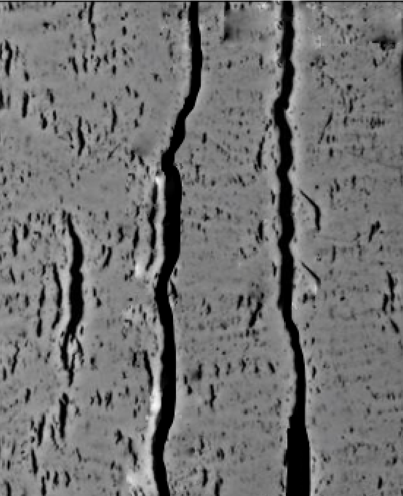
(b) Original image.

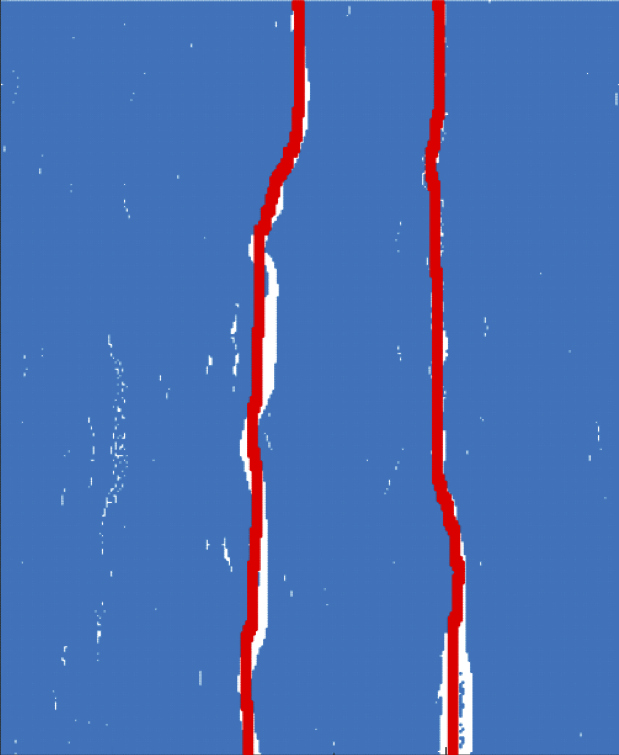
(c) Illustration of $CRs$ (in red).

Figure 3: (a) Sample site percolation: blue: cracked network, green: partial cracks, red: full cracks. (b) Original cracked oxide image. (c) Extracted constriction rivers (blue: metal, white: voids, red: CRs).

The extraction of CRs from the given cracked medium would be possible by implementing binarizaion on the original grayscale image (Figure 3b) via Otsu’s method [24]. This could be possible choosing a threshold such to minimize the intra-class variance $\sigma^{2}$ defined as below:

minimize $\sigma^{2}$ such that:

$$\text{}\begin{cases}\sigma^{2}=\omega_{1}\sigma_{0}^{2}+\omega_{2}\sigma_{1}^{2}\\ \omega_{1}+\omega_{2}=1\end{cases}$$ (4)

where $\sigma_{0}^{2}$ and $\sigma_{1}^{2}$ are the variance for the divided black and white groups and $\omega_{1}$ and $\omega_{2}$ are their corresponding fraction. Performing the procedure in flowchart 2a on the original image (Figure 3b), the $CRs$ could be obtained as shown in Figure 3c The real-time simulation of extracting of constriction percolation pathways is shown in the supplemental materials.

Furthermore the tortuosity of cracked pathways can be calculated from the extracted $CRs$, the average tortuosity $\bar{\tau}$ for site and bond percolations are shown versus original porosity in 2 and 3 dimensions in Figure 4a. The computed diffusion coefficients from Equation 3 is shown in Figure 4b respectively for partial ($p<p_{c}$ ) and full ($p>p_{c}$) cracks.

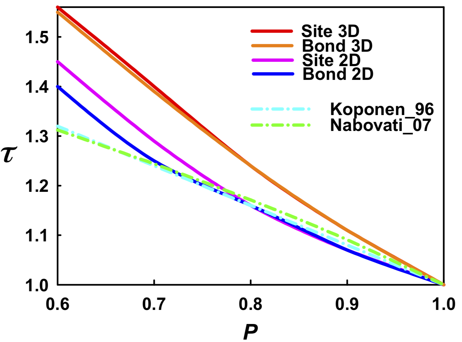
(a) Tortuosity.

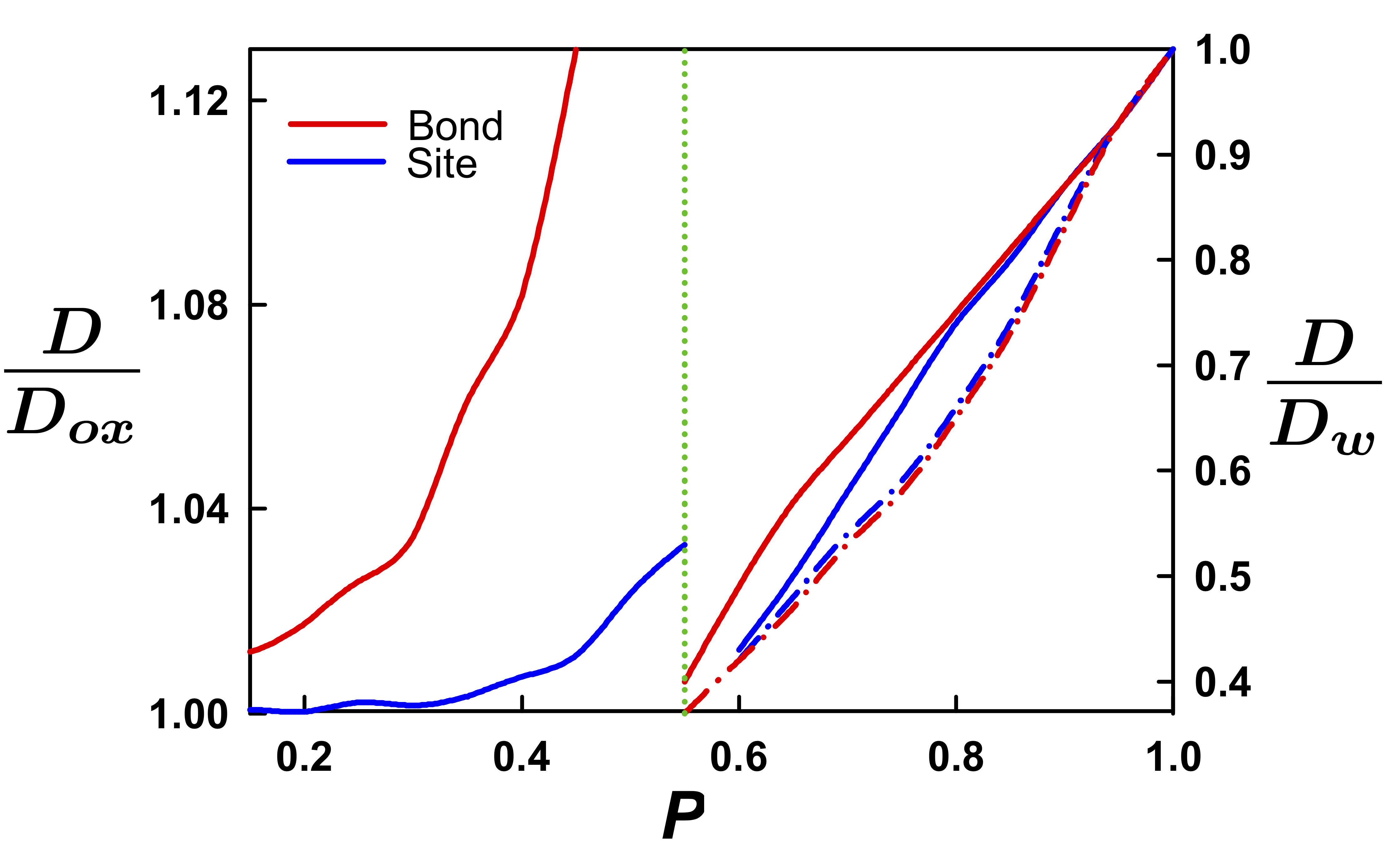
(b) Diffusion coefficient.

Figure 4: The geometric role of cracks on the diffusivity.

2.2.2 Scaling Dimension

Scaling dimension $\alpha$, in fact represent the scaling role of the percolating cluster versus the dimension of the medium. In other words, for the percolation paradigm with the domain scale $L$, there is a power coefficient $\alpha\in{\rm R}$ for which the density of states for percolating cluster $M(L)$ correlates with the domain scale as:

$$M(L)\propto L^{\alpha}$$ (5)

We have performed the constriction percolation paradigm in square bond paradigm ($4^{2}$), given in flowchart 2a from the center of the medium, for various scales. Upon reaching the threshold (i.e. two facing boundaries) the computations has been stopped. The density of states for the connecting percolation pathways $M(L)$ has been plotted against the domains scale $L$in Figure 5a, versus the exponent limits given in the literature. [21]. To ensure the statistical converges, each simulation point is the average of 10 stochastic computations. Additionally, Figure 5b visualizes a sample percolation computation for the domain scale of 500.

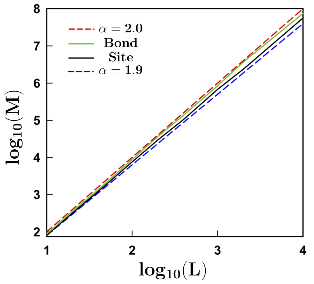
(a) Scale dependency of density of states (M) based on site and bond percolation.

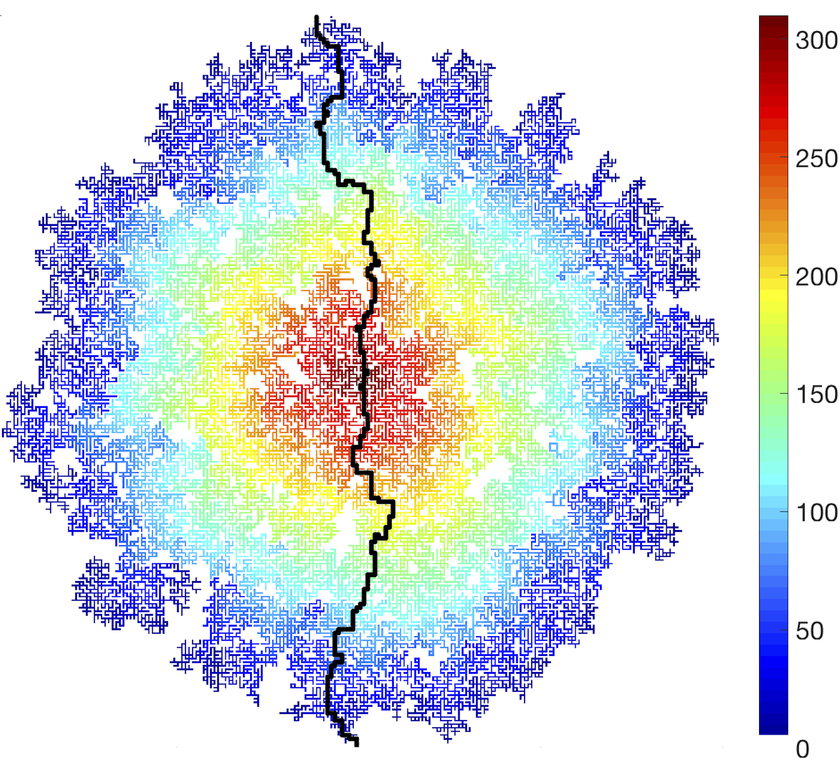
(b) A bond percolation from center. ($p=0.65$)

Figure 5: Scale studies.

2.3 Formulation

During the oxidation process, initially the oxygen from the water electrolysis starts filling in the zirconium matrix until reaching the stoichiometric limit, where the zirconium dioxide forms. Subsequently the oxide/metal (i.e. reaction site) growth deeper within the metal during so-called pre-transition regime. However, after growing to a sufficient extent, the fracture gradually occurs and the cracks accumulate and propagate up to the corrosion front. Therefore, the transport of oxygen dominantly occurs via water percolation within the crack network, leading to a sudden jump in corrosion kinetics.

Merging two growth regimes, the evolving oxygen concentration ($O$) is given via the extended diffusion Equation in $1D$ as[25]:

$$\frac{\partial O}{\partial t}=D(T)\left(\frac{\partial^{2}O}{\partial y^{2}}+\Delta(T)\frac{\partial O}{\partial y}\right)-kO$$ (6)

where $y$ is the depth variable and $t$ is the time defined in Figure 1. The extra term in the $RHS$ of Equation 6 represents the thermomigration. According to the Suret-ludwig effect, the vacancy mediated motion of substitutional atoms is expected to occur down the temperature gradient, while the interstitial solute move in the opposite direction. [26] The second extra term represents the consumption of oxygen due to oxidation process and $k$ is the reaction constant.

The diffusivity $D(T)$ is regime-dependent and defined as below:

$$D(T)=\begin{cases}{\displaystyle\Large D_{0,ox}\exp\left(\cfrac{-Q_{ox}}{RT}\right)}&\text{Pre}\\ {\displaystyle\Large D_{0.w}\left[\frac{T}{T_{s}}-1\right]^{\gamma}}&\text{Post}\end{cases}$$ (7)

where the first Equation shows the Arrhenius-type relationship [18] and the second Equation represents Speedy-Angell power law self-diffusion of water.[19]

Therefore the $\Delta(T)$ is obtained from chain derivation as:

$$\Delta(T)=\begin{cases}{\displaystyle\Large\frac{Q_{ox}}{RT^{2}}\frac{dT}{dy}}&\text{Pre}\\ {\displaystyle\Large\frac{\gamma}{T-T_{s}}\frac{dT}{dy}}&\text{Post}\end{cases}$$ (8)

There is presumably no oxygen in the zirconium matrix at the beginning, therefore the initial condition would be:

$$O(y,0)=0$$ (9)

On the other hand, on the water/oxide interface there is constant concentration of oxygen provided from water radiolysis ( $O_{0}$) :

$$O(y,0)=O_{0}$$ (10)

$O_{0}$ has been considered as the molar value of oxygen in the water. (Table 1).

and no oxygen can escape from clad into the fuel side: (i.e. $J_{O}(L,t)=0$) [27]

$$\frac{\partial O}{\partial y}(L,t)=0$$ (11)

Generally during the diffusion, the oxygen should migrates inside the zirconium matrix, however as the reaction occurs much faster rate than the diffusion ($k\gg D$), the entire diffused oxygen reacts towards the formation of oxide scale upon reaching the reaction sites (i.e. diffusion front). Therefore the effective depth of the oxide layer at a given time could be obtained by leveling the entire diffused oxygen it with the stoichiometric saturation value of zirconium metal to oxide as:

$$s(t)=\frac{1}{2Z_{0}}\int_{0}^{t}O(y,t)dy$$ (12)

The coefficient of 2 is due to stoichiometric ratio of oxygen to zirconium (i.e. $\nicefrac{{N_{O}}}{{N_{Zr}}}=2$).

2.3.1 Transition state:

The fracture in the zirconium oxide, is attributed to few factors, such as the residual stresses during heating/cooling cycles and the compressive stresses mainly via shear bands [7, 28]. Here, we develop a simple formulation based on the latter to describe the onset of cracking throughout oxidation development. The treat the oxide scale as an epitaxial layer on the substrate metal surface, exposed to biaxial stresses. Assuming the original cross sectional area of zirconium metal $A_{0}$ and oxide depth $L$ , the corresponding oxide volume would be $V=AL$ . Adding the increment of $ds$ to the oxide depth would lead to increment of volume as $dV=Ady+ydA$ . Due to confined boundaries from lateral dimensions we have $ydA\approx 0$, and therefore the growth can be approximated as 1D.

Having one dimensional growth, the addition of the infinitesimal depth $ds$ into the oxide layer would increase the total depth by $R_{PB}dy$ . ($ds=R_{PB}dy)$ and reduce the zirconium depth by $dy$. The variation in total thickness $(dy)_{tot}$ consequently is:

$$(dy)_{tot}=(dy)_{ox}-(dy)_{zr}=ds-\cfrac{ds}{R_{PB}}=(\cfrac{R_{PB}-1}{R_{PB}})ds$$

The relative volume variation becomes:

$$\cfrac{dV}{V}=\cfrac{dy}{y}=\cfrac{(R_{PB}-1)ds}{R_{PB}L+(R_{PB}-1)s(t)}$$

where ($R_{PB}-1$) could also be tangibly interpreted as the addition coefficient in $1D$. Subsequently, for the biaxial loading, the compressive stress is twice the homogeneous pressure $\sigma=2P$. Thus the homogeneous stress within the oxide scale could be predicted from real-time computation as:

$$\sigma(t)=2K(R_{PB}-1)\int_{0}^{s(t)}\frac{d\omega}{R_{PB}L+(R_{PB}-1)\omega(t)}$$ (13)

where $K$ is the bulk modulus. On the verge of fracture, the stress reaches the compressive yield limit in the oxide medium. Upon reaching the transition moment we have: $\sigma(t)=S_{yc}$ and $s=s_{c}$. Therefore, solving the Equation 13 analytically leads to:

$$s_{c}=\frac{R_{PB}L}{R_{PB}-1}\left(\exp\left(\frac{S_{yc}}{2K}\right)-1\right)$$ (14)

The range values from table 1 for compressive yield stress and the bulk modulus for zirconium oxide are $S_{yc}\in[1.2-5.2]GPa$ and $K\in[72-212]GPa$, therefore the transition range of oxide scale would be:

$$s_{c}\in[0.4-5.1]\mu m$$ (15)

The simulation parameters for oxide scale growth are shown in Table 1.^,

Parameter	Value	Unit	Ref.
$D_{0,w}$	$1.6\times 10^{-8}$	$m^{2}/s$	[19]
$T_{s}$	$215$	$K$	[19]
$\gamma$	$2.1$	$[]$	[19]
$D_{o.ox}$	$10^{-10}$	$m^{2}/s$	[18]
$Q_{ox}$	$52$	$kcal/mol$	[18]
$S_{yc}$	$[1.2-5.2]$	$GPa$	azom
$K$	$[72-212]$	$GPa$	azom
$T_{0}$	$600$	$K$	[27]
$T_{L}$	$660$	$K$	[27]
$L$	$50$	$\mu m$	[27]
$O_{0}$	$62.5$	$M$	[30]
$Z_{0}$	$71$	$M$	[31]
$k$	$7.1\times 10^{-6}$	$s^{-1}$	[29]

Table 1: Simulation parameters.

Using the Equation 6 with the transition scale predicted in Equation 14 and the parameters given in Table 1, the real-time stress development in the oxide scale is computed in Figure 6a in versus the porosity values from partial cracks. From the Equation 6 and the corresponding oxide scale thickness Equation 12, the post transition growth rates has been illustrated in Figure 6c in higher porosities values. The coupled growth regimes, are illustrated Figure 6b with the corresponding sensitivity analysis for post transition regime.

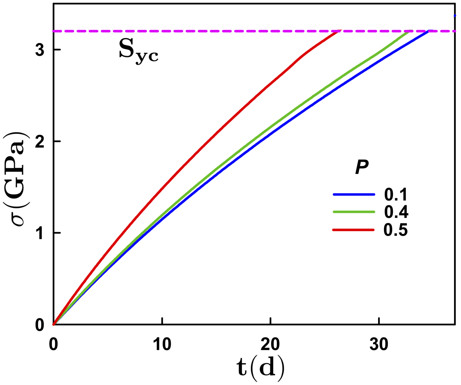
(a) Stress development.

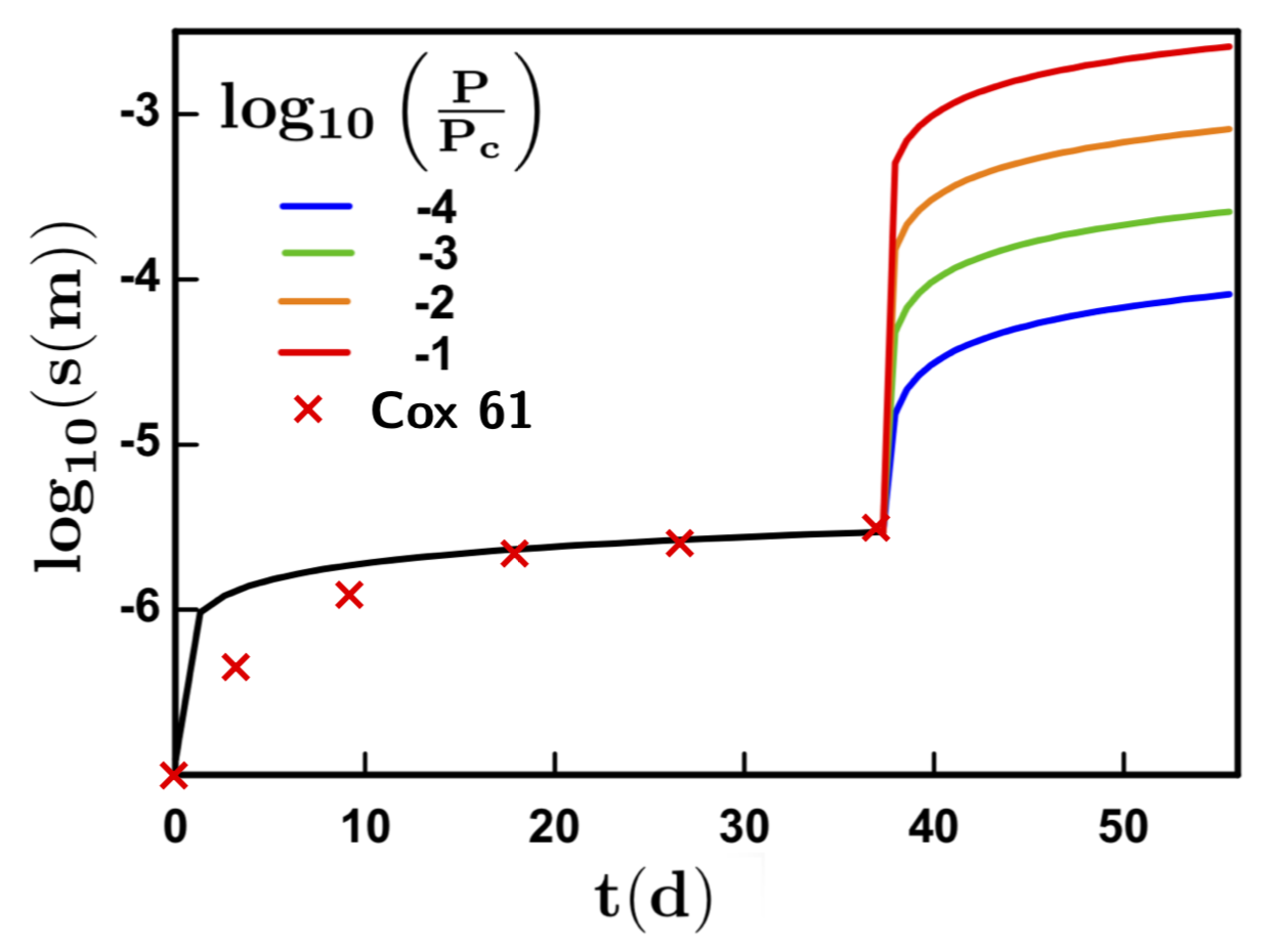
(b) Sensitivity analysis. ($b_{pre}=0.36$ )

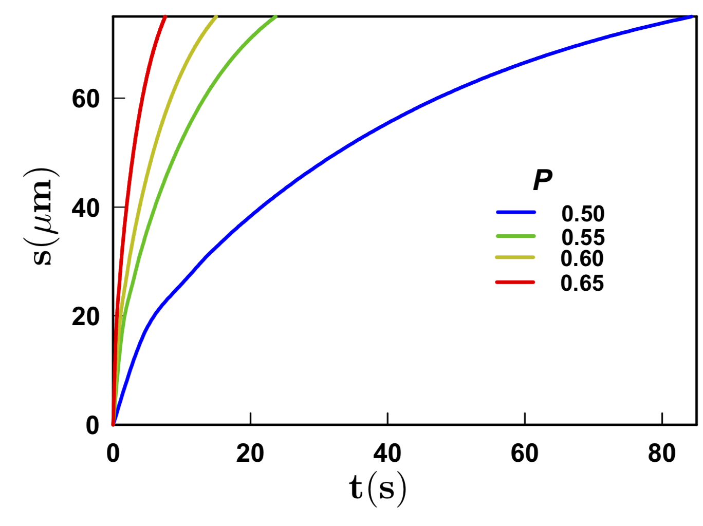
(c) Post-transition. ($b_{post}\approx 0.34)$

Figure 6: (a) Pre-transition growth regime. (b) Sensitivity analysis growth regime during the post-transition regime. (c) Growth regime after the fracture for difference porosity values.

2.3.2 Temperature profile:

As the diffusivity values are very sensitive to the temperature, consideration of it’s distribution would be very useful realization. Comparing the diffusivity of oxygen in zirconium ($D_{ox}\approx 10^{-15}m^{2}/s$) with thermal diffusivity of Zirconium ($\alpha\approx 10^{-8}m^{2}/s$), one ascribes:

$$\frac{\partial T}{\partial t}\gg\frac{\partial O}{\partial t}$$

which implies that the kinetics of thermal propagation is significantly higher and therefore at any infinitesimal period of time, temperature profile has already reached the steady-state regime.(i.e. $T(y,t)\approx T(y)$ ) As the oxide layer grows, it makes a relative insulation between two ends, and consequently the heat flux ($q$) decreases, until fracture. The enthalpy of the oxidation is negligible relatively to the amount of transferred heat ($\Delta H_{rxn}\ll q$), therefore the heat flux is controlled by the insulation of oxide layer:

$$q(t)=-\kappa_{ox}\left(\frac{dT}{dy}\right)_{ox}=-\kappa_{Zr}\left(\frac{dT}{dy}\right)_{Zr}\leq-\kappa_{Zr}\frac{T_{L}-T_{0}}{L}$$ (16)

The temperature at the oxide/metal interface ($T_{s}$) correlates directly with their thermal conductivity and is inversely proportional with the distance from each boundaries. Therefore if we define the conductivity coefficient ($\beta:=\kappa/l$) . Therefore the interface temperature ($T_{s}$) could be linearly obtained as:

$$T_{s}=\left(\frac{\beta_{ox}}{\beta_{ox}+\beta_{Zr}}\right)T_{0}+\left(\frac{\beta_{Zr}}{\beta_{ox}+\beta_{Zr}}\right)T_{L}$$ (17)

where $\beta_{Zr}=\kappa_{Zr}/(L-s(t))$ and $\beta_{ox}=\kappa_{ox}/s(t)$ respectively.

2.3.3 Numerical stability:

We utilize the finite difference scheme to solve the PDE Equation 6 in space and time. If ($O_{i}^{j}$) represents the oxygen concentration at depth ($y_{i}$) and time ($t^{j}$), adopting forward difference method in time and space ($FTFS$), we get:

$$O_{i}^{j+1}=(1-2Q_{1}-Q_{2}-Q_{3})O_{i}^{j}+(Q_{1}+Q_{2})O_{i+1}^{j}+Q_{1}O_{i-1}^{j}$$ (18)

where $Q_{1},$$Q_{2}$ and $Q_{3}$ are the quotients defines as below:

$$Q_{1}=\frac{D\delta t}{\delta y}$$ (19)

$$Q_{2}=\begin{cases}\displaystyle{\Huge\frac{D\delta t}{\delta y}\frac{Q_{ox}}{RT^{2}}\frac{dT}{dy}}&\text{Pre}\\ \displaystyle{\Huge\frac{D_{0}\gamma\delta t}{\delta y}\left[\frac{T}{T_{0}}-1\right]^{\gamma-1}\frac{dT}{dy}}&\text{Post}\end{cases}$$ (20)

and

$$Q_{3}=k\delta t$$ (21)

where $\delta t$ and $\delta y$ are the segmentations in time and space. To ensure the stability, we must have:

$$1-2Q_{1}-Q_{2}-Q_{3}\geq 0$$

Therefore, to satisfy the criteria for both growth regimes, the following condition would suffice:

$$\delta t:\leq\frac{\delta y^{2}}{2D}$$ (22)

3 Results and Discussions

The computational results demonstrate the cooperative role of diffusion and migration for corrosion rate as well as significant sensitivity of corrosion rate for the porosity values beyond percolation threshold. Following the computational algorithm in flowchart 2a the percolation pathways could be obtained through the crack network. The density of states $M$ for partial and fully-connecting cracks is shown in Figure 2b. It is obvious that upon increasing the porosity $p$, the percolation through the partial cracks augments earlier than the full cracks. Such a contrast also has been visualized in the Figure 3a, where the spectrum of colors represent the amount of time the oxygen has been present in those sites. Albeit possessing less density of states, the full cracks have significantly more impact on the oxide growth rate, merely due to much higher value of water self-diffusion coefficient relative to the zirconium oxide.

The method can predict the rate of corrosion from experimental images by means of image processing. The bare image from cracked zirconium oxide in Figure 3b can be binarized via Otsu’s minimization of intraclass variance $\sigma^{2}$ in Equation 4. The extracted $CRs$ are shown in Figure 3c.

Performing scale studies, Figure 5a shows that the mean statistical density of states for the percolation samples, correlates with the power law growth regime $1.9<\alpha<2.0$ as a verification. [21] Additionally in this graph, the bond percolation curve stands higher than the site percolation. This comparison will be verified mathematically in Equation 23. Note that upon reaching the percolation threshold, the constriction river most likely is the thinnest on the verge of percolation threshold ($p\approx p_{c}$).

Given certain porosity value $p$, the water is transported through a torturous pathway from the water/metal interface to reach the oxidation front (i.e. oxide/metal interface). For lower values of porosity, merely close to the percolation threshold $p\approx p_{c}$, there will be a signifiant search for the shortest pathway due to scarcity of the penetrable areas and the tortuosity value of the shortest path will be the highest. As the porosity value increase, the possibility of more direct connection is also becomes greater and therefore the corresponding tortuosity value is reduced, such that in the limit of full porosity ($p\rightarrow 1$) the connection routes are almost straight and the tortuosity value merges to unity. This trend has been illustrated in Figure 4a and shows a nice agreement with previous findings. [32, 33] Additionally, in 2D percolation the transport is possible from 4 pathways, where in 3D the percolation can occur from 6 directions, where, in each case, only one direction is considered to be straight. Thus, the probability of twisted percolation in 2D would be $\nicefrac{{3}}{{4}}$, whereas in 3D it would become $\nicefrac{{5}}{{6}}$. This clearly shows that the 3D percolation would generate more tortuosity in average versus 2D percolation, as shown in Figure 4a.

The Diffusion coefficient values based on Equations 1 and 3 are illustrated in Figure 4b. Due to lower tortuosity values in 3D relative to 2D percolation (Figure 4a), it is obvious from Equation 1 that the diffusion coefficient also follows the same comparative trend. Additionally, the values for bond percolation is more than site percolation, hereby we prove that this is always true.

Given certain porosity $p$ , the bond percolation develops more diffusion coefficient versus site percolation. The underlying reason is that any square bond percolation paradigm ($4^{2}$), $p_{b}$ can be interpreted by an equivalent bond percolation scheme ($4^{2}$), $p_{eq,s}$ where each connection point (i.e. corner) could be treated as a site per see. Assuming the dimension in a 2D bond percolation to be $d$ and the number of available sites for percolation is $M$, the porosity will be calculated as:

$$p_{b}=\frac{M}{d^{2}}$$

where the dimension in the equivalent site percolation would be $2d+1$ , due to inclusion of connection points as available site.Therefore, the elements in equivalent site percolation paradigm would be $n+(d+1)^{2}$, and:

$$p_{eq,s}=\frac{M+(d+1)^{2}}{(2d+1)^{2}}$$

Hence, we need to prove the following inequality:

$$\frac{M+d^{2}+2d+1}{4d^{2}+4d+1}<\frac{M}{d^{2}}$$

performing rearrangements and since always $p_{b}<1$ , we have $M<d^{2}$ and we arrive at:

$$d^{4}+2d^{3}-3Md^{2}-4Md-M+d^{2} <$$

$$d^{4}+2d^{3}-3d^{4}-4d^{3}-d^{2}+d^{2}<0$$

Therefore we only need to prove the RHS inequality, which gets simplified into:

$$-2d^{2}(d+2)<0\text{ $\checkmark\ $}$$

since this equation is always true, we have:

$$p_{eq,s}>p_{b}$$ (23)

Thus, given a certain porosity, the bond percolation creates a larger cluster (i.e. available sites) versus the site percolation, which is obvious in Figure 4b.

For the transition regime based on compression stress, if the average values are considered for the range of compressive yield strength and th bulk modulus given in Table 1, the mean value for the critical thickness for the transition state from Equation 15 would be $s_{c}=2.75\mu m$ which is in nice agreement with the values given in current literature. [34, 2] Such transition state has been addressed with the close proximity in recent findings with an alternative method as well. [27]

The large amount of Pillar-Bedworth ratio $R_{PB}$ indicates upon formation and advancing oxide layer, the compressive stresses accumulate in real time. We have captured such stress augmentation in Figure 6a, versus the pre-transition porosity $p$ (i.e. partial cracks/ imperfections), until the yield limit (i.e. fracture). It is obvious that the higher density of imperfections will reduce the transition time. From Equation 13 the stress growth $\sigma(t)$ depends to the oxide scale $s(t)$. This correlation in particular is linear (i.e. direct) for higher values of original thickness, where denominator will remain relatively invariant, and therefore the cubic growth regime is expected (as will be explained next) for stress growth behavior, where $s\ll L$. Nevertheless, the real-time stress can be obtained from Equation 13 as:

$$\sigma(t)=2K\ln\left(\frac{R_{PB}-1}{R_{PB}}s(t)+1)\right)$$

which shows exponential decay behavior as illustrated in Figure 6a.

Figure 6b illustrates the all-in-one plot for oxide evolution. The breakaway point has been analytically calculated from Equation 15 and the sensitivity analysis has been performed for the post-transition regime based on the logarithmic distance from percolation threshold. The growth regime in either stage can be approximated with the power law growth in time as:

$$s(t):=at^{b}$$ (24)

Correlating the pre-transition growth regime with power law, the exponent value of $b_{Pre}=0.35$ is obtained, which is in very high agreement with the value of $b\approx\nicefrac{{1}}{{3}}$ in the literature. [35, 7, 27, 28] On order to verify the simulation results, we use corresponding experimental results from [7], where the the increase in the mass of oxide samples have been correlated with a cube of time and within 38 days of corrosion has possessed the weight addition of $18\nicefrac{{mg}}{{dm^{2}}}$ which translates to the oxide thickness value of $2.76\mu m$.

For fundamental understanding of cooperating role of diffusion, reaction and thermomigration terms, one can start from the typical diffusion Equation given as below:

$$\frac{\partial O}{\partial t}=\frac{\partial}{\partial y}\left(D\left(\frac{\partial O}{\partial y}\right)\right)$$ (25)

The typical solution for this Equation will have a parabolic trend. ($s\propto t^{\nicefrac{{1}}{{2}}}$). The subtraction of significant consumption term ($-kO$) with the presence of thermomigration term $D\alpha(T)\cfrac{\partial O}{\partial y}$ in Equation 6, would bend down (i.e. reduce) the oxide evolution curve, such that in our simulations it correlates with a lower power value. (i.e. $b\approx 0.36$). The aforementioned bending effect has been addressed by presence of exponentially reducing electric charge distribution and the corresponding electrostatic field at reaction sites during previous study.[27]

Additionally, Figure 6b addresses the extremely high sensitivity of the growth kinetics upon reaching the percolation threshold. ($p_{bond}=0.5$ , $p_{site}=0.5928$) as plotted in logarithmic scale. [36] In fact, during very the initial moments of post-transition regime, since there is abundance of oxygen in the reaction sites, the oxide growth will be merely reaction-limited. Therefore the transport regime will be negligible and the growth in the oxide/metal interface can be approximated by:

$$\left(\frac{\partial O}{\partial t}\right)_{post,0}\approx-kO$$ (26)

Note that due in the interface of oxide and metal with the infinitesimal thickness $\delta y$ , and any other cracked region, the evolving concentration of oxygen $O$ initially is only a function of time. Equation 26 can be solved analytically as below:

$$O_{post,0}=-c_{1}(y)\exp(-kt)+c_{2}(y)$$

During the initial moments, the oxygen is already available in the reaction sites through cracks, therefore:

$$O(0)=O_{0}$$

On the other hand, the Equation should should satisfy itself in the initial moment. Hence, from the two boundary conditions, we have: $c_{1}=O_{0}$ and $c_{2}=0$ and the time-dependent initial concentration profile turns to be:

$$O_{post,0}=O_{0}\exp(-kt)$$

In order to obtain the initial oxide thickness $s_{post,0}(y,t)$ we can integrate this concentration profile based on Equation 12 where the developed oxide thickness turns to be:

$$s_{post,0}(y,t)=\frac{O_{0}y}{2Z_{0}}\exp(-kt)$$ (27)

Such initial exponential decay regime in time has been also addressed in the past.[37] Note that the initial profile is linear versus depth $y$ which is also shown in the literature.[7] Such a initially linear growth regime could be also discerned during both growth regimes in Figure 6b. Nevertheless, our understanding from post-transition growth regime is via developing our analytical methods due to lack of research in the literature.

As the oxide layer evolves the diffusive term $D(\frac{\partial^{2}O}{\partial y^{2}}+\alpha(T)\frac{\partial O}{\partial y}$) becomes relatively more significant due to depletion and scarcity of oxygen in reaction sites, where the growth regime turns to be diffusion-limited. Such a growth regime correlated with square root of time ($s\sim t^{\nicefrac{{1}}{{2}}}$). In fact the coupled diffusion-reaction (i.e. consumption) evolution of oxide scale is approximated with a power-law growth curve in time ($c_{2}(y)t^{b}$) (Equation 24), which is below the growth by sole diffusion and above the the growth by sole reaction, therefore one expects the following:

$$c_{1}(y)\exp(-kt)<c_{2}(y)t^{b}<c_{3}(y)t^{\nicefrac{{1}}{{2}}}$$ (28)

where $\{c_{1}$, $c_{2}$ ,$c_{3}\}>0$ are time-independent coefficients. Given large-enough time, the role of the coefficients in the inequality becomes negligible and in order for the Equation 28 to be always true, we must have:

$$0<b<\nicefrac{{1}}{{2}}$$

Which is addressed throughout the literature and during this study. [12, 38, 39] In fact the power coefficient $b$ should express the cooperative interplay between the corrosion-assisting diffusion and corrosion-resisting reaction terms.

Anther important factor for the diffusion-reaction development is to ensure that there is always oxygen available for consumption in the reaction sites, before reaching the stoichiometric (i.e. saturation) limit. In other words, the transport (i.e. diffusive) term of oxygen should always be competitive with the reactive (i.e. consumption) term. Such juxtaposition during large time intervals can be qualitatively expressed as below:

$$\sqrt{2}D^{\nicefrac{{1}}{{2}}}t^{\nicefrac{{1}}{{2}}}>\cfrac{O_{0}y}{2Z_{0}}\exp(-kt)\approx\cfrac{O_{0}y}{2Z_{0}}(1-kt)$$

where $\sqrt{2}D^{\nicefrac{{1}}{{2}}}t^{\nicefrac{{1}}{{2}}}$ is the mean square displacement of the diffusion interface [40] and the RHS is the movement of the reactive interface, given in Equation 27. Re-arranging this equation yields to the following dimension-free inequality:

$$kt+qt^{\nicefrac{{1}}{{2}}}-1>0$$ (29)

where $q:=\cfrac{2Z_{0}\sqrt{2D}}{O_{0}y}$ is the coefficient. The Equation 29 is quadratic has a real root ($\Delta=q^{2}+4k>0$) given below:

$$t_{reac\rightarrow diff}=\left(\frac{-q+\sqrt{q^{2}+4k}}{2k}\right)^{2}$$ (30)

which means that there is a critical time-interval $t_{reac\rightarrow diff}$ before which the consumption is dominant (i.e. reactive) and after that the concentration accumulation occurs. Such transition from reaction-limited to transport-limited depends on variables forming $q$. In other words the transition takes the longest, $q$ is smaller or comparable with $k$. This is very reasonable since the higher depth values usually ’suffer breathing’ due to lack of oxygen inflow. Additionally, the higher values of reaction constant $k$ will cause more consumption rate and will augment this value respectively. On the interface, where $y\rightarrow 0$, we have $q\gg k$ and the transition is immediate (i.e. $t_{reac\rightarrow diff}\approx 0$)

Figure 6c represents the growth regime of the oxide scale for the porosity values beyond the fracture porosity ($p>p_{c}$). The most distinct curve here is, in fact, in the vicinity of percolation threshold ($p\approx p_{c}=0.5$ ). Assuming to maintain the same porosity upon fracture, the power coefficient has been obtained as ($b_{post}\approx 0.34$). The decrease in the power value relative to can be interpreted as the negligence of the thermomigration during the post-transition period, which in fact will help to increase the term $\frac{\partial O}{\partial t}$ relative to pre-transition regime. In fact, the post-transition growth regime, can be interpreted a second pre-transition regime, where the oxygen has made ways through the reaction site and therefore the growth regime is as expected. Additionally, this is also the underlying reason for quasi-cycling growth behavior (i.e. multiple oxidation and fracture stages of zirconium and its alloys) throughout corrosion, which has been addressed in numerous places in the literature. [41, 28]

4 Conclusions

In this paper, we have developed a constriction percolation paradigm for the pre- and post-transition growth regime of zirconium, distinguishing the transition by means of when the crack density $p$ meets the percolation threshold $p_{c}$. Consequently we have established a coupled diffusion-reaction framework to predict the growth regime throughout the corrosion event, extending beyond fracture. We have verified the results by means of literature, the contrast between the square site and bond percolation methods and analytical methods. Additionally we have developed a formulation for compression-based yielding of zirconium to predict the onset of the transition. In particular, we have proved that there is a critical time, in which the corrosion event moves from reaction-limited oxide evolution to diffusion-limited growth regime and we have analytically described the range of the power coefficient for the power-law growth kinetics.

Acknowledgement

This research was supported by the Consortium for Advanced Simulation of Light Water Reactors (CASL), an Energy Innovation Hub for Modeling and Simulation of Nuclear Reactors under U.S. Department of Energy Contract No. DE-AC05-00OR22725. The authors also acknowledge providing the sample experimental image from Dr. Joe Rachid at Pacific Northwest National Lab (PNNL).

References

- [1] Arthur T Motta, Adrien Couet, and Robert J Comstock. Corrosion of zirconium alloys used for nuclear fuel cladding. Annual Review of Materials Research, 45:311–343, 2015.
- [2] B Cox. Some thoughts on the mechanisms of in-reactor corrosion of zirconium alloys. Journal of Nuclear materials, 336(2):331–368, 2005.
- [3] B Cox. Environmentally-induced cracking of zirconium alloys, a review. Journal of Nuclear Materials, 170(1):1–23, 1990.
- [4] Arthur T Motta, Aylin Yilmazbayhan, Marcelo J Gomes da Silva, Robert J Comstock, Gary S Was, Jeremy T Busby, Eric Gartner, Qunjia Peng, Yong Hwan Jeong, and Jeong Yong Park. Zirconium alloys for supercritical water reactor applications: Challenges and possibilities. Journal of Nuclear Materials, 371(1):61–75, 2007.
- [5] G. P. Sabol and S. B. Dalgaard. The origin of the cubic rate law in zirconium alloy oxidation. Journal of the Electrochemical Society, 122(2):316–317, 1975.
- [6] K. Forsberg, M. LimbÀck, and A. R. Massih. A model for uniform zircaloy clad corrosion in pressurized water reactors. Nuclear engineering and design, 154(2):157–168, 1995.
- [7] B Cox. Oxidation and corrosion of zirconium and its alloys. Corrosion, 16(8):380t–384t, 1960.
- [8] Benjamin Lustman and Frank Kerze. The metallurgy of zirconium, volume 4. McGraw-Hill Book Company, 1955.
- [9] B Puchala and A Van der Ven. Thermodynamics of the zr-o system from first-principles calculations. Physical Review B, 88(9):094108, 2013.
- [10] P Platt, P Frankel, M Gass, R Howells, and M Preuss. Finite element analysis of the tetragonal to monoclinic phase transformation during oxidation of zirconium alloys. Journal of Nuclear Materials, 454(1):290–297, 2014.
- [11] Ying Chen and Christopher A. Schuh. Diffusion on grain boundary networks: Percolation theory and effective medium approximations. Acta materialia, 54(18):4709–4720, 2006.
- [12] Ron Adamson, Friedrich Garzarolli, Brian Cox, Alfred Strasser, and Peter Rudling. Corrosion mechanisms in zirconium alloys. ZIRAT12 Special Topic Report, 2007.
- [13] Geoffrey R Grimmett. Percolation, volume 321. Springer Science & Business Media, 2013.
- [14] Bastien Chopard, Michael Droz, and Max Kolb. Cellular automata approach to non-equilibrium diffusion and gradient percolation. Journal of Physics A: Mathematical and General, 22(10):1609, 1989.
- [15] B Chopard and M Droz. Cellular automata model for the diffusion equation. Journal of statistical physics, 64(3):859–892, 1991.
- [16] Mark EJ Newman and Robert M Ziff. Fast monte carlo algorithm for site or bond percolation. Physical Review E, 64(1):016706, 2001.
- [17] Bastien Chopard, Pascal Luthi, and Michel Droz. Reaction-diffusion cellular automata model for the formation of leisegang patterns. Physical review letters, 72(9):1384, 1994.
- [18] Mostafa Youssef and Bilge Yildiz. Predicting self-diffusion in metal oxides from first principles: The case of oxygen in tetragonal zro 2. Physical Review B, 89(2):024105, 2014.
- [19] Manfred Holz, Stefan R. Heil, and Antonio Sacco. Temperature-dependent self-diffusion coefficients of water and six selected molecular liquids for calibration in accurate 1h nmr pfg measurements. Physical Chemistry Chemical Physics, 2(20):4740–4742, 2000.
- [20] S. Skiena. Dijkstra’s algorithm. Implementing Discrete Mathematics: Combinatorics and Graph Theory with Mathematica, Reading, MA: Addison-Wesley, pages 225–227, 1990.
- [21] Dietrich Stauffer and Ammon Aharony. Introduction to percolation theory. CRC press, 1994.
- [22] Youjin Deng and Henk WJ Blöte. Monte carlo study of the site-percolation model in two and three dimensions. Physical Review E, 72(1):016126, 2005.
- [23] Jesper Lykke Jacobsen. High-precision percolation thresholds and potts-model critical manifolds from graph polynomials. Journal of Physics A: Mathematical and Theoretical, 47(13):135001, 2014.
- [24] Nobuyuki Otsu. A threshold selection method from gray-level histograms. Automatica, 11(285-296):23–27, 1975.
- [25] Asghar Aryanfar, John Thomas, Anton Van der Ven, Donghua Xu, Mostafa Youssef, Jing Yang, Bilge Yildiz, and Jaime Marian. Integrated computational modeling of water side corrosion in zirconium metal clad under nominal lwr operating conditions. JOM, 68(11):2900–2911, 2016.
- [26] MA Rahman and MZ Saghir. Thermodiffusion or soret effect: Historical review. International Journal of Heat and Mass Transfer, 73:693–705, 2014.
- [27] Michael Reyes, Asghar Aryanfar, Sun Woong Baek, and Jaime Marian. Multilayer interface tracking model of zirconium clad oxidation. Journal of Nuclear Materials, 509:550–565, 2018.
- [28] TR Allen, RJM Konings, and AT Motta. 5.03 corrosion of zirconium alloys. Comprehensive nuclear materials, pages 49–68, 2012.
- [29] XY Zhang, MH Shi, C Li, NF Liu, and YM Wei. The influence of grain size on the corrosion resistance of nanocrystalline zirconium metal. Materials Science and Engineering: A, 448(1-2):259–263, 2007.
- [30] Allen J. Bard and Larry R. Faulkner. Electrochemical methods: fundamentals and applications. 2 New York: Wiley, 1980., 1980.
- [31] Juris Meija, Tyler B Coplen, Michael Berglund, Willi A Brand, Paul De Bièvre, Manfred Gröning, Norman E Holden, Johanna Irrgeher, Robert D Loss, Thomas Walczyk, et al. Atomic weights of the elements 2013 (iupac technical report). Pure and Applied Chemistry, 88(3):265–291, 2016.
- [32] A Koponen, M Kataja, and J v Timonen. Tortuous flow in porous media. Physical Review E, 54(1):406, 1996.
- [33] A Nabovati and ACM Sousa. Fluid flow simulation in random porous media at pore level using lattice boltzmann method. In New Trends in Fluid Mechanics Research, pages 518–521. Springer, 2007.
- [34] Rion A Causey, Donald F Cowgill, and Robert H Nilson. Review of the oxidation rate of zirconium alloys. Report, Sandia National Laboratories, 2005.
- [35] A Motta, M Gomes da Silva, A Yilmazbayhan, R Comstock, Z Cai, and B Lai. Microstructural characterization of oxides formed on model zr alloys using synchrotron radiation. In Zirconium in the Nuclear Industry: 15th International Symposium. ASTM International, 2009.
- [36] AM Vidales, RJ Faccio, J Riccardo, EN Miranda, and G Zgrablich. Correlated site-bond percolation on a square lattice. Physica A: Statistical Mechanics and its Applications, 218(1-2):19–28, 1995.
- [37] II Korobkov, DV Ignatov, AI Yevstyukhin, and VS Yemelyanov. Electron diffraction and kinetic investigations of the reactions of oxidation of zirconium and some of its alloys. In Proc. 2nd Intern. Conf. Peaceful Uses Atomic Energy, Geneva, volume 5, page 60, 1958.
- [38] H. J. Beie, F. Garzarolli, H. Ruhmann, H. J. Sell, and A. Mitwalsky. Examinations of the corrosion mechanism of zirconium alloys. Report, ASTM, Philadelphia, PA (United States), 1994.
- [39] Jack Belle and MW Mallett. Kinetics of the high temperature oxidation of zirconium. Journal of the Electrochemical Society, 101(7):339–342, 1954.
- [40] Asghar Aryanfar, Daniel J Brooks, and William A Goddard. Theoretical pulse charge for the optimal inhibition of growing dendrites. MRS Advances, 3(22):1201–1207, 2018.
- [41] E Hillner, DG Franklin, and JD Smee. Long-term corrosion of zircaloy before and after irradiation. Journal of nuclear materials, 278(2-3):334–345, 2000.