Single-Carrier Index Modulation for IoT Uplink

Abstract

For the Internet of Things (IoT), there might be a large number of devices to be connected to the Internet through wireless technologies. In general, IoT devices would have various constraints due to limited processing capability, memory, energy source, and so on, and it is desirable to employ efficient wireless transmission schemes, especially for uplink transmissions. For example, orthogonal frequency division multiplexing (OFDM) with index modulation (IM) or OFDM-IM can be considered for IoT devices due to its energy efficiency. In this paper, we study a different IM scheme for a single-carrier (SC) system, which is referred to as SCIM. While SCIM is similar to OFDM-IM in terms of energy efficiency, SCIM may be better suited for IoT uplink because it has a low peak-to-average power ratio (PAPR) and does not require inverse fast Fourier transform (FFT) at devices compared to OFDM-IM. We also consider precoding for SCIM and generalize it to multiple access channel so that multiple IoT devices can share the same radio resource block. To detect precoded SCIM signals, low-complexity detectors are derived. For a better performance, based on variational inference that is widely used in machine learning, we consider a detector that provides an approximate solution to an optimal detection.

sparsity; index modulation; compressive sensing; diversity

I Introduction

The Internet of Things (IoT) has attracted attention from both academia and practitioners as it can support a number of new services and applications through the network of various (electronic) devices, sensors, and actuators [1] [2] [3]. While some IoT devices are connected through wired networks, the connectivity of most IoT devices (such as sensors) would rely on wireless technologies [4]. For example, ZigBee [5], which has been used for wireless sensor networks (WSNs), can be employed to support the connectivity of IoT devices.

In cellular systems, machine-type communication (MTC) has been considered for the connectivity of machines including IoT devices [6] [7]. In particular, narrowband-IoT (NB-IoT) [7] [8] is to support a large number of IoT devices in a cell. NB-IoT is based on Long-Term Evolution (LTE) standards [9] with a system bandwidth of 180 KHz for each of uplink and downlink. In particular, orthogonal frequency division multiple access (OFDMA) is adopted for downlink, while single-carrier frequency division multiple-access (SC-FDMA) is used for uplink as in LTE, which allows to reduce development time for NB-IoT equipments and products. In addition, since most IoT devices have various constraints and limitations, NB-IoT focuses on low-cost design and high energy efficiency for IoT devices.

Orthogonal frequency division multiplexing (OFDM) with index modulation (IM) (OFDM-IM) has been proposed in [10] (see also [11]), where a subset of subcarriers are active and the indices of them are also used to convey information bits. The main advantage of OFDM-IM over conventional OFDM is the energy efficiency and robustness against inter-carrier interference (ICI) because only a fraction of subcarriers are active [12]. A generalization of OFDM-IM is discussed in [13] where the number of active subcarriers for each sub-block is not fixed, but variable to increase the number of bits to be transmitted. Furthermore, another scheme that independently applies IM to in-phase and quadrature phase components of complex symbols is considered to increase the number of bits per sub-block in [13]. In [14], a performance analysis is carried out when the maximum likelihood (ML) detector is employed. An excellent overview of IM techniques including spatial modulation [15] [16] [17] can be found in [18].

In OFDM-IM, the set of subcarriers is divided into multiple subsets or clusters and in each subset both IM and conventional modulation such as quadrature amplitude modulation (QAM) are employed to transmit information bits [10]. In general, the number of subcarriers per cluster is not large in order to avoid a high computational complexity for the ML detection, while the number of information bits can increase with the size of cluster (for a fixed number of subcarriers). Thus, there is a trade-off between the size of cluster (and the number of information bits) and the receiver complexity in OFDM-IM. In order to allow a low-complexity detection without dividing the set of subcarriers into clusters, sparse IM is considered in [19], which is also used for multiple access [20] [21]. Due to the sparsity of active subcarriers in sparse IM, the notion of compressive sensing (CS) [22] [23] can be exploited to derive low-complexity detection methods.

OFDM-IM can also be applied to multiple input multiple output (MIMO) systems [24]. In [25], low-complexity detection approaches are considered for MIMO OFDM-IM. Provided that a transmitter knows the channel state information (CSI), precoding can be employed for MIMO OFDM-IM as in [26], which results in a performance improvement. Since OFDM-IM has a limited diversity gain [10], transmit diversity techniques can be considered to increase the diversity gain. In [27], a transmit diversity technique based on space-time coding, is applied to OFDM-IM, which is called coordinated interleaved OFDM-IM (CI-OFDM-IM), in order to improve the diversity gain. Variations of CI-OFDM-IM to further improve the performance are also studied in [28] [29]. Channel coding with repetition diversity and trellis coded modulation (TCM) are applied to OFDM-IM in [30] and [31], respectively.

Although OFDM-IM has a high energy efficiency and would be suitable for energy limited IoT devices, it has drawbacks that are inherited from OFDM (e.g., a high peak-to-average power ratio (PAPR), and no path diversity gain for uncoded signals). In addition, in NB-IoT, since SC-FDMA (not OFDM) is employed for IoT uplink as mentioned earlier, IM schemes for SC-FDMA or single-carrier (SC) systems are desirable. To this end, single-carrier index modulation or SCIM studied in [33] [34] can be considered for IoT uplink with a few advantages of SC system over multicarrier (MC) system including the path diversity gain for uncoded signals [35] (as SCIM inherits the advantages of SC (over MC)). In particular, as shown in [32], the PAPR of SCIM is lower than that of OFDM-IM. In comparison to OFDM-IM, another prominent feature of SCIM in terms of IoT uplink is that the complexity of the transmitter in IoT devices may be low, since no inverse fast Fourier transform (FFT) is required. In addition, SCIM can exploit the path diversity gain and performs better than OFDM-IM, while the notion of sparse IM can be applied to SCIM so that low-complexity CS algorithms can be used for the signal detection [33].

In this paper, we mainly consider SCIM with precoding and study different approaches to the signal detection. In particular, we consider detection approaches that can exploit the sparsity of signals in SCIM. For precoding, faster-than-Nyquist (FTN) signaling [36] is mainly considered. We also generalize SCIM with precoding to multiple access channel so that multiple IoT devices can share the same radio resource block for uplink transmissions. Note that FTN signaling has been applied to SCIM in [37]. Thus, the approach in this paper can be seen as a generalization of the approach in [37] in terms of precoding (i.e., FTN is seen as a special case of precoding) and with multiple access to support multiple users in the same resource block.

The rest of the paper is organized as follows. In Section II, we present the system model for SCIM over an intersymbol interference (ISI) channel. Precoding is applied to SCIM, which can increase the number of information bits transmitted by IM, in Section III, where it is also shown that FTN signaling can be seen as precoding. In Section IV, we discuss low-complexity detectors for SCIM signals over ISI channels. To find an approximation solution to an optimal detection for a better performance, a detector based on variational inference [38] that is widely used in machine learning is considered in Section V. In Section VI, SCIM with precoding is generalized to multiple access channel so that multiple IoT device can share the same radio resource block for uplink transmissions. Simulation results are presented in Section VII. The paper is concluded with some remarks in Section VIII.

Notation: Matrices and vectors are denoted by upper- and lower-case boldface letters, respectively. The superscripts ${\rm T}$ and ${\rm H}$ denote the transpose and complex conjugate, respectively. The $p$-norm of a vector ${\bf a}$ is denoted by $||{\bf a}||_{p}$ (If $p=2$, the norm is denoted by $||{\bf a}||$ without the subscript). The support of a vector is denoted by ${\rm supp}({\bf x})$ (which is the index set of the non-zero elements of ${\bf x}$). The superscript $\dagger$ denotes the pseudo-inverse. For a vector ${\bf a}$, ${\rm diag}({\bf a})$ is the diagonal matrix with the diagonal elements from ${\bf a}$. For a matrix ${\bf X}$ (a vector ${\bf a}$), $[{\bf X}]_{n}$ ($[{\bf a}]_{n}$) represents the $n$th column (element, resp.). If $n$ is a set of indices, $[{\bf X}]_{n}$ is a submatrix of ${\bf X}$ obtained by taking the corresponding columns. ${\mathbb{E}}[\cdot]$ and ${\rm Var}(\cdot)$ denote the statistical expectation and variance, respectively. ${\cal C}{\cal N}({\bf a},{\bf R})$ (${\cal N}({\bf a},{\bf R})$) represents the distribution of circularly symmetric complex Gaussian (CSCG) (resp., real-valued Gaussian) random vectors with mean vector ${\bf a}$ and covariance matrix ${\bf R}$.

II Single-Carrier Index Modulation

In this section, we present SCIM that is introduced in [33] [34].

II-A System Model

We consider SC transmission over an ISI channel with cyclic prefix (CP) [35] from a device to a base station (BS) or access point (AP). Let ${\bf d}=[d_{0}\ \ldots\ d_{L-1}]^{\rm T}$ denote a block of data symbols, denoted by $\{d_{l}\}$, to be transmitted over an ISI channel, where $L$ is the length of ${\bf d}$. Then, the received signal at time $l$ is given by

$$r_{l}=\sum_{p=0}^{P-1}h_{p}d_{l-p}+n_{l},$$ (1)

where $h_{p}$ is the $p$th coefficient of the ISI channel of length $P$ and $n_{l}\sim{\cal C}{\cal N}(0,N_{0})$ is the background noise. For the transmission of each block without inter-block interference (IBI), a CP is appended to ${\bf d}$. At the BS after removing the signal corresponding to CP, we have

$${\bf r} =[r_{0}\ \ldots\ r_{L-1}]^{\rm T}$$ (2)

$$={\cal H}{\bf d}+{\bf n},$$ (3)

where ${\bf n}=[n_{0}\ \ldots\ n_{L-1}]^{\rm T}$ and ${\cal H}$ is a circulant matrix that is given by

$${\cal H} =\left[\begin{array}[]{llll}h_{0}&h_{L-1}&\cdots&h_{1}\cr h_{1}&h_{0}&\cdots&h_{2}\cr\vdots&\vdots&\ddots&\vdots\cr h_{L-1}&h_{L-2}&\cdots&h_{0}\cr\end{array}\right].$$

Here, $h_{P}=\ldots=h_{L-1}=0$ for $L>P$.

Unlike conventional SC, ${\bf d}$ in SCIM is $Q$-sparse, i.e., ${\bf d}\in\Sigma_{Q}$, where

$$\Sigma_{Q}=\{{\bf d}\,\bigl{|}\,||{\bf d}||_{0}\leq Q\}.$$

Throughout the paper, we assume that the sparsity of ${\bf d}$ is $Q$ (i.e., there are $Q$ non-zero elements in ${\bf d}$) and the non-zero symbols are referred to as active symbols. In addition, ${\bf d}$ is referred to as an SCIM symbol and $L$ is equivalent to as the slot length. That is, one SCIM symbol is to be transmitted within a slot. In addition, we assume that a non-zero element of ${\bf d}$ (i.e., an active symbol) is an element of an $M$-ary constellation, i.e., $d_{l}\in{\cal S}$ if $d_{l}\neq 0$, where ${\cal S}$ is the signal constellation and $|{\cal S}|=M$. We also assume that zero is not an element of ${\cal S}$, i.e., $0\notin{\cal S}$ and a non-zero element of ${\bf d}$, i.e., $d_{l}\in{\cal S}$, has the following properties:

$${\mathbb{E}}[d_{l}]=0\ \mbox{and}\ {\rm Var}(d_{l})=\sigma_{d}^{2},$$

where $\sigma_{d}^{2}$ represents the (active) symbol energy. For example, if we consider binary phase shift keying (BPSK) for ${\cal S}$ with ${\cal S}=\{-A,A\}$, we have $\sigma_{d}^{2}=A^{2}$. Then, the number of information bits per slot becomes

$$N_{\rm b}(L,Q,M)=\lfloor\log_{2}\binom{L}{Q}\rfloor+Q\log_{2}M.$$ (4)

The resulting system is referred to as SCIM in this paper. SCIM can be seen as a time-domain version of IM with single cluster in [10] or a generalization of pulse-position modulation (PPM). To see that PPM is a special case of SCIM, we can assume that $d_{l}\in\{A,0\}$ and $Q=1$, which becomes a $Q$-ary PPM.

As mentioned earlier, since SCIM does not require IFFT and has a low PAPR as an SC transmission scheme [35], it might be attractive for IoT devices of limited complexity.

Note that the number of information bits transmitted by IM in (4) can be maximized if $Q=\frac{L}{2}$ for an even $L$. However, large $Q$’s not only degrade the energy efficiency, but also increase the complexity of the signal detection including the ML detection (as will be explained in Subsection V-A). To avoid the high computational complexity, multiple clusters can be considered as in OFDM-IM [10], where the ML detection is independently carried out for each cluster. However, clusters are not orthogonal in SCIM due to ISI channels unless $P=1$ (i.e., ${\cal H}$ is diagonal). Therefore, unlike OFDM-IM, the use of multiple clusters does not help reduce the computational complexity in SCIM.

II-B Bit-to-Index Mapping

For a large $L$, the number of information bits transmitted by IM, $N_{\rm im}=\lfloor\log_{2}\binom{L}{Q}\rfloor$ is also large and a non-trivial bit-to-index mapping rule exists. For example, if $L=64$ and $Q=4$, there are $19$ bits that can be transmitted by IM and a certain mapping rule from 19 bits to $2^{19}=524,288$ active index sets can be used. At the BS, a demapping rule has to be used to decide 19 bits from the estimated index set of active symbols. A look-up table approach can be used for a demapping rule. However, it may require a large memory. To avoid this difficulty, we can impose a certain structure for IM.

Suppose that the block can be divided into $Q$ subblocks (or clusters) and each subblock consists of $D$ symbols, where $L=QD$. Here, $D=L/Q$ is assumed to be a positive integer. It is assumed that only one symbol per subblock is active and there are $Q$ active symbols per block as before. For convenience, the resulting IM, which can be seen as $D$-ary PPM for each subblock, is referred to the structured IM (with $Q$ active symbols) in this paper. Clearly, in this case, we only need a mapping table for $D$-ary PPM for IM.

In the structured IM, the index set of active symbols or the support of ${\bf s}$ has the following constraint:

$${\rm supp}({\bf s})\in{\cal L}_{Q}=\left\{\{l_{0},\ldots,l_{Q-1}\}\,|\,l_{q}\in[qD,(q+1)D],\forall q\right\},$$ (5)

where ${\cal L}_{Q}$ represents the set of all the possible supports of ${\bf s}$ of the structured IM with $Q$ active symbols. The number of bits transmitted per block in the structured IM, which is denoted by $\tilde{N}_{\rm im}$, becomes

$$\tilde{N}_{\rm im}=Q\lfloor\log_{2}\frac{L}{Q}\rfloor=Q\lfloor\log_{2}D\rfloor.$$ (6)

If $L=64$ and $Q=4$, we have $\tilde{N}_{\rm im}=16<N_{\rm im}=19$. In general, we have $\tilde{N}_{\rm im}<N_{\rm im}$. However, when $L$ is sufficiently large, we can show that $\tilde{N}_{\rm im}$ can approach $N_{\rm im}$ under certain conditions as follows.

Lemma 1.

Suppose that $D$ is a power of 2 and $1/D\ll 1$. With a fixed $D$, we have

$$\lim_{L\to\infty}\frac{\tilde{N}_{\rm im}}{N_{\rm im}}\to 1,\ L\to\infty.$$ (7)

Proof:

When $D$ is fixed, we have $Q=O(L)$. Then, from [39], it can be shown that

$$N_{\rm im}=\lfloor\log_{2}\binom{L}{Q}\rfloor=\lfloor(1+o(1))LH_{\rm b}(Q/L)\rfloor,$$ (8)

where $H_{\rm b}(p)=-p\log_{2}p-(1-p)\log_{2}(1-p)$ is the binary entropy function. Since $Q/L=1/D\ll 1$, we have

$$H_{\rm b}(Q/L)\approx\frac{Q}{L}\log_{2}\frac{L}{Q}.$$

Thus, it follows

$$N_{\rm im}\approx\lfloor Q\log_{2}\frac{L}{Q}\rfloor=Q\log_{2}D,$$

since $D$ is assumed to be a power of 2. From (6), we can also show that $\tilde{N}_{\rm im}=Q\log_{2}D$. Thus, as $L\to\infty$, we have (7), which completes the proof. ∎

While it is desirable to have a sufficiently small number of active symbols, i.e., $Q\ll L$, for a high energy efficiency, it is also highly desirable that $D$ is a power of 2 in the structured IM according to Lemma 1.

III SCIM with Precoding

The number of information bits that can be transmitted by IM, i.e., $N_{\rm im}=\lfloor\log_{2}\binom{L}{Q}\rfloor$, depends on the length of block, $L$. If $Q$ is fixed due to an energy constraint, we need to increase $L$ for a larger $N_{\rm im}$, which however results in the increase of the system bandwidth (for a fixed symbol interval). Without increasing the block length, $L$, it might be possible to increase the number of information bits using precoding. In this section, we generalize SCIM with precoding [33] and discuss its relation to FTN signaling [36].

III-A Precoding

Let ${\bf\Psi}$ be a precoding matrix of size $L\times N$, where $N\geq L$. Denote by ${\boldsymbol{\psi}}_{n}$ the $n$th column of ${\bf\Psi}$, i.e., ${\bf\Psi}=[{\boldsymbol{\psi}}_{0}\ \ldots\ {\boldsymbol{\psi}}_{N-1}]$. Then, the precoded SCIM symbol is given by

$${\bf d}={\bf\Psi}{\bf s}=\sum_{n=0}^{N-1}{\boldsymbol{\psi}}_{n}s_{n}.$$

Here, ${\bf d}$ is no longer sparse, but it has a sparse representation where ${\bf s}=[s_{0}\ \ldots\ s_{N-1}]^{\rm T}$ is sparse. Clearly, the length of SCIM symbol becomes $N$, not $L$, and more bits can be transmitted by IM as $\binom{N}{Q}>\binom{L}{Q}$ for $N>L$. In SCIM with precoding, ${\bf\Psi}{\bf s}$ is transmitted with CP. Thus, the received signal at the BS after removing CP becomes

$${\bf r} ={\cal H}\left(\sum_{n=0}^{N-1}{\boldsymbol{\psi}}_{n}s_{n}\right)+{\bf n}$$ (9)

$$={\cal H}{\bf\Psi}{\bf s}+{\bf n}.$$ (10)

Define the discrete Fourier transform (DFT) matrix as

$$[{\bf F}]_{m,l}=\frac{1}{\sqrt{L}}e^{-\frac{j2\pi ml}{L}},\ m,l=0,\ldots,L-1.$$

If ${\bf\Psi}={\bf F}^{\rm H}$, SCIM with precoding becomes OFDM-IM. To see this, we apply the DFT to ${\bf r}$. Then, from [40], we have

$${\bf y} ={\bf F}{\bf r}$$

$$={\bf F}{\cal H}{\bf F}^{\rm H}{\bf s}+{\bf F}{\bf n}$$

$$={\bf H}{\bf s}+\tilde{\bf n},$$

where $\tilde{\bf n}={\bf F}{\bf n}$ and ${\bf H}$ is a diagonal matrix, which is referred to as the frequency-domain channel matrix and given by

$${\bf H}={\rm diag}(H_{0},\ldots,H_{L-1}).$$

Here, $H_{l}=\sum_{p=0}^{P-1}h_{p}e^{-\frac{j2\pi pl}{L}}$. As mentioned earlier, since OFDM-IM has a poor PAPR performance, ${\bf\Psi}={\bf F}^{\rm H}$ is not desirable as a precoding matrix, and a different precoding matrix is to be chosen to avoid a high PAPR. To this end, it is desirable to have ${\boldsymbol{\psi}}_{n}$ that has a high energy concentration at a certain time. Note that if ${\boldsymbol{\psi}}_{n}={\bf u}_{n}$, where the ${\bf u}_{n}$’s represent the standard basis vectors, a good PAPR performance is achieved. However, there is no gain in terms of $N_{\rm im}$, because the resulting precoding matrix is ${\bf\Psi}={\bf I}$. To find good precoding matrices, there might be a number of different approaches under various constraints. For example, in [33], a design approach to achieve repetition diversity gain with precoding is considered.

III-B FTN Signaling

In [37], the notion of FTN signaling [36] is applied to SCIM. In FTN signaling, the symbol transmission rate can be higher than the Nyquist rate (of a given bandwidth) by a factor of the inverse of the time-squeezing factor [41]. SCIM with FTN signaling can be seen as an example of SCIM with precoding where the precoding matrix depends on the time-squeezing factor, denoted by $\xi\ (\leq 1)$, and shaping pulse (which is the impulse response of the transmit filter). With FTN signaling, the size of precoding matrix becomes $L\times\lfloor\frac{L}{\xi}\rfloor$, i.e., $N=\lfloor\frac{L}{\xi}\rfloor$, and ${\bf\Psi}$ has its coefficients that are decided by the time-squeezing factor and shaping pulse. For example, if the Nyquist pulse is used, i.e.,

$$g(t)=\frac{\sin\pi\frac{t}{T}}{\pi\frac{t}{T}},$$

where $T$ is the Nyquist sampling interval, the $(l,n)$th element of ${\bf\Psi}$ can be given by

$$\psi_{l,n}=[{\bf\Psi}]_{l,n}=g((l-n\xi)T),$$ (11)

where $l\in\{0,\ldots,L-1\}$ and $n\in\{0,\ldots,N-1\}$. The resulting SCIM with the precoding matrix in (11) is referred to as SCIM with FTN precoding in this paper. Note that it is also called FTN-IM in [37].

Due to the time-squeezing factor $\xi$ in FTN signaling, there might be severe ISI, which can be overcome by equalizers and coding [36] [42] with the sampled signals at a sampling rate of $\frac{1}{\xi T}$. To detect active symbols in SCIM with FTN precoding, a higher sampling rate (i.e., $\frac{1}{\xi T}$) can be used as in [37]. However, it is also possible to detect active symbols with the Nyquist sampling rate (or a lower rate than the Nyquist sampling rate) by exploiting the sparsity of ${\bf s}$, which will be discussed in Subsection IV-B.

IV MMSE and CS-based Detection

In this section, we discuss low-complexity detection methods for SCIM without and with precoding.

IV-A MMSE Detection

In this subsection, we assume that ${\bf\Psi}={\bf I}$, i.e., no precoding is employed for SCIM. As in [35, 43], the frequency domain equalization (FDE) can be considered to detect ${\bf s}$ (regardless of its sparsity) with low-complexity. To this end, we can apply the DFT to ${\bf r}$ in (3), and it can be shown that

$${\bf y} ={\bf F}{\bf r}$$ (12)

$$={\bf H}{\bf F}{\bf s}+\tilde{\bf n},$$ (13)

In FDE, we estimate ${\bf x}={\bf F}{\bf s}$ (instead of ${\bf s}$) using the minimum mean squared error (MMSE) filter (which is a single-tap equalizer) that is given by

$${\bf W}_{\rm mmse} ={\mathbb{E}}[{\bf x}{\bf y}^{\rm H}]\left({\mathbb{E}}[{\bf y}{\bf y}^{\rm H}]\right)^{-1}$$ (14)

$$={\bf H}^{\rm H}\left({\bf H}{\bf H}^{\rm H}+\frac{L}{Q\gamma}{\bf I}\right)^{-1}$$ (15)

$$={\rm diag}\left(\frac{H_{0}^{*}}{|H_{0}|^{2}+\frac{L}{Q\gamma}},\ldots,\frac{H_{L-1}^{*}}{|H_{L-1}|^{2}+\frac{L}{Q\gamma}}\right),$$ (16)

where $\gamma=\frac{\sigma_{s}^{2}}{N_{0}}$. Here, $\sigma_{s}^{2}$ represents the variance of non-zero $s_{l}$. Note that in (16), if we assume that the active symbols of ${\bf s}$ are uniformly distributed, we have

$${\mathbb{E}}[{\bf x}{\bf x}^{\rm H}]={\mathbb{E}}[{\bf s}{\bf s}^{\rm H}]=\frac{Q\sigma_{s}^{2}}{L}{\bf I}.$$

Once ${\bf x}$ is estimated as ${\bf W}_{\rm mmse}{\bf y}$, ${\bf s}$ can be recovered by taking inverse DFT (IDFT). That is,

$$\hat{\bf s}_{\rm mmse} ={\bf F}^{-1}{\bf W}_{\rm mmse}{\bf y}$$ (17)

$$={\bf F}^{\rm H}{\bf W}_{\rm mmse}{\bf y}.$$ (18)

From the estimate of ${\bf s}$ in (18), the largest $Q$ elements in terms of their amplitudes can be chosen for the detection of index modulated signals. Throughout the paper, the resulting detector is referred to as the MMSE detector.

IV-B CS-based Detection

In SCIM with FTN precoding, if the receiver chooses the Nyquist sampling rate, the number of received signals, $L$, becomes smaller than the block length, $N$. In general, when precoding with $N>L$ is used, the resulting system in (10) becomes overdetermined, while ${\bf s}$ is sparse. Thus, the notion of CS [22] [23] can be exploited to estimate ${\bf s}$ from ${\bf r}$. For example, as in [19] [33], a CS-based detector can be considered using the sparsity of ${\bf s}$.

Since ${\bf s}$ is sparse, the estimation of ${\bf s}$ can be carried out via $\ell_{1}$-minimization as follows:

$$\hat{\bf s}=\operatorname*{\arg\!\min}||{\bf s}||_{1}\ \mbox{subject to}\ ||{\bf r}-{\cal H}{\bf\Psi}{\bf s}||^{2}\leq\epsilon,$$ (19)

where $\epsilon$ is the error bound. The formulation in (19) is a typical CS problem [44] and a number of algorithms are available to obtain $\hat{\bf s}$ [45].

In (19), the recovery guarantee depends on the restricted isometry property (RIP) of ${\cal H}{\bf\Psi}$ [46] [47]. It is said that ${\bf A}$ satisfies the RIP of order $k$ with RIP constant $\delta_{k}\in(0,1)$ if there exists a $\delta_{k}$ such that

$$(1-\delta_{k})||{\bf x}||^{2}\leq||{\bf A}{\bf x}||^{2}\leq(1+\delta_{k})||{\bf x}||^{2},$$

where ${\bf x}\in\Sigma_{k}$. If ${\bf A}$ has unit-norm columns, the RIP constant is also related to the coherence of ${\bf A}$ as follows [45]:

$$\delta_{k}=(k-1)\mu({\bf A}),$$ (20)

where $\mu({\bf A})$ is the coherence of ${\bf A}$ that is defined as

$$\mu({\bf A})=\max_{1\leq n<m\leq N}\frac{|{\bf a}_{n}^{\rm H}{\bf a}_{m}|}{||{\bf a}_{n}||\cdot||{\bf a}_{m}||},$$

where $N$ is the number of the columns of ${\bf A}$.

Provided that ${\cal H}{\bf\Psi}$ satisfies the RIP, it is known that if

$$L\geq CQ\ln\frac{N}{Q},$$ (21)

where $C$ is a constant that is independent of $N$ and $Q$, ${\bf s}$ can be recovered by solving (19) with a high probability [44] [47] [45].

If FTN precoding is employed, we have $L=\xi N$. Suppose that $\tau=\frac{N}{Q}$ is fixed when $N$ increases. Then, from (21), we have

$$L=CQ\ln\tau\ \mbox{or}\ \xi=C\frac{\ln\tau}{\tau},$$

which implies that the time-squeezing factor $\xi$ can be quite small for a large $\tau$. For example, if $C=0.28$ [45] and $\tau=100$, we have $\xi=0.012$. Thus, we can expect to be able to greatly increase the number of information bits transmitted by IM, $N_{\rm im}$, using FTN precoding. However, in practice, ${\cal H}{\bf\Psi}$ may not satisfy the RIP as ${\cal H}$ is decided by a random ISI channel. In addition, the error probability of successful recovery is often too high to meet the requirement in wireless communications, say $10^{-3}$ or lower. Consequently, $\xi$ cannot be too small.

Although (19) is a convex optimization problem, its computational complexity can be high. Thus, low-complexity greedy algorithms might be used to find approximate solutions to (19). For example, the (orthogonal matching pursuit) OMP algorithm [48] [49] can be used as a low-complexity approach to estimate sparse ${\bf s}$. In general, the computational complexity of the OMP algorithm depends on the size of the measurement matrix and sparsity. Provided that $Q$ is sufficiently small, the computational complexity becomes $O(LN)$ [45].

IV-C CS-based Detection with MMSE Filtering

Without precoding, the MMSE filter is able to provide an estimate of ${\bf F}{\bf s}$ from ${\bf y}$ as in (18). We can also use the MMSE filter with precoding to estimate ${\bf F}{\bf\Psi}{\bf s}$ (instead of ${\bf F}{\bf s}$). Since ${\bf F}$ is unitary, we can find an estimate of ${\bf\Psi}{\bf s}$ as follows:

$${\bf v}={\bf F}^{\rm H}{\bf W}_{\rm mmse}{\bf y}\approx{\bf\Psi}{\bf s}.$$ (22)

Then, from ${\bf v}$, the following optimization problem can be considered to estimate ${\bf s}$:

$$\hat{\bf s}=\operatorname*{\arg\!\min}||{\bf s}||_{1}\ \mbox{subject to}\ ||{\bf v}-{\bf\Psi}{\bf s}||^{2}\leq\epsilon.$$ (23)

Provided that ${\bf v}$ is a good estimate of ${\bf\Psi}{\bf s}$, the performance of recovering ${\bf s}$ from ${\bf v}$ depends on ${\bf\Psi}$. According to (20), for a certain RIP constant, it is required that $Q$ is to be inversely proportional the coherence of ${\bf\Psi}$ (i.e., for a large $Q$, the coherence of ${\bf\Psi}$ has to be small). We show the coherence of ${\bf\Psi}$ in FTN precoding with $L=64$ in Fig. 1. Since the coherence increases as $\xi$ decreases, as $N$ increases (i.e., $\xi$ decreases) for a fixed $L$, $Q$ has to be small.

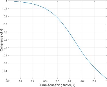
Figure 1: The coherence of ${\bf\Psi}$ in FTN precoding with $L=64$ as a function of the time-squeezing factor, $\xi$.

For a low-complexity approximation, we can again use the OMP algorithm to recover ${\bf s}$ from ${\bf v}$. That is, to solve (23), the OMP algorithm can be used. The resulting approach can provide a good performance if ${\bf\Psi}$ satisfies the RIP and the MMSE filtering provides a good estimate of ${\bf\Psi}{\bf s}$.

V Variational Inference based Detection

In this section, we study a different approach based on variational inference [38] [50] to detect the indices of active symbols. This approach does not solve (19), but finds an approximation of the maximum a posteriori probability (MAP) detection.

V-A Optimal Detection

In order to estimate ${\bf s}$, we can consider the ML approach. From (10), the likelihood function of ${\bf s}$ is given by

$$f({\bf r}\,|\,{\bf s})=\frac{1}{(\pi N_{0})^{L}}\exp\left(-\frac{1}{N_{0}}||{\bf r}-{\cal H}{\bf\Psi}{\bf s}||^{2}\right).$$

The ML estimate can be found as [51]

$$\hat{\bf s} =\operatorname*{\arg\!\max}_{{\bf s}\in\bar{\Sigma}_{Q}}f({\bf r}\,|\,{\bf s})$$ (24)

$$=\operatorname*{\arg\!\min}_{{\bf s}\in\bar{\Sigma}_{Q}}||{\bf r}-{\cal H}{\bf\Psi}{\bf s}||^{2},$$ (25)

where $\bar{\Sigma}_{Q}=\{{\bf s}\,|\,{\bf s}\in\Sigma_{Q},\ s_{l}\in\bar{\cal S}\}$. Here, $\bar{\cal S}={\cal S}\cup\{0\}$. We note that $|\bar{\Sigma}_{Q}|=2^{N_{\rm b}}$, which grows exponentially with $Q$ (from (4)). Since the complexity of the ML detection is proportional to $|\bar{\Sigma}_{Q}|$, it might be computationally prohibitive unless $Q$ is small (i.e., $Q$ is 1 or 2) if an exhaustive search is used.

In order to take into account the sparsity of ${\bf s}$, we can consider the MAP detection. Let $\Pr({\bf s}\,|\,{\bf r})$ represent the a posteriori probability of ${\bf s}$ for given ${\bf r}$. Since

$$\Pr({\bf s}\,|\,{\bf r})\propto f({\bf r}\,|\,{\bf s})\Pr({\bf s}),$$ (26)

where $\Pr({\bf s})$ is the a priori probability of ${\bf s}$ (which can take into account the sparsity of ${\bf s}$), the MAP detection to find ${\bf s}$ that maximizes $\Pr({\bf s}\,|\,{\bf r})$ can be given by

$$\hat{\bf s}=\operatorname*{\arg\!\max}_{{\bf s}\in\bar{\Sigma}_{Q}}\Pr({\bf s}\,|\,{\bf r}).$$ (27)

Like the ML detection, if an exhaustive search is considered to perform the MAP detection, the complexity becomes prohibitively high.

V-B Variational Inference

Since the optimal detection (ML or MAP) requires a high computational complexity, we may need to consider a low-complexity approach to find an approximation. To this end, we can consider the variational inference [38] [50] [52], which is a well-known machine learning technique.

The variation inference is to obtain an approximate solution to the MAP problem using variational distributions of ${\bf s}$. Let $\rho_{n}(s_{n})$ be the distribution of $s_{n}\in\bar{\cal S}$. In addition, ${\cal R}$ denotes the set of the distributions of $\rho_{n}(s)$ for $s\in\bar{\cal S}$. Furthermore, we assume that the $s_{n}$’s are independent. Thus, we have

$$\rho({\bf s})=\prod_{n=0}^{N-1}\rho_{n}(s_{n}),$$

which results in the mean-field approximation in variational inference [50]. An approximation of the a posteriori probability, $\Pr({\bf s}\,|\,{\bf r})$, can be obtained through the following optimization:

$$\rho^{*}=\operatorname*{\arg\!\min}_{\rho\in{\cal R}^{N}}{\rm KL}\left(\rho({\bf s})||\Pr({\bf s}\,|\,{\bf r})\right),$$ (28)

where ${\rm KL}(\cdot)$ is the Kullback-Leibler (KL) divergence [53], which is defined as

$${\rm KL}(\rho({\bf s})||f({\bf s}))=\sum_{\bf s}\rho({\bf s})\ln\frac{\rho({\bf s})}{f({\bf s})}.$$

Here, $f({\bf s})$ is any distribution of ${\bf s}$ with $f({\bf s})>0$ for all ${\bf s}\in\bar{\cal S}^{N}$. Since the KL divergence is to measure the difference between two probability distributions, $\rho^{*}({\bf s})$ in (28) becomes an approximation of $\Pr({\bf s}\,|\,{\bf r})$. Then, the MAP detection can be carried out with $\rho^{*}({\bf s})$ instead of $\Pr({\bf s}\,|\,{\bf r})$. Thanks to the assumption that the $s_{n}$’s are independent, $s_{n}$ can be estimated as follows:

$$\hat{s}_{n}=\operatorname*{\arg\!\max}_{s_{n}\in\bar{\cal S}}\rho_{n}^{*}(s_{n}).$$

If $\hat{s}_{n}\neq 0$, $s_{n}$ is detected as an active symbol and its value in the $M$-ary constellation, ${\cal S}$, can also be obtained.

Note that since the sparsity of ${\bf s}$ is $Q$, it has to be taken into account. To this end, let $\tilde{\rho}_{n}=1-\rho_{n}(0)$. In addition, denote by $a(n)$ the index of the $n$th largest one among $\{\tilde{\rho}_{0},\ldots,\tilde{\rho}_{N-1}\}$, i.e., $\tilde{\rho}_{a(0)}\geq\ldots\geq\tilde{\rho}_{a(N-1)}$. Then, the index set of $Q$ active symbols becomes $\{a(0),\ldots,a(Q-1)\}$. We can also readily impose the constraint of structured IM if ${\bf s}$ is a structured IM signal in choosing $Q$ active symbols. Furthermore, soft-decisions on the IM bits can be found as $\rho(\cdot)$ is a probability, which might be useful for decoding when a channel code is used.

V-C CAVI Algorithm with Gaussian Approximation

As shown in [52], the minimization of the KL divergence in (28) is equivalent to the maximization of the evidence lower bound (ELBO), which is given by

$${\rm ELBO}(\rho)={\mathbb{E}}[\ln f({\bf r},{\bf s})]-{\mathbb{E}}[\ln\Pr({\bf s})],$$ (29)

where the expectation is carried out over ${\bf s}$. Let ${\bf s}_{-n}=[s_{1}\ \ldots\ s_{n-1}\ s_{n+1}\ \ldots\ s_{N}]^{\rm T}$. Then, for given ${\bf s}_{-n}$, it can be shown that

$$\rho_{n}\propto\exp\left({\mathbb{E}}_{-n}[\ln f(s_{n}\,|\,{\bf s}_{-l},{\bf r})]\right),$$ (30)

where the expectation, denoted by ${\mathbb{E}}_{-n}$, is carried out over ${\bf s}_{-n}$. The coordinate ascent variational inference (CAVI) algorithm [50, 52] is to update $\rho_{n}$, $n=0,\ldots,N-1$, while the other variational distributions, $\rho_{-n}$, are fixed. The CAVI algorithm requires a number of iterations, denoted by $N_{\rm run}$.

To carry out the updating in (30), we need to have a closed-form expression for ${\mathbb{E}}_{-n}[\ln f(s_{n}\,|\,{\bf s}_{-n},{\bf r})]$. Unfortunately, since $f(s_{n}\,|\,{\bf s}_{-n},{\bf r})$ is a Gaussian mixture and it is difficult to find a closed-form expression. However, as shown in [54], a suboptimal approach is available with the Gaussian approximation where an active symbol $s_{n}$ is assumed to be a CSCG random variable. In particular, let $s_{l}$ be a zero-mean CSCG random variable with variance $\sigma_{s}^{2}$ when $s_{l}\neq 0$. Define the activity variable, $x_{l}$, as

$$x_{l}=\left\{\begin{array}[]{ll}1,&\mbox{if $s_{l}\neq 0$}\cr 0,&\mbox{if $s_{l}=0$.}\cr\end{array}\right.$$

For convenience, let ${\bf A}={\cal H}{\bf\Psi}$ and denote by ${\bf a}_{l}$ the $l$th column of ${\bf A}$. Furthermore, let $\chi_{l}^{(i)}(x_{l})$ be the estimate of $\Pr(x_{l})$ in the $i$th iteration of the CAVI algorithm, where the superscript $(i)$ represents the $i$th iteration (i.e., $i$ is used for the iteration index). Under the Gaussian assumption of $s_{l}$, the CAVI updating rule for $\chi_{l}^{(i)}(x_{l})$ is given by

$$\chi_{l}^{(i)}(x_{l}) =e^{-{\bf r}^{\rm H}{\bf R}_{l}^{(i)}(x_{l})^{-1}{\bf r}-\ln\det({\bf R}_{l}^{(i)}(x_{l}))},\ x_{l}\in\{0,1\},$$ (31)

where

$${\bf R}_{l}^{(i)}(x_{l}) ={\bf a}_{l}{\bf a}_{l}^{\rm H}x_{l}+\sum_{t<l}{\bf a}_{t}{\bf a}_{t}^{\rm H}\bar{\chi}_{t}^{(i)}$$ (32)

$$\quad+\sum_{t>l}{\bf a}_{t}{\bf a}_{t}^{\rm H}\bar{\chi}_{t}^{(i-1)}+\gamma^{-1}{\bf I},$$ (33)

where $\bar{\chi}_{l}^{(i)}$ is the normalized version of $\chi_{l}^{(i)}(x_{l})$, which is given by $\bar{\chi}_{l}^{(i)}=\frac{\chi_{l}^{(i)}(1)}{\chi_{l}^{(i)}(0)+\chi_{l}^{(i)}(1)}$. The resulting CAVI algorithm provides the support of ${\bf s}$. Once the support of ${\bf s}$ is found, we can easily estimate the non-zero elements of ${\bf s}$ from ${\bf r}$. In [54], detailed derivations are presented and it is also shown that the complexity per iteration is $O(L^{2}N)$. From this, we can see that the complexity grows linearly with $N$ (which is similar to the OMP algorithm) and its complexity is higher than that of the OMP algorithm by a factor of $LN_{\rm run}$.

VI Generalization of SCIM to Multiple Access for Low-Rate Devices

In this section, SCIM with precoding is generalized to multiple access channel so that multiple devices can be supported in the same resource block.

Suppose that there are $K$ devices to transmit their signals to the BS. Let ${\cal H}_{k}$ and ${\bf\Psi}_{k}\in{\mathbb{C}}^{L\times N}$ denote the channel and precoding matrices of device $k$, respectively. Then, the received signal at the BS is given by

$${\bf r}=\sum_{k=1}^{K}{\cal H}_{k}{\bf\Psi}_{k}{\bf s}_{k}+{\bf n}.$$ (34)

Let

$${\bf A} =[({\cal H}_{1}{\bf\Psi}_{1})\ \cdots\ ({\cal H}_{K}{\bf\Psi}_{K})]\in{\mathbb{C}}^{L\times NK}$$ (35)

$${\bf z} =[{\bf s}_{1}^{\rm T}\ \ldots\ {\bf s}_{K}^{\rm T}]^{\rm T}\in{\mathbb{C}}^{NK\times 1}.$$ (36)

Then, it can be shown that

$${\bf r}={\bf A}{\bf z}+{\bf n}.$$ (37)

If each device uses the structured IM with $Q$ active symbols (and $N=DQ$), ${\bf z}$ can be seen as a structured IM with $QK$ active symbols. It is clear that both the OMP and CAVI algorithms can be employed at the BS to detect the signals from $K$ devices, i.e., $QK$-sparse signal ${\bf z}$, from ${\bf r}$. For example, the CAVI algorithm can provide an approximate solution to the MAP detection by obtaining an approximate a posteriori probability as follows:

$$\rho({\bf z})\approx\Pr({\bf z}\,|{\bf r}).$$

Note that since the MMSE filtering is not applicable to the superposition of precoded signals, the approach in Subsection IV-C cannot be used.

FTN signaling can be applied to SCIM for multiple access. In particular, according to (36), since the size of ${\bf A}$ is $L\times NK$, the system time-squeezing factor becomes $\xi=\frac{L}{NK}$ with the following precoding matrix for device $k$:

$$[{\bf\Psi}_{k}]_{l,n}=g((l-(nK+k-1)\xi)T),\ k=1,\ldots,K,$$ (38)

where $l\in\{0,\ldots,L-1\}$ and $n\in\{0,\ldots,N-1\}$. Let $l_{k}=l-\xi(k-1)$. Then, from (38), we have

$$[{\bf\Psi}_{k}]_{l,n}=g((l_{k}-nK\xi)T),$$ (39)

which shows that the effective time-squeezing factor at a device becomes $K\xi=\frac{L}{N}$. Thus, if $N<L$, the device’s transmission rate becomes lower than the BS’s sampling rate (or Nyquist rate). For example, if $L=64$, $K=2$, and $(Q,D)=(5,8)$, we have $N=40$. Thus, the system time-squeezing factor is $\frac{64}{80}<1$, while the device’s time-squeezing factor $K\xi$ is $\frac{64}{40}>1$. In Fig. 2, SCIM waveforms transmitted from two low-rate devices are illustrated when $L=64$ and $K=2$ with $(Q,D)=(5,8)$. The BS would be able to recover the two sparse signals from $L=64$ samples per block by solving (37).

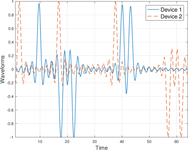
Figure 2: Transmitted SCIM waveforms transmitted from two low-rate devices when $L=64$ and $K=2$ with $(Q,D)=(5,8)$.

As shown above, the generalization of SCIM with FTN precoding to multiple access channel can play a key role in supporting a number of devices with a limited spectrum by allowing multiple IoT devices of low transmission rates to share the same radio resource block. However, there are other issues to be addressed as follows.

• Channel Estimation: As shown in (36), the BS needs to know ${\bf A}$, which means that it requires to estimate ${\cal H}_{k}$ since ${\bf\Psi}_{k}$ is known. As in [6] [7], prior to data transmissions, a handshaking procedure can be used for random access where the channel estimation can also be carried out as each active device is to transmit a preamble. In particular, once the BS is able to detect the preambles transmitted by multiple active devices without any collision, it should be able to estimate their channels (taking the preambles as pilot signals). Then, for data transmissions, multiple active devices can employ SCIM (with different precoding matrices) to transmit their signals in the same radio resource block.

• When FTN precoding is used, in (39), each device has the same effective time-squeezing factor, $\frac{L}{N}$. In fact, it is also possible to have a different time-squeezing factor by allowing a different number columns of ${\bf\Psi}_{k}$, which is denoted by $N_{k}$. Then, the system time-squeezing factor becomes $\frac{L}{\sum_{k=1}^{K}N_{k}}$, while device $k$’s effective time-squeezing factor is $\frac{L}{N_{k}}$. In other words, supporting multiple devices of different transmission rates is possible using SCIM with precoding. This feature might be crucial to support a wide range of IoT devices that may have different transmission rates.

VII Simulation Results

In this section, we present simulation results of SCIM when 4-QAM (in this case, $M=4$) is used for active symbols with ${\cal S}=\{\pm 1\pm j\}$ with the structured IM. For the multipath channel, we assume that the channel coefficients are independent and $h_{p}\sim{\cal C}{\cal N}(0,1/P)$, $p=0,\ldots,P-1$, i.e., a multipath Rayleigh fading channel is considered. The signal-to-noise ratio (SNR) is defined as $\frac{E_{\rm b}}{N_{0}}$, where $E_{\rm b}$ represents the bit energy that is given by

$$E_{\rm b}=\frac{Q\sigma_{s}^{2}}{\tilde{N}_{\rm im}+Q\log_{2}M}.$$

Here, $\sigma_{s}^{2}=2$ as 4-QAM is used. We also assume FTN precoding for SCIM. For the signal detection, the following 3 different approaches are considered at the receiver of BS: (i) the OMP detector that uses the OMP algorithm to solve (19); (ii) the OMP-MMSE detector that employs the MMSE filtering with the OMP algorithm to solve (23); (iii) the CAVI detector that is based on the CAVI algorithm (unless stated otherwise, we assume that the number of iterations for the CAVI detector is set to $N_{\rm run}=4$). To see the performance, we consider the index error rate (IER) that is the probability of erroneously detection of any index of active symbols.

We first consider SCIM with FTN precoding for a single device. Fig. 3 shows the IERs of the three detectors as functions of SNR with two different sets of parameters’ values. In Fig. 3 (a), we consider $L=128$ and $N=160$ with $P=6$ and $(D,Q)=(32,5)$. In this case, we have $\tilde{N}_{\rm im}=25$ bits. On the other hand, in Fig. 3 (b), we consider $L=64$ and $N=80$ with $P=4$ and $(D,Q)=(8,10)$, where $\tilde{N}_{\rm im}=30$ bits. Clearly, the size of the system in Fig. 3 (b) is smaller than that in Fig. 3 (a), while the former transmits slightly more bits than the latter. As a result, the performance of the system in Fig. 3 (a) in terms of IER is better than that in Fig. 3 (b). We note that the CAVI detector outperforms the other detectors, i.e., the OMP and OMP-MMSE detectors, at the cost of a higher computational complexity. It is also interesting to see that the OMP-MMSE detector can provide a comparable performance to the CAVI detector, while the OMP detector suffers from the error floor. Thus, we need to use the OMP-MMSE or CAVI detector at a high SNR to avoid the error floor.

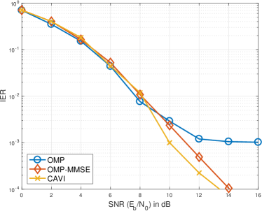
(a)

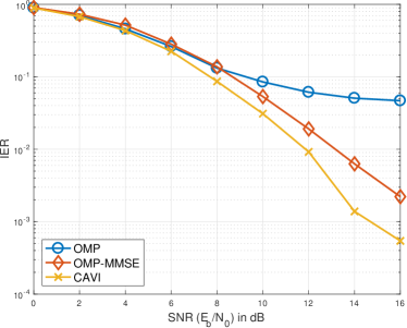
(b)

Figure 3: IER as a function of SNR: (a) $L=128$, $P=6$, $Q=5$, $D=32$; (b) $L=64$, $P=4$, $Q=10$, $D=8$.

For a fixed $L$, SCIM with precoding can transmit more bits as $N$ increases. In particular, with a fixed $D$, $\tilde{N}_{\rm im}$ can grow linearly with $N$ or $Q$ as $\tilde{N}_{\rm im}=Q\log_{2}D=\frac{N}{D}\log_{2}D$. In Fig. 4 (a), we present the IER as a function of sparsity $Q$ (or $N$) with fixed $D=8$ when $L=64$, $P=4$, and SNR $=16$dB, where a trade-off between the number of bits transmitted by IM (i.e., $\tilde{N}_{\rm im}$) and the performance of IER is shown. That is, the increase of $\tilde{N}_{\rm im}$ results in a poor IER performance. We note that the performance of the OMP-MMSE detector is close to that of the CAVI detector when $Q$ is small. However, as $Q$ increases, the performance of the OMP-MMSE detector approaches that of the OMP detector. Thus, when a sufficiently low IER is desirable with a small $Q$, the OMP-MMSE detector (instead of the CAVI detector) can be used as it can provide a good performance with low-complexity.

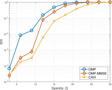
(a)

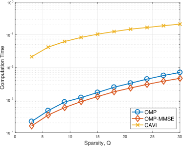
(b)

Figure 4: IER and computation time of the 3 different detectors as functions of $Q$ (or $N$) with fixed $D=8$ when $L=64$, $P=4$, and SNR $=16$dB: (a) IER; (b) computation time (obtained by “tic” and “toc” commands of MATLAB).

In Fig. 4 (b), we show the computation times of the 3 different detectors with the same parameter set as those used in Fig. 4 (a). It is shown that the computation time increases with $Q$ or $N$ and the computation time of the CAVI detector is much higher than those of the OMP and OMP-MMSE detectors as expected. In particular, as mentioned earlier, the complexity order of the CAVI algorithm is $LN_{\rm run}$ times higher than that of the OMP algorithm, so the CAVI detector requires a higher computation time when comparing the OMP detector by $LN_{\rm times}=256$ times or a factor of $10^{2}$, which is clearly shown in Fig. 4 (b).

Note that in Fig. 4 (b), the computation time of the OMP detector is higher than that of the OMP-MMSE detector. This is due to the different measurement matrices in (19) and (23). In (23), ${\bf\Psi}$ with FTN signaling has a number of zeros, which allows efficient pseudo-inverse operations in the OMP algorithm and results in a low computation time. Thus, the OMP-MMSE detector is better than the OMP detector in terms of performance as well as computational complexity.

With FTN precoding, the time-squeezing factor, $\xi$, affects performance. To see this, we show the IER as a function of $\xi$ in Fig. 5 with $Q=4$, $L=64$, $P=4$, and SNR $=16$dB. Note that since $Q$ is fixed, as $\xi$ increases, $N$ or $D$ also increases, which also results in the increase of $\tilde{N}_{\rm im}$. It is shown that the time-squeezing factor cannot be too small to provide a reasonable performance. For example, with $\xi=0.5$, an IER of $10^{-2}$ can be achieved. However, if $\xi$ becomes smaller than $0.5$, the IER becomes too high.

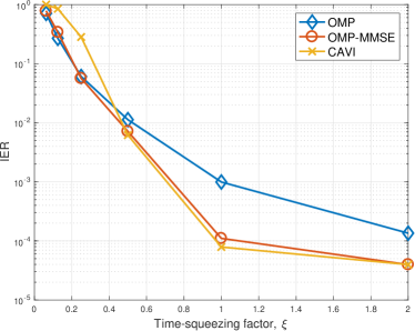
Figure 5: IER as a function of the time-squeezing factor $\xi$ with $Q=4$, $L=64$, $P=4$, and SNR $=16$dB.

We now consider the use of SCIM with FTN precoding to support multiple low-rate devices in the same radio resource block. As mentioned earlier, in this case, the OMP-MMSE detector cannot be used. Thus, for a good performance with a reasonable computational complexity, we may need to use the CAVI detector. Since the CAVI detector is based on an iterative algorithm, its performance depends on the number of iterations, $N_{\rm run}$. In Fig. 6, we show the IER of the CAVI detector as a function of the number of iterations, $N_{\rm run}$, when $L=64$, $P=4$, $K=2$, $(Q,D)=(5,8)$, and SNR $=16$dB. We can see that 3 or 4 iterations are sufficient for the convergence at a medium or high SNR. Thus, as before, $N_{\rm run}$ is set to 4 in the rest of simulations.

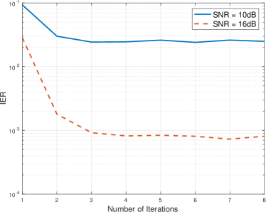
Figure 6: IER of CAVI as a function of the number of iterations, $N_{\rm run}$ when $L=64$, $P=4$, $K=2$, $(Q,D)=(5,8)$, and SNR $=16$dB.

In Fig. 7, we show the IER of SCIM with multiple devices as a function of SNR when $L=64$, $P=4$, $Q=5$, $D=8$, and $K=2$. In this case, the transmission rate at each device is lower than the Nyquist rate at the receiver by a factor of $40/64=0.625$, and each device has $\tilde{N}_{\rm im}=5\log_{2}8=15$ bits to be transmitted by IM. In addition, since 4-QAM is used for active symbols, the total number of bits per block per device is $15+5\log_{2}4=25$ bits. At an SNR of 16dB, the CAVI detector can provide an IER lower than $10^{-3}$ and the OMP detector can achieve an IER slightly lower than $10^{-1}$. Clearly, it demonstrates that the simple OMP detector cannot be used, but a more complicated detector, e.g., the CAVI detector, is required to achieve a good performance.

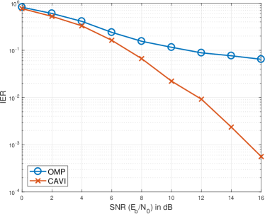
Figure 7: IER of SCIM with multiple devices as a function of SNR when $L=64$, $P=4$, $Q=5$, $D=8$, and $K=2$.

Fig. 8 shows the IER of SCIM with multiple devices as a function of $K$ when $L=64$, $P=4$, $Q=3$, $D=8$, and SNR $=16$ dB. Since $D$ and $Q$ are fixed, each device can transmit $\tilde{N}_{\rm im}=3\log_{2}8=9$ bits by IM regardless of $K$, and the transmission rate at each device is lower than the Nyquist rate at the receiver by a factor of $24/64=0.375$ (since $N=QD=24$). It is shown that as $K$ increases, the IER increases, which demonstrates a trade-off between the performance and the number of devices to be supported. Clearly, the number of devices, $K$, is to be limited for a reasonably good performance in terms of IER. For example, at a target IER of $10^{-2}$, $K$ can be up to 5 if the CAVI detector is used.

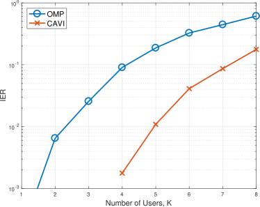
Figure 8: IER of SCIM with multiple devices as a function of $K$ when $L=64$, $P=4$, $Q=3$, $D=8$, and SNR $=16$ dB.

The impact of $L$ on the performance of SCIM with multiple devices in terms of IER is shown in Fig. 9 when $K=2$, $P=4$, $Q=5$, $D=8$, and SNR $=16$ dB. Since $Q$ and $D$ are fixed, $N=40$ is also fixed at each device. Thus, as $L$ increases, we can assume that the system bandwidth increases and the spectral efficiency decreases. Thus, in Fig. 9, we can see that the IER decreases at the cost of spectral efficiency (i.e., lowering the spectral efficiency results in a lower IER).

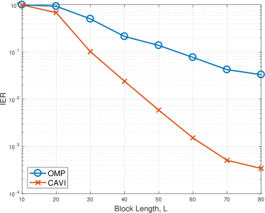
Figure 9: IER of SCIM with multiple devices as a function of $L$ when $K=2$, $P=4$, $Q=5$, $D=8$, and SNR $=16$ dB.

As mentioned earlier, an advantage of SCIM over OFDM-IM is the path diversity gain. Thus, it is expected to see a better performance as $P$ increases. In Fig. 10, the IER is shown as a function of the number of multipaths, $P$, with $L=64$, $K=2$, $Q=5$, $D=8$, and SNR $=16$ dB. As expected, due to a higher path diversity gain, a lower IER can be achieved with increasing $P$ when the CAVI detector is used. On the other hand, the OMP detector does not provide an improved performance as $P$ increases. This demonstrates that in order to fully exploit the path diversity gain, an optimal detector or an approximate optimal detector has to be used.

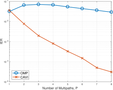
Figure 10: IER of SCIM with multiple devices as a function of $P$ when $L=64$, $K=2$, $Q=5$, $D=8$, and SNR $=16$ dB.

VIII Concluding Remarks

In this paper, we studied SCIM that is an application of IM to SC systems for IoT uplink as it has several advantages, e.g., low PAPR, path diversity gain, no inverse FFT operation required, compared to OFDM-IM. To increase the number of information bits transmitted by IM, precoding was applied to SCIM. In particular, FTN precoding has been considered. We also generalized SCIM with precoding to multiple access channel so that multiple devices can share the same radio resource block for uplink transmissions. With FTN precoding, we showed that devices can have lower transmission rates than the receiver’s sampling rate (Nyquist rate), which might be useful when a device needs to lower its clock frequency for energy saving. We also derived different detectors for sparse signal detection including the CAVI detector that can provide an approximate solution to the (optimal) MAP detection.

There are a number of further research works for SCIM with precoding. For example, optimal precoding matrices can be designed under various constraints. In particular, when devices have different transmission rates, the design of optimal precoding matrices might be an interesting and important topic. Channel coding can also be considered. Since the CAVI detector can provide soft-decisions, channel decoding can be performed with soft-decisions together with the CAVI detector. Furthermore, in each iteration of the CAVI algorithm, channel decoding can be performed, which can result in a fast convergence rate as well as an improved performance.

References

- [1] L. Atzori, A. Iera, and G. Morabito, “The Internet of Things: A survey,” Comput. Netw., vol. 54, pp. 2787–2805, Oct. 2010.
- [2] ITU-T, Y.2060: Overview of the Internet of things, June 2012.
- [3] A. Al-Fuqaha, M. Guizani, M. Mohammadi, M. Aledhari, and M. Ayyash, “Internet of Things: A survey on enabling technologies, protocols, and applications,” IEEE Communications Surveys Tutorials, vol. 17, pp. 2347–2376, Fourthquarter 2015.
- [4] S. K. Sharma, T. E. Bogale, S. Chatzinotas, X. Wang, and L. B. Le, “Physical layer aspects of wireless IoT,” in 2016 International Symposium on Wireless Communication Systems (ISWCS), pp. 304–308, Sept 2016.
- [5] J. A. Gutierrez, E. H. Callaway, and R. Barrett, IEEE 802.15.4 Low-Rate Wireless Personal Area Networks: Enabling Wireless Sensor Networks. New York, NY, USA: IEEE Standards Office, 2003.
- [6] 3GPP TR 37.868 V11.0, Study on RAN improvments for machine-type communications, October 2011.
- [7] 3GPP TS 36.321 V13.2.0, Evolved Universal Terrestrial Radio Access (E-UTRA); Medium Access Control (MAC) protocol specification, June 2016.
- [8] Y. . E. Wang, X. Lin, A. Adhikary, A. Grovlen, Y. Sui, Y. Blankenship, J. Bergman, and H. S. Razaghi, “A primer on 3GPP narrowband Internet of Things,” IEEE Communications Magazine, vol. 55, pp. 117–123, March 2017.
- [9] E. Dahlman, S. Parkvall, and J. Skold, 4G: LTE/LTE-Advanced for Mobile Broadband, 2nd Edition. Academic Press, 2013.
- [10] E. Basar, U. Aygolu, E. Panayirci, and H. Poor, “Orthogonal frequency division multiplexing with index modulation,” IEEE Trans. Signal Processing, vol. 61, pp. 5536–5549, Nov 2013.
- [11] R. Abu-alhiga and H. Haas, “Subcarrier-index modulation OFDM,” in Personal, Indoor and Mobile Radio Communications, 2009 IEEE 20th International Symposium on, pp. 177–181, Sept 2009.
- [12] L. Xiao, B. Xu, H. Bai, Y. Xiao, X. Lei, and S. Li, “Performance evaluation in PAPR and ICI for ISIM-OFDM systems,” in 2014 International Workshop on High Mobility Wireless Communications, pp. 84–88, Nov 2014.
- [13] R. Fan, Y. J. Yu, and Y. L. Guan, “Generalization of orthogonal frequency division multiplexing with index modulation,” IEEE Trans. Wireless Communications, vol. 14, pp. 5350–5359, Oct 2015.
- [14] Y. Ko, “A tight upper bound on bit error rate of joint OFDM and multi-carrier index keying,” IEEE Communications Letters, vol. 18, pp. 1763–1766, Oct 2014.
- [15] R. Y. Mesleh, H. Hass, S. Sinanovic, C. W. Ahn, and S. Yun, “Spatial modulation,” IEEE Trans. Veh. Technol., vol. 57, pp. 2228–2241, July 2008.
- [16] J. Jeganathan, A. Ghrayeb, and L. Szczecinski, “Spatial modulation: optimal detection and performance analysis,” IEEE Commun. Letters, vol. 12, pp. 545–547, Aug. 2008.
- [17] M. D. Renzo, H. Haas, and P. M. Grant, “Spatial modulation for multiple-antenna wireless systems: a survey,” IEEE Communications Magazine, vol. 49, pp. 182–191, December 2011.
- [18] E. Basar, “Index modulation techniques for 5G wireless networks,” IEEE Communications Magazine, vol. 54, pp. 168–175, July 2016.
- [19] J. Choi and Y. Ko, “Compressive sensing based detector for sparse signal modulation in precoded OFDM,” in Proc. IEEE ICC, pp. 4536–4540, June 2015.
- [20] J. Choi, “Sparse index multiple access,” in 2015 IEEE Global Conference on Signal and Information Processing (GlobalSIP), pp. 324–327, Dec 2015.
- [21] J. Choi, “Sparse index multiple access for multi-carrier systems with precoding,” J. Communications and Neworks, vol. 18, pp. 3226–3237, June 2016.
- [22] D. Donoho, “Compressed sensing,” IEEE Trans. Information Theory, vol. 52, pp. 1289–1306, April 2006.
- [23] E. Candes, J. Romberg, and T. Tao, “Robust uncertainty principles: exact signal reconstruction from highly incomplete frequency information,” IEEE Trans. Information Theory, vol. 52, pp. 489–509, Feb 2006.
- [24] E. Basar, “Multiple-input multiple-output OFDM with index modulation,” IEEE Signal Processing Letters, vol. 22, pp. 2259–2263, Dec 2015.
- [25] B. Zheng, M. Wen, E. Basar, and F. Chen, “Multiple-input multiple-output ofdm with index modulation: Low-complexity detector design,” IEEE Trans. Signal Processing, vol. 65, pp. 2758–2772, June 2017.
- [26] S. Gao, M. Zhang, and X. Cheng, “Precoded index modulation for multi-input multi-output ofdm,” IEEE Trans. Wireless Communications, vol. 17, pp. 17–28, Jan 2018.
- [27] E. Basar, “OFDM with index modulation using coordinate interleaving,” IEEE Wireless Communications Letters, vol. 4, pp. 381–384, Aug 2015.
- [28] Y. Liu, F. Ji, H. Yu, F. Chen, D. Wan, and B. Zheng, “Enhanced coordinate interleaved OFDM with index modulation,” IEEE Access, vol. 5, pp. 27504–27513, 2017.
- [29] Q. Li, M. Wen, E. Basar, H. V. Poor, B. Zheng, and F. Chen, “Diversity enhancing multiple-mode OFDM with index modulation,” IEEE Trans. Communications, vol. 66, pp. 3653–3666, Aug 2018.
- [30] J. Choi, “Coded OFDM-IM with transmit diversity,” IEEE Trans. Communications, vol. 65, pp. 3164–3171, July 2017.
- [31] J. Choi and Y. Ko, “TCM for OFDM-IM,” IEEE Wireless Communications Letters, vol. 7, pp. 50–53, Feb 2018.
- [32] S. Sugiura, T. Ishihara, and M. Nakao, “State-of-the-art design of index modulation in the space, time, and frequency domains: Benefits and fundamental limitations,” IEEE Access, vol. 5, pp. 21774–21790, 2017.
- [33] J. Choi, “Single-carrier index modulation and CS detection,” in 2017 IEEE International Conference on Communications (ICC), pp. 1–6, May 2017.
- [34] M. Nakao, T. Ishihara, and S. Sugiura, “Single-carrier frequency-domain equalization with index modulation,” IEEE Communications Letters, vol. 21, pp. 298–301, Feb 2017.
- [35] D. Falconer, S. L. Ariyavisitakul, A. Benyamin-Seeyar, and B. Eidson, “Frequency domain equalization for single-carrier broadband wireless systems,” IEEE Communications Magazine, vol. 40, pp. 58–66, Apr 2002.
- [36] J. E. Mazo, “Faster-than-Nyquist signaling,” The Bell System Technical Journal, vol. 54, pp. 1451–1462, Oct 1975.
- [37] T. Ishihara and S. Sugiura, “Faster-than-Nyquist signaling with index modulation,” IEEE Wireless Communications Letters, vol. 6, pp. 630–633, Oct 2017.
- [38] M. I. Jordan, Z. Ghahramani, T. S. Jaakkola, and L. K. Saul, “An introduction to variational methods for graphical models,” Machine Learning, vol. 37, pp. 183–233, Nov 1999.
- [39] J. Spencer, Asymptopia. American Mathematical Society, 2014.
- [40] J. Choi, Adaptive and Iterative Signal Processing in Communications. Cambridge University Press, 2006.
- [41] J. Fan, S. Guo, X. Zhou, Y. Ren, G. Y. Li, and X. Chen, “Faster-than-nyquist signaling: An overview,” IEEE Access, vol. 5, pp. 1925–1940, 2017.
- [42] J. B. Anderson, F. Rusek, and V. Öwall, “Faster-than-Nyquist signaling,” Proceedings of the IEEE, vol. 101, pp. 1817–1830, Aug 2013.
- [43] F. Pancaldi, G. M. Vitetta, R. Kalbasi, N. Al-Dhahir, M. Uysal, and H. Mheidat, “Single-carrier frequency domain equalization,” IEEE Signal Processing Magazine, vol. 25, pp. 37–56, September 2008.
- [44] E. Candes and M. B. Wakin, “An introduction to compressive sampling,” IEEE Signal Processing Magazine, vol. 25, no. 2, pp. 21–30, 2008.
- [45] Y. C. Eldar and G. Kutyniok, Compressed Sensing: Theory and Applications. Cambridge University Press, 2012.
- [46] E. J. Candes, “The restricted isometry property and its implications for compressed sensing,” Comptes Rendus Mathematique, vol. 346, no. 9–10, pp. 589–592, 2008.
- [47] R. Baraniuk, M. Davenport, R. DeVore, and M. Wakin, “A simple proof of the restricted isometry property for random matrices,” Constructive Approximation, vol. 28, no. 3, pp. 253–263, 2008.
- [48] Y. Pati, R. Rezaiifar, and P. Krishnaprasad, “Orthogonal matching pursuit: recursive function approximation with applications to wavelet decomposition,” in Signals, Systems and Computers, 1993. 1993 Conference Record of The Twenty-Seventh Asilomar Conference on, pp. 40–44 vol.1, Nov 1993.
- [49] G. M. Davis, S. G. Mallat, and Z. Zhang, “Adaptive time-frequency decompositions,” Optical Engineering, vol. 33, no. 7, pp. 2183–2191, 1994.
- [50] C. M. Bishop, Pattern Recognition and Machine Learning (Information Science and Statistics). Berlin, Heidelberg: Springer-Verlag, 2006.
- [51] J. Choi, Optimal Combining and Detection. Cambridge University Press, 2010.
- [52] D. M. Blei, A. Kucukelbir, and J. D. McAuliffe, “Variational inference: A review for statisticians,” Journal of the American Statistical Association, vol. 112, no. 518, pp. 859–877, 2017.
- [53] T. M. Cover and J. A. Thomas, Elements of Inform. Theory. NJ: John Wiley, second ed., 2006.
- [54] J. Choi, “A variational inference based detection method for repetition coded generalized spatial modulation,” IEEE Trans. Communications, pp. 1–1, 2018 (to be published).