SmeftFR – Feynman rules generator for the Standard Model Effective Field Theory

Abstract

We present SmeftFR, a Mathematica package designed to generate the Feynman rules for the Standard Model Effective Field Theory (SMEFT) including the complete set of gauge invariant operators up to dimension 6. Feynman rules are generated with the use of FeynRules package, directly in the physical (mass eigenstates) basis for all fields. The complete set of interaction vertices can be derived including all or any chosen subset of SMEFT operators. As an option, the user can also choose preferred gauge fixing, generating Feynman rules in unitary or $R_{\xi}$-gauges (the latter include generation of ghost vertices). Further options allow to treat neutrino fields as massless Weyl or massive Majorana fermions. The derived Lagrangian in the mass basis can be exported in various formats supported by FeynRules, such as UFO, FeynArts, etc. Initialisation of numerical values of $d=6$ Wilson coefficients used by SmeftFR is interfaced to WCxf format. The package also includes dedicated Latex generator allowing to print the result in clear human-readable form. SmeftFR can be downloaded from the address www.fuw.edu.pl/smeft.

PROGRAM SUMMARY

Manuscript Title:
SmeftFR – Feynman rules generator for the Standard Model Effective Field Theory
Authors: Athanasios Dedes, Michael Paraskevas, Janusz Rosiek, Kristaq Suxho, Lampros Trifyllis
Program Title: SmeftFR v2.0
Journal Reference:
Catalogue identifier:
Licensing provisions: None
Programming language: Mathematica 11.3 (earlier versions were reported to have problems running this code)
Computer: any running Mathematica
Operating system: any running Mathematica
RAM: allocated dynamically by Mathematica, at least 4GB total RAM suggested
Number of processors used: allocated dynamically by Mathematica
Supplementary material: None
Keywords: Standard Model Effective Field Theory, Feynman rules, unitary and $R_{\xi}$ gauges
Classification:
11.1 General, High Energy Physics and Computing, 4.4 Feynman diagrams, 5 Computer Algebra.
External routines/libraries: Wolfram Mathematica program
Subprograms used: FeynRules v2.3 package
Nature of problem:
Automatised generation of Feynman rules in physical (mass) basis for the Standard Model Effective Field Theory with user defined operator subset and gauge fixing terms selection.
Solution method:
Implementation (as the Mathematica package) of the results of Ref. [1] in the FeynRules package [2], including dynamic “model files” generation.
Restrictions: None
Unusual features: None
Additional comments: None
Running time: depending on control variable settings, from few minutes for a selected subset of few SMEFT operators and Feynman rules generation up to several hours for generating UFO output for maximum 60-operator set (using Mathematica 11.3 running on a personal computer)

1 Introduction

Despite lack of direct discoveries of new particles at LHC, indirect experiments searching for cosmological dark matter and dark energy, neutrino masses and mixing, heavy meson decays, anomalous magnetic moment of muon, point to existence of new physics phenomena that go beyond the Standard Model (SM) [1, 2, 3] of particle physics. It has become customary in recent years to parameterise the potential effects of such New Physics (NP) in terms of the so-called SM Effective Field Theory (SMEFT) [4, 5, 6]. In this theory, SM is extended by a complete set of gauge invariant operators constructed only by the SM fields which are considered to be light in mass with respect to, yet unknown, particles responsible for NP phenomena. Such (non-renormalisable) operators can be classified according to their growing mass dimension, with couplings (usually called Wilson coefficients) suppressed by respectively inverse powers of a typical mass scale $\Lambda$ of the NP extension.

As observable effects of new operators are typically suppressed by powers of $v/\Lambda$ (where $v$ is the true vacuum expectation value of the Higgs field), in many analyses it is sufficient to restrict the maximal dimension of new operators to $d\leq 6$. Classification of the complete independent set of the gauge invariant operators up to $d=6$ was conducted in an older study by Buchmüller and Wyler [8] and more recently put in a non-redundant form in ref. [9], where the basis of such operators, usually referred as the “Warsaw basis”, has been given. Suppressing the flavour indices of the fields and not counting hermitian conjugated operators, Warsaw basis contains 59+1 baryon-number conserving and 4 baryon-number violating operators.

In its most general version, SMEFT is a hugely complicated model. Including all possible CP- and flavour-violating interactions, it contains 2499 free parameters. Due to large number and complicated structure of new terms in the Lagrangian, theoretical calculations of physical processes within the SMEFT can be very challenging — it is enough to notice that the number of primary vertices when SMEFT is quantised in $R_{\xi}$-gauges, printed for the first time in ref. [10], is almost 400 without counting the hermitian conjugates. Thus, it is important to develop technical methods and tools facilitating such calculations, starting from developing the universal set of the Feynman rules for propagators and vertices for physical fields, after spontaneous symmetry breaking (SSB) of the full effective theory. The initial version of relevant package, SmeftFR v1, was announced and briefly described for the first time in Appendix B of ref. [10]. In this paper we present SmeftFR v2.0, a Mathematica symbolic language package generating Feynman rules in several formats, based on the formulae developed in ref. [10]. Comparing to version 1, the new code has been extended with a number of additional options and capabilities. It has also been made and tested to be compatible with many other publicly available high-energy physics related computer codes accepting standardised input and output data formats. Features of the presented package contain:

• SmeftFR is able to generate interactions in the most general form of the SMEFT Lagrangian, without any restrictions on the structure of flavour violating terms and on CP-, lepton- or baryon-number conservation. Feynman rules are expressed in terms of physical SM fields and canonically normalised Goldstone and ghost fields. Expressions for interaction vertices are analytically expanded in powers of inverse New Physics scale $1/\Lambda$, with all terms of dimension higher than $d=6$ consistently truncated.

• SmeftFR is written as an overlay to FeynRules package [11], used as the engine to generate Feynman rules.

• Including the full set of SMEFT parameters in model files for FeynRules may lead to very slow computations. SmeftFR can generate FeynRules model files dynamically, including only the user defined subset of higher dimension operators. It significantly speeds up the calculations and produces simpler final result, containing only the Wilson coefficients relevant for a process chosen to analyse.

• Feynman rules can be generated in the unitary or in linear $R_{\xi}$-gauges by exploiting four different gauge-fixing parameters $\xi_{\gamma},\xi_{Z},\xi_{W},\xi_{G}$ for thorough amplitude checks. In the latter case also all relevant ghost vertices are obtained.

• Feynman rules are calculated first in Mathematica/FeynRules format. They can be further exported in other formats: UFO [12] (importable to Monte Carlo generators like MadGraph5_aMC@NLO 5  [13], Sherpa [14], CalcHEP [15], Whizard [16, 17]), FeynArts [18] which generates inputs for loop amplitude calculators like FeynCalc [19], or FormCalc [20], and others output types supported by FeynRules .

• SmeftFR provides a dedicated Latex generator, allowing to display vertices and analytical expressions for Feynman rules in clear human readable form, best suited for hand-made calculations.

• SmeftFR is interfaced to the WCxf format [21] of Wilson coefficients. Numerical values of SMEFT parameters in model files can be read from WCxf JSON-type input produced by other computer packages written for SMEFT. Alternatively, SmeftFR can translate FeynRules model files to the WCxf format.

• Further package options allow to treat neutrino fields as massless Weyl or (in the case of non-vanishing dimension-5 operator) massive Majorana fermions, to correct signs in 4-fermion interactions not yet fully supported by FeynRules and to perform some additional operations as described later in this manual.

Feynman rules derived in ref. [10] using the SmeftFR package have been used successfully in many articles including refs. [22, 23, 24, 25, 26, 27, 28, 29, 30, 31, 32] and have passed certain non-trivial tests, such as gauge-fixing parameter independence of the $S$-matrix elements, validity of Ward identities, cancellation of infinities in loop calculations, etc.

We note here in passing, that there is a growing number of publicly available codes performing computations related to SMEFT. These include, Wilson [33], DSixTools [34], MatchingTools [35], which are codes for running and matching Wilson coefficients, SMEFTsim [36], a package for calculating tree level observables, CoDEx [37] or a version of SARAH code [38], that calculate Wilson Coefficients after the decoupling of a more fundamental theory, and finally, DirectDM [39], a code for dark matter EFT. To a degree, these codes (especially the ones supporting WCxf format) can be used in conjunction with SmeftFR. For example, some of them can provide the numerical input for Wilson coefficients of higher dimensional operators at scale $\Lambda$, while others, the running of these coefficients from that scale down to the EW one. Alternatively, Feynman rules evaluated by SmeftFR can be used with Monte Carlo generators to test the predictions of other packages.

The paper is organised as follows. After this Introduction, in Sec. 2 we define the notation and conventions, listing for reference the operator set in Warsaw basis and the formulae for transition to the mass basis. In Sec. 3, we present the structure of the code, installation procedure and available functions. Section 4, contains examples of programs generating the Feynman rules in various formats. We conclude in Sec. 5.

2 SMEFT Lagrangian in Warsaw and mass basis

The classification of higher order operators in SMEFT is done in terms of fields in electroweak basis, before the Spontaneous Symmetry Breaking. SmeftFR uses the so-called “Warsaw basis” [9] as a starting point to calculate physical states in SMEFT and their interactions. For easier reference we copy here from ref. [9] Tables 1 and 2 containing the full collection of $d=6$ operators in Warsaw basis. In addition, we include the single lepton flavour violating dimension-5 operator:

$$Q_{\nu\nu}=\varepsilon_{jk}\varepsilon_{mn}\varphi^{j}\varphi^{m}(l^{\prime k}_{Lp})^{T}\,\mathbb{C}\,l^{\prime n}_{Lr}~{}\equiv~{}(\widetilde{\varphi}^{\dagger}l^{\prime}_{Lp})^{T}\,\mathbb{C}\,(\widetilde{\varphi}^{\dagger}l^{\prime}_{Lr})\;,$$ (2.1)

where $\mathbb{C}$ is the charge conjugation matrix.

$X^{3}$		$\varphi^{6}$  and  $\varphi^{4}D^{2}$		$\psi^{2}\varphi^{3}$
$Q_{G}$	$f^{ABC}G_{\mu}^{A\nu}G_{\nu}^{B\rho}G_{\rho}^{C\mu}$	$Q_{\varphi}$	$(\varphi^{\dagger}\varphi)^{3}$	$Q_{e\varphi}$	$(\varphi^{\dagger}\varphi)(\bar{l}^{\prime}_{p}e^{\prime}_{r}\varphi)$
$Q_{\widetilde{G}}$	$f^{ABC}\widetilde{G}_{\mu}^{A\nu}G_{\nu}^{B\rho}G_{\rho}^{C\mu}$	$Q_{\varphi\Box}$	$(\varphi^{\dagger}\varphi)\raisebox{-1.42262pt}{$\Box$}(\varphi^{\dagger}\varphi)$	$Q_{u\varphi}$	$(\varphi^{\dagger}\varphi)(\bar{q}^{\prime}_{p}u^{\prime}_{r}\widetilde{\varphi})$
$Q_{W}$	$\varepsilon^{IJK}W_{\mu}^{I\nu}W_{\nu}^{J\rho}W_{\rho}^{K\mu}$	$Q_{\varphi D}$	$\left(\varphi^{\dagger}D^{\mu}\varphi\right)^{*}\left(\varphi^{\dagger}D_{\mu}\varphi\right)$	$Q_{d\varphi}$	$(\varphi^{\dagger}\varphi)(\bar{q}^{\prime}_{p}d^{\prime}_{r}\varphi)$
$Q_{\widetilde{W}}$	$\varepsilon^{IJK}\widetilde{W}_{\mu}^{I\nu}W_{\nu}^{J\rho}W_{\rho}^{K\mu}$
$X^{2}\varphi^{2}$		$\psi^{2}X\varphi$		$\psi^{2}\varphi^{2}D$
$Q_{\varphi G}$	$\varphi^{\dagger}\varphi\,G^{A}_{\mu\nu}G^{A\mu\nu}$	$Q_{eW}$	$(\bar{l}^{\prime}_{p}\sigma^{\mu\nu}e^{\prime}_{r})\tau^{I}\varphi W_{\mu\nu}^{I}$	$Q_{\varphi l}^{(1)}$	$(\mbox{${\varphi^{\dagger}i\,\raisebox{5.69054pt}{\boldmath${}^{\leftrightarrow}$}D_{\mu}\,\varphi}$})(\bar{l}^{\prime}_{p}\gamma^{\mu}l^{\prime}_{r})$
$Q_{\varphi\widetilde{G}}$	$\varphi^{\dagger}\varphi\,\widetilde{G}^{A}_{\mu\nu}G^{A\mu\nu}$	$Q_{eB}$	$(\bar{l}^{\prime}_{p}\sigma^{\mu\nu}e^{\prime}_{r})\varphi B_{\mu\nu}$	$Q_{\varphi l}^{(3)}$	$(\mbox{${\varphi^{\dagger}i\,\raisebox{5.69054pt}{\boldmath${}^{\leftrightarrow}$}D_{\mu}^{\,I}\,\varphi}$})(\bar{l}^{\prime}_{p}\tau^{I}\gamma^{\mu}l^{\prime}_{r})$
$Q_{\varphi W}$	$\varphi^{\dagger}\varphi\,W^{I}_{\mu\nu}W^{I\mu\nu}$	$Q_{uG}$	$(\bar{q}^{\prime}_{p}\sigma^{\mu\nu}\mathcal{T}^{A}u^{\prime}_{r})\widetilde{\varphi}\,G_{\mu\nu}^{A}$	$Q_{\varphi e}$	$(\mbox{${\varphi^{\dagger}i\,\raisebox{5.69054pt}{\boldmath${}^{\leftrightarrow}$}D_{\mu}\,\varphi}$})(\bar{e}^{\prime}_{p}\gamma^{\mu}e^{\prime}_{r})$
$Q_{\varphi\widetilde{W}}$	$\varphi^{\dagger}\varphi\,\widetilde{W}^{I}_{\mu\nu}W^{I\mu\nu}$	$Q_{uW}$	$(\bar{q}^{\prime}_{p}\sigma^{\mu\nu}u^{\prime}_{r})\tau^{I}\widetilde{\varphi}\,W_{\mu\nu}^{I}$	$Q_{\varphi q}^{(1)}$	$(\mbox{${\varphi^{\dagger}i\,\raisebox{5.69054pt}{\boldmath${}^{\leftrightarrow}$}D_{\mu}\,\varphi}$})(\bar{q}^{\prime}_{p}\gamma^{\mu}q^{\prime}_{r})$
$Q_{\varphi B}$	$\varphi^{\dagger}\varphi\,B_{\mu\nu}B^{\mu\nu}$	$Q_{uB}$	$(\bar{q}^{\prime}_{p}\sigma^{\mu\nu}u^{\prime}_{r})\widetilde{\varphi}\,B_{\mu\nu}$	$Q_{\varphi q}^{(3)}$	$(\mbox{${\varphi^{\dagger}i\,\raisebox{5.69054pt}{\boldmath${}^{\leftrightarrow}$}D_{\mu}^{\,I}\,\varphi}$})(\bar{q}^{\prime}_{p}\tau^{I}\gamma^{\mu}q^{\prime}_{r})$
$Q_{\varphi\widetilde{B}}$	$\varphi^{\dagger}\varphi\,\widetilde{B}_{\mu\nu}B^{\mu\nu}$	$Q_{dG}$	$(\bar{q}^{\prime}_{p}\sigma^{\mu\nu}\mathcal{T}^{A}d^{\prime}_{r})\varphi\,G_{\mu\nu}^{A}$	$Q_{\varphi u}$	$(\mbox{${\varphi^{\dagger}i\,\raisebox{5.69054pt}{\boldmath${}^{\leftrightarrow}$}D_{\mu}\,\varphi}$})(\bar{u}^{\prime}_{p}\gamma^{\mu}u^{\prime}_{r})$
$Q_{\varphi WB}$	$\varphi^{\dagger}\tau^{I}\varphi\,W^{I}_{\mu\nu}B^{\mu\nu}$	$Q_{dW}$	$(\bar{q}^{\prime}_{p}\sigma^{\mu\nu}d^{\prime}_{r})\tau^{I}\varphi\,W_{\mu\nu}^{I}$	$Q_{\varphi d}$	$(\mbox{${\varphi^{\dagger}i\,\raisebox{5.69054pt}{\boldmath${}^{\leftrightarrow}$}D_{\mu}\,\varphi}$})(\bar{d}^{\prime}_{p}\gamma^{\mu}d^{\prime}_{r})$
$Q_{\varphi\widetilde{W}B}$	$\varphi^{\dagger}\tau^{I}\varphi\,\widetilde{W}^{I}_{\mu\nu}B^{\mu\nu}$	$Q_{dB}$	$(\bar{q}^{\prime}_{p}\sigma^{\mu\nu}d^{\prime}_{r})\varphi\,B_{\mu\nu}$	$Q_{\varphi ud}$	$i(\widetilde{\varphi}^{\dagger}D_{\mu}\varphi)(\bar{u}^{\prime}_{p}\gamma^{\mu}d^{\prime}_{r})$

Table 1: Dimension-6 operators other than the four-fermion ones (from ref. [9]). For brevity we suppress fermion chiral indices $L,R$.

$(\bar{L}L)(\bar{L}L)$		$(\bar{R}R)(\bar{R}R)$		$(\bar{L}L)(\bar{R}R)$
$Q_{ll}$	$(\bar{l}^{\prime}_{p}\gamma_{\mu}l^{\prime}_{r})(\bar{l}^{\prime}_{s}\gamma^{\mu}l^{\prime}_{t})$	$Q_{ee}$	$(\bar{e}^{\prime}_{p}\gamma_{\mu}e^{\prime}_{r})(\bar{e}^{\prime}_{s}\gamma^{\mu}e^{\prime}_{t})$	$Q_{le}$	$(\bar{l}^{\prime}_{p}\gamma_{\mu}l^{\prime}_{r})(\bar{e}^{\prime}_{s}\gamma^{\mu}e^{\prime}_{t})$
$Q_{qq}^{(1)}$	$(\bar{q}^{\prime}_{p}\gamma_{\mu}q^{\prime}_{r})(\bar{q}^{\prime}_{s}\gamma^{\mu}q^{\prime}_{t})$	$Q_{uu}$	$(\bar{u}^{\prime}_{p}\gamma_{\mu}u^{\prime}_{r})(\bar{u}^{\prime}_{s}\gamma^{\mu}u^{\prime}_{t})$	$Q_{lu}$	$(\bar{l}^{\prime}_{p}\gamma_{\mu}l^{\prime}_{r})(\bar{u}^{\prime}_{s}\gamma^{\mu}u^{\prime}_{t})$
$Q_{qq}^{(3)}$	$(\bar{q}^{\prime}_{p}\gamma_{\mu}\tau^{I}q^{\prime}_{r})(\bar{q}^{\prime}_{s}\gamma^{\mu}\tau^{I}q^{\prime}_{t})$	$Q_{dd}$	$(\bar{d}^{\prime}_{p}\gamma_{\mu}d^{\prime}_{r})(\bar{d}^{\prime}_{s}\gamma^{\mu}d^{\prime}_{t})$	$Q_{ld}$	$(\bar{l}^{\prime}_{p}\gamma_{\mu}l^{\prime}_{r})(\bar{d}^{\prime}_{s}\gamma^{\mu}d^{\prime}_{t})$
$Q_{lq}^{(1)}$	$(\bar{l}^{\prime}_{p}\gamma_{\mu}l^{\prime}_{r})(\bar{q}^{\prime}_{s}\gamma^{\mu}q^{\prime}_{t})$	$Q_{eu}$	$(\bar{e}^{\prime}_{p}\gamma_{\mu}e^{\prime}_{r})(\bar{u}^{\prime}_{s}\gamma^{\mu}u^{\prime}_{t})$	$Q_{qe}$	$(\bar{q}^{\prime}_{p}\gamma_{\mu}q^{\prime}_{r})(\bar{e}^{\prime}_{s}\gamma^{\mu}e^{\prime}_{t})$
$Q_{lq}^{(3)}$	$(\bar{l}^{\prime}_{p}\gamma_{\mu}\tau^{I}l^{\prime}_{r})(\bar{q}^{\prime}_{s}\gamma^{\mu}\tau^{I}q^{\prime}_{t})$	$Q_{ed}$	$(\bar{e}^{\prime}_{p}\gamma_{\mu}e^{\prime}_{r})(\bar{d}^{\prime}_{s}\gamma^{\mu}d^{\prime}_{t})$	$Q_{qu}^{(1)}$	$(\bar{q}^{\prime}_{p}\gamma_{\mu}q^{\prime}_{r})(\bar{u}^{\prime}_{s}\gamma^{\mu}u^{\prime}_{t})$
		$Q_{ud}^{(1)}$	$(\bar{u}^{\prime}_{p}\gamma_{\mu}u^{\prime}_{r})(\bar{d}^{\prime}_{s}\gamma^{\mu}d^{\prime}_{t})$	$Q_{qu}^{(8)}$	$(\bar{q}^{\prime}_{p}\gamma_{\mu}\mathcal{T}^{A}q^{\prime}_{r})(\bar{u}^{\prime}_{s}\gamma^{\mu}\mathcal{T}^{A}u^{\prime}_{t})$
		$Q_{ud}^{(8)}$	$(\bar{u}^{\prime}_{p}\gamma_{\mu}\mathcal{T}^{A}u^{\prime}_{r})(\bar{d}^{\prime}_{s}\gamma^{\mu}\mathcal{T}^{A}d^{\prime}_{t})$	$Q_{qd}^{(1)}$	$(\bar{q}^{\prime}_{p}\gamma_{\mu}q^{\prime}_{r})(\bar{d}^{\prime}_{s}\gamma^{\mu}d^{\prime}_{t})$
				$Q_{qd}^{(8)}$	$(\bar{q}^{\prime}_{p}\gamma_{\mu}\mathcal{T}^{A}q^{\prime}_{r})(\bar{d}^{\prime}_{s}\gamma^{\mu}\mathcal{T}^{A}d^{\prime}_{t})$
$(\bar{L}R)(\bar{R}L)$ and $(\bar{L}R)(\bar{L}R)$		$B$-violating
$Q_{ledq}$	$(\bar{l}_{p}^{{}^{\prime}j}e^{\prime}_{r})(\bar{d}^{\prime}_{s}q_{t}^{{}^{\prime}j})$	$Q_{duq}$	$\varepsilon^{\alpha\beta\gamma}\varepsilon_{jk}\left[(d^{{}^{\prime}\alpha}_{p})^{T}\mathbb{C}u^{{}^{\prime}\beta}_{r}\right]\left[(q^{{}^{\prime}\gamma j}_{s})^{T}\mathbb{C}l^{{}^{\prime}k}_{t}\right]$
$Q_{quqd}^{(1)}$	$(\bar{q}_{p}^{{}^{\prime}j}u^{\prime}_{r})\varepsilon_{jk}(\bar{q}_{s}^{{}^{\prime}k}d^{\prime}_{t})$	$Q_{qqu}$	$\varepsilon^{\alpha\beta\gamma}\varepsilon_{jk}\left[(q^{{}^{\prime}\alpha j}_{p})^{T}\mathbb{C}q^{{}^{\prime}\beta k}_{r}\right]\left[(u^{{}^{\prime}\gamma}_{s})^{T}\mathbb{C}e^{\prime}_{t}\right]$
$Q_{quqd}^{(8)}$	$(\bar{q}_{p}^{{}^{\prime}j}\mathcal{T}^{A}u^{\prime}_{r})\varepsilon_{jk}(\bar{q}_{s}^{{}^{\prime}k}\mathcal{T}^{A}d^{\prime}_{t})$	$Q_{qqq}$	$\varepsilon^{\alpha\beta\gamma}\varepsilon_{jn}\varepsilon_{km}\left[(q^{{}^{\prime}\alpha j}_{p})^{T}\mathbb{C}q^{{}^{\prime}\beta k}_{r}\right]\left[(q^{{}^{\prime}\gamma m}_{s})^{T}\mathbb{C}l^{{}^{\prime}n}_{t}\right]$
$Q_{lequ}^{(1)}$	$(\bar{l}_{p}^{\prime\,j}e^{\prime}_{r})\varepsilon_{jk}(\bar{q}_{s}^{\prime\,k}u^{\prime}_{t})$	$Q_{duu}$	$\varepsilon^{\alpha\beta\gamma}\left[(d^{{}^{\prime}\alpha}_{p})^{T}\mathbb{C}u^{{}^{\prime}\beta}_{r}\right]\left[(u^{{}^{\prime}\gamma}_{s})^{T}\mathbb{C}e^{\prime}_{t}\right]$
$Q_{lequ}^{(3)}$	$(\bar{l}_{p}^{{}^{\prime}j}\sigma_{\mu\nu}e^{\prime}_{r})\varepsilon_{jk}(\bar{q}_{s}^{{}^{\prime}k}\sigma^{\mu\nu}u^{\prime}_{t})$

Table 2: Four-fermion operators (from ref. [9]). Fermion chiral $(L,R)$ indices are suppressed.

The SMEFT Lagrangian is the sum of the dimension-4 terms and operators defined in Tables 1 and 2:

$${\cal L}={\cal L}_{\mathrm{S}M}^{(4)}+\frac{1}{\Lambda}C^{\nu\nu}Q_{\nu\nu}^{(5)}+\frac{1}{\Lambda^{2}}\sum_{X}C^{X}Q_{X}^{(6)}+\frac{1}{\Lambda^{2}}\sum_{f}C^{\prime f}Q_{f}^{(6)}\;.$$ (2.2)

Physical fields in SMEFT are obtained after the SSB. We follow here the systematic presentation (and notation) of ref. [10]. In the gauge and Higgs sectors physical and Goldstone fields ($h,G^{0},G^{\pm},W^{\pm}_{\mu},Z^{0}_{\mu},A_{\mu}$) are related to initial (Warsaw basis) fields ($\varphi,W_{\mu}^{i},B_{\mu},G_{\mu}^{A}$) by the normalisation constants:

$$\left(\begin{array}[]{c}\varphi^{+}\\ \varphi^{0}\end{array}\right) = \left(\begin{array}[]{c}Z_{G^{+}}^{-1}G^{+}\\ \frac{1}{\sqrt{2}}(v+Z_{h}^{-1}h+iZ_{G^{0}}^{-1}G^{0})\end{array}\right)\;,$$ (2.7)

$$\left(\begin{array}[]{c}{B}_{\mu}\\ {W}^{3}_{\mu}\end{array}\right) = \hat{Z}_{AZ}^{-1}\left(\begin{array}[]{c}{A}_{\mu}\\ {Z}_{\mu}\end{array}\right)\;,$$ (2.12)

$$W^{1}_{\mu} = {Z_{W}^{-1}\over\sqrt{2}}\,(W_{\mu}^{+}+W_{\mu}^{-})\;,$$

$$W^{2}_{\mu} = {iZ_{W}^{-1}\over\sqrt{2}}\,(W_{\mu}^{+}-W_{\mu}^{-})\;,$$

$$G_{\mu}^{A} = Z_{G}^{-1}\,g_{\mu}^{A}\;.$$ (2.13)

In addition, Feynman rules for physical fields are expressed in terms of effective gauge couplings, chosen to preserve the natural form of covariant derivative:

$$\begin{array}[]{l}g\,=Z_{g}\bar{g}\qquad g^{\prime}=Z_{g^{\prime}}\bar{g}^{\prime}\qquad g_{s}=Z_{g_{s}}\bar{g}_{s}\,.\end{array}$$ (2.15)

In $d=6$ SMEFT $SU(2)$ and $SU(3)$ gauge field and gauge normalisation constants are equal, $Z_{g}=Z_{W}$, $Z_{g_{s}}=Z_{G}$. In addition $Z_{g^{\prime}}=1-v^{2}C^{\varphi B}$ and $Z_{G^{+}}=1$. Complete expressions for the field normalisation constants, $Z_{X}$, for the corrected Higgs field VEV, $v$, and for the gauge and Higgs boson masses, $M_{Z}$, $M_{W}$ and $M_{h}$, including corrections from the full set of dimension-5 and -6 operators, are given in ref. [10]. SmeftFR recalculates these corrections by taking into account only the subset of non-vanishing SMEFT Wilson coefficients chosen by the user, as described in Sec. 3.

The basis in the fermion sector is not fixed by the structure of gauge interactions and allows for unitary rotation freedom in the flavour space:

$$\psi_{X}^{\prime}=U_{\psi_{X}}\>\psi_{X}\;,$$ (2.16)

with $\psi=\nu,e,u,d$ and $X=L,R$. We choose the rotations such that $\psi_{X}$ eigenstates correspond to real and non-negative eigenvalues of $3\times 3$ fermion mass matrices:

$$\begin{array}[]{cc}M^{\prime}_{\nu}=-v^{2}C^{\prime\nu\nu}\;,&M^{\prime}_{e}=\frac{v}{\sqrt{2}}\,\left(\Gamma_{e}-\frac{v^{2}}{2}C^{\prime e\varphi}\right),\\[5.69054pt] M^{\prime}_{u}=\frac{v}{\sqrt{2}}\,\left(\Gamma_{u}-\frac{v^{2}}{2}C^{\prime u\varphi}\right),&M^{\prime}_{d}=\frac{v}{\sqrt{2}}\,\left(\Gamma_{d}-\frac{v^{2}}{2}C^{\prime d\varphi}\right).\end{array}$$ (2.17)

The fermion flavour rotations can be adsorbed in redefinitions of Wilson coefficients, as a trace leaving CKM and PMNS matrices (denoted in SmeftFR as $K$ and $U$ respectively) multiplying them. It is important to note a departure from ref. [10] in the definition of these matrices, assumed here to be unitary products of the form:

$$K=U_{u_{L}}^{\dagger}\,U_{d_{L}}\;,\qquad U=U_{e_{L}}^{\dagger}\,U_{\nu_{L}}\,.$$ (2.18)

In practice, comparing to results of ref. [10] the altered definition of eq. (2.18) affects only four vertices, namely couplings of $W$ boson and charged Goldstone to fermions: $W^{+}(G^{+})$-$\bar{u}^{I}$-$d^{J}$, $W^{+}(G^{+})$-$\bar{\nu}^{I}$-$e^{J}$ and their Hermitian conjugates.

The complete list of redefinitions of flavour-dependent Wilson coefficients is given in Table 4 of ref. [10]. After rotations, they are defined in so called “Warsaw mass” basis (as also described in WCxf standard [21]). SmeftFR assumes that the numerical values of Wilson coefficients are given in this particular basis.

In summary, Feynman rules generated by the SmeftFR package describe interactions of SMEFT physical (mass eigenstates) fields, with numerical values of Wilson coefficients defined in the same (“Warsaw mass”) basis.

It is also important to stress that in the general case of lepton number flavour violation, with non-vanishing Weinberg operator of eq. (2.1), neutrinos are massive Majorana spinors, whereas under the assumption of $L$-conservation they can be regarded as massless Weyl spinors. As described in the next Section, SmeftFR is capable to generate Feynman rules for neutrino interactions in both cases, depending on the choice of initial options. One should remember that treating neutrinos as Majorana particles requires special set of rules for propagators, vertices and diagram combinatorics. We follow here the treatment of refs. [40, 41, 10, 42].

3 Deriving SMEFT Feynman rules with SmeftFR package

3.1 Installation

SmeftFR package works using the FeynRules system, so both need to be properly installed first. A recent version and installation instructions for the FeynRules package can be downloaded from the address:

https://feynrules.irmp.ucl.ac.be

SmeftFR has been tested with FeynRules version 2.3.

Standard FeynRules installation assumes that the new models description is put into Model subdirectory of its main tree. We follow this convention, so that SmeftFR archive should be unpacked into

Models/SMEFT_N_NN

catalogue, where N_NN denotes the package version (currently version 2.00). After installation, Models/SMEFT_N_NN contains the following files and subdirectories listed in Table 3.

SmeftFR-init.nb smeft_fr_init.m Notebook and equivalent text script generating SMEFT Lagrangian in mass basis and Feynman rules in Mathematica format. SmeftFR-interfaces.nb smeft_fr_interfaces.m Notebook and text script with routines for exporting Feynman rules in various formats: WCxf, Latex, UFO and FeynArts. SmeftFR.pdf package manual in pdf format. code subdirectory with package code and utilities. lagrangian subdirectory with expressions for the SM Lagrangian and dimension-5 and 6 operators coded in FeynRules format. definitions subdirectory with templates of SMEFT “model files” and example of numerical input for Wilson coefficients in WCxf format. output subdirectory with dynamically generated “parameter files” and output for Feynman rules in various formats, by default Mathematica, Latex, UFO and FeynArts are generated. full_rxi_results subdirectory with ready-to-use set of Feynman rules including all SMEFT operator classes, calculated in $R_{\xi}$-gauges. full_unitary_results subdirectory with ready-to-use set of Feynman rules including all SMEFT operator classes, calculated in unitary gauge.

Table 3: Files and directories included in SmeftFR v2.00 package.

Before running the package, one needs to set properly the main FeynRules installation directory, defining the $FeynRulesPath variable at the beginning of smeft_init.m and smeft_outputs.m files. For non-standard installations (not advised!), also the variable SMEFT$Path has to be updated accordingly.

3.2 Code structure

The most general version of SMEFT, including all possible flavour violating couplings, is very complicated. Symbolic operations on the full SMEFT Lagrangian, including complete set of dimension 5 and 6 operators and with numerical values of all Wilson coefficients assigned are time consuming and can take hours or even days on a standard personal computer. For most of the physical applications it is sufficient to derive interactions only for a subset of operators.

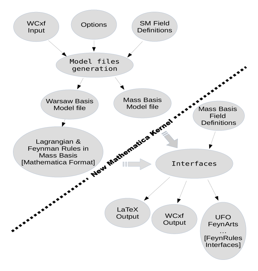
Figure 1: Structure of the SmeftFR code.

To speed up the calculations, SmeftFR can evaluate Feynman rules for a chosen subset of operators only, generating dynamically the proper FeynRules “model files”. The calculations are divided in two stages, as illustrated in flowchart of Fig. 1. First, the SMEFT Lagrangian is initialised in Warsaw basis and transformed to mass eigenstates basis analytically, truncating all terms of the order ${\cal O}(\frac{1}{\Lambda^{3}})$ and higher. To speed up the program, at this stage all flavour parameters are considered to be tensors with indices without assigned numerical values (they are “Internal” parameters in FeynRules notation). The resulting mass basis Lagrangian and Feynman rules written in Mathematica format are stored on disk. In the second stage, the previously generated output can be used together with new “model file”, this time containing numerical values of (“External”) parameters, to export mass basis SMEFT interactions in various commonly used external formats such as Latex, WCxf and standard FeynRules supported interfaces – UFO, FeynArts and others.

3.3 Model initialisation

Option Allowed values Description Operators default: all operators List with subset of SMEFT operators included in calculations. Gauge Unitary, Rxi Choice of gauge fixing conditions WCXFInitFile ”” Name of file with numerical values of Wilson coefficients in the WCxf format. If this option is not set or the file does not exist, all Wilson coefficients are set to $0$. MajoranaNeutrino False, True Neutrino fields are treated as Majorana spinors if $Q_{\nu\nu}$ is included in the operator list, massless Weyl spinors otherwise. Setting this option to True allows one to use Majorana spinors also in the massless case. Correct4Fermion False, True Corrects relative sign of some 4-fermion interactions, fixing results produced by FeynRules . WBFirstLetter ”c” Customizable first letter of Wilson coefficient names in Warsaw basis (default $c_{G},\ldots$). Can be used to avoid convention clashes when comparing with other SMEFT bases. MBFirstLetter ”C” Customizable first letter of Wilson coefficient names in mass basis (default $C_{G},\ldots$).

Table 4: The allowed options of SMEFTInitializeModel routine. If an option is not specified, the default value (marked above in boldface) is assumed.

In the first step, the relevant FeynRules model files must be generated. This is done by calling the function:

SMEFTInitializeModel[Option1 $\to$ Value1, Option2 $\to$ Value2, $\ldots$]

with the allowed options listed in Table 4.

Names of operators used in SmeftFR are derived from the subscript indices of operators listed in Tables 1 and 2, with obvious transcriptions of “tilde” symbol and Greek letters to Latin alphabet. By default, all possible 59+1+4 SMEFT ($d=6$) operator classes are included in calculations, which is equivalent to setting:

Operators $\to$ { "G", "Gtilde", "W", "Wtilde", "phi", "phiBox", "phiD", "phiW", "phiB", "phiWB", "phiWtilde", "phiBtilde", "phiWtildeB", "phiGtilde", "phiG", "ephi", "dphi", "uphi", "eW", "eB", "uG", "uW", "uB", "dG", "dW", "dB", "phil1", "phil3", "phie", "phiq1", "phiq3", "phiu", "phid", "phiud", "ll", "qq1", "qq3", "lq1", "lq3", "ee", "uu", "dd", "eu", "ed", "ud1", "ud8", "le", "lu", "ld", "qe", "qu1", "qu8", "qd1", "qd8", "ledq", "quqd1", "quqd8", "lequ1", "lequ3", "vv", "duq", "qqu", "qqq", "duu" }

To speed up the derivation of Feynman rules and to get more compact expressions, the user can restrict the list above to any preferred subset of operators.

SmeftFR is fully integrated with the WCxf standard. Apart from numerically editing Wilson coefficients in FeynRules model files, reading them from the WCxf input is the only way of automatic initialisation of their numerical values. Such an input format is exchangeable between a larger set of SMEFT-related public packages [21] and may help to compare their results.

An additional advantage of using WCxf input format comes in the flavour sector of the theory. Here, Wilson coefficients are in general tensors with flavour indices, in many cases symmetric under various permutations. WCxf input requires initialisation of only the minimal set of flavour dependent Wilson coefficients, those which could be derived by permutations are also automatically properly set.

Further comments concern MajoranaNeutrino and Correct4Fermion options. They are used to modify the analytical expressions only for the Feynman rules, not at the level of the mass basis Lagrangian from which the rules are derived. This is because some FeynRules interfaces, like UFO, intentionally leave the relative sign of 4-fermion interactions uncorrected, as it is later changed by Monte Carlo generators like MadGraph5. Correcting the sign before generating UFO output would therefore lead to wrong final result. Similarly, treatment of neutrinos as Majorana fields could not be compatible with hard coded quantum number definitions in various packages. On the other hand, in the manual or symbolic computations it is convenient to have from the start the correct form of Feynman rules, as done by SmeftFR when both options are set to their default values.

SMEFTInitializeModel routine does not require prior loading of FeynRules package. After execution, it creates in the output subdirectory three model files listed in Table 5. Parameter files generated by SMEFTInitializeModel contain also definitions of SM parameters, copied from templates definitions/smeft_par_head_WB.fr and definitions/smeft_par_head_MB.fr. The values of SM parameters can be best updated directly by editing the template files and the header of the code/smeft_variables.m file, otherwise they will be overwritten in each rerun of SmeftFR initialisation routines.

smeft_par_WB.par SMEFT parameter file with Wilson coefficients in Warsaw basis (defined as “Internal”, with no numerical values assigned). smeft_par_MB.par SMEFT parameter file with Wilson coefficients in mass basis (defined as “External”, numerical values imported from the input file in WCxf format). smeft_par_MB_real.par as smeft_par_MB.par, but only real values of Wilson coefficients given in WCxf file are included in SMEFT parameter file, as required by many event generators.

Table 5: Model files generated by the SMEFTInitializeModel routine.

As mentioned above, in all analytical calculations performed by SmeftFR , terms suppressed by ${\cal O}(1/\Lambda^{3})$ or higher $1/\Lambda$ powers are always neglected. Therefore, the resulting Feynman rules can be consistently used to calculate physical observables, symbolically or numerically by Monte Carlo generators, up to the linear order in dimension-6 operators. This information is encoded in FeynRules SMEFT model files by assigning the “interaction order” parameter NP=1 to each Wilson coefficients and setting in smeft_field_WB.fr and smeft_field_MB.fr the limits:

M$InteractionOrderLimit = {

{QCD,99},

{NP,1},

{QED,99}

}

If one wishes to include (e.g. for testing purposes) terms quadratic in Wilson coefficients in the automatic cross section calculations performed by matrix element and Monte Carlo generators, one should edit both model files and increase the allowed order of NP contributions by changing the definition of M$InteractionOrderLimit, setting there {NP,2}.

An additional remark concerns the value of neutrino masses. In mass basis, the neutrino masses are equal to $-v^{2}C_{\nu\nu}^{II}$  [see eq. (2.17)]. Thus, the numerical values of $C_{\nu\nu}^{II}$ coefficients should be real and negative. If positive or complex values of $C_{\nu\nu}^{II}$ are given in the WCxf input file, then the SMEFTInitializeModel routine evaluates neutrino masses as $M_{\nu^{I}}=v^{2}|C_{\nu\nu}^{II}|$.

3.4 Calculation of mass basis Lagrangian and Feynman rules

By loading the FeynRules model files the derivation of SMEFT Lagrangian in mass basis is performed by calling the following sequence of routines:

SMEFTLoadModel[ ]	Loads output/smeft_par_WB.par model file and calculates SMEFT Lagrangian in Warsaw basis for chosen subset of operators
SMEFTFindMassBasis[ ]	Finds field bilinears and analytical transformations diagonalizing mass matrices up to ${\cal O}(1/\Lambda^{2})$
SMEFTFeynmanRules[ ]	Evaluates analytically SMEFT Lagrangian and Feynman rules in the mass basis, again truncating consistently all terms higher then ${\cal O}(1/\Lambda^{2})$.

The calculation time may vary considerably depending on the choice of operator (sub-)set and gauge fixing conditions chosen. For the full list of SMEFT $d=5$ and $d=6$ operators and in $R_{\xi}$-gauges, one can expect CPU time necessary to evaluate all Feynman rules, from about an hour to many hours on a typical personal computer, depending on its speed capabilities.

One should note that when neutrinos are treated as Majorana particles, (as necessary in case of non-vanishing Wilson coefficient of $d=5$ Weinberg operator), their interactions involve lepton number non-conservation. When FeynRules is dealing with them it produces warnings of the form:

QN::NonConserv: Warning: non quantum number conserving vertex encountered!
Quantum number LeptonNumber not conserved in vertex $\ldots$

Obviously such warnings should be ignored.

Evaluation of Feynman rules for vertices involving more than two fermions is not fully implemented yet in FeynRules. To our experience, apart from the issue of relative sign of four fermion diagrams mentioned earlier, particularly problematic was the correct automatic derivation of quartic interactions with four Majorana neutrinos and similar vertices which violate $B$- and $L$-quantum numbers. For these special cases, SmeftFR overwrites the FeynRules result with manually calculated formulae encoded in Mathematica format.

Another remark concerns the hermicity property of the SMEFT Lagrangian. For some types of interactions, e.g. four-fermion vertices involving two-quarks and two-leptons, the function CheckHermicity provided by FeynRules reports non-Hermitian terms in the Lagrangian. However, such terms are actually Hermitian if permutation symmetries of indices of relevant Wilson coefficients are taken into account. Such symmetries are automatically imposed if numerical values of Wilson coefficients are initialized with the use of SMEFTInitializeMB or SMEFTToWCXF routines (see Sections 3.5 and 3.5.1).

Results of the calculations are collected in file output/smeft_feynman_rules.m. The Feynman rules and pieces of the mass basis Lagrangian for various classes of interactions are stored in the variables with self-explanatory names listed in Table 6.

LeptonGaugeVertices QuarkGaugeVertices LeptonHiggsGaugeVertices QuarkHiggsGaugeVertices QuarkGluonVertices GaugeSelfVertices GaugeHiggsVertices GluonSelfVertices GluonHiggsVertices GhostVertices FourLeptonVertices FourQuarkVertices TwoQuarkTwoLeptonVertices DeltaLTwoVertices BLViolatingVertices

Table 6: Names of variables defined in the file output/smeft_feynman_rules.m containing expressions for Feynman rules. Parts of mass basis Lagrangian are stored in equivalent set of variables, with “Vertices” replaced by “Lagrangian” in part of their names (i.e. LeptonGaugeVertices $\to$ LeptonGaugeLagrangian, etc.).

File output/smeft_feynman_rules.m contains also expressions for the normalisation factors relating Higgs and gauge fields and couplings in the Warsaw and mass basis. Namely, variables Hnorm, G0norm, GPnorm, AZnorm[i,j], Wnorm, Gnorm, correspond to, respectively, $Z_{h}^{-1}$, $Z_{G^{0}}^{-1}$, $Z_{G^{+}}^{-1}$ $\hat{Z}_{AZ}^{-1}$, $Z_{W}^{-1}$ and $Z_{G}^{-1}$ in (2.13). In addition, formulae for tree level corrections to SM mass parameters and Yukawa couplings are stored in variables SMEFT$vev, SMEFT$MH2, SMEFT$MW2, SMEFT$MZ2, SMEFT$YL[i,j], SMEFT$YD[i,j] and SMEFT$YU[i,j].

It is important to note that although at this point the Feynman rules for the mass basis Lagrangian are already calculated, definitions for fields and parameters used to initialise the SMEFT model in FeynRules are still given in Warsaw basis. To avoid inconsistencies, it is strongly advised to quit the current Mathematica kernel and start new one reloading the mass basis Lagrangian together with the compatible model files with fields defined also in mass basis, as described next in Sec. 3.5. All further calculations should be performed within this new kernel.

3.5 Interfaces

SmeftFR output in some of portable formats must be generated from the SMEFT Lagrangian transformed to mass basis, with all numerical values of parameters initialised. As FeynRules does not allow for two different model files loaded within a single Mathematica session, one needs to quit the kernel used to run routines necessary to obtain Feynman rules and, as described in previous Section, start a new Mathematica kernel. Within it, the user must reload FeynRules and SmeftFR packages and call the following routine:

SMEFTInitializeMB[ Options ]

Allowed options are given in Table 7. After call to SMEFTInitializeMB, mass basis model files are read and the mass basis Lagrangian is stored in a global variable named SMEFTMBLagrangian for further use by interface routines.

Option Allowed values Description RealParameters False, True Default initialisation is done using output/smeft_par_MB.par file, which may contain complex parameters, not compatible with matrix element generators. Setting RealParameters $\to$ True forces loading of output/smeft_par_MB_real.par file where imaginary parts of all Wilson coefficients are set to $0$. Imaginary phases of CKM and PMNS matrices, if present, are also set to zero after loading this file. Include4Fermion False, True 4-fermion vertices are not fully implemented in FeynRules and by default not included in SMEFT interactions. Set this option to True to include such terms.

Table 7: Options of SMEFTInitializeMB routine, with default values marked in boldface.

3.5.1 WCxf input and output

Translation between FeynRules model files and WCxf format is done by the functions SMEFTToWCXF and WCXFToSMEFT. They can be used standalone and do not require loading FeynRules and calling first SMEFTInitializeMB routine to work properly.

Exporting numerical values of Wilson coefficients of operators in the WCxf format is done by the function:

SMEFTToWCXF[ SMEFT_Parameter_File, WCXF_File ]

where the arguments SMEFT_Parameter_File, WCXF_File define the input model parameter file in the FeynRules format and the output file in the WCxf JSON format, respectively. The created JSON file can be used to transfer numerical values of Wilson coefficients to other codes supporting WCxf format. Note that in general, the FeynRules model files may contain different classes of parameters, according to the Value property defined to be a number (real or complex), a formula or even not defined at all. Only the Wilson coefficients with Value defined to be a number are transferred to the output file in WCxf format.

Conversely, files in WCxf format can be translated to FeynRules parameter files using:

WCXFToSMEFT[ WCXF_File, SMEFT_Parameter_File Options]

with the allowed options defined in Table 8.

Option Allowed values Description Operators default: all operators List with subset of Wilson coefficients to be included in the SMEFT parameter file RealParameters False, True Decides if only real values of Wilson coefficients given in WCxf file are included in SMEFT parameter file OverwriteTarget False, True If set to True, target file is overwritten without warning Silent False, True Debug option, suppresses screen comments FirstLetter ”C” Customizable first letter of Wilson coefficient names in mass basis (default $C_{G},\ldots$).

Table 8: Options of WCXFToSMEFT routine. Default values are marked in boldface.

3.5.2 Latex output

SmeftFR provides a dedicated Latex generator (not using the generic FeynRules Latex export routine). Its output has the following structure:

• For each interaction vertex, the diagram is drawn, using the axodraw style [46]. Expressions for Feynman rules are displayed next to corresponding diagrams.

• In analytical expressions, all terms multiplying a given Wilson coefficient are collected together and simplified.

• Long analytical expressions are automatically broken into many lines using breakn style (this does not always work perfectly but the printout is sufficiently readable).

Latex output is generated by the function:

SMEFTToLatex[ Options ]

with the allowed options listed in Table 9. The function SMEFTToLatex assumes that the variables listed in Table 6 are initialised. It can be called either after executing relevant commands, described in Sec. 3.4, or after reloading the mass basis Lagrangian with the SMEFTInitializeMB routine, see Sec. 3.5.

Option name Allowed values Description FullDocument False, True By default a complete document is generated, with all headers necessary for compilation. If set to False, headers are stripped off and the output file can, without modifications, be included into other Latex documents. ScreenOutput False, True For debugging purposes, if set to True the Latex output is printed also to the screen.

Table 9: Options of SMEFTToLatex routine, with default values marked in boldface.

Latex output is stored in output/latex subdirectory, split into smaller files each containing one primary vertex. The main file is named smeft_feynman_rules.tex. The style files necessary to compile Latex output are supplied with the SmeftFR distribution.

Note that the correct compilation of documents using “axodraw.sty” style requires creating intermediate Postscript file. Programs like pdflatex producing directly PDF output will not work properly. One should instead use e.g.:

latex smeft_feynman_rules.tex

dvips smeft_feynman_rules.dvi

ps2pdf smeft_feynman_rules.ps

The smeft_feynman_rules.tex does not contain analytical expressions for five and six gluon vertices. Such formulae are very long (multiple pages, hard to even compile properly) and not useful for hand-made calculations. If such vertices are needed, they should be rather directly exported in some other formats as described in the next subsection.

Other details not printed in the Latex output, such as, the form of field propagators, conventions for parameters and momenta flow in vertices (always incoming), manipulation of four-fermion vertices with Majorana fermions etc, are explained thoroughly in the Appendices A1–A3 of ref. [10].

3.5.3 Standard FeynRules interfaces

After calling the initialisation routine SMEFTInitializeMB, the output to UFO, FeynArts and other formats supported by FeynRules interfaces, can be generated using FeynRules commands and options from the mass basis Lagrangian stored in the SMEFTMBLagrangian variable. For instance, one could call:

WriteUFO[ SMEFTMBLagrangian, Output $\to$ ”output/UFO”, AddDecays $\to$ False, …]

WriteFeynArtsOutput[ SMEFTMBLagrangian, Output $\to$ ”output/FeynArts”, …]

and similarly for other formats.

It is important to note that FeynRules interfaces like UFO or FeynArts generate their output starting from the level of SMEFT mass basis Lagrangian. Thus, options of SMEFTInitializeModel function like MajoranaNeutrino and Correct4Fermion (see Table 4) have no effect on output generated by the interface routines. As explained in Section 3.3 they affect only the expressions for Feynman rules.

If four-fermion vertices are included in SMEFT Lagrangian, UFO produces warning messages of the form:

Warning: Multi-Fermion operators are not yet fully supported!

Therefore, the output for four-fermion interactions in UFO or other formats must be treated with care and limited trust — performing appropriate checks are left to users’ responsibility. To our experience, implementation in FeynRules of baryon and lepton number violating four-fermion interactions, with charge conjugation matrix appearing explicitly in vertices, is even more problematic. Thus, for safety in current SmeftFR version (2.00) such terms are never included in SMEFTMBLagrangian variable, eventually they can be passed to interface routines separately via the BLViolatingLagrangian variable.

Exporting to UFO or other formats can take a long time, even several hours for $R_{\xi}$-gauges and complete SMEFT Lagrangian with fully general flavour structure and all numerical values of parameters initialised.

Finally, it is important to stress here that our Feynman rules communicate properly with MadGraph5 and FeynArts. In particular, we ran without errors test simulations in MadGraph5 using UFO model files produced by SmeftFR v2. Similar tests were performed with amplitude generation for sample processes using SmeftFR v2 FeynArts output.

4 Sample programs

After setting the variable $FeynRulesPath to correct value, in order to evaluate mass basis SMEFT Lagrangian and analytical form of Feynman rules one can use the following sequence of commands:

SMEFT$MajorVersion = "2";
SMEFT$MinorVersion = "00";
SMEFT$Path = FileNameJoin[{$FeynRulesPath, "Models", "SMEFT_" <>
                                    SMEFT$MajorVersion <> "_" <> SMEFT$MinorVersion}];

Get[ FileNameJoin[$FeynRulesPath,"FeynRules.m"] ];
Get[ FileNameJoin[ SMEFT$Path, "code", "smeft_package.m"] ];

OpList = { "G", "Gtilde", "W", "Wtilde", "phi", "phiBox", "phiD", "phiW", "phiB", "phiWB", "phiWtilde", "phiBtilde", "phiWtildeB", "phiGtilde", "phiG", "ephi", "dphi", "uphi", "eW", "eB", "uG", "uW", "uB", "dG", "dW", "dB", "phil1", "phil3", "phie", "phiq1", "phiq3", "phiu", "phid", "phiud", "ll", "qq1", "qq3", "lq1", "lq3", "ee", "uu", "dd", "eu", "ed", "ud1", "ud8", "le", "lu", "ld", "qe", "qu1", "qu8", "qd1", "qd8", "ledq", "quqd1", "quqd8", "lequ1", "lequ3", "vv", "duq", "qqu", "qqq", "duu" };

SMEFTInitializeModel[ Operators -> OpList, Gauge -> Rxi, WCXFInitFile -> "wcxf_input_file_with_path.json" ];

SMEFTLoadModel[ ];
SMEFTFindMassBasis[ ];
SMEFTFeynmanRules[ ];

or alternatively rerun the supplied programs: the notebook SmeftFR-init.nb or the text script smeft_fr_init.m.

As described before, Latex, WCxf, UFO and FeynArts formats can be exported after rerunning first SmeftFR-init.nb or equivalent set of commands generating file smeft_feynman_rules.m containing the expressions for the mass basis Lagrangian. Then, the user needs to start a new Mathematica kernel and rerun the notebook file SmeftFR-interfaces.nb or the script smeft_fr_interfaces.m. Alternatively, one can manually type the commands, if necessary changing some of their options as described in previous sections:

Get[ FileNameJoin[{$FeynRulesPath,"FeynRules.m"}] ];
Get[ FileNameJoin[{SMEFT$Path, "code", "smeft_package.m"}] ];

SMEFTInitializeMB[ ];

SMEFTToWCXF[ FileNameJoin[{SMEFT$Path, "output", "smeft_par_MB.fr"}],
                        FileNameJoin[{SMEFT$Path, "output", "smeft_wcxf_MB.json"}] ];
SMEFToLatex[ ];

WriteUFO[ SMEFTMBLagrangian, $\ldots$ ];
WriteFeynArtsOutput[ SMEFTMBLagrangian, $\ldots$ ];

Feynman rules calculated for the full SMEFT operator set and two possible gauge choices (unitary and $R_{\xi}$), including also outputs in Latex, UFO and FeynArts formats, are stored in the subdirectories full_rxi_results and full_unitary_results. They can be directly used, without rerunning the SmeftFR package. However, such a general output with all operators and numerical values for all 2499 SMEFT parameters initialised, is huge and importing it directly to other SMEFT codes may cause them to work very slowly.

5 Summary

The proliferation of the primitive vertices in SMEFT, even in non-redundant basis of effective field operators, suggests a certain kind of computational aid. During the last few years, such an effort has been intensive between high energy physicists. Aiming at this direction, we present here a code, named SmeftFR, that generates Feynman rules in SMEFT with $\text{dimension}\leq 6$ operators given in “Warsaw basis” [9] without restricting to specific flavour structure, $CP$-, $B$- nor $L$-number conservation. We have exploited the quantisation steps of SMEFT in unitary and $R_{\xi}$-gauges following a procedure described in ref. [10]. SmeftFR has been written on top of the Mathematica package FeynRules.

In this article, we describe how to use SmeftFR package in order to produce Feynman rules for a selection of operators relevant to observable (or observables) under study, with further options to handle massive Majorana or massless Weyl neutrinos. The output of the package can be printed in Latex or exported in various formats supported by FeynRules, such as UFO, FeynArts, etc. Input parameters for Wilson coefficients used in SmeftFR can communicate with WCxf format for further numerical handling. Feynman rules are given in SMEFT mass basis and in both unitary or linear $R_{\xi}$-gauges for further computational checks.

The current version of SmeftFR code and its manual can be downloaded from the address

www.fuw.edu.pl/smeft

We believe that SmeftFR is bridging a gap between the effective SM Lagrangian all the way down to amplitude calculations required by the experimental analyses.

References

- [1] A. Dedes, W. Materkowska, M. Paraskevas, J. Rosiek and K. Suxho, “Feynman rules for the Standard Model Effective Field Theory in Rξ-gauges,” JHEP 1706, 143 (2017), arXiv:1704.03888.
- [2] A. Alloul, N. D. Christensen, C. Degrande, C. Duhr and B. Fuks, “FeynRules 2.0 - A complete toolbox for tree-level phenomenology,” Comput. Phys. Commun. 185, 2250 (2014), arXiv:1310.1921.

References

- [1] S. Weinberg, A Model of Leptons, Phys.Rev.Lett. 19 (1967) 1264–1266. doi:10.1103/PhysRevLett.19.1264.
- [2] S. Glashow, Partial Symmetries of Weak Interactions, Nucl.Phys. 22 (1961) 579–588. doi:10.1016/0029-5582(61)90469-2.
- [3] A. SalamIn Proceedings of the Eighth Nobel Symposium, edited by N. Svartholm (Wiley, New York, 1968), p.367.
- [4] S. Weinberg, Effective Gauge Theories, Phys. Lett. B91 (1980) 51–55. doi:10.1016/0370-2693(80)90660-7.
- [5] S. R. Coleman, J. Wess, B. Zumino, Structure of phenomenological Lagrangians. 1., Phys. Rev. 177 (1969) 2239–2247. doi:10.1103/PhysRev.177.2239.
- [6] C. G. Callan, Jr., S. R. Coleman, J. Wess, B. Zumino, Structure of phenomenological Lagrangians. 2., Phys. Rev. 177 (1969) 2247–2250. doi:10.1103/PhysRev.177.2247.
- [7] A. V. Manohar, Introduction to Effective Field Theories, in: Les Houches summer school: EFT in Particle Physics and Cosmology Les Houches, Chamonix Valley, France, July 3-28, 2017, 2018. arXiv:1804.05863.
- [8] W. Buchmuller, D. Wyler, Effective Lagrangian Analysis of New Interactions and Flavor Conservation, Nucl. Phys. B268 (1986) 621–653. doi:10.1016/0550-3213(86)90262-2.
- [9] B. Grzadkowski, M. Iskrzynski, M. Misiak, J. Rosiek, Dimension-Six Terms in the Standard Model Lagrangian, JHEP 10 (2010) 085. arXiv:1008.4884, doi:10.1007/JHEP10(2010)085.
- [10] A. Dedes, W. Materkowska, M. Paraskevas, J. Rosiek, K. Suxho, Feynman rules for the Standard Model Effective Field Theory in Rξ -gauges, JHEP 06 (2017) 143. arXiv:1704.03888, doi:10.1007/JHEP06(2017)143.
- [11] A. Alloul, N. D. Christensen, C. Degrande, C. Duhr, B. Fuks, FeynRules 2.0 - A complete toolbox for tree-level phenomenology, Comput. Phys. Commun. 185 (2014) 2250–2300. arXiv:1310.1921, doi:10.1016/j.cpc.2014.04.012.
- [12] C. Degrande, C. Duhr, B. Fuks, D. Grellscheid, O. Mattelaer, T. Reiter, UFO - The Universal FeynRules Output, Comput. Phys. Commun. 183 (2012) 1201–1214. arXiv:1108.2040, doi:10.1016/j.cpc.2012.01.022.
- [13] J. Alwall, R. Frederix, S. Frixione, V. Hirschi, F. Maltoni, O. Mattelaer, H. S. Shao, T. Stelzer, P. Torrielli, M. Zaro, The automated computation of tree-level and next-to-leading order differential cross sections, and their matching to parton shower simulations, JHEP 07 (2014) 079. arXiv:1405.0301, doi:10.1007/JHEP07(2014)079.
- [14] T. Gleisberg, S. Hoeche, F. Krauss, M. Schonherr, S. Schumann, F. Siegert, J. Winter, Event generation with SHERPA 1.1, JHEP 02 (2009) 007. arXiv:0811.4622, doi:10.1088/1126-6708/2009/02/007.
- [15] A. Belyaev, N. D. Christensen, A. Pukhov, CalcHEP 3.4 for collider physics within and beyond the Standard Model, Comput. Phys. Commun. 184 (2013) 1729–1769. arXiv:1207.6082, doi:10.1016/j.cpc.2013.01.014.
- [16] W. Kilian, T. Ohl, J. Reuter, WHIZARD: Simulating Multi-Particle Processes at LHC and ILC, Eur. Phys. J. C71 (2011) 1742. arXiv:0708.4233, doi:10.1140/epjc/s10052-011-1742-y.
- [17] N. D. Christensen, C. Duhr, B. Fuks, J. Reuter, C. Speckner, Introducing an interface between WHIZARD and FeynRules, Eur. Phys. J. C72 (2012) 1990. arXiv:1010.3251, doi:10.1140/epjc/s10052-012-1990-5.
- [18] T. Hahn, Generating Feynman diagrams and amplitudes with FeynArts 3, Comput. Phys. Commun. 140 (2001) 418–431. arXiv:hep-ph/0012260, doi:10.1016/S0010-4655(01)00290-9.
- [19] V. Shtabovenko, R. Mertig, F. Orellana, New Developments in FeynCalc 9.0, Comput. Phys. Commun. 207 (2016) 432–444. arXiv:1601.01167, doi:10.1016/j.cpc.2016.06.008.
- [20] T. Hahn, Feynman Diagram Calculations with FeynArts, FormCalc, and LoopTools, PoS ACAT2010 (2010) 078. arXiv:1006.2231, doi:10.22323/1.093.0078.
- [21] J. Aebischer, et al., WCxf: an exchange format for Wilson coefficients beyond the Standard Model, Comput. Phys. Commun. 232 (2018) 71–83. arXiv:1712.05298, doi:10.1016/j.cpc.2018.05.022.
- [22] A. Dedes, M. Paraskevas, J. Rosiek, K. Suxho, L. Trifyllis, The decay in the Standard-Model Effective Field Theory, JHEP 08 (2018) 103. arXiv:1805.00302, doi:10.1007/JHEP08(2018)103.
- [23] A. Dedes, K. Suxho, L. Trifyllis, The decay in the Standard-Model Effective Field TheoryarXiv:1903.12046.
- [24] S. Dawson, P. P. Giardino, Higgs decays to and in the standard model effective field theory: An NLO analysis, Phys. Rev. D97 (9) (2018) 093003. arXiv:1801.01136, doi:10.1103/PhysRevD.97.093003.
- [25] E. Vryonidou, C. Zhang, Dimension-six electroweak top-loop effects in Higgs production and decay, JHEP 08 (2018) 036. arXiv:1804.09766, doi:10.1007/JHEP08(2018)036.
- [26] H. Hesari, H. Khanpour, M. Mohammadi Najafabadi, Study of Higgs Effective Couplings at Electron-Proton Colliders, Phys. Rev. D97 (9) (2018) 095041. arXiv:1805.04697, doi:10.1103/PhysRevD.97.095041.
- [27] S. Dawson, P. P. Giardino, Electroweak corrections to Higgs boson decays to and in standard model EFT, Phys. Rev. D98 (9) (2018) 095005. arXiv:1807.11504, doi:10.1103/PhysRevD.98.095005.
- [28] S. Dawson, A. Ismail, Standard model EFT corrections to Z boson decays, Phys. Rev. D98 (9) (2018) 093003. arXiv:1808.05948, doi:10.1103/PhysRevD.98.093003.
- [29] J. Baglio, S. Dawson, I. M. Lewis, NLO Effects in EFT Fits to Production at the LHC, Phys. Rev. D99 (3) (2019) 035029. arXiv:1812.00214, doi:10.1103/PhysRevD.99.035029.
- [30] S. Dawson, P. P. Giardino, A. Ismail, SMEFT and the Drell-Yan Process at High EnergyarXiv:1811.12260.
- [31] L. Silvestrini, M. Valli, Model-independent Bounds on the Standard Model Effective Theory from Flavour PhysicsarXiv:1812.10913.
- [32] T. Neumann, Z. E. Sullivan, Off-shell single-top-quark production in the Standard Model Effective Field TheoryarXiv:1903.11023.
- [33] J. Aebischer, J. Kumar, D. M. Straub, Wilson: a Python package for the running and matching of Wilson coefficients above and below the electroweak scale, Eur. Phys. J. C78 (12) (2018) 1026. arXiv:1804.05033, doi:10.1140/epjc/s10052-018-6492-7.
- [34] A. Celis, J. Fuentes-Martin, A. Vicente, J. Virto, DsixTools: The Standard Model Effective Field Theory Toolkit, Eur. Phys. J. C77 (6) (2017) 405. arXiv:1704.04504, doi:10.1140/epjc/s10052-017-4967-6.
- [35] J. C. Criado, MatchingTools: a Python library for symbolic effective field theory calculations, Comput. Phys. Commun. 227 (2018) 42–50. arXiv:1710.06445, doi:10.1016/j.cpc.2018.02.016.
- [36] I. Brivio, Y. Jiang, M. Trott, The SMEFTsim package, theory and tools, JHEP 12 (2017) 070. arXiv:1709.06492.
- [37] S. Das Bakshi, J. Chakrabortty, S. K. Patra, CoDEx: Wilson coefficient calculator connecting SMEFT to UV theory, Eur. Phys. J. C79 (1) (2019) 21. arXiv:1808.04403, doi:10.1140/epjc/s10052-018-6444-2.
- [38] M. Gabelmann, M. Mühlleitner, F. Staub, Automatised matching between two scalar sectors at the one-loop level, Eur. Phys. J. C79 (2) (2019) 163. arXiv:1810.12326, doi:10.1140/epjc/s10052-019-6570-5.
- [39] F. Bishara, J. Brod, B. Grinstein, J. Zupan, DirectDM: a tool for dark matter direct detectionarXiv:1708.02678.
- [40] A. Denner, H. Eck, O. Hahn, J. Kublbeck, Feynman rules for fermion number violating interactions, Nucl. Phys. B387 (1992) 467–481. doi:10.1016/0550-3213(92)90169-C.
- [41] A. Denner, H. Eck, O. Hahn, J. Kublbeck, Compact Feynman rules for Majorana fermions, Phys. Lett. B291 (1992) 278–280. doi:10.1016/0370-2693(92)91045-B.
- [42] M. Paraskevas, Dirac and Majorana Feynman Rules with four-fermionsarXiv:1802.02657.
- [43] E. E. Jenkins, A. V. Manohar, M. Trott, Renormalization Group Evolution of the Standard Model Dimension Six Operators I: Formalism and lambda Dependence, JHEP 10 (2013) 087. arXiv:1308.2627, doi:10.1007/JHEP10(2013)087.
- [44] E. E. Jenkins, A. V. Manohar, M. Trott, Renormalization Group Evolution of the Standard Model Dimension Six Operators II: Yukawa Dependence, JHEP 01 (2014) 035. arXiv:1310.4838, doi:10.1007/JHEP01(2014)035.
- [45] R. Alonso, E. E. Jenkins, A. V. Manohar, M. Trott, Renormalization Group Evolution of the Standard Model Dimension Six Operators III: Gauge Coupling Dependence and Phenomenology, JHEP 04 (2014) 159. arXiv:1312.2014, doi:10.1007/JHEP04(2014)159.
- [46] J. A. M. Vermaseren, Axodraw, Comput. Phys. Commun. 83 (1994) 45–58. doi:10.1016/0010-4655(94)90034-5.