The leading hadronic contribution to $(g-2)_{\mu}$ from lattice QCD with $N_{\rm f}=2+1$ flavours of O($a$) improved Wilson quarks

Abstract

The comparison of the theoretical and experimental determinations of the anomalous magnetic moment of the muon $(g-2)_{\mu}$ constitutes one of the strongest tests of the Standard Model at low energies. In this article, we compute the leading hadronic contribution to $(g-2)_{\mu}$ using lattice QCD simulations employing Wilson quarks. Gauge field ensembles at four different lattice spacings and several values of the pion mass down to its physical value are used. We apply the O($a$) improvement programme with two discretizations of the vector current to better constrain the approach to the continuum limit. The electromagnetic current correlators are computed in the time-momentum representation. In addition, we perform auxiliary calculations of the pion form factor at timelike momenta in order to better constrain the tail of the isovector correlator and to correct its dominant finite-size effect. For the numerically dominant light-quark contribution, we have rescaled the lepton mass by the pion decay constant computed on each lattice ensemble. We perform a combined chiral and continuum extrapolation to the physical point, and our final result is $a_{\mu}^{\rm hvp}=(720.0\pm 12.4_{\rm stat}\,\pm 9.9_{\rm syst})\cdot 10^{-10}$. It contains the contributions of quark-disconnected diagrams, and the systematic error has been enlarged to account for the missing isospin-breaking effects.

I Introduction

Electrons and muons carry a magnetic moment, which is correctly predicted by Dirac’s original theory of the electron to within a permille of precision. The proportionality factor between the spin and the magnetic moment of the lepton $\ell$ is parameterized by the gyromagnetic ratio $g$. In Dirac’s theory, $g=2$, and one characterizes the deviation of $g$ from this reference value by $a_{\ell}=(g-2)_{\ell}/2$. Testing the ability of Quantum Electrodynamics (QED) to correctly predict this precision observable has played a crucial role in the development of quantum field theory in general. Presently, the achieved experimental precision of 540 ppb on the measurement of the anomalous magnetic moment of the muon Bennett et al. (2006), $a_{\mu}$, requires the effects of all three interactions of the Standard Model (SM) of particle physics to be included in the theory prediction. In fact, a tension of about 3.5 standard deviations exists between the SM prediction and the experimental measurement. For reviews on the subject, we refer the reader to Jegerlehner and Nyffeler (2009); Blum et al. (2013); Jegerlehner (2017).

Presently, the E989 experiment at Fermilab is performing a new direct measurement of $a_{\mu}$ Grange et al. (2015), and a further experiment using a different experimental technique is planned at J-PARC Mibe (2011). The final goal of these experiments is to reduce the uncertainty on $a_{\mu}$ by a factor of four. A reduction of the theory error is thus of paramount importance, as the first results from the Fermilab experiment are expected within the next few months. These will likely reach the same precision as the current world average.

On the theory side, the precision of the SM prediction for $a_{\mu}$ is completely dominated by hadronic uncertainties. The leading hadronic contribution enters at second order in the fine-structure constant $\alpha$ via the vacuum polarization and must be determined at the few-permille level in order to match the upcoming precision of the direct measurements of $a_{\mu}$. In this paper we undertake a first-principles lattice QCD calculation of this hadronic contribution (see Meyer and Wittig (2019) for a recent review of previous lattice results). A further hadronic effect, the light-by-light scattering contribution which enters at third order in the fine-structure constant, currently contributes at a comparable level to the theory uncertainty budget and is being addressed both by dispersive and lattice methods (see Blum et al. (2017); Asmussen et al. (2018); Colangelo et al. (2018) and references therein).

Our calculation of the hadronic vacuum polarization to the anomalous magnetic moment of the muon, $a_{\mu}^{\rm hvp}$, fully includes the effects of the up, down and strange quarks, while the charm quark (whose contribution to $a_{\mu}^{\rm hvp}$ is small) is treated only at the valence level. We use ensembles of SU(3) gauge field configurations generated with an O($a$) improved Wilson quark action as part of the Coordinated Lattice Simulations (CLS) initiative Bruno et al. (2015); Bali et al. (2016a). In particular, the generation of a physical-mass ensemble Mohler et al. (2018) (labelled E250) was largely motivated by the goal of improving the lattice determination of $a_{\mu}^{\rm hvp}$. We use four different lattice spacings to control the continuum limit, and the $(u,d,s)$ quark masses are varied at constant average quark mass in order to perform a chiral interpolation to the physical values of the quark masses Bruno et al. (2015). Our calculation is performed at equal up and down quark masses, and no QED effects are included; however, in the future both of these isospin-breaking effects will be taken into account as corrections Risch and Wittig (2018a, b).

Lattice QCD, which is formulated in Euclidean space, is well suited for computing $a_{\mu}^{\rm hvp}$, since the latter only involves the two-point function of the hadronic component of the electromagnetic current at spacelike momenta Blum (2003). In this work we employ the representation of $a_{\mu}^{\rm hvp}$ as a Euclidean-time integral over the two-point function in the time-momentum representation (TMR) Bernecker and Meyer (2011), i.e. projected to vanishing spatial momentum. This representation does not require a parameterization of the vacuum polarization function and has a clear spectral interpretation in terms of vector hadronic states in the center-of-mass frame. The main difficulty in obtaining $a_{\mu}^{\rm hvp}$ with good statistical precision is that it probes the TMR correlator at Euclidean times well beyond 2 fm, where its relative precision deteriorates rapidly. Therefore a dedicated treatment of the tail of the correlator which does not compromise the first-principles nature of the calculation is needed. Here the spectral representation of the correlator plays a central role.

An important source of systematic uncertainty is the correction to $a_{\mu}^{\rm hvp}$ due to the use of a finite spatial torus. On our lattice ensembles, this finite-size effect (FSE) mostly stems from the tail of the isovector component of the TMR correlator. Thanks to precise relations Lüscher (1991); Meyer (2011) between the properties of the discrete quantum states on the torus and the pion form factor at timelike momenta, we are able to correct for the dominant part of the FSE. Finally, the quark-disconnected diagrams, while making only a few-percent contribution to $a_{\mu}^{\rm hvp}$, require a dedicated set of calculations for their evaluation, which demand a large computing-time investment.

The rest of this paper is organized as follows. Section II describes the methodology followed in our calculation, including the renormalization and improvement of the TMR correlator and the treatment of the charm contribution. Section III presents our lattice data and the extraction of the observable $a_{\mu}^{\rm hvp}$ on each individual lattice ensemble. In section IV, the lattice-spacing and quark-mass dependence of these intermediate results is fitted in order to arrive at our final result. Finally, we compare the latter with phenomenological as well as other recent lattice determinations in section V.

II Methodology

II.1 Time-momentum correlators

We start by providing all relevant relations in the continuum and infinite-volume Euclidean theory. In the time-momentum representation (TMR), the leading-order hadronic vacuum polarization contribution to $(g-2)_{\mu}$ is given by the convolution integral

$$a_{\mu}^{\rm hvp}=\left(\frac{\alpha}{\pi}\right)^{2}\int_{0}^{\infty}\,dt\,\widetilde{K}(t)G(t),$$ (1)

where an analytic expression for the QED kernel function $\widetilde{K}(t)$ is given in Appendix B of Ref. Della Morte et al. (2017), and

$$G(t)\,\delta_{kl}=-\int d^{3}x\,\Big{\langle}J_{k}(t,\boldsymbol{x})\;J_{l}(0)\Big{\rangle}$$ (2)

is the spatially summed QCD two-point function of the electromagnetic current $\boldsymbol{J}=\frac{2}{3}\bar{u}\boldsymbol{\gamma}u-\frac{1}{3}\bar{d}\boldsymbol{\gamma}d-\frac{1}{3}\bar{s}\boldsymbol{\gamma}s+\frac{2}{3}\bar{c}\boldsymbol{\gamma}c$. In isospin-symmetric QCD, we can write

$$G(t)=\frac{5}{9}G_{l}(t)+\frac{1}{9}G_{s}(t)+\frac{4}{9}G_{c}(t)+G_{\rm disc}(t),$$ (3)

where $G_{f}(t)$ denotes a quark-connected contribution associated with flavour $f$ and $G_{\rm disc}(t)$ is the quark-disconnected contribution. An alternative decomposition based on the isospin quantum number $I$ yields

$$G(t)=G^{I=1}(t)+G^{I=0}(t),\qquad G^{I=1}(t)=\frac{1}{2}G_{l}(t).$$ (4)

Physically, the latter decomposition is more transparent. In particular, at light pion masses the dominant finite-size effects, as well as a logarithmic singularity as $m_{\pi}\to 0$, only concern the isovector contribution, $a_{\mu}^{{\rm hvp},I=1}$. Computationally however, the disconnected contributions are obtained very differently from the connected ones: they are costly and amount only to a few percent of the total. Therefore, in our numerical analysis there is an interesting interplay between the two choices of bases to compute $a_{\mu}^{\rm hvp}$.

With $m_{\mu}$ the muon mass, the kernel behaves as $\widetilde{K}(t)\sim\frac{\pi^{2}}{9}m_{\mu}^{2}t^{4}$ for $t\ll m_{\mu}^{-1}$ and as $\widetilde{K}(t)\sim 2\pi^{2}t^{2}$ for $t\gg m_{\mu}^{-1}$. Since the lattice data for the correlator $G(t)$ is in lattice units, the muon mass must be known in those units, $am_{\mu}$. The knowledge of the lattice spacing in $\mathrm{GeV}^{-1}$ thus plays a crucial role in a precision determination of $a_{\mu}^{\rm hvp}$ Della Morte et al. (2017, 2018). There are then two ways to proceed. In lattice QCD, where often the physical quark masses are reached only after an extrapolation or interpolation, $a_{\mu}^{\rm hvp}$ can either be calculated using the fixed, physical value of $m_{\mu}=105.66\,\mathrm{MeV}$; or the muon mass can be rescaled by a quantity with dimension of mass known experimentally Feng et al. (2011). In our calculation, we have explored both paths. In our final results, we adopt the “rescaling strategy” for the connected light contribution. As a rescaling quantity, we choose the pion decay constant $f_{\pi}$, so that we set

$$am_{\mu}=\Big{(}\frac{m_{\mu}}{f_{\pi}}\Big{)}_{\rm pheno}\cdot(af_{\pi})_{\rm lattice}=1.144\cdot(af_{\pi})_{\rm lattice}$$ (5)

on every lattice ensemble. Our choice is motivated, first, by $f_{\pi}$ being determined precisely and reliably, both in phenomenology and on the lattice; and secondly, since $f_{\pi}$ increases with the pion mass, this choice has the effect of making the $m_{\pi}$ dependence of $a_{\mu}^{\rm hvp}$ weaker. To intuitively understand the effect of the rescaling, it is instructive to consider the calculation of the anomalous magnetic moment of the electron; in this case, obtaining $a_{e}^{\rm hvp}=({4\alpha^{2}}/{3})m_{e}^{2}\Pi_{1}$ requires computing the time moment $\Pi_{1}\equiv({1}/{12})\int_{0}^{\infty}dt\;t^{4}\,G(t)$. Thus the rescaling simply amounts to computing the dimensionless quantity $f_{\pi}^{2}\Pi_{1}$, and converting the result into $a_{e}^{\rm hvp}$ by using the phenomenological value of $(m_{e}^{2}/f_{\pi}^{2})$.

II.2 Simulation parameters

Table 1: Parameters of the simulations: $\beta=6/g_{0}^{2}$ is the bare gauge coupling, $\kappa_{l,s}$ are the hopping parameters of the light and strange quarks, $a$ is the lattice spacing and $(L,T)$ are the lattice dimensions in space and time. Ensembles E250 and B450 have periodic boundary conditions in time, all others have open boundary conditions. The last column contains the number of gauge configurations used. Ensembles with an asterisk are not included in the final analysis but are used to control finite-size effects.

id	$\quad\beta\quad$	$L^{3}\times T$	$a\,[{\rm{fm}}]$	$~{}~{}~{}\kappa_{l}$	$~{}~{}~{}\kappa_{s}$	$m_{\pi}\,[\mathrm{MeV}]$	$m_{K}\,[\mathrm{MeV}]$	$m_{\pi}L$	$L\,[{\rm{fm}}]$	conf.
H101	3.40	$32^{3}\times 96$	0.08636	0.136760	0.136760	416(5)	416(5)	5.8	2.8	2000
H102		$32^{3}\times 96$		0.136865	0.13654934	354(5)	438(4)	5.0	2.8	1900
H105∗		$32^{3}\times 96$		0.136970	0.13634079	284(4)	460(4)	3.9	2.8	2800
N101		$48^{3}\times 128$		0.136970	0.13634079	282(4)	460(4)	5.9	4.1	1500
C101		$48^{3}\times 96$		0.137030	0.13622204	221(2)	472(8)	4.7	4.1	2600
B450	3.46	$32^{3}\times 64$	0.07634	0.136890	0.136890	416(4)	416(4)	5.2	2.4	1500
S400		$32^{3}\times 96$		0.136984	0.13670239	351(4)	438(5)	4.3	2.4	2800
N401		$48^{3}\times 128$		0.137062	0.13654808	287(4)	462(5)	5.3	3.7	1100
H200∗	3.55	$32^{3}\times 96$	0.06426	0.137000	0.137000	419(5)	419(5)	4.4	2.1	2000
N202		$48^{3}\times 128$		0.137000	0.137000	410(5)	410(5)	6.4	3.1	900
N203		$48^{3}\times 128$		0.137080	0.13684028	345(4)	441(5)	5.4	3.1	1500
N200		$48^{3}\times 128$		0.137140	0.13672086	282(3)	463(5)	4.4	3.1	1700
D200		$64^{3}\times 128$		0.137200	0.13660175	200(2)	480(5)	4.2	4.1	2000
E250		$96^{3}\times 192$		0.137233	0.13653663	130(1)		4.1	6.2	500
N300	3.70	$48^{3}\times 128$	0.04981	0.137000	0.137000	421(4)	421(4)	5.1	2.4	1700
N302		$48^{3}\times 128$		0.137064	0.13687218	346(4)	458(5)	4.2	2.4	2200
J303		$64^{3}\times 192$		0.137123	0.13675466	257(3)	476(5)	4.2	3.2	600

Our work is based on a subset of the Coordinated Lattice Simulations (CLS) ensembles with $N_{\rm f}=2+1$ dynamical quarks. They are generated Bruno et al. (2015) using the open-QCD suite Lüscher and Schaefer (2013) and are based on the O($a$)-improved Wilson-Clover action for fermions, with the parameter $c_{\rm sw}$ determined non perturbatively in Ref. Bulava and Schaefer (2013), and the tree-level O($a^{2}$) improved Lüscher-Weisz gauge action. The ensembles used in this analysis were generated at a constant value of the average bare quark mass such that the improved bare coupling $\tilde{g}_{0}$ is kept constant along the chiral trajectory Bruno et al. (2015). In particular, five of the ensembles are at the SU(3)-symmetric point, $m_{u}=m_{d}=m_{s}$. The parameters of the simulations are summarized in Table 1.

Results are obtained at four values of the lattice spacing in the range $a=0.050-0.086$ fm. The scale setting was performed in Ref. Bruno et al. (2017) using a linear combination of the pion and kaon decay constants with a precision of 1%. The pion masses used in our determination of $a_{\mu}^{\rm hvp}$ lie in the range $m_{\pi}\approx 130-420$ MeV. All the ensembles included in the final analysis satisfy $m_{\pi}L>4$. Furthermore, at two values of the pion mass ($m_{\pi}=280$ and 420 MeV), two ensembles with the same bare lattice parameters but different volumes are used to study finite-size effects. These ensembles with smaller volumes are not included in the final analysis and are marked by an asterisk in Table 1.

All ensembles have periodic boundary conditions (BC) in space. In the time direction, ensembles E250 and B450 have periodic BCs, while all others have open temporal BCs. The choice of open boundary conditions was made in order to address the issue of long auto-correlation times associated with the topological charge at small lattice spacing Lüscher and Schaefer (2011). Our use of ensembles with open BCs constitutes part of our motivation for employing correlators in the time-momentum representation. The boundary couples to a tower of states with vacuum quantum numbers. Therefore, in order to extract vacuum correlators, sources and sinks of correlation functions should be placed at a sufficient Euclidean-time separation away from the boundaries. On the ensembles with periodic temporal BCs on the other hand, we exploit the translation invariance in time to increase statistics.

For all ensembles, except E250, the TMR correlation functions are computed using point sources, randomly distributed in space and in the center of the lattice in the time direction. As described in the next subsection, we use the local vector current at the source and both the local and the conserved vector currents at the sink. For the ensemble E250, propagators are estimated using stochastic sources, with noise partitioning in spin, colour and time Wilcox (2000); Foley et al. (2005). Each source has support on a single, randomly chosen timeslice. To improve statistics, the TMR correlator in Eq. (2) is averaged over the three spatial directions. Errors are estimated throughout the calculation using the jackknife procedure with blocking in order to take into account auto-correlation effects.

In addition to the direct calculation of the TMR correlators, the auxiliary calculation of the $\pi\pi$ $I=\ell=1$ scattering phase plays an important role in our determination of $a_{\mu}^{\rm hvp}$. In Ref. Andersen et al. (2019), it has been determined on ensembles C101, N401, N200, D200 and J303. On all these ensembles except C101, the pion form factor at timelike kinematics has also been determined in Andersen et al. (2019). As compared to the latter reference, the number of gauge configurations used for our spectroscopy calculation on ensemble D200 has roughly been doubled. Additionally, we have performed a spectroscopy calculation on ensemble N203 with a statistics of about 200 gauge configurations.

We have computed the quark-disconnected contribution to $a_{\mu}^{\rm hvp}$ on ensembles N401, N203, N200, D200 and N302. This selection provides us with a handle on the discretization effects at $m_{\pi}\simeq 345\,\mathrm{MeV}$ and $m_{\pi}\simeq 285\,\mathrm{MeV}$, and allows us to investigate the chiral behaviour of the disconnected contribution via the fixed lattice-spacing sequence of ensembles N203, N200, D200. The disconnected quark loops are computed using four-dimensional, hierarchically probed noise sources Stathopoulos et al. (2013) with 512 Hadamard vectors. More technical details on our implementation can be found in Djukanovic et al. (2019).

II.3 Lattice correlators, renormalization and O($a$) improvement

There are two commonly used discretizations of the vector current in Wilson lattice QCD, the local and the conserved current. For a single quark flavour $q$, their expressions are

$$V_{\mu}^{\scriptscriptstyle\rm L}(x) = \bar{q}(x)\gamma_{\mu}q(x),$$ (6)

$$V_{\mu}^{\scriptscriptstyle\rm C}(x) = \frac{1}{2}\Big{(}\bar{q}(x+a\hat{\mu})(1+\gamma_{\mu})U_{\mu}^{\dagger}(x)q(x)-\bar{q}(x)(1-\gamma_{\mu})U_{\mu}(x)q(x+a\hat{\mu})\Big{)}.$$ (7)

In our calculation of correlation functions, we always place the local vector current at the origin in Eq. (2); at point $x$, we use either the local or the conserved vector current. This provides us with two discretizations of the TMR correlator which share the same continuum limit. The conserved vector current has the advantage of not undergoing any renormalization or flavour-mixing.

As for the flavour structure, we note that the electromagnetic current can be decomposed in the SU(3) Gell-Mann basis as $J_{\mu}=V_{\mu}^{3}+\frac{1}{\sqrt{3}}V_{\mu}^{8}$, where $V_{\mu}^{a}=\bar{\psi}\gamma_{\mu}\frac{\lambda^{a}}{2}\psi$, with $\bar{\psi}=(\bar{u},\;\bar{d},\;\bar{s})$. Therefore, the local current only requires the non-singlet renormalization factor $Z_{\rm V}$. The charm-quark contribution is treated separately, at the “partially quenched” level; our treatment of this (small) contribution is described in the next subsection.

We have implemented the Symanzik O($a$) improvement programme as described in Ref. Lüscher et al. (1996). Since our lattice action is O($a$) improved, we now describe the improvement and renormalization of the vector currents in order to consistently carry out the Symanzik programme. The first step is to add to the local vector current an additive O($a$) counterterm with a tuned coefficient $c_{\rm V}^{\,\scriptscriptstyle\rm L}$ (respectively $c_{\rm V}^{\,\scriptscriptstyle\rm C}$ for the conserved current) compensating chiral-symmetry violating effects in on-shell correlation functions,

$$(V_{\mu}^{{\scriptscriptstyle\rm L},a})^{\rm I}(x)=V_{\mu}^{{\scriptscriptstyle\rm L},a}(x)+a\,c_{\rm V}^{\,\scriptscriptstyle\rm L}\;\widetilde{\partial}_{\nu}\Sigma_{\mu\nu}^{a}(x),$$ (8)

where $\widetilde{\partial}_{\nu}$ denotes the symmetric lattice derivative and $\Sigma_{\mu\nu}^{a}(x)=-\frac{1}{2}\bar{\psi}(x)[\gamma_{\mu},\gamma_{\nu}]\frac{\lambda^{a}}{2}\psi(x)$. The second step, which is only required for the local current, is to take into account the following renormalization pattern,

$$\widehat{V}_{\mu}^{{\scriptscriptstyle\rm L,3}}=Z_{3}(V_{\mu}^{{\scriptscriptstyle\rm L,3}})^{\rm I}, \widehat{V}_{\mu}^{{\scriptscriptstyle\rm L,8}}=Z_{8}(V_{\mu}^{{\scriptscriptstyle\rm L,8}})^{\rm I}+Z_{80}V_{\mu}^{{\scriptscriptstyle\rm L,0}}.$$ (9)

We denote by $V_{\mu}^{{\scriptscriptstyle\rm L,0}}=\frac{1}{2}\bar{\psi}\gamma_{\mu}\psi$ the flavour-singlet current, and the mass-dependent renormalization factors are given by Bhattacharya et al. (2006); Gérardin et al. (2019a)

$$Z_{3} = Z_{\rm V}(\tilde{g}_{0})\;(1+3\overline{b}_{\rm V}\;am_{\rm q}^{\rm av}+b_{\rm V}\;am_{{\rm q},l}),$$ (10)

$$Z_{8} = Z_{\rm V}(\tilde{g}_{0})\Big{(}1+3\overline{b}_{\rm V}\;am_{\rm q}^{\rm av}+\frac{b_{\rm V}}{3}\;a(m_{{\rm q},l}+2m_{{\rm q},s})\Big{)},$$ (11)

$$Z_{80} = Z_{\rm V}(\tilde{g}_{0})({\textstyle\frac{1}{3}}b_{\rm V}+f_{\rm V})\;\frac{2}{\sqrt{3}}a(m_{{\rm q},l}-m_{{\rm q},s}).$$ (12)

Here $(m_{{\rm q},l},m_{{\rm q},l},m_{{\rm q},s})$ are the bare subtracted quark masses, $m_{\rm q}^{\rm av}$ is their average and $\tilde{g}_{0}$ is the O($a$) improved bare coupling. We note that the mixing coefficient $Z_{80}$ is of order $a$ and vanishes in the SU(3)-flavour-symmetric limit. We use the values of the renormalization factor $Z_{\rm V}$, the critical hopping parameter $\kappa_{\rm crit}$, as well as the improvement coefficients $b_{\rm V}$, $\overline{b}_{\rm V}$, $c_{\rm V}^{\,{\scriptscriptstyle\rm L}}$ and $c_{\rm V}^{\,{\scriptscriptstyle\rm C}}$, which are functions of the bare coupling $g_{0}$, determined recently in Gérardin et al. (2019a). There it was shown that the obtained values of $Z_{\rm V}$ differ by percent-level O($a^{2}$) effects from an independent high-precision determination Dalla Brida et al. (2019). The improvement coefficient $f_{\rm V}(g_{0})$, which is of order $g_{0}^{6}$ and only affects the isoscalar contribution to $a_{\mu}^{\rm hvp}$, is neglected. We estimate that the systematic error incurred by this approximation is at present negligible. Strictly speaking, the connected strange correlator taken in isolation requires an independent, partially quenched improvement coefficient in the mass-dependent part of the renormalization factor in order to be consistent with O($a$) improvement; however, we have neglected this effect.

The desired quantity $a_{\mu}^{\rm hvp}$ is obtained using Eq. (1), where the integral is replaced by a sum over timeslices. Note that in the improvement terms entering the TMR correlator, only the temporal derivative of the tensor current contributes. For the connected light and strange contributions, we have compared the use of the symmetric lattice derivative in Eq. (8) with an alternative implementation where an integration by parts is used in order to apply the temporal derivative on the QED kernel $\widetilde{K}(t)$, and found the difference to be negligible; therefore we have used the symmetric lattice derivative throughout. For the charm contribution, however, we have found it advantageous to use the discrete derivative on the ‘away’ side, i.e. in such a way that the vector-tensor correlator is not evaluated at a shorter time separation than the vector-vector correlator itself Harris and Meyer (2015). Finally, we remark that we do not include the O($a^{2}$) term consisting of the correlation of two tensor currents.

II.4 Treatment of the charm contribution

We treat the charm quark at the partially quenched level: it does not appear in the simulated action, nor do we include the contribution of quark-disconnected diagrams containing charm loops. Given that the charm contribution is about two percent of the total, these approximations appear fully sufficient at our present level of precision.

The first task is to tune the value of the bare charm quark mass on each lattice ensemble. The mass of the ground state pseudoscalar $c\bar{s}$ meson is computed for several values of $\kappa_{c}$, using stochastic sources with colour, spin and time dilution. The value of $\kappa_{c}$ used in the calculation of $a_{\mu}^{\rm hvp}$ is then obtained from a linear interpolation of the squared mass of the lightest $c\bar{s}$ meson in $1/\kappa_{c}$ to the point where this mass equals the experimental value of the $D_{s}$ meson mass.

We perform a dedicated determination of the multiplicative, mass-dependent renormalization factor $Z_{\rm V}^{c}$ for the local charm current on every lattice ensemble. The determination is based on requiring the charm quantum number of the pseudoscalar $c\bar{s}$ meson to be exactly unity. It follows the method used in Gérardin et al. (2019a) for the light isovector current, and a similar method was already used in Della Morte et al. (2017). As for the improvement coefficients $c_{\rm V}^{\,{\scriptscriptstyle\rm L}}$ and $c_{\rm V}^{\,{\scriptscriptstyle\rm C}}$, we use the same values as for the $u,d,s$ quark flavours. The results for $\kappa_{c}$ and $Z_{\rm V}^{c}$ are given in Table 4, while the individual pseudoscalar $c\bar{s}$ meson masses used for the determination of $\kappa_{c}$ are collected for reference in Table 9 of Appendix B.

II.5 Infrared aspects of $a_{\mu}^{\rm hvp}$: correlator tails, finite-size effects and the chiral limit

There are a number of aspects of the calculation of $a_{\mu}^{\rm hvp}$ related to the long-distance physics of vector correlators that are best discussed together. Here, we summarize our understanding of these issues before applying it to the treatment of lattice data.

In preparation, recall that the TMR correlator can be written, via the spectral decomposition in finite volume, as the sum of the (positive) contributions of individual vector states. In particular, only isovector vector states contribute in the correlator

$$G^{I=1}(t)=\sum_{n=0}^{\infty}\frac{Z_{n}^{2}}{2E_{n}}e^{-E_{n}t},$$ (13)

where the amplitudes $Z_{n}$ are real, and the discrete, ordered energies $E_{n}$ are real and positive. A similar expression holds for the isoscalar correlator $G^{I=0}(t)$.

Controlling the long-time tail of the TMR correlators

The contribution of the tail of the correlator to $a_{\mu}^{\rm hvp}$ is enhanced by the QED kernel. Yet the correlator is affected by a growing statistical error, as well as a large relative finite-size effect. We discuss these two issues in turn.

In order to handle the tail of the correlators, two types of treatment have been proposed. Both are based on the fact that at large Euclidean times, a few terms in the sum of Eq. (13) saturate the correlator to a high degree of precision, which was one of the motivations for introducing the time-momentum representation Bernecker and Meyer (2011). In the first type of treatment, one explicitly constructs an extension of the correlator for $t>t_{c}$, motivated by the spectral representation (13). The simplest incarnation of this method, partly used in our earlier calculation Della Morte et al. (2017), is to keep only the lightest of those states and thus to perform a one-exponential fit to the correlator for Euclidean times around $t_{c}$. When a dedicated spectroscopy calculation is available, several energy levels $E_{n}$ as well as the overlaps $Z_{n}$ can be used, so that the summed contributions of these states already saturate the TMR correlator at smaller Euclidean times.

A second type of treatment consists in bounding the Euclidean correlator from above and below Lehner (2016); Borsanyi et al. (2018); Blum et al. (2018), exploiting the positivity of the prefactors $Z_{n}^{2}/(2E_{n})$,

$$0\leq G(t_{c})e^{-E_{\rm eff}(t_{c})(t-t_{c})}\leq G(t)\leq G(t_{c})e^{-E_{N}(t-t_{c})},\qquad t\geq t_{c},$$ (14)

where $N=0$ in the simplest variant, and $E_{\rm eff}(t)\equiv-\frac{d}{dt}\log G(t)$ is the “effective mass” of the correlator. As a refined variant of this method, a dedicated spectroscopy calculation delivering the energies and matrix elements of the $N$ lowest-lying states allows one to improve the control over the tail by applying the bound Eq. (14) to the subtracted correlator

$$\widetilde{G}(t)=G(t)-\sum_{n=0}^{N-1}\frac{Z_{n}^{2}}{2E_{n}}e^{-E_{n}t}.$$ (15)

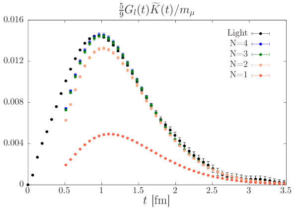
A challenge one eventually faces in exploiting lattice spectroscopy information is that the number of states required to saturate the TMR correlator at a given $t_{c}$ increases with decreasing pion masses and (roughly proportionally) with the volume. However, for the ensembles used in this work, the number of states needed is at most four.

Finite-size effects on $a_{\mu}^{\rm hvp}$ in the time-momentum representation

We now come to the closely related issue of the finite-size effect on the observable $a_{\mu}^{\rm hvp}$ calculated in the time-momentum representation. At asymptotically large volumes, the finite-size effect is of order $e^{-m_{\pi}L}$ and can be computed in chiral perturbation theory Aubin and Blum (2007); Francis et al. (2013); Aubin et al. (2016). At low pion masses, the leading finite-size effect is expected to come from the $\pi\pi$ channel, and thus affects the isovector channel only, $G^{I=1}(t)$. Working in the flavour decomposition of Eq. (3), we take this observation into account by applying $10/9$ of the isovector finite-size correction to the connected light-quark contribution, and $-1/9$ of the same correction to the disconnected contribution.

Looking at the finite-size effect on the correlator as a function of Euclidean time, it has been pointed out Bernecker and Meyer (2011); Francis et al. (2013) that for a given spatial box size $L$, the tail of the correlator is affected by an unsuppressed finite-size effect. One may define a time $t_{i}$ beyond which the finite-size effect becomes sizeable. While $t_{i}$ grows with $L$, we find that the overall finite-size effect on $a_{\mu}^{\rm hvp}$ is dominated by the tail in our present calculation.

For $m_{\pi}L=4-5$, the tail of the finite-volume isovector correlator is accurately described by the contribution of a handful of energy eigenstates; this point will be illustrated in Fig. 2. On the other hand, the tail of the infinite-volume correlator can be obtained from the timelike pion factor. Thus, knowledge of this form factor allows one to correct the tail of the isovector correlator Bernecker and Meyer (2011). In this work, we apply the same finite-size correction method as in our previous calculation Della Morte et al. (2017), parameterizing the pion form factor with the Gounaris-Sakurai (GS) model Gounaris and Sakurai (1968). While too simplistic a model for a study of the form factor for its own sake Feng et al. (2015); Andersen et al. (2019), we expect it to be sufficient for the purpose of reducing the residual finite-size effects to a level that is small compared to our current statistical precision. We emphasize that we only use the GS parametrization of the pion form factor for the finite-size correction, and not for the treatment of the tail of the correlators.

The chiral dependence of $a_{\mu}^{\rm hvp}$

The TMR correlator for non-interacting pions was given in Ref. Francis et al. (2013). For massless pions, it is given by $G(t)={1}/(24\pi^{2}|t|^{3})$; combined with the asymptotic form of the QED kernel for a finite muon mass, $\widetilde{K}(t)\sim 2\pi^{2}t^{2}$, this contribution generates a logarithmic divergence, which is made finite by a small but finite pion mass and then yields

$$a_{\mu}^{\rm hvp}{\sim}\frac{\alpha^{2}}{24\pi^{2}}\log\frac{m_{\mu}^{2}}{4m_{\pi}^{2}},\qquad m_{\pi}\to 0,~{}m_{\mu}{\rm~{}fixed}.$$ (16)

This result and further terms in the expansion have been derived in Golterman et al. (2017), where the systematics of the chiral extrapolation has been studied in detail. The asymptotic form (16) only becomes a decent approximation for $m_{\pi}/m_{\mu}$ well below $1/10$. Thus this logarithmic divergence is largely irrelevant when describing the pion-mass dependence of $a_{\mu}^{\rm hvp}$ in the range $130<m_{\pi}/{\rm MeV}<300$. On the other hand, if $m_{\mu}\ll m_{\pi}$ and both are small compared to the $\rho$ meson mass, one finds the leading behaviour

$$a_{\mu}^{\rm hvp}{\sim}\frac{\alpha^{2}}{90\pi^{2}}\frac{m_{\mu}^{2}}{4m_{\pi}^{2}},\qquad m_{\mu}\ll m_{\pi}\ll m_{\rho}.$$ (17)

It turns out that this asymptotic form is rather robust, holding down to fairly small values of $m_{\pi}/m_{\mu}$. In fact, within the framework of chiral perturbation theory at next-to-leading order underlying Eqs. (16) and (17), the combination $(1+\frac{4m_{\pi}^{2}}{m_{\mu}^{2}})a_{\mu}^{\rm hvp}$ only varies by $2\%$ for $m_{\pi}/m_{\mu}$ in the interval $[1.25,3.0]$ relevant to our lattice calculations.

At physical quark masses, the overall magnitude of expression (17) is enhanced by the (squared) pion form factor at timelike kinematics. In addition, the contribution of the $\pi\pi$ states with a center-of-mass energy well below the $\rho$-meson mass is numerically subdominant compared to the resonant contribution. The $\rho$-meson mass depends only mildly on the light-quark mass, and thus the steep behaviour predicted by Eq. (17) as a function of $m_{\pi}$ is superimposed on a larger, more slowly varying contribution. In our chiral extrapolations, presented in section IV, we use these observations to construct suitable fit ansätze for the chiral extrapolation.

The singular chiral behaviour comes from the isovector channel, while we expect the isoscalar channel to have a much milder dependence on the pion mass. Working in the basis of Eq. (3), the singular chiral behaviour is split between the connected light-quark contribution and the disconnected contribution. Indeed, in the limit that $m_{\mu}$ and $m_{\pi}$ are much smaller than the hadronic scale, we have $a_{\mu}^{{\rm hvp,\,disc}}=-\frac{1}{9}a_{\mu}^{{\rm hvp}}$, and hence, from Eq. (17),

$$a_{\mu}^{{\rm hvp,\,disc}}{\sim}-\frac{\alpha^{2}}{810\pi^{2}}\frac{m_{\mu}^{2}}{4m_{\pi}^{2}},\qquad m_{\mu}\ll m_{\pi}\ll m_{\rho}.$$ (18)

For orientation, we note that if one inserts the physical pion mass into this expression, one obtains $a_{\mu}^{{\rm hvp,\,disc}}=-10\times 10^{-10}$, and we expect this value to be further enhanced by the pion form factor. The important point is that the singular chiral behaviour present in the connected light-quark contribution to $a_{\mu}^{\rm hvp}$ must be present in the disconnected contribution as well, with a relative factor of $-1/10$.

III Results

In this section we describe the main features of the TMR correlators obtained on the different lattice ensembles with a view to computing $a_{\mu}^{\rm hvp}$. Particular attention is devoted to the correlators at Euclidean times in the range [1.5, 4.0] fm. In the rescaling of the muon mass, we use the values of $af_{\pi}$ values given in Table 6, corrected for finite-size effects Colangelo et al. (2005) and interpolated via a global fit in the pion mass and the lattice spacing.

III.1 The quark-connected contributions

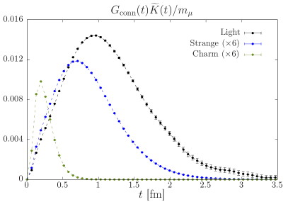
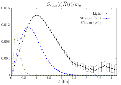
The integrand of Eq. (1) for the connected light, strange and charm contributions is displayed in Fig. 1 for our two ensembles with quark masses closest to their physical values. The left (right) panel corresponds to a pion mass of about 200 MeV (131 MeV). The light contribution is clearly very dominant; note that the charm and strange contributions have been scaled by a factor of six for better visibility. On a given ensemble, the integrand peaks at increasingly longer distances as one goes from the charm to the strange to the light quarks, and the tail becomes more extended. At the same time, the statistical precision deteriorates. Comparing the left to the right panel, it is clear that the light contribution becomes harder to determine with the desired precision as the physical quark masses are approached. Nevertheless, these plots by themselves do not fully reflect all the known constraints on the TMR correlator, which is well known to be given by a sum of decaying exponentials with positive coefficients, as discussed in section II.5.

Figure 1: Integrand of Eq. (1) in the time-momentum representation for the connected light, strange and charm contributions. Left: ensemble D200 with a pion mass of 200 MeV. Right: ensemble E250 at the physical pion mass. For better visibility, the strange and charm contributions have been scaled by a factor six. The displayed discretization is the local-local one for the light and strange contributions, and the local-conserved one for the charm. The muon mass is the $f_{\pi}$ rescaled one for the light integrand and the physical one for the strange and charm integrands.

Figure 2: Reconstruction of the TMR correlator at long distances using a dedicated spectroscopy analysis on ensemble D200. The same gauge configurations are used for the spectroscopy and for the TMR correlator calculation.

Having described the state-of-the-art methods to handle the tail of the correlation function in section II.5, we now describe how we applied these methods to our data. For the strange and charm quark contributions, the TMR correlator is determined so accurately that practically no particular treatment of the tail is needed. We apply the bounding method, Eq. 14 with $N=0$, and obtain the results given in Table 4.

As for the connected contribution of the light quarks, our choice for the final analysis is again the bounding method on all ensembles; the only exception is the physical-pion-mass ensemble E250, to which we return below. In applying Eq. (14), we employ the expression containing the effective mass as a lower bound, and use as an estimate for the lowest-lying energy level in the channel the energy obtained by a one-exponential fit to the tail of the TMR correlator. On ensemble D200, on which the ground state lies clearly below the $\rho$ mass and has a relatively weak coupling to the vector current, we use the auxiliary spectroscopy calculation to determine its energy. We find it to be close to, but slightly below the value corresponding to two non-interacting pions, $E_{0}^{\rm free}\equiv 2[\left({2\pi}/{L}\right)^{2}+m_{\pi}^{2}]^{1/2}$. Table 6 contains our results for the connected contributions of the light quarks.

As discussed in detail in the next subsection, the improved statistical precision gained by exploiting spectroscopic information can be quite significant for light pion masses, $m_{\pi}\lesssim 200\,$MeV. Indeed we find that on the physical mass ensemble E250, on which we do not have direct spectroscopic information, we cannot achieve a comparable control over the statistical and systematic error with the simplest variant of the bounding method. Therefore we proceed as follows. The isovector vector energy levels computed on ensembles N203, N200 and D200 allow us to determine the scattering phase in the $I=\ell=1$ $\pi\pi$ channel Andersen et al. (2019) for energies up to the four-pion threshold via the Lüscher formalism Lüscher (1991). The scattering phase is well described by the effective range formula,

$$\frac{k^{3}}{E}\cot\delta_{11}=\frac{4k_{\rho}^{5}}{m_{\rho}^{2}\Gamma_{\rho}}\Big{(}1-\frac{k^{2}}{k_{\rho}^{2}}\Big{)},$$ (19)

with $k\equiv\frac{1}{2}\sqrt{E^{2}-4m_{\pi}^{2}}$ and $k_{\rho}$ being the value of $k$ for $E=m_{\rho}$. The parameters $m_{\rho}$ and $\Gamma_{\rho}$ correspond to the $\rho$ meson mass and width. Furthermore, it has been observed in lattice simulations that parameterizing the width by

$$\Gamma_{\rho}=\frac{g_{\rho\pi\pi}^{2}}{6\pi}\,\frac{k_{\rho}^{3}}{m_{\rho}^{2}},$$ (20)

the coupling $g_{\rho\pi\pi}$ only has a weak pion-mass dependence. Therefore, we extrapolate the parameters $(m_{\rho},g_{\rho\pi\pi})$ determined on the ensembles N203, N200 and D200 (see Table 8) to obtain their values for the pion mass corresponding to ensemble E250. Using these values, we can predict the low-lying energy levels $E_{n}$ on ensemble E250 by using the Lüscher correspondence between them and the scattering phase in reverse. In order to obtain an extension of the TMR correlator on E250, we then fit the squared amplitudes $Z_{n}^{2}$, given the energy levels. Note that this can be formulated as a linear fit.

In our final choice of parameters, we fit the TMR correlator on E250 in the interval $26<t/a<37$. Then the TMR is summed from $t=0$ to $t=28a$ and the multi-exponential extension is used beyond that time. The numbers given for E250 in Table 6 are the results from this procedure.

Figure 3: Bounding method with the contribution of $N=0$ (method (1), left) and $N=2$ (method (2), right) states subtracted on ensemble D200 for the local-local correlator and the $f_{\pi}$-rescaled muon mass. Results based on 1100 gauge configurations.

III.2 Comparing different methods of extracting $a_{\mu}^{{\rm hvp},l}$ on ensemble D200

Figure 4: Determination of $a_{\mu}^{{\rm hvp},l}$ with the $f_{\pi}$-rescaled muon mass using the extension of the connected light (local-local) correlator using $N=2$ energy levels on ensemble D200. On the left (method 3), the amplitudes corresponding to energy levels were predetermined in a spectroscopy calculation, while on the right (method 4), they are fitted to the TMR correlator. Results based on 1100 gauge configurations.

On ensemble D200 at $m_{\pi}=200\,$MeV, we have detailed information on the scattering phase and the timelike pion form factor. We can thus test the validity of the procedure we applied on the physical pion-mass ensemble E250, described in the previous subsection.

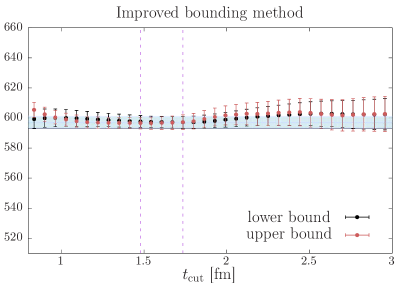
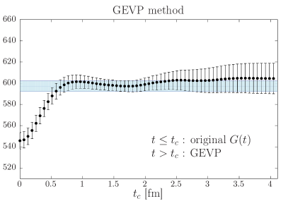
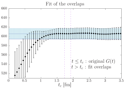
Thus on D200 we apply and compare four different methods to handle the tail of the light connected correlator:

1. the bounding method without subtractions ($N=0$);

2. the bounding method after subtracting the contribution of $N=2$ states;

3. the extension of the correlator using the auxiliary information on the first two energy levels $E_{n}$ and their amplitudes $Z_{n}$;

4. the extension of the correlator using the auxiliary information on the first two energy levels $E_{n}$, but fitting the amplitudes to the TMR correlator.

One motivation for comparing these particular methods is that on E250, we cannot apply the second or third method, while the first method would result in a large statistical error. Therefore, we apply the last method on E250, and presently test whether it gives consistent results on ensemble D200.

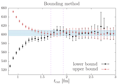
Fig. 3 compares the results for $a_{\mu}^{\rm hvp}$ from methods (1) and (2), as a function of the time $t_{c}$ at which the upper and lower bounds start to be used instead of the TMR correlator itself. The values are consistent with each other, however method (2) yields a significantly reduced statistical uncertainty. This outcome is not surprising, since important auxiliary information is used in method (2).

A comparison of methods (3) and (4) is shown in Fig. 4, showing the resulting $a_{\mu}^{\rm hvp}$ as a function of the time $t_{c}$ at which the TMR correlator is replaced by the multi-exponential extension. The result of method (4) is consistent with that of method (3), albeit with an enlarged statistical uncertainty. In addition we have checked that the values of the amplitudes of the first two states as extracted from the fit in method (4) are well consistent with their direct spectroscopic determination. Table 2 presents the results obtained on D200 with the four different methods.

Table 2: Dependence of the D200 result for $10^{10}\times a_{\mu}^{{\rm hvp},l}$ on the methods described in the text, using the local-local TMR correlator.

Method	No rescaling	With $f_{\pi}$ rescaling
1.	605.9(6.3)	604.2(7.4)
2.	599.0(4.0)	597.1(5.2)
3.	599.4(3.9)	597.7(5.0)
4.	607.7(11.8)	605.7(11.8)

III.3 Finite-volume effects

Figure 5: Testing the finite-size correcting procedure described in the main text on the ensembles N101 and H105 at a pion mass of 280 MeV. The scale-setting uncertainty is not displayed, since both ensembles have the same lattice spacing.

As explained in section II.5, in the isospin basis, we would correct the $I=1$ correlator for finite-size effects stemming from the $\pi\pi$ states, and neglect such effects on the $I=0$ correlator. However, we work in the basis of Eq. (3). In this basis, such a correction corresponds to applying an additive finite-size correction to the connected light contribution ($\frac{5}{9}G_{l}(t)$), weighted by a factor of $10/9$ relative to the correction of the $I=1$ correlator. At the same time, the disconnected contribution $G_{\rm disc}$ must be corrected by $-1/9$ of the $I=1$ correction. It is indeed well known that the tail of $G_{\rm disc}(t)$ is given by $(-1/9)G^{I=1}(t)$ Francis et al. (2013).

The $I=1$ finite-size corrections are given in Table 7 for every ensemble. They are computed as in Della Morte et al. (2017), assuming a GS parametrization of the pion form factor. However, in contrast to Della Morte et al. (2017), the parameters of the GS parametrization are obtained either by fitting the tail of the TMR correlator using the relations between the $(E_{n},Z_{n})$ and the pion form factor Lüscher (1991); Meyer (2011), or by using the results for $m_{\rho}$ and $g_{\rho\pi\pi}$ from a dedicated pion form factor calculation, when available. This concerns ensembles C101, N401, N203, N200, D200 and J303.

We have neglected finite-size effects for the connected strange contribution, except for the SU(3) symmetric ensembles, where finite-size effects are the same as for the light-connected contribution. Similarly, no finite-volume correction is applied to the charm-quark contribution.

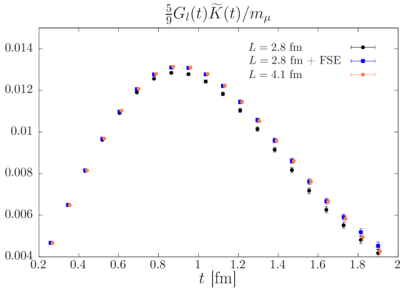
We have performed a direct lattice calculation of the FSE on two ensembles, N101 and H105, with different volumes, $L=2.8\,$fm and 4.1 fm, at a common pion mass of 280 MeV. Figure 5 shows that a finite-size effect is clearly visible and statistically significant. After the finite-size correction obtained via the GS model for the pion form factor, the two correlators are in excellent agreement. This test gives us confidence that the finite-size correction we apply is reliable at our level of statistical precision.

Figure 6: Integrand of Eq. (1) in the time-momentum representation for the disconnected contribution on ensemble N200, using the local-local discretization and the physical muon mass.

III.4 The quark-disconnected contribution

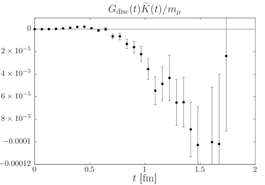
We have computed the quark-disconnected contribution on a number of lattice ensembles, namely H105, N401, N203, N200, D200, N302. A typical integrand is shown in Fig. 6. The signal for the quark disconnected contribution is lost around $t=1.5\,$fm. Given that the absolute error of the integrand for $a_{\mu}^{\rm hvp}$ grows asymptotically, it is clear that additional information constraining the tail of the disconnected TMR correlator is mandatory.

We have therefore adopted the following strategy. In our $N_{\rm f}=2+1$ simulations, the isoscalar correlator $G^{I=0,c\!\!/}(t)$ of the $(u,d,s)$ quarks admits a positive spectral representation analogous to Eq. (13), with positive prefactors multiplying the exponentials. We expect that on the ensembles on which we have computed the disconnected diagrams, the dominant exponential in a large window of Euclidean times corresponds to the $\omega$ meson mass. As we did not perform a dedicated calculation of the $\omega$ mass, we use our determination of the $\rho$ resonance mass. Since the latter is slightly lower than the $\omega$ mass, this is a conservative choice. We can therefore apply the bounding method in the following form,

$$0\leq G^{I=0,c\!\!/}(t)\leq G^{I=0,c\!\!/}(t_{c})e^{-m_{\rho}(t-t_{c})},\qquad t\geq t_{c}.$$ (21)

In order to quote a value $a_{\mu}^{\rm hvp,disc}$ for the quark-disconnected contribution to $a_{\mu}^{\rm hvp}$, we subtract the connected light and strange contributions from the isoscalar contribution $a_{\mu}^{{\rm hvp},I=0,c\!\!/}$,

$$a_{\mu}^{\rm hvp,disc}=a_{\mu}^{{\rm hvp},I=0,c\!\!/}-\frac{1}{10}a_{\mu}^{{\rm hvp},l}-a_{\mu}^{{\rm hvp},s}.$$ (22)

Our results for $a_{\mu}^{\rm hvp,disc}$ are listed in Table 5 in Appendix A.

IV Results at the physical point

Having determined the various contributions to $a_{\mu}^{\rm hvp}$ on a number of gauge ensembles, we proceed to extrapolate these results to the continuum and to the physical pion mass, $m_{\pi}=134.97\,$MeV. We use as chiral expansion variable the dimensionless ratio

$$\widetilde{y}=\frac{m_{\pi}^{2}}{16\pi^{2}f_{\pi}^{2}},$$ (23)

where $m_{\pi}$ and $f_{\pi}$ have been determined on each ensemble.

IV.1 The connected strange and charm contributions

Figure 7: Extrapolation of the connected strange and charm contributions to $a_{\mu}^{\rm hvp}$ with a muon mass fixed to its physical value. The black curve represents the chiral dependence in the continuum, and the black point the final result at the physical pion mass.

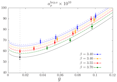
For the strange-quark contribution, the statistical error (excluding the lattice spacing uncertainty) is below 1% for all the ensembles, and in many cases below 0.5%, typically for those ensembles with close-to-physical quark masses. See Table 4. The error is therefore dominated by the scale-setting uncertainty, which enters through the combination $tm_{\mu}$ in the integrand (1). We extrapolate the results of the individual ensembles to the physical point using the fit ansatz

$$a_{\mu}^{{\rm hvp},s}(a,\widetilde{y},d)=a_{\mu}^{{\rm hvp},s}(0,\widetilde{y}_{\rm exp})+\delta_{d}\;a^{2}+\gamma_{1}(\widetilde{y}-\widetilde{y}_{\rm exp})+\gamma_{2}\,(\widetilde{y}\log{\widetilde{y}}-\widetilde{y}_{\rm exp}\log\widetilde{y}_{\rm exp}).$$ (24)

The index $d$ labels the discretization, local-local or local-conserved. We observe a rather mild continuum extrapolation and both discretizations are in very good agreement. The fit goes perfectly through our physical mass ensemble and our final result for the connected strange-quark contribution is

$$a_{\mu}^{{\rm hvp},s}=(54.5\pm 2.4\pm 0.6)\times 10^{-10},$$ (25)

where the first error is statistical and the second is the systematic error from the chiral extrapolation. The latter is estimated from the difference between the results obtained if one includes or excludes ensembles with $m_{\pi}>300\,$MeV. The chiral and continuum extrapolation is illustrated in the left panel of Fig. 7.

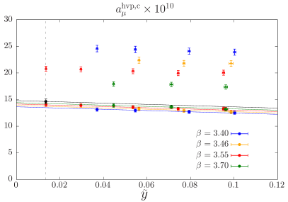
For the charm-quark contribution, the statistical error is below 0.3% for all the ensembles, and the error on the tuning of the charm hopping parameter is of similar magnitude. The error is again dominated by the scale-setting uncertainty. As can be seen on the right panel of Fig. 7, the lattice discretization of the correlator using two local vector currents leads to large cut-off effects: we observe a discretization effect of almost 70% at our coarsest lattice spacing. By contrast, for the local-conserved discretization the discretization effect is only 8%. Thus we prefer not to use the local-local discretization in our continuum extrapolation of the connected charm contribution. Furthermore, the data also suggest a very flat chiral behaviour, and we therefore use the fit ansatz

$$a_{\mu}^{{\rm hvp},c}(a,\widetilde{y})=a_{\mu}^{{\rm hvp},c}(0,\widetilde{y}_{\rm exp})+\delta\;a^{2}+\gamma_{1}(\widetilde{y}-\widetilde{y}_{\rm exp}).$$ (26)

At the physical point, we obtain

$$a_{\mu}^{{\rm hvp},c}=(14.66\pm 0.45\pm 0.06)\times 10^{-10},$$ (27)

where the first error is statistical and the second is the systematic error induced by the chiral extrapolation. The chiral and continuum extrapolation is illustrated in Fig. 7 (right panel).

A comparison of the strange and charm contributions to $a_{\mu}^{\rm hvp}$ with recent publications is shown in Fig. 10.

IV.2 The connected light-quark contribution

Figure 8: Extrapolation of the connected light contribution to $a_{\mu}^{\rm hvp}$, using the physical value of the muon mass in the kernel $\widetilde{K}(t)$ on all ensembles (left panel), and using the rescaled mass $m_{\mu}^{\rm phys}\cdot\frac{f_{\pi}^{\rm latt}}{f_{\pi}^{\rm phys}}$ (right panel). The result of the fit based on Eq. (28c) is shown. The black curve represents the chiral dependence in the continuum, and the black point the final result at the physical pion mass.

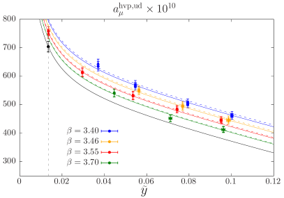
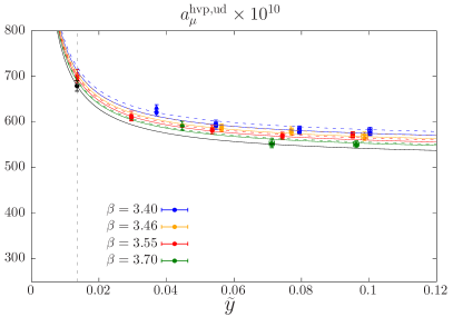
We have achieved a statistical error of just over two percent on $a_{\mu}^{{\rm hvp},l}$ on the physical-mass ensemble E250, and of $1.0-1.2\%$ on all other ensembles. An important role of the other ensembles is to constrain the continuum limit, which would be very costly to achieve directly at the physical pion mass. Our lattice data points are displayed as a function of $\widetilde{y}$ in Fig. 8, with and without the rescaling of the muon mass with $f_{\pi}$. We observe that the rescaled data on the right panel has a reduced dependence on $\widetilde{y}$, as well as on the lattice spacing. We therefore decide to use the rescaled data for our primary analysis, but also perform the analysis of the unrescaled data in parallel for comparison.

The expected chiral behaviour of the light connected contribution is reviewed in section II.5. Taking into account these considerations, we have used the following ansätze to simultaneously extrapolate our results to the continuum and to physical quark masses:

$$a_{\mu}^{{\rm hvp},l}(a,\widetilde{y},d) =a_{\mu}^{{\rm hvp},l}(0,\widetilde{y}_{\exp})+\delta_{d}\,a^{2}+\gamma_{1}\,\left(\widetilde{y}-\widetilde{y}_{\exp}\right)+\gamma_{2}\,\left(\log\widetilde{y}-\log\widetilde{y}_{\exp}\right),$$ (28a)

$$a_{\mu}^{{\rm hvp},l}(a,\widetilde{y},d) =a_{\mu}^{{\rm hvp},l}(0,\widetilde{y}_{\exp})+\delta_{d}\,a^{2}+\gamma_{3}\,\left(\widetilde{y}-\widetilde{y}_{\exp}\right)+\gamma_{4}\,\left(\widetilde{y}^{2}-\widetilde{y}_{\exp}^{2}\right),$$ (28b)

$$a_{\mu}^{{\rm hvp},l}(a,\widetilde{y},d) =a_{\mu}^{{\rm hvp},l}(0,\widetilde{y}_{\exp})+\delta_{d}\,a^{2}+\gamma_{5}\,\left(\widetilde{y}-\widetilde{y}_{\exp}\right)+\gamma_{6}\,\left(1/\widetilde{y}-1/\widetilde{y}_{\exp}\right),$$ (28c)

$$a_{\mu}^{{\rm hvp},l}(a,\widetilde{y},d) =a_{\mu}^{{\rm hvp},l}(0,\widetilde{y}_{\exp})+\delta_{d}\,a^{2}+\gamma_{7}\,\left(\widetilde{y}-\widetilde{y}_{\exp}\right)+\gamma_{8}\,\left(\widetilde{y}\log\widetilde{y}-\widetilde{y}_{\exp}\log\widetilde{y}_{\exp}\right),$$ (28d)

where $d$ is a label for the local-local or local-conserved correlator. All ansätze contain four parameters to be fitted, including an O($a^{2}$) term to account for discretization errors. Ansatz (b) assumes a purely polynomial behaviour in the variable $\widetilde{y}$, while fit (d) allows for a non-analytic $\widetilde{y}\log\widetilde{y}$ term. The latter ansatz was used in our previous $N_{\rm f}=2$ calculation Della Morte et al. (2017). Ansätze (a) and (c) are directly motivated by the discussion in section II.5, (a) containing the logarithmic singularity that appears in the limit $m_{\pi}\to 0$ at fixed muon mass, while (c) contains the $1/m_{\pi}^{2}$ term relevant in the regime $m_{\mu}\ll m_{\pi}\ll m_{\rho}$.

We give the results we obtain from these four ansätze, with and without rescaling $m_{\mu}$, in Table 3. We have performed these fits either including all ensembles, or imposing cuts on $\widetilde{y}$, corresponding to pion masses below 360 MeV or, alternatively, below 300 MeV. Focusing first on the rescaled data, we note that fits (a), (c) and (d) yield $\chi^{2}/{\rm d.o.f.}\approx 1.0$ while fit (b) produces higher values of around 1.6. With the pion-mass cut at 360 MeV, one sees that results (a) and (c) show good consistency and yield somewhat larger values of $a_{\mu}^{{\rm hvp},l}$ than fits (b) and (d). Given the more singular chiral behaviour of ansätze (a) and (c), this outcome is not unexpected. Looking at the stability of the final value for $a_{\mu}^{{\rm hvp},l}$ as a function of the pion-mass cut, we observe excellent stability in the case of fits (a) and (c), while the results of fits (b) and (d) systematically drift upward as a stronger pion-mass cut is imposed. With the strongest cut, $m_{\pi}<300\,$MeV, all four ansätze yield the same result within half a standard deviation. In view of the greater stability of fits (a) and (c) against pion-mass cuts, and the stronger theoretical motivation underlying them, we choose to average the results of fit (a) and (c) with the cut $m_{\pi}<360\,$MeV for our final central value. As a systematic error, we take the full difference between the results of these fits, and thus our final result for the connected light-quark contribution is

$$a_{\mu}^{{\rm hvp},l}=(674\pm 12\pm 5)\times 10^{-10}.$$ (29)

A few further remarks are in order. It is important to note that the results of fits (a) and (c) are in very good agreement with the values of $a_{\mu}^{{\rm hvp},l}$ directly obtained on ensemble E250 with the rescaled muon mass; see Table 6. We also remark that the statistical uncertainty on the final result Eq. (29) is only 20% lower than the statistical uncertainties on E250; we conclude that the chiral extrapolation of our results obtained at heavier pion masses, which tend to be more precise, does not lead to an artificially small final uncertainty. A comparison with the extrapolated results obtained from the standard kernel, shown in the left part of Table 3, shows that the latter lie systematically higher than the rescaled ones. Their statistical uncertainty is larger by about 50% than in the unrescaled case. Still, when combining statistical and systematic uncertainties in quadrature of Eq. (29), the central value of fit (c) only lies 1.6 standard deviations higher than our final central value Eq. (29).

Table 3: Results of the connected light-quark contribution in units of $10^{-10}$ using different fits and cuts. Left: using the standard kernel. Right: using the rescaling of the muon mass using $f_{\pi}$.

	Standard kernel			Kernel with rescaling using $f_{\pi}$
	cut 300 MeV	cut 360 MeV	no cut	cut 300 MeV	cut 360 MeV	no cut
Fit Eq. (28a)	700(22)	695(19)	700(18)	675(14)	671(11)	671(10)
Fit Eq. (28b)	700(23)	689(19)	683(17)	669(14)	656(09)	645(07)
Fit Eq. (28c)	700(22)	697(19)	704(18)	677(14)	676(12)	681(11)
Fit Eq. (28d)	700(22)	692(19)	692(17)	672(14)	663(10)	657(08)

IV.3 The quark-disconnected contribution

Figure 9: Extrapolation of the disconnected contribution to $a_{\mu}^{\rm hvp}$ in the SU(3)-breaking variable $\Delta_{2}\equiv m_{K}^{2}-m_{\pi}^{2}$. The data points for the local-local and the local-conserved discretizations are shown. A linear fit (straight black line), as well as a fit based on ansatz (30) are shown.

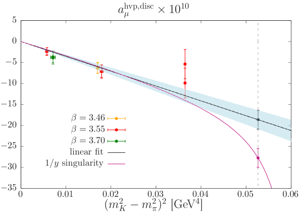
The quark-disconnected contributions have been computed on a subset of the gauge ensembles, as described in Section II.2. Three ensembles at the same lattice spacing – N203, N200 and D200 – allow us to study the chiral behaviour. Two other ensembles, N401 and N302, enable us to constrain the discretization effects.

The quark-disconnected contribution vanishes exactly for the ensembles generated at the SU(3) symmetric point. In fact, it is a double zero in the SU(3) breaking combination $(m_{s}-m_{l})$. Since our ensembles follow a chiral trajectory at fixed bare average quark mass $(2m_{{\rm q},l}+m_{{\rm q},s})$, we can consider the values of $a_{\mu}^{\rm disc}$ as being to a good approximation a function of the single variable $m_{K}^{2}-m_{\pi}^{2}$. The results of all five ensembles are thus displayed in Fig. 9 as a function of $\Delta_{2}^{\,2}$, where $\Delta_{2}\equiv m_{K}^{2}-m_{\pi}^{2}$, since close to the SU(3) symmetric point, the dependence of $a_{\mu}^{\rm disc}$ on $\Delta_{2}^{\,2}$ is linear. We observe that discretization effects are negligible at the current level of precision. The result of an extrapolation to the physical point $\Delta_{2}=0.227\,\mathrm{GeV}^{2}$ assuming a linear proportionality to $\Delta_{2}^{\,2}$ is $a_{\mu}^{{\rm hvp,\,disc}}=-18.6(2.2)\times 10^{-10}$.

As discussed below Eq. (18), the disconnected contribution has a singular behaviour in the limit $m_{\pi}\to 0$, closely related to the corresponding behaviour of the connected light contribution. Therefore, we consider the possibility that the disconnected contribution contains a term with precisely the dependence given in Eq. (18). In order to make this term consistent with the double zero of the disconnected correlator at $\Delta_{2}=0$, we fix $\hat{M}^{2}\equiv\frac{1}{2}m_{\pi}^{2}+m_{K}^{2}$ to its physical value, express $m_{\pi}^{2}$ through the variable $\Delta_{2}$ and use the ansatz

$$a_{\mu}^{{\rm hvp,\,disc}}(\Delta_{2})=\gamma_{8}\Delta_{2}^{\,2}-\frac{\alpha^{2}m_{\mu}^{2}}{3240\pi^{2}}\cdot\frac{3}{2}\Big{[}\frac{1}{\hat{M}^{2}-\Delta_{2}}-\frac{\Delta_{2}}{\hat{M}^{4}}-\frac{1}{\hat{M}^{2}}\Big{]}.$$ (30)

Fitting the single free parameter $\gamma_{8}$, we obtain $a_{\mu}^{{\rm hvp,\,disc}}=-27.7(2.2)\times 10^{-10}$. From Fig. 18, it is clear that both the linear fit in $\Delta_{2}^{\,2}$ and the one based on ansatz (30) are consistent with the lattice data. While a singular chiral behaviour must be present in $a_{\mu}^{{\rm hvp,\,disc}}$, the ansatz (30) may lead to an overestimate of this effect. Therefore, we quote as our final result the average of the linear and the chirally singular fit,

$$a_{\mu}^{{\rm hvp,\,disc}}=(-23.2\pm 2.2\pm 4.5)\times 10^{-10},$$ (31)

where the first error is statistical and the second is a systematic error associated with the extrapolation to the physical point, taken to be the half-distance between the two extrapolated values.

IV.4 The total $a_{\mu}^{\rm hvp}$

In summary, adding up the connected light, strange and charm contributions as well as the quark-disconnected contribution, our result for $a_{\mu}^{\rm hvp}$ in isospin-symmetric QCD at $m_{\pi}=134.97\,$MeV and $f_{\pi}=92.4\,\mathrm{MeV}$ is

$$a_{\mu}^{\rm hvp}=(720.0\pm 12.4\pm 6.8)\times 10^{-10},$$ (32)

where the first error is statistical and the second is the systematic error. The latter is dominated by the chiral extrapolation of the light-connected and the disconnected contributions. The result Eq. (32) does not contain any correction for QED or strong isospin-breaking effects. For now, we do not attempt to include such a correction, but rather add (in quadrature) a systematic uncertainty of $7.2\times 10^{-10}$ corresponding to a recent lattice calculation of these effects Giusti et al. (2019). This then leads to our final result given in Eq. (33) below.

V Discussion and comparison

Figure 10: Compilation of lattice results for the connected contributions to $a_{\mu}^{\rm hvp}$ from individual charm, strange and light quarks (left to right). In the rightmost panel, the full results, including (where available) the contributions from quark-disconnected diagrams and corrections due to isospin-breaking, are compared to the phenomenological determination of Ref. Keshavarzi et al. (2018), represented by the red vertical band. Our result is compared to the calculations labelled FNAL-HPQCD-MILC 19 Chakraborty et al. (2014, 2018); Davies et al. (2019), PACS 19 Shintani and Kuramashi (2019), ETMC 19 Giusti et al. (2017, 2018, 2019), RBC/UKQCD 18 Blum et al. (2018), BMW 17 Borsanyi et al. (2018), as well as our previous calculation in two-flavour QCD Della Morte et al. (2017) (Mainz/CLS 17).

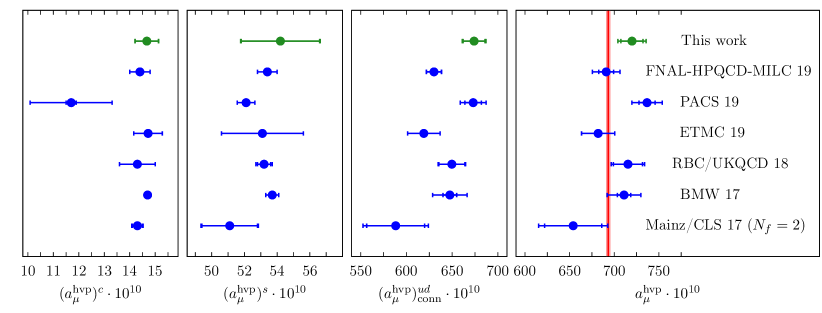
In this paper we have presented a calculation of the hadronic vacuum polarization contribution to $a_{\mu}$ based on gauge ensembles with $N_{f}=2+1$ flavours of O($a$) improved Wilson quarks. Our final result is

$$a_{\mu}^{\rm hvp}=(720.0\pm 12.4_{\rm stat}\,\pm 9.9_{\rm syst})\cdot 10^{-10},$$ (33)

where the first error is statistical, and the second is an estimate of the total systematic uncertainty, which also accounts for the fact that the corrections due to isospin breaking have not been included. We thus find that the overall error of our determination is 2.2%. In Fig. 10 we compare our results to those of several other recent lattice calculations Della Morte et al. (2017); Borsanyi et al. (2018); Blum et al. (2018); Giusti et al. (2019); Shintani and Kuramashi (2019); Davies et al. (2019). While our estimate is at the higher end of lattice results, we note that the direct difference with the result based on dispersion theory of Ref. Keshavarzi et al. (2018) is $26.6\pm 16.0$, which amounts to $\sim 1.7$ standard deviations and may signal a slight tension.

There are several ways in which our result can be improved without relying on the obvious strategy of adding more ensembles and increasing the overall statistics. First, we have seen in section III.2 that the use of detailed spectroscopy information in the isovector channel is a huge advantage, as it nearly halves the statistical uncertainty in the estimate for $a_{\mu}^{{\rm hvp},l}$ on ensemble D200. This is the result of either constructing the vector correlator from the energies and overlaps determined via the GEVP or of using this information in the improved bounding method. Extending these calculations to more ensembles – in particular those with physical and near-physical pion masses – will boost the statistical accuracy and reliability significantly.

Second, we have pointed out that it is advantageous to split the correlator into isovector and isoscalar components according to Eq. (4) rather than focussing on separating the contributions from individual quark flavours. One reason is that the singular chiral behaviour expected from Eq. (17) is shared between the light quark connected and the disconnected contributions. This will help to better constrain the pion mass dependence of the quark-disconnected contribution, which is often still obtained from an extrapolation to the physical point from a set of results at heavier pion masses. The decomposition according to isospin also gives a better handle on finite-volume effects, which are partly compensated between the light connected and disconnected contributions. This is of particular importance, since finite-volume corrections for the disconnected part of the vector correlator could be sizeable but, to our knowledge, have not been estimated so far.

The third refinement concerns the determination of isospin-breaking corrections. We stress again that our final estimate in Eq. (33) is valid at a well-defined reference point of the isospin-symmetric theory, given by the mass of the neutral pion in the continuum limit. The determination of the corrections due to isospin breaking relies on the definition of an alternative reference point that is consistent with the effects induced by a non-vanishing mass splitting among the up and down quarks and the coupling between quarks and photons. This requires an adjustment of bare parameters and the re-evaluation of a number of observables that enter the calculation of $a_{\mu}^{\rm hvp}$. An account of the status of our activities in this direction is given in Refs. Risch and Wittig (2018a, b). In the absence of a complete evaluation, we have refrained from simply adding results for the isospin-breaking correction from the literature. Instead, we have opted for an additional systematic error which is as large as the correction determined in Giusti et al. (2019).

As the community awaits the first results from the E989 experiment at Fermilab, it is remarkable that several collaborations using different setups and discretizations of the QCD action obtain largely consistent estimates for $a_{\mu}^{\rm hvp}$ with overall errors at the level of 2%. However, the collection of available results does not allow for a firm conclusion as to whether the phenomenological estimate or the so-called “No New Physics” scenario is confirmed.

Appendix A Results for the individual contributions to $a_{\mu}^{\rm hvp}$ and auxiliary calculations

Table 4: Values of the connected strange and charm contribution to $a_{\mu}^{\rm hvp}$, in units of $10^{-10}$, for the local-local (${\scriptstyle\rm LL}$) and for the local-conserved (${\scriptstyle\rm CL}$) discretizations of the correlation function. For the strange, the symmetric lattice derivative is used for the improvement term, while the ‘away’ derivative is used for the charm (see section II.3). In addition, the charm hopping parameter is given, as well as the mass-dependent renormalization factor $Z_{\rm V}^{(c)}$ for the charm vector current. The bounding method is used to handle the tail of the correlator, as described in section III.1. For the charm contribution, the first error is statistical, the second comes from the tuning of the charm hopping parameter. The scale-setting uncertainty is not included at this stage.

id	$a_{\mu}^{({\scriptscriptstyle\rm LL}),s}$	$a_{\mu}^{({\scriptscriptstyle\rm CL}),s}$	$a_{\mu}^{({\scriptscriptstyle\rm LL}),c}$	$a_{\mu}^{({\scriptscriptstyle\rm CL}),c}$	$\kappa_{\rm c}$	$Z_{\rm V}^{(c)}$
H101	91.09(42)	92.47(41)	23.909(31)(56)	12.541(21)(31)	0.122897(18)	1.20324(11)(25)
H102	81.10(37)	82.47(36)	24.088(20)(81)	12.709(20)(46)	0.123041(26)	1.19743(08)(20)
U101∗	71.08(44)	72.40(44)	24.510(28)(61)	13.051(19)(35)	0.123244(19)	1.18964(08)(15)
H105∗	71.94(31)	73.27(31)	24.437(42)(61)	12.996(29)(35)	0.123244(19)	1.18964(08)(15)
N101	72.14(23)	73.50(23)	24.414(57)(61)	12.996(38)(35)	0.123244(19)	1.18964(08)(15)
C101	68.37(18)	69.70(18)	24.580(43)(39)	13.140(29)(22)	0.123361(12)	1.18500(05)(10)
B450	87.27(49)	88.41(48)	21.793(24)(70)	12.668(18)(43)	0.125095(22)	1.12972(06)(16)
S400	77.72(34)	78.78(34)	21.808(27)(64)	12.919(20)(41)	0.125252(20)	1.11159(13)(18)
N401	70.80(20)	71.81(20)	22.390(39)(50)	13.248(29)(32)	0.125439(15)	1.11412(04)(19)
H200∗	83.02(87)	83.69(86)	20.018(37)(56)	13.248(28)(40)	0.127579(16)	1.04843(03)(19)
N202	88.83(71)	89.61(69)	20.052(39)(56)	13.280(30)(40)	0.127579(16)	1.04843(03)(53)
N203	76.17(37)	76.91(36)	19.969(30)(39)	13.252(22)(28)	0.127714(11)	1.04534(03)(19)
N200	67.90(23)	68.60(22)	20.323(42)(26)	13.577(32)(18)	0.127858(07)	1.04012(03)(13)
D200	62.20(15)	62.93(15)	20.677(39)(22)	13.895(30)(16)	0.127986(06)	1.03587(04)(11)
E250	59.64(14)	60.36(14)	20.798(02)(21)	14.027(02)(15)	0.128052(05)	1.03310(01)(10)
N300	81.03(69)	81.44(68)	17.367(34)(73)	13.159(29)(58)	0.130099(18)	0.97722(03)(12)
N302	70.11(31)	70.53(30)	17.839(28)(38)	13.606(23)(30)	0.130247(09)	0.97241(03)(10)
J303	62.87(21)	63.27(20)	17.931(49)(31)	13.870(40)(27)	0.130362(09)	0.96037(10)(19)

Table 5: Results for $a_{\mu}^{\rm hvp,disc}$, with and without rescaling the muon mass.

	No rescaling		With rescaling
id	$a_{\mu}^{({\scriptscriptstyle\rm LL}),l}$	$a_{\mu}^{({\scriptscriptstyle\rm CL}),l}$	$a_{\mu}^{({\scriptscriptstyle\rm LL}),l}$	$a_{\mu}^{({\scriptscriptstyle\rm CL}),l}$
N401	-5.41(1.25)	-5.50(1.21)	-5.76(1.30)	-5.85(1.26)
N203	-1.60(0.77)	-1.65(0.80)	-1.85(0.88)	-1.91(0.92)
N200	-5.50(1.32)	-5.55(1.46)	-5.99(1.46)	-6.05(1.61)
D200	-3.79(3.51)	-8.32(3.57)	-3.78(3.50)	-8.30(3.56)
N302	-1.55(1.16)	-1.77(1.23)	-1.84(1.39)	-2.10(1.47)

Table 6: Values of the connected light contribution to $a_{\mu}^{\rm hvp}$, in units of $10^{-10}$, for the local-local (${\scriptstyle\rm LL}$) and for the local-conserved (${\scriptstyle\rm CL}$) discretizations of the correlation function, as described in the main text. The symmetric lattice derivative of the improvement term is used. In addition, the pion mass and the pion decay constant are given, some of them taken from Ref. Gérardin et al. (2019b). No FSE correction has been applied on any data in the table. The treatment of the long-distance part of the correlator is described in section III.1. In the “No rescaling” columns, the scale-setting error has not been included. In the “With rescaling” columns, the statistical fluctuations of the $f_{\pi}$ determination are taken into account.

			No rescaling		With rescaling
id	$am_{\pi}$	$a\sqrt{2}f_{\pi}$	$a_{\mu}^{({\scriptscriptstyle\rm LL}),l}$	$a_{\mu}^{({\scriptscriptstyle\rm CL}),l}$	$a_{\mu}^{({\scriptscriptstyle\rm LL}),l}$	$a_{\mu}^{({\scriptscriptstyle\rm CL}),l}$
H101	0.1818(07)	0.06458(29)	455.5(2.0)	462.4(2.0)	571.9(4.4)	580.5(4.5)
H102	0.1547(08)	0.06151(27)	495.0(3.5)	501.9(3.4)	572.2(4.7)	580.2(4.7)
H105∗	0.1224(11)	0.05802(39)	548.7(5.9)	555.4(6.0)	576.4(8.0)	583.4(8.1)
N101	0.1217(06)	0.05832(30)	562.8(4.3)	568.9(4.2)	589.8(6.8)	596.4(6.7)
C101	0.0967(08)	0.05535(37)	625.0(6.7)	633.3(7.5)	612.9(6.9)	621.9(7.3)
B450	0.1608(05)	0.05750(27)	436.3(2.4)	442.0(2.4)	556.8(4.7)	564.3(4.8)
S400	0.1357(05)	0.05463(21)	481.4(3.8)	486.4(3.8)	564.3(5.2)	570.2(5.2)
N401	0.1104(06)	0.05324(17)	543.8(4.2)	548.9(4.1)	581.5(5.3)	587.0(5.2)
H200∗	0.1362(07)	0.04805(27)	413.6(4.5)	417.8(4.3)	532.0(5.5)	537.5(5.3)
N202	0.1335(05)	0.04884(18)	441.8(3.0)	445.9(2.9)	567.9(4.4)	573.2(4.3)
N203	0.1126(04)	0.04699(16)	479.1(3.3)	483.2(3.3)	564.6(5.0)	569.4(5.1)
N200	0.0920(05)	0.04454(18)	520.0(5.3)	524.4(5.0)	571.8(6.1)	576.6(5.8)
D200	0.0649(04)	0.04254(18)	600.3(5.0)	604.3(5.9)	598.6(6.3)	602.4(6.3)
E250	0.0422(04)	0.04089(19)	735.1(14.6)	726.3(14.8)	679.7(14.8)	671.6(14.9)
N300	0.1063(04)	0.03811(13)	404.1(3.4)	406.0(3.3)	540.6(5.5)	543.2(5.4)
N302	0.0872(04)	0.03570(19)	436.6(4.4)	438.8(4.4)	535.4(6.5)	538.1(6.5)
J303	0.0651(03)	0.03412(14)	526.6(7.4)	527.4(7.2)	577.5(8.5)	578.3(8.4)

Table 7: Estimates of the finite-size effects $\Delta a_{\mu}^{\rm hvp}\equiv a_{\mu}^{\rm hvp}(L=\infty)-a_{\mu}^{\rm hvp}(L)=\Delta a_{\mu}^{<}(t_{i})+\Delta a_{\mu}^{>}(t_{i})$ on the isovector contribution $a_{\mu}^{{\rm hvp},I=1}$ in the TMR in units of $10^{-10}$. We used the value $t_{i}=(m_{\pi}L/4)^{2}/m_{\pi}$, as in Della Morte et al. (2017), to which we refer for unexplained notation. The parameters of the GS model are obtained by fitting the tail of the correlation function using the Lüscher formalism. When there are two lines, the second line corresponds to the GS parameters extracted from a direct lattice calculation of the timelike pion form factor Andersen et al. (2019). The FSE effects are given both with and without rescaling of the muon mass via $f_{\pi}$.

		GS parameters		No rescaling		With rescaling
id	$t_{i}~{}$[fm]	$m_{\rho}/m_{\pi}$	$g_{\rho\pi\pi}$	$\Delta a_{\mu}^{<}(t_{i})$	$\Delta a_{\mu}^{>}(t_{i})$	$\Delta a_{\mu}^{<}(t_{i})$	$\Delta a_{\mu}^{>}(t_{i})$
H101	1.04	2.101(103)	4.60(42)	0.29	2.0(0.4)	0.37	2.4(0.5)
H102	0.86	2.307(07)	4.88(02)	0.40	5.6(0.1)	0.47	6.3(0.1)
U101∗	0.35	2.698(290)	5.23(52)	0.11	49.0(10.8)	0.12	51.4(11.3)
H105∗	0.69	2.743(110)	5.01(24)	0.46	16.6(1.4)	0.48	17.3(1.5)
N101	1.55	2.792(10)	4.93(04)	0.61	1.8(0.1)	0.64	1.9(0.1)
C101	1.21	3.362(73)	4.92(12)	0.92	8.1(0.3)	0.90	8.0(0.3)
	1.21	3.395(26)	5.67(17)	0.92	7.9(0.2)	0.90	7.8(0.2)
B450	0.76	2.100(10)	4.86(04)	0.27	4.4(0.1)	0.35	5.6(0.1)
S400	0.69	2.299(41)	5.01(14)	0.38	11.0(0.5)	0.45	12.8(0.6)
N401	1.22	2.716(25)	5.08(06)	0.60	3.7(0.1)	0.65	3.9(0.1)
	1.22	2.717(16)	5.84(17)	0.60	3.6(0.1)	0.65	3.8(0.1)
H200∗	0.58	2.095(02)	4.86(07)	0.27	10.5(0.2)	0.40	13.3(0.2)
N202	1.22	2.016(04)	5.21(07)	0.23	1.1(0.1)	0.30	1.4(0.2)
N203	1.03	2.398(13)	4.91(05)	0.40	3.2(0.1)	0.47	3.7(0.1)
	1.03	2.382(11)	6.03(13)	0.40	3.1(0.1)	0.47	3.6(0.1)
N200	0.84	2.833(20)	4.98(05)	0.50	9.2(0.2)	0.60	9.3(0.8)
	0.85	2.733(16)	5.94(10)	0.49	9.6(0.2)	0.55	10.6(0.2)
D200	1.09	3.737(72)	5.26(10)	1.00	13.4(0.4)	0.99	13.3(0.4)
	1.09	3.877(34)	6.16(19)	1.00	12.8(0.2)	0.99	12.7(0.2)
E250	1.54	5.270(42)	5.59(03)	1.88	20.7(0.2)	1.74	19.4(0.2)
	1.54	5.955(84)	6.06(21)	1.88	19.1(0.2)	1.74	17.9(0.2)
N300	0.75	2.100(01)	4.89(08)	0.27	4.6(0.2)	0.36	6.1(0.3)
N302	0.65	2.301(07)	5.59(08)	0.36	13.0(0.3)	0.45	15.8(0.3)
J303	0.85	2.993(02)	5.17(03)	0.61	12.4(0.1)	0.67	13.4(0.1)
	0.85	3.090(24)	6.33(16)	0.61	11.4(0.5)	0.67	12.4(0.5)

Table 8: Results of spectroscopy calculations in the isovector vector channel for the parameters $m_{\rho}$ and $g_{\rho\pi\pi}$ of the $\rho$ meson. See Eqs. (19) and (20). For ensemble J303, the data from Andersen et al. (2019) has been rebinned and analyzed using the jackknife method.

	$am_{\rho}$	$m_{\rho}/m_{\pi}$	$g_{\rho\pi\pi}$	source
C101	0.3327(23)	3.395(26)	5.67(17)	Andersen et al. (2019)
N401	0.2989(16)	2.717(16)	5.84(17)	Andersen et al. (2019)
N203	0.2682(13)	2.382(11)	6.03(13)	New data
N200	0.2522(13)	2.733(16)	5.94(10)	Andersen et al. (2019)
D200	0.2501(12)	3.839(18)	6.065(92)	New data
J303	0.2020(15)	3.090(24)	6.33(16)	Andersen et al. (2019)

Appendix B Determination of the charm-quark hopping parameter

We list in Table 9 the values of the $c\bar{s}$ pseudoscalar meson masses determined for different values of the charm hopping parameter. The ‘physical’ value of the charm-quark hopping parameter is determined by the condition that the $c\bar{s}$ meson mass match the physical value of the $D_{s}$ meson mass, $m_{D_{s}}=1972\,$MeV.

id		Interpolation	Simulations
H101	$\kappa$	0.122897(18)	0.12320	0.12290	0.12260	0.12230
	$am_{D_{s}}$	0.8615	0.8513(6)	0.8614(6)	0.8714(6)	0.8813(6)
H102	$\kappa$	0.123041(26)	0.12330	0.12300	0.12270	0.12240
	$am_{D_{s}}$	0.8615	0.8528(9)	0.8629(9)	0.8729(9)	0.8828(9)
N101	$\kappa$	0.123244(19)	0.12360	0.12340	0.12320	0.12300
	$am_{D_{s}}$	0.8615	0.8495(6)	0.8563(6)	0.8630(6)	0.8697(6)
C101	$\kappa$	0.123361(12)	0.12400	0.12370	0.12340	0.12310
	$am_{D_{s}}$	0.8615	0.8467(4)	0.8534(4)	0.8602(4)	0..8669(4)
B450	$\kappa$	0.125095(22)	0.12530	0.12510	0.12490	0.12470
	$am_{D_{s}}$	0.7615	0.7543(8)	0.7614(8)	0.7683(8)	0.7752(8)
S400	$\kappa$	0.125252(20)	0.12570	0.12550	0.12530	0.12510
	$am_{D_{s}}$	0.7615	0.7457(7)	0.7528(7)	0.7599(7)	0.7669(7)
N401	$\kappa$	0.125439(15)	0.12570	0.12550	0.12530	0.12510
	$am_{D_{s}}$	0.7615	0.7523(5)	0.7594(5)	0.7564(5)	0.7734(5)
N202	$\kappa$	0.127579(16)	0.12775	0.12765	0.12755	0.12745
	$am_{D_{s}}$	0.6410	0.6347(6)	0.6384(6)	0.6421(6)	0.6458(6)
N203	$\kappa$	0.127714(11)	0.12790	0.12770	0.12750	0.12730
	$am_{D_{s}}$	0.6410	0.6341(4)	0.6416(4)	0.6490(4)	0.6563(4)
N200	$\kappa$	0.127858(07)	0.12810	0.12790	0.12770	0.12750
	$am_{D_{s}}$	0.6410	0.6320(3)	0.6395(3)	0.6469(3)	0.6543(3)
D200	$\kappa$	0.127986(06)	0.12820	0.12810	0.12800	0.12790
	$am_{D_{s}}$	0.6410	0.6330(2)	0.6367(2)	0.6405(2)	0.6442(2)
E250	$\kappa$	0.128052(05)	0.12830	0.12810	0.12790	0.12770
	$am_{D_{s}}$	0.6410	0.6317(2)	0.6392(2)	0.6467(2)	0.6541(2)
N300	$\kappa$	0.130099(18)	0.12970	0.13000	0.13030	0.13060
	$am_{D_{s}}$	0.4969	0.5126(7)	0.5008(7)	0.4888(7)	0.4766(7)
N302	$\kappa$	0.130247(09)	0.13000	0.13030	0.13060	0.13090
	$am_{D_{s}}$	0.4969	0.5066(3)	0.4947(3)	0.4827(3)	0.4704(3)
J303	$\kappa$	0.130362(09)	0.13020	0.13040	0.13060	0.13080
	$am_{D_{s}}$	0.4969	0.5033(4)	0.4954(4)	0.4873(4)	0.4792(3)

Table 9: Values of the $c\bar{s}$ pseudoscalar meson masses determined for different values of the charm hopping parameter, and its interpolation to the physical $D_{s}$ meson mass.

References

- Bennett et al. (2006) G. W. Bennett et al. (Muon g-2), Phys. Rev. D73, 072003 (2006), eprint hep-ex/0602035.
- Jegerlehner and Nyffeler (2009) F. Jegerlehner and A. Nyffeler, Phys.Rept. 477, 1 (2009), eprint 0902.3360.
- Blum et al. (2013) T. Blum, A. Denig, I. Logashenko, E. de Rafael, B. Lee Roberts, et al. (2013), eprint 1311.2198.
- Jegerlehner (2017) F. Jegerlehner, The Anomalous Magnetic Moment of the Muon (Springer Tracts Mod. Phys., vol. 274, 2017).
- Grange et al. (2015) J. Grange et al. (Muon g-2) (2015), eprint 1501.06858.
- Mibe (2011) T. Mibe (J-PARC g-2), Nucl. Phys. Proc. Suppl. 218, 242 (2011).
- Meyer and Wittig (2019) H. B. Meyer and H. Wittig, Prog. Part. Nucl. Phys. 104, 46 (2019), eprint 1807.09370.
- Blum et al. (2017) T. Blum, N. Christ, M. Hayakawa, T. Izubuchi, L. Jin, C. Jung, and C. Lehner, Phys. Rev. Lett. 118, 022005 (2017), eprint 1610.04603.
- Asmussen et al. (2018) N. Asmussen, A. Gérardin, A. Nyffeler, and H. B. Meyer, in 15th International Workshop on Tau Lepton Physics (TAU2018) Amsterdam, Netherlands, September 24-28, 2018 (2018), eprint 1811.08320.
- Colangelo et al. (2018) G. Colangelo, M. Hoferichter, M. Procura, and P. Stoffer, EPJ Web Conf. 175, 01025 (2018), eprint 1711.00281.
- Bruno et al. (2015) M. Bruno et al., JHEP 02, 043 (2015), eprint 1411.3982.
- Bali et al. (2016a) G. S. Bali, E. E. Scholz, J. Simeth, and W. Söldner (RQCD), Phys. Rev. D94, 074501 (2016a), eprint 1606.09039.
- Mohler et al. (2018) D. Mohler, S. Schaefer, and J. Simeth, EPJ Web Conf. 175, 02010 (2018), eprint 1712.04884.
- Risch and Wittig (2018a) A. Risch and H. Wittig, EPJ Web Conf. 175, 14019 (2018a), eprint 1710.06801.
- Risch and Wittig (2018b) A. Risch and H. Wittig, in 36th International Symposium on Lattice Field Theory (Lattice 2018) East Lansing, MI, United States, July 22-28, 2018 (2018b), eprint 1811.00895.
- Blum (2003) T. Blum, Phys.Rev.Lett. 91, 052001 (2003), eprint hep-lat/0212018.
- Bernecker and Meyer (2011) D. Bernecker and H. B. Meyer, Eur.Phys.J. A47, 148 (2011), eprint 1107.4388.
- Lüscher (1991) M. Lüscher, Nucl. Phys. B364, 237 (1991).
- Meyer (2011) H. B. Meyer, Phys.Rev.Lett. 107, 072002 (2011), eprint 1105.1892.
- Della Morte et al. (2017) M. Della Morte, A. Francis, V. Gülpers, G. Herdoíza, G. von Hippel, H. Horch, B. Jäger, H. B. Meyer, A. Nyffeler, and H. Wittig, JHEP 10, 020 (2017), eprint 1705.01775.
- Della Morte et al. (2018) M. Della Morte et al., EPJ Web Conf. 175, 06031 (2018), eprint 1710.10072.
- Feng et al. (2011) X. Feng, K. Jansen, M. Petschlies, and D. B. Renner, Phys.Rev.Lett. 107, 081802 (2011), eprint 1103.4818.
- Lüscher and Schaefer (2013) M. Lüscher and S. Schaefer, Comput.Phys.Commun. 184, 519 (2013), eprint 1206.2809.
- Bulava and Schaefer (2013) J. Bulava and S. Schaefer, Nucl.Phys. B874, 188 (2013), eprint 1304.7093.
- Bruno et al. (2017) M. Bruno, T. Korzec, and S. Schaefer, Phys. Rev. D95, 074504 (2017), eprint 1608.08900.
- Lüscher and Schaefer (2011) M. Lüscher and S. Schaefer, JHEP 07, 036 (2011), eprint 1105.4749.
- Wilcox (2000) W. Wilcox, in Numerical Challenges in Lattice Quantum Chromodynamics, edited by A. Frommer, T. Lippert, B. Medeke, and K. Schilling (Springer Berlin Heidelberg, 2000), vol. 15 of Lecture Notes in Computational Science and Engineering, pp. 127–141, ISBN 978-3-540-67732-1, eprint hep-lat/9911013.
- Foley et al. (2005) J. Foley, K. Jimmy Juge, A. O’Cais, M. Peardon, S. M. Ryan, et al., Comput.Phys.Commun. 172, 145 (2005), eprint hep-lat/0505023.
- Andersen et al. (2019) C. Andersen, J. Bulava, B. Hörz, and C. Morningstar, Nucl. Phys. B939, 145 (2019), eprint 1808.05007.
- Stathopoulos et al. (2013) A. Stathopoulos, J. Laeuchli, and K. Orginos (2013), eprint 1302.4018.
- Djukanovic et al. (2019) D. Djukanovic, K. Ottnad, J. Wilhelm, and H. Wittig (2019), eprint 1903.12566.
- Lüscher et al. (1996) M. Lüscher, S. Sint, R. Sommer, and P. Weisz, Nucl. Phys. B478, 365 (1996), eprint hep-lat/9605038.
- Bhattacharya et al. (2006) T. Bhattacharya, R. Gupta, W. Lee, S. R. Sharpe, and J. M. S. Wu, Phys. Rev. D73, 034504 (2006), eprint hep-lat/0511014.
- Gérardin et al. (2019a) A. Gérardin, T. Harris, and H. B. Meyer, Phys. Rev. D99, 014519 (2019a), eprint 1811.08209.
- Dalla Brida et al. (2019) M. Dalla Brida, T. Korzec, S. Sint, and P. Vilaseca, Eur. Phys. J. C79, 23 (2019), eprint 1808.09236.
- Harris and Meyer (2015) T. Harris and H. B. Meyer, Phys. Rev. D92, 114503 (2015), eprint 1506.05248.
- Lehner (2016) C. Lehner, RBRC Workshop on Lattice Gauge Theories (2016).
- Borsanyi et al. (2018) S. Borsanyi et al. (Budapest-Marseille-Wuppertal), Phys. Rev. Lett. 121, 022002 (2018), eprint 1711.04980.
- Blum et al. (2018) T. Blum, P. A. Boyle, V. Gülpers, T. Izubuchi, L. Jin, C. Jung, A. Jüttner, C. Lehner, A. Portelli, and J. T. Tsang (RBC, UKQCD), Phys. Rev. Lett. 121, 022003 (2018), eprint 1801.07224.
- Aubin and Blum (2007) C. Aubin and T. Blum, Phys.Rev. D75, 114502 (2007), eprint hep-lat/0608011.
- Francis et al. (2013) A. Francis, B. Jäger, H. B. Meyer, and H. Wittig, Phys.Rev. D88, 054502 (2013), eprint 1306.2532.
- Aubin et al. (2016) C. Aubin, T. Blum, P. Chau, M. Golterman, S. Peris, and C. Tu, Phys. Rev. D93, 054508 (2016), eprint 1512.07555.
- Gounaris and Sakurai (1968) G. Gounaris and J. Sakurai, Phys.Rev.Lett. 21, 244 (1968).
- Feng et al. (2015) X. Feng, S. Aoki, S. Hashimoto, and T. Kaneko, Phys. Rev. D91, 054504 (2015), eprint 1412.6319.
- Golterman et al. (2017) M. Golterman, K. Maltman, and S. Peris, Phys. Rev. D95, 074509 (2017), eprint 1701.08685.
- Golowich and Kambor (1995) E. Golowich and J. Kambor, Nucl. Phys. B447, 373 (1995), eprint hep-ph/9501318.
- Amoros et al. (2000) G. Amoros, J. Bijnens, and P. Talavera, Nucl. Phys. B568, 319 (2000), eprint hep-ph/9907264.
- Colangelo et al. (2005) G. Colangelo, S. Durr, and C. Haefeli, Nucl.Phys. B721, 136 (2005), eprint hep-lat/0503014.
- Alexandrou et al. (2017) C. Alexandrou, L. Leskovec, S. Meinel, J. Negele, S. Paul, M. Petschlies, A. Pochinsky, G. Rendon, and S. Syritsyn, Phys. Rev. D96, 034525 (2017), eprint 1704.05439.
- Fu and Wang (2016) Z. Fu and L. Wang, Phys. Rev. D94, 034505 (2016), eprint 1608.07478.
- Guo et al. (2016) D. Guo, A. Alexandru, R. Molina, and M. Döring, Phys. Rev. D94, 034501 (2016), eprint 1605.03993.
- Wilson et al. (2015) D. J. Wilson, R. A. Briceno, J. J. Dudek, R. G. Edwards, and C. E. Thomas, Phys. Rev. D92, 094502 (2015), eprint 1507.02599.
- Bali et al. (2016b) G. S. Bali, S. Collins, A. Cox, G. Donald, M. Göckeler, C. B. Lang, and A. Schäfer (RQCD), Phys. Rev. D93, 054509 (2016b), eprint 1512.08678.
- Giusti et al. (2019) D. Giusti, V. Lubicz, G. Martinelli, F. Sanfilippo, and S. Simula (2019), eprint 1901.10462.
- Keshavarzi et al. (2018) A. Keshavarzi, D. Nomura, and T. Teubner, Phys. Rev. D97, 114025 (2018), eprint 1802.02995.
- Chakraborty et al. (2014) B. Chakraborty, C. T. H. Davies, G. C. Donald, R. J. Dowdall, J. Koponen, G. P. Lepage, and T. Teubner (HPQCD), Phys. Rev. D89, 114501 (2014), eprint 1403.1778.
- Chakraborty et al. (2018) B. Chakraborty et al. (Fermilab Lattice, LATTICE-HPQCD, MILC), Phys. Rev. Lett. 120, 152001 (2018), eprint 1710.11212.
- Davies et al. (2019) C. T. H. Davies et al. (Fermilab Lattice, LATTICE-HPQCD, MILC) (2019), eprint 1902.04223.
- Shintani and Kuramashi (2019) E. Shintani and Y. Kuramashi (2019), eprint 1902.00885.
- Giusti et al. (2017) D. Giusti, V. Lubicz, G. Martinelli, F. Sanfilippo, and S. Simula, JHEP 10, 157 (2017), eprint 1707.03019.
- Giusti et al. (2018) D. Giusti, F. Sanfilippo, and S. Simula, Phys. Rev. D98, 114504 (2018), eprint 1808.00887.
- Boyle et al. (2017) P. Boyle, M. Chuvelev, G. Cossu, C. Kelly, C. Lehner, and L. Meadows (2017), eprint 1711.04883.
- Edwards and Joo (2005) R. G. Edwards and B. Joo (SciDAC, LHPC, UKQCD), Nucl. Phys. Proc. Suppl. 140, 832 (2005), eprint hep-lat/0409003.
- Gérardin et al. (2019b) A. Gérardin, H. B. Meyer, and A. Nyffeler (2019b), eprint 1903.09471.