Translational control of gene expression via interacting feedback loops. Supplemental Material.

1 Protein Dynamics and Effective Vacancy of the Start Site

Protein complex formation and loss, respectively, can be represented as follows:

$$\underbrace{\text{P}+\text{P}+\ldots\text{P}}_{n}\autorightleftharpoons{r_{1}}{r_{2}}n\text{P},\quad\text{P}\autorightarrow{r}{}\emptyset$$

where P is protein, $n\geq 1$ proteins form a protein complex $n\text{P}$ and $r_{1},\,r_{2}$ and $r$ are rate constants, where $r_{1}$ has dimensions of $(\text{volume})^{n-1}/\text{time}$, and $r_{2}$ and $r$ have dimensions of 1/time. Applying a quasi-steady-state approximation for the complex concentration:

$$\dfrac{d[n\text{P}]}{dt}=r_{1}\left([\text{P}]\right)^{n}-r_{2}[n\text{P}]\approx 0\quad\Longrightarrow\quad[n\text{P}]=\dfrac{r_{1}}{r_{2}}\left([\text{P}]\right)^{n}=\dfrac{r_{1}}{r_{2}}\left(\dfrac{N}{V}\right)^{n},$$ (S1)

where $[\,\cdot\,]$ represents concentration, $N$ denotes the number of molecules of P, and $V$ denotes the cell volume. The protein complex is assumed to bind and unbind from some location at the start site (SS) at rates $k_{1},k_{2}$, respectively:

$$n\text{P}+\text{SS}\autorightleftharpoons{k_{1}}{k_{2}}n\text{P}\cdot\text{SS}.$$ (S2)

Writing (S2) as a differential equation and applying the quasi-steady state approximation as above yields

$$\cfrac{d[n\text{P}\cdot\text{SS}]}{dt} =k_{1}[n\text{P}][\text{SS}]-k_{2}[n\text{P}\cdot\text{SS}]\approx 0$$

$$i.e. \quad[n\text{P}\cdot\text{SS}]=\frac{k_{1}}{k_{2}}[n\text{P}][\text{SS}].$$ (S3)

This quasi-steady state approximation leads to an effective vacancy of the SS from the perspective of ribosome binding events. The probability that the SS is vacant is equivalent to

$$\frac{[\text{SS}]}{[\text{SS}]+[n\text{P}\cdot\text{SS}]}=\frac{[\text{SS}]}{[\text{SS}]+\frac{k_{1}}{k_{2}}[n\text{P}][\text{SS}]}=\frac{k_{2}}{k_{2}+k_{1}[n\text{P}]},$$ (S4)

where we have used (S3). This probability can be written in terms the number of proteins, $N$, as follows. Using (S1) and (S4) it follows that the probability that the SS is free is

$$f(N):=\dfrac{1}{1+\left(N/\theta\right)^{n}},$$ (S5)

where $\theta=V\sqrt[n]{r_{2}k_{2}/r_{1}k_{1}}$.

2 Phases and Phase Boundaries

Maximal Current Phase: $\alpha_{eff},\,\beta_{eff}\geqslant 1/2$

$$\rho_{1}=1-\dfrac{1}{4\alpha_{eff}},\qquad\rho_{L}=\dfrac{1}{4\beta_{eff}},\qquad\rho=\frac{1}{2},\qquad J=\dfrac{1}{4}.$$ (S6)

Low Density Phase: $\alpha_{eff}<\beta_{eff},\,\alpha_{eff}<1/2$

$$\rho_{1}=\alpha_{eff},\qquad\rho_{L}=\dfrac{\alpha_{eff}(1-\alpha_{eff})}{\beta_{eff}},\qquad\rho=\alpha_{eff},\qquad J=\alpha_{eff}(1-\alpha_{eff}).$$ (S7)

High Density Phase: $\alpha_{eff}>\beta_{eff},\,\alpha_{eff}>1/2$

$$\rho_{1}=1-\dfrac{\beta_{eff}(1-\beta_{eff})}{\alpha_{eff}},\qquad\rho_{L}=1-\beta_{eff},\qquad\rho=1-\beta_{eff},\qquad J=\beta_{eff}(1-\beta_{eff}).$$ (S8)

In each case the corresponding steady state protein level is given by $N^{*}:=J/r$. We now define the phase boundaries in a series of lemmas. Proofs are lengthy and hence grouped in the next section for easier exposition.

Lemma 1

The Maximal Current Phase is defined by

$$\dfrac{\alpha}{2\alpha+k\left(1+I^{n}\right)}\leqslant\left\{\begin{aligned} &\beta&\leqslant\dfrac{\alpha k}{1+I^{n}-2\alpha}\quad&\text{if}\quad\alpha<\dfrac{1}{2}\left(1+I^{n}\right),\\ &\beta&\quad&\text{otherwise},\end{aligned}\right.$$ (S9)

where $I:=\frac{1}{4r\theta}$. Within this region,

$$\alpha_{eff}=\dfrac{\alpha}{1+I^{n}}+\dfrac{k}{2\left(\beta+\sqrt{\beta\left(\beta+\dfrac{k}{\alpha}\left(1+I^{n}\right)\right)}\right)}\quad\mbox{and}\quad\beta_{eff}=\dfrac{1}{2}\left(\beta+\sqrt{\beta\left(\beta+\dfrac{k}{\alpha}\left(1+I^{n}\right)\right)}\right).$$ (S10)

Remark 1

Note that the stacking of the left and right inequalities (S9) in case $\alpha<\dfrac{1}{2}\left(1+I^{n}\right)$ is necessary and therefore generates a lower bound for $\alpha$ and $\beta$ marked by the intersection of the two functions of $\alpha$. It is straightforward to compute this intersection:

$$(\alpha,\beta)=\left(\frac{1-k}{2}\left(1+I^{n}\right),\frac{1-k}{2}\right).$$ (S11)

Lemma 2

The Low Density Phase is defined by

$$\alpha<\left\{\begin{aligned} &\beta\left(1+\left(\dfrac{4I(\beta+k)(1-\beta)}{(1+k)^{2}}\right)^{n}\right)&\qquad&\text{if}\quad 2\beta+k<1,\\ &\dfrac{\beta}{2\beta+k}\left(1+I^{n}\right)&\qquad&\text{otherwise}.\end{aligned}\right.$$ (S12)

Within this region, there exists a unique, positive expression for $\alpha_{eff}$ that yields unique, positive expressions for $\beta_{eff}$ and $N^{*}$.

Lemma 3

The High Density Phase is defined by

$$\alpha>\left\{\begin{aligned} &\beta\left(1+\left(\dfrac{4I(\beta+k)(1-\beta)}{(1+k)^{2}}\right)^{n}\right)&\qquad&\text{if}\quad 2\beta+k<1,\\ &\dfrac{k\beta}{1-2\beta}\left(1+I^{n}\right)&\qquad&\text{otherwise},\end{aligned}\qquad\beta<\dfrac{1}{2}.\right.$$ (S13)

Within this region, there exist either one or three positive solutions, $\beta_{eff}$, that yield positive expressions for $\alpha_{eff}$ and $N^{*}$.

3 Proofs

Proof of Lemma 1 Substituting the effective rates into (S6) yields:

$$\beta_{eff} =\beta+k(1-\rho_{1})=\beta+k\left(1-\left(1-\dfrac{1}{4\alpha_{eff}}\right)\right)=\beta+\dfrac{k}{4}\dfrac{1}{\alpha_{eff}}.$$

Therefore, we obtain a quadratic equation for $\beta_{eff}$:

$$4^{n+1}\alpha(\theta r)^{n}\beta_{eff}^{2}-4^{n+1}\alpha\beta(\theta r)^{n}\beta_{eff}-k\beta\left((4\theta r)^{n}+1\right)=0.$$

Subsequently,

$$\beta_{eff}= \dfrac{1}{2}\left(\beta\pm\sqrt{\beta^{2}+\dfrac{k\beta\left((4\theta r)^{n}+1\right)}{4^{n}\alpha(\theta r)^{n}}}\right).$$

Since we require $\beta_{eff}$ to be positive and $\sqrt{\beta^{2}+\dfrac{k\beta\left((4\theta r)^{n}+1\right)}{4^{n}\alpha(\theta r)^{n}}}>\beta$, it follows that:

$$\beta_{eff}=\dfrac{1}{2}\left(\beta+\sqrt{\beta\left(\beta+\dfrac{k}{\alpha}\left(1+\left(\dfrac{1}{4\theta r}\right)^{n}\right)\right)}\right).$$ (S14)

Then $\alpha_{eff}$ is easy to obtain:

$$\alpha_{eff} =\dfrac{\alpha}{1+\left(\dfrac{1}{4\theta r}\right)^{n}}+\dfrac{k}{2\left(\beta+\sqrt{\beta\left(\beta+\dfrac{k}{\alpha}\left(1+\left(\dfrac{1}{4\theta r}\right)^{n}\right)\right)}\right)}.$$ (S15)

The maximal current phase is determined by the conditions $\alpha_{eff},\,\beta_{eff}\geqslant\dfrac{1}{2}$ i.e.:

$$\beta_{eff}=\dfrac{\beta+\sqrt{\beta\left(\beta+\dfrac{k}{\alpha}\left(1+\left(\dfrac{1}{4\theta r}\right)^{n}\right)\right)}}{2}\geqslant\dfrac{1}{2},$$

so $\sqrt{\beta\left(\beta+\dfrac{k}{\alpha}\left(1+\left(\dfrac{1}{4\theta r}\right)^{n}\right)\right)}\geqslant 1-\beta$. Since $1-\beta>0$ for $\beta<1$, we have

$$\beta\geqslant\dfrac{\alpha}{2\alpha+k\left(1+\left(\dfrac{1}{4\theta r}\right)^{n}\right)},$$ (S16)

and

$$\alpha_{eff}=\dfrac{\alpha}{1+\left(\dfrac{1}{4\theta r}\right)^{n}}+\dfrac{k}{2\left(\beta+\sqrt{\beta\left(\beta+\dfrac{k}{\alpha}\left(1+\left(\dfrac{1}{4\theta r}\right)^{n}\right)\right)}\right)}\geqslant\dfrac{1}{2},$$

namely,

$$\dfrac{k}{2\left(\beta+\sqrt{\beta\left(\beta+\dfrac{k}{\alpha}\left(1+\left(\dfrac{1}{4\theta r}\right)^{n}\right)\right)}\right)}\geqslant\dfrac{1}{2}-\dfrac{\alpha}{1+\left(\dfrac{1}{4\theta r}\right)^{n}}.$$ (S17)

If $\dfrac{1}{2}-\dfrac{\alpha}{1+\left(\dfrac{1}{4\theta r}\right)^{n}}\leqslant 0$, i.e., $\alpha\geqslant\dfrac{1}{2}\left(1+\left(\dfrac{1}{4\theta r}\right)^{n}\right)$, then (S17) is always true.

If $\alpha<\dfrac{1}{2}\left(1+\left(\dfrac{1}{4\theta r}\right)^{n}\right)$, we have:

$$k\geqslant 2\left(\dfrac{1}{2}-\dfrac{\alpha}{1+\left(\dfrac{1}{4\theta r}\right)^{n}}\right)\left(\beta+\sqrt{\beta\left(\beta+\dfrac{k}{\alpha}\left(1+\left(\dfrac{1}{4\theta r}\right)^{n}\right)\right)}\right),$$

subsequently,

$$k-\left(1-\dfrac{2\alpha}{1+\left(\dfrac{1}{4\theta r}\right)^{n}}\right)\beta\geqslant\left(1-\dfrac{2\alpha}{1+\left(\dfrac{1}{4\theta r}\right)^{n}}\right)\sqrt{\beta\left(\beta+\dfrac{k}{\alpha}\left(1+\left(\dfrac{1}{4\theta r}\right)^{n}\right)\right)}>0.$$ (S18)

From (S18), we have a weak condition

$$\beta\leqslant\dfrac{\alpha k}{1+\left(\dfrac{1}{4\theta r}\right)^{n}-2\alpha}.$$ (S19)

The result follows by grouping the inequalities determined above and on writing the final expression in terms of the intensity factor.

$\Box$

Proof of Lemma 2 Substituting the effective rates into (S7) yields:

$$\alpha_{eff}=\dfrac{\alpha}{1+\left(\dfrac{\alpha_{eff}(1-\alpha_{eff})}{\theta r}\right)^{n}}+k\dfrac{\alpha_{eff}(1-\alpha_{eff})}{\beta+k(1-\alpha_{eff})}.$$

Again after some manipulation we obtain:

$$P(\alpha_{eff}):=\beta\alpha_{eff}^{n+1}(1-\alpha_{eff})^{n}+(\theta r)^{n}(\beta+\alpha k)\alpha_{eff}-\alpha(\theta r)^{n}(\beta+k)=0.$$ (S20)

If there exist positive solutions, $\alpha_{eff}$, to (S20), then from (S7), $\beta_{eff}=\beta+k\left(1-\alpha_{eff}\right)$ and $N^{*}=\alpha_{eff}(1-\alpha_{eff})/r$. Next we consider the conditions for the existence of $\alpha_{eff}$ and thus define the phase boundary for the LD phase. LD phase is by defined by $\alpha_{eff}<\beta_{eff},\,\alpha_{eff}<\dfrac{1}{2}$. From $\alpha_{eff}<\beta_{eff}$, we have:

$$\alpha_{eff}<\beta_{eff}=\beta+k(1-\alpha_{eff}),\quad\Longrightarrow\quad(1+k)\alpha_{eff}<\beta+k,$$

therefore

$$\alpha_{eff}<\dfrac{\beta+k}{1+k}.$$ (S21)

On the other hand, we require $\alpha_{eff}<\dfrac{1}{2}$. Therefore $\alpha_{eff}<\min\left(\dfrac{1}{2},\,\dfrac{\beta+k}{1+k}\right)$.

If $\dfrac{\beta+k}{1+k}\geqslant\dfrac{1}{2}$, i.e., $2\beta+2k\geqslant 1+k$, $2\beta+k\geqslant 1$, then $\alpha_{eff}<\dfrac{1}{2}$. The derivative of $P$ with respect to $\alpha_{eff}$ is

$$P^{\prime} =\beta\alpha_{eff}^{n}(1-\alpha_{eff})^{n-1}\left(1-\alpha_{eff}+n(1-2\alpha_{eff})\right)+(\theta r)^{n}(\beta+\alpha k).$$

Since both $1-\alpha_{eff}$ and $1-2\alpha_{eff}$ are positive in $\left(0,\,\dfrac{1}{2}\right)$, so $P^{\prime}>0$ in $\left(0,\,\dfrac{1}{2}\right)$. Moreover, $P(0)=-\alpha(\theta r)^{n}(\beta+k)<0$. Therefore, a real, positive solution of (S20) exists if and only if $f\left(\dfrac{1}{2}\right)>0$ (in this case, the solution is unique). Now,

$$P\left(\dfrac{1}{2}\right) =\dfrac{(\theta r)^{n}}{2}\left(\beta\left(1+\left(\dfrac{1}{4\theta r}\right)^{n}\right)-\alpha(2\beta+k)\right),$$

so $P\left(\dfrac{1}{2}\right)>0$ requires $\beta\left(1+\left(\dfrac{1}{4\theta r}\right)^{n}\right)-\alpha(2\beta+k)>0$, namely,

$$\alpha<\dfrac{\beta}{2\beta+k}\left(1+\left(\dfrac{1}{4\theta r}\right)^{n}\right).$$ (S22)

If $\dfrac{\beta+k}{1+k}<\dfrac{1}{2}$, i.e., $2\beta+k<1$, then $\alpha_{eff}<\dfrac{\beta+k}{1+k}$. Since $P$ is increasing in $\left(0,\,\dfrac{1}{2}\right)$ and $P(0)<0$, so a solution of (S20) exists if and only if $P\left(\dfrac{\beta+k}{1+k}\right)>0$ (and again the solution is unique).

$$P\left(\dfrac{\beta+k}{1+k}\right) =\dfrac{(\beta+k)(\theta r)^{n}}{1+k}\left(\beta\left(\dfrac{(\beta+k)(1-\beta)}{\theta r(1+k)^{2}}\right)^{n}+\beta-\alpha\right)>0,$$

provided

$$\alpha<\beta\left(1+\left(\dfrac{(\beta+k)(1-\beta)}{\theta r(1+k)^{2}}\right)^{n}\right).$$ (S23)

The proof is complete by writing the inequalities in terms of the Intensity Factor.

$\Box$

Proof of Lemma 3 Substituting the effective rates into (S8) yields:

$$\beta_{eff} =\beta+k\dfrac{\beta_{eff}(1-\beta_{eff})}{\dfrac{\alpha}{1+\left(\dfrac{N}{\theta}\right)^{n}}+k\rho_{L}}=\beta+\dfrac{k\beta_{eff}(1-\beta_{eff})}{\dfrac{\alpha}{1+\left(\dfrac{\beta_{eff}(1-\beta_{eff})}{\theta r}\right)^{n}}+k(1-\beta_{eff})}.$$

Further algebra yields the equation

$$Q(\beta_{eff}):=k\beta\beta_{eff}^{n}\left(1-\beta_{eff}\right)^{n+1}-(k\beta+\alpha)(\theta r)^{n}\beta_{eff}+\beta(\theta r)^{n}(\alpha+k)=0.$$ (S24)

With $\beta_{eff}$ a solution of (S24), then from (S8), $\rho=1-\beta_{eff}$, $J=\beta_{eff}(1-\beta_{eff})$ and $N^{*}=\beta_{eff}(1-\beta_{eff})/r$. Hence, the effective initiation rate is given by

$$\alpha_{eff}=\dfrac{\alpha}{1+\left(\dfrac{\beta_{eff}(1-\beta_{eff})}{\theta r}\right)^{n}}+k\left(1-\beta_{eff}\right).$$

One of the HD conditions is $\beta_{eff}<\dfrac{1}{2}$, i.e. $\dfrac{1}{2}>\beta_{eff}=\beta+k(1-\rho_{1})>\beta$, namely, $\beta<\dfrac{1}{2}$. Moreover, from the second condition for HD $\alpha_{eff}>\beta_{eff}$, we have

$$\beta_{eff}=\beta+k\dfrac{\beta_{eff}(1-\beta_{eff})}{\alpha_{eff}}<\beta+k(1-\beta_{eff})\quad\Longrightarrow\quad(1+k)\beta_{eff}<\beta+k.$$

Therefore, we require $\beta_{eff}<\min\left\{\dfrac{1}{2},\,\dfrac{\beta+k}{1+k}\right\}$.

If $\dfrac{\beta+k}{1+k}\geqslant\dfrac{1}{2}$, i.e., $2\beta+k\geqslant 1$ then we need to check the existence of solutions to (S24) in $\left(0,\,\dfrac{1}{2}\right)$. To this end, note that

$$Q^{\prime} =k\beta\beta_{eff}^{n-1}\left(1-\beta_{eff}\right)^{n}\left(n-(2n+1)\beta_{eff}\right)-(k\beta+\alpha)(\theta r)^{n},$$

$$Q^{\prime\prime} =nk\beta\beta_{eff}^{n-2}\left(1-\beta_{eff}\right)^{n-1}\left(2(2n+1)\beta_{eff}^{2}-4n\beta_{eff}+n-1\right).$$

Thus, $Q^{\prime\prime}>0$ in $\left(0,\,\beta_{eff}^{-}\right)$ and $Q^{\prime\prime}<0$ in $\left[\beta_{eff}^{-},\,\dfrac{1}{2}\right)$ with the maximum of $Q^{\prime}$ obtained at $\beta_{eff}^{-}$. Moreover,

$$Q^{\prime}\left(0\right) =-(k\beta+\alpha)(\theta r)^{n}<0\quad\mbox{and}\quad Q^{\prime}\left(\dfrac{1}{2}\right)=-k\beta\dfrac{1}{4^{n}}-(k\beta+\alpha)(\theta r)^{n}<0.$$

If $Q^{\prime}\left(\beta_{eff}^{-}\right)<0$, then $Q^{\prime}<0$ ($Q$ is decreasing) in $\left(0,\,\dfrac{1}{2}\right)$. Besides, $Q(0)=\beta(\theta r)^{n}(\alpha+k)>0$. Thus, the solution of (S24) $Q=0$ exists if and only if $Q\left(\dfrac{1}{2}\right)<0$, and the solution is unique.

If $Q^{\prime}\left(\beta_{eff}^{-}\right)>0$, then there are two solutions to $Q^{\prime}=0$. Let $\beta_{eff}^{1}$ and $\beta_{eff}^{2}$ denote the solutions and $0<\beta_{eff}^{1}<\beta_{eff}^{2}<\dfrac{1}{2}$. Thus, $Q^{\prime}<0$ ($Q$ is decreasing) in $\left(0,\,\beta_{eff}^{1}\right)\cup\left(\beta_{eff}^{2},\,\dfrac{1}{2}\right)$, $Q^{\prime}>0$ ($Q$ is increasing) in $\left(\beta_{eff}^{1},\,\beta_{eff}^{2}\right)$. Moreover, $Q(0)=\beta(\theta r)^{n}(\alpha+k)>0$, and $Q\left(\beta_{eff}^{1}\right)$ is the local minimum. We have following cases.

(I) If $Q\left(\beta_{eff}^{1}\right)<0$ and $Q\left(\beta_{eff}^{2}\right)<0$, then $Q<0$ in $\left(\beta_{eff}^{1},\,\dfrac{1}{2}\right)$, there exists a unique solution to (S24) in $\left(0,\,\beta_{eff}^{1}\right)$. In this case, $Q\left(\dfrac{1}{2}\right)<0$.

(III) If $Q\left(\beta_{eff}^{1}\right)<0$ and $Q\left(\beta_{eff}^{2}\right)>0$, then (S24) has three solutions if $Q\left(\dfrac{1}{2}\right)<0$ or two solutions if $Q\left(\dfrac{1}{2}\right)>0$. If $Q\left(\dfrac{1}{2}\right)>0$, we have:

$$Q\left(\dfrac{1}{2}\right) =\dfrac{(\theta r)^{n}}{2}\left(k\beta\left(\dfrac{1}{4\theta r}\right)^{n}-\alpha+2\beta\alpha+\beta k\right)>0,$$

which gives:

$$\beta>\dfrac{\alpha}{2\alpha+k\left(1+\left(\dfrac{1}{4\theta r}\right)^{n}\right)}.$$ (S25)

However, from (S9), (S25) sets the system in the MC phase and hence is not a feasible condition. Therefore, in this case, $Q\left(\dfrac{1}{2}\right)<0$ and there are three solutions to (S24).

Overall, for $2\beta+k\geqslant 1$, the existence of the solution of $\beta_{eff}$ requires $Q\left(\dfrac{1}{2}\right)<0$:

$$Q\left(\dfrac{1}{2}\right) =\dfrac{(\theta r)^{n}}{2}\left(k\beta\left(\dfrac{1}{4\theta r}\right)^{n}-\alpha+2\beta\alpha+\beta k\right)<0,$$

which gives:

$$\alpha>\dfrac{k\beta\left(1+\left(\dfrac{1}{4\theta r}\right)^{n}\right)}{1-2\beta}.$$ (S26)

If $\dfrac{\beta+k}{1+k}<\dfrac{1}{2}$, i.e., $2\beta+k<1$, then we require $\beta_{eff}<\dfrac{\beta+k}{1+k}$. Similar to the case for $2\beta+k\geqslant 1$, the existence of the solution of $\beta_{eff}$ requires $Q\left(\dfrac{\beta+k}{1+k}\right)<0$ and one or three solutions can be obtained. Note,

$$Q\left(\dfrac{\beta+k}{1+k}\right) =\dfrac{(\theta r)^{n}k(1-\beta)}{1+k}\left(\beta\left(\dfrac{(\beta+k)(1-\beta)}{\theta r(1+k)^{2}}\right)^{n}+\beta-\alpha\right)<0,$$

provided

$$\alpha>\beta\left(1+\left(\dfrac{(\beta+k)(1-\beta)}{\theta r(1+k)^{2}}\right)^{n}\right).$$ (S27)

The result follows directly as above.

$\Box$

4 Simulation

In every Monte-Carlo step (MCS), $L+2$ random numbers were chosen, corresponding to all possible reactions. Protein degradation was modelled using $n_{r}$ (the current number of proteins) attempts, each with corresponding degradation rate, $r$. The initiation and termination probabilities were governed by $\alpha_{eff}$ and $\beta_{eff}$. The processes of complex formation and subsequent interaction with the Start Site were implemented using the quasi-steady state approximations detailed above. [Test cases where all processes were explicitly accounted, such as protein complex formation and protein complex binding, etc., displayed little qualitative or quantitative difference to the hybrid Monte-Carlo used here, but required significantly greater computational time.]

Time average was calculated from a simulation consisting of $10^{8}$ Monte-Carlo steps (MCS), where the first $10^{6}$ MCS were disregarded to ensure steady-state. Then, the integration time was divided in windows of $10^{4}$ MCS, so that the standard deviation could be calculated for each value of $\alpha$.

Typical simulations are shown in Fig.S1A. The lag before the first protein is made is approximately 500 time units corresponding to the length of the lattice. After a transient rise in protein number, the model predicts steady (average) protein number. The average long term behaviour of the Monte-Carlo simulations matched closely the corresponding analytical steady states $N^{*}$ derived above.

In Fig. S1B, the phase diagram for the average particle density is shown. Three separate phases are clearly identified by relatively sharp changes in average density. This phase separation is well-approximated by the analytical phase boundaries for the modified TASEP derived above. Within the phases the qualitative match of the phase density with that predicted by the steady state theory is generally in good agreement - this is easiest identified in the maximal current phase where the steady state theory predicts the value $\rho=1/2$. Agreement is generally good in the other phases.

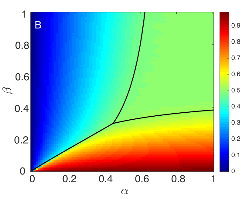
Figure S1: Typical phase diagram and associated simulation. (A) Monte-Carlo simulations as detailed in the text showing the temporal evolution of protein copy number. Averages over 5,000 realizations of stochastic simulations (black lines), twenty example realizations (grey lines), single example trajectory (green line). Red dashed lines are mean field $N^{\ast}$ as computed using the steady state theory. $L=500$ sites, $r=0.005$, $I=0.05$, $k=0.4$, and $n=1$. (B) Monte-Carlo simulations showing the average density of ribosomes, $\rho$, on the mRNA depending on $\alpha$ and $\beta$. 5000 simulations were used for each representative $(\alpha,\beta)$- pair. The black lines show the analytical mean-field phase boundaries derived above.

5 Dynamics in the Modified TASEP

5.1 Onset of oscillations is characterised by a Hopf Bifurcation

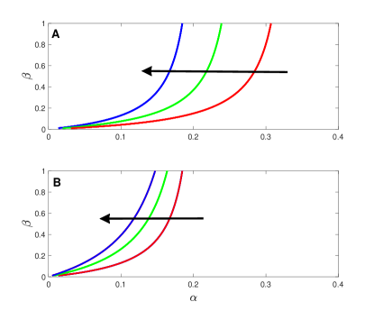
Figure S2: The Hopf locus and the effect of varying recycling and feedback. Hopf bifurcation locus in the $\alpha-\beta$ plane computed using (S34). The effect of varying feedback intensity (A) and recycling (B) is shown. Black arrows indicate direction of increasing effect. (A) $I=10/4$ (blue), $I=10/6$ (green), $I=25/9$ (red) with $k=0.2$ (B) $k=0.6$ (red), $k=0.4$ (blue), $k=0.2$ (red) with $I=10/4$. $L=500$ sites, $r=0.002$, $k=0.2$, $n=5$.

The mean time for a particle to transit the lattice can be estimated as

$$T=\frac{L}{1-\langle\rho\rangle}=\frac{L}{1-\langle\alpha_{eff}\rangle}$$ (S28)

in the LD regime. After substitution and some rearranging, the effective ribosome binding rate in LD is

$$\alpha_{eff}(N)=\dfrac{\alpha(\beta+k)}{\alpha k+\beta\left(1+\left(N/\theta\right)^{n}\right)}.$$ (S29)

Appealing to the mean field approximation and setting $\langle N\rangle=N^{*}$, the mean transit time is then defined as

$$\langle T\rangle=\frac{L}{1-\frac{\alpha(\beta+k)}{\alpha k+\beta\left(1+\left(\frac{\langle N\rangle}{\theta}\right)^{n}\right)}}.$$

The delay differential equation for protein copy number in the LD regime is:

$$\dfrac{dN(t)}{dt}=\dfrac{\alpha(\beta+k)}{\alpha k+\beta\left(1+\left(\dfrac{N(t-T)}{\theta}\right)^{n}\right)}\left(1-\dfrac{\alpha(\beta+k)}{\alpha k+\beta\left(1+\left(\dfrac{N(t-T)}{\theta}\right)^{n}\right)}\right)-rN(t),$$ (S30)

where we have written $T$ for $\langle T\rangle$ for ease of exposition here and below. Steady states, $N^{\ast}$, of (S30) are exactly the solutions generated by substituting solutions of (S20) into the definition $N^{*}=\alpha_{eff}(1-\alpha_{eff})/r$.

To check the stability of $N^{\ast}$, we consider perturbations, $\delta(t)$, with $|\delta|\ll 1$. Substituting $N(t)=N^{\ast}+\delta(t)$ into (S30), using Taylor expansion and dropping the higher order term yields

$$\dfrac{d\delta(t)}{dt}=-B(N^{*})\delta(t-T)-r\delta(t),$$ (S31)

where

$$B(N^{*}):=\left(1-\dfrac{2\alpha(\beta+k)}{\alpha k+\beta\left(1+\left(\dfrac{N}{\theta}\right)^{n}\right)}\right)\dfrac{\alpha\beta(\beta+k)n\left(\dfrac{N}{\theta}\right)^{n}}{N\left(\alpha k+\beta\left(1+\left(\dfrac{N}{\theta}\right)^{n}\right)\right)^{2}}>0$$ (S32)

as $\alpha_{eff}<1/2$ in the LD phase by definition. Setting $\delta(t)=Ae^{\lambda t}$ and on substitution into (S31), we get (hereon setting $B(N^{*})=B$ for ease of notation)

$$\lambda+r=-Be^{-\lambda T}.$$ (S33)

Setting $\lambda=\mu+i\omega$, standard arguments yield a critical wave number at which stability is lost, namely, $\omega^{2}=B^{2}-r^{2}$ and hence a necessary condition is $B>r$. Some algebra eliminates $\omega$ to defines the Hopf locus in terms of system parameters thus:

$$B\cos\left(\sqrt{B^{2}-r^{2}}\,T\right)+r=0.$$ (S34)

Hence, the existence of periodic solutions to (S30) is guaranteed, at least for values of $(\alpha,\beta)$ sufficiently close to the locus. The Hopf locus in the $\alpha-\beta$ plane is shown in Figure SS4 along with the effects of varying $I$ and $k$ (Figs. S3 A and B). Finally, note that the necessary condition $B-r>0$, yields:

$$\dfrac{\alpha\beta(\beta+k)}{\left(\alpha k+\beta\left(1+\left(\dfrac{N^{\ast}}{\theta}\right)^{n}\right)\right)^{3}}g\left(\left(\dfrac{N^{\ast}}{\theta}\right)^{n}\right)>0,$$

where

$$g\left(\left(\dfrac{N^{\ast}}{\theta}\right)^{n}\right)= \beta(n-1)\left(\dfrac{N^{\ast}}{\theta}\right)^{2n}-(\beta+\alpha k)(1-\alpha)$$

$$+\left(\beta(\alpha+n-2\alpha n-2)-(n+1)\alpha k\right)\left(\dfrac{N^{\ast}}{\theta}\right)^{n}.$$ (S35)

Hence, $B-r>0\implies g\left(\left(\dfrac{N^{\ast}}{\theta}\right)^{n}\right)>0$. Notice that if $n=1$, $g\left(\left(\dfrac{N^{\ast}}{\theta}\right)^{n}\right)=\left(-(\alpha+1)\beta-2\alpha k\right)\dfrac{N^{\ast}}{\theta}-(\beta+\alpha k)(1-\alpha)<0$. Hence the Hopf bifurcation cannot occur in this case. Therefore, co-operativity is a necessary condition for Hopf bifurcation to occur.

For $n>1$, the discriminant of $g\left(\left(\dfrac{N^{\ast}}{\theta}\right)^{n}\right)$ is given by:

$$\Delta=\left(\beta(\alpha+n-2\alpha n-2)-(n+1)\alpha k\right)^{2}+4\beta(n-1)(\beta+\alpha k)(1-\alpha),$$ (S36)

and $\Delta>0$ certainly when $\alpha<1$. Therefore, in this case $g\left(\left(\dfrac{N^{\ast}}{\theta}\right)^{n}\right)=0$ has two distinct real roots:

$$\left(\dfrac{N^{\ast}}{\theta}\right)^{n}_{\pm}=\dfrac{-\left(\beta(\alpha+n-2\alpha n-2)-(n+1)\alpha k\right)\pm\sqrt{\Delta}}{2\beta(n-1)},$$

where $\Delta$ is given in (S36) and $\left(\dfrac{N^{\ast}}{\theta}\right)^{n}_{-}$ is negative. Hence, it is easy to conclude that $g\left(\left(\dfrac{N^{\ast}}{\theta}\right)^{n}\right)>0$ requires:

$$\left(\dfrac{N^{\ast}}{\theta}\right)^{n}>\left(\dfrac{N^{\ast}}{\theta}\right)^{n}_{+}=\dfrac{-\left(\beta(\alpha+n-2\alpha n-2)-(n+1)\alpha k\right)+\sqrt{\Delta}}{2\beta(n-1)}.$$ (S37)

The inequality (S37) and setting the right hand side of (S30) to zero, together imply

$$\theta r<\dfrac{\alpha(\beta+k)}{\alpha k+\beta\left(1+\left(\dfrac{N^{\ast}}{\theta}\right)^{n}_{+}\right)}\left(1-\dfrac{\alpha(\beta+k)}{\alpha k+\beta\left(1+\left(\dfrac{N^{\ast}}{\theta}\right)^{n}_{+}\right)}\right)\dfrac{1}{\sqrt[n]{\left(\dfrac{N^{\ast}}{\theta}\right)^{n}_{+}}}.$$ (S38)

Rewriting this in terms of the Intensity Factor $I$ yields the condition $I>F(\bf{\Lambda})$ where $F(\bf{\Lambda})$ is a multiple of the reciprocal of the right hand side of (S38).

5.2 Numerical Simulations of the Characteristic DDE

The DDE (S30) was solved numerically using the code Matlab dde. Typical behaviour for a range of values of $\alpha$ is shown in the Figures below.

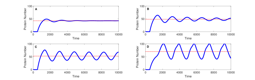
Figure S3: Onset of periodic oscillations in DDE simulation. Solutions of DDE (S30) showing onset of periodic solutions as $\alpha$ is increased through the Hopf locus shown in Figure S4. Blue lines show the numerical solution of (S30). The red dotted line shows the steady state value $N^{*}$ as predicted by the steady state theory. (A) $\alpha=0.1$, (B) $\alpha=0.15$, (C) $\alpha=0.2$, (D) $\alpha=0.8$. Otherwise $L=500$ sites, $\theta=50$, $r=0.002$, $k=0.2$, $n=5$, $\beta=0.5$.

The amplitude and period of the oscillations generated by (S30) are in good agreement with those generated by Monte-Carlo simulations (cf. Fig. S3D and Fig.2A in the main text).

5.3 Periodic oscillations are restricted to the LD Phase

Figure S4: Periodicity in the Monte-Carlo simulations quantified by the autocorrelation function (heat map) compared to the Hopf bifurcation locus in the $\alpha-\beta$ plane analytically calculated using (S34) (upper black curve) and the LD/HD boundary from the mean-field approach (lower black curve). Heatmap shows an autocorrelation-based measure to numerically detect oscillations in the time series of the number of proteins. In particular, we plot the value of the autocorrelation function $ACF(\tau)$ at the first maximum for $\tau>0$. For a maximum to be “well-defined”, the autocorrelation function must cross the horizontal axis twice. If there is no well-defined maximum, we set the measure equal to $0$. Hence, large values (red) in the heatmap indicate pronounced oscillations in the number of proteins. $I=10/4$, $L=500$ sites, $r=0.002$, $k=0.2$, $n=5$.

In the MC phase, $J\equiv 1/4$ and $\alpha_{eff}$ is given by (S15) and thus the loading rate is independent of time. Therefore $N\equiv 1/4r$ is the unique asymptotic solution related to any non-zero initial data. Similarly, in the HD phase, $J=\beta_{eff}(1-\beta_{eff})$, with $\beta_{eff}$ given by the solutions of (S24). In this case, $\beta_{eff}=\beta_{eff}(N(t))$ and thus $J=J(N(t))$ and the characteristic equation $dN/dt=J-rN$ is a scalar, ordinary differential equation with constant coefficients. Standard theory precludes periodic solutions. The behaviour of the characteristic equations therefore supports the numerical simulations to suggest that (almost) periodic solutions are only realised in the LD phase.

We computed an autocorrelation function based measure $ACF(\tau):=E[(N(t)-\mu)(N(t+\tau)-\mu)]/\sigma^{2}$, where $\mu$ is the average and $\sigma$ the standard deviation of the time series $N(t)$ of the number of proteins. $N(t)$ means the time series at time $t$, and $N(t+\tau)$ the time series at time $t+\tau$. Results show that the Hopf locus associated with the DDE provides a reasonable approximation for the parameter region in the $\alpha-\beta$ plane for which oscillations are observed (Fig. S4).

6 Bistability

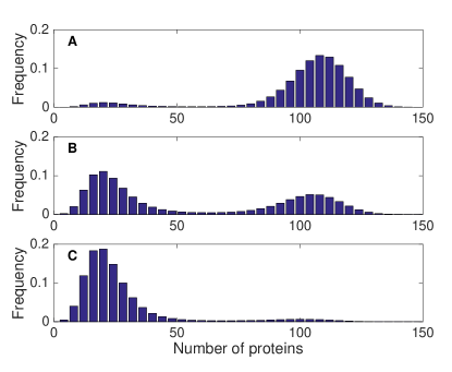
Figure S5: Histograms of the time series of the number of proteins in the bistable state for $L=500$ sites, $\theta=21$, $d=0.002$, $k=0.8$, $\beta=0.015$ and $n=2$ and three different values of $\alpha$: (A) $\alpha=0.75$, (B) $\alpha=0.77$ and (C) $\alpha=0.79$.

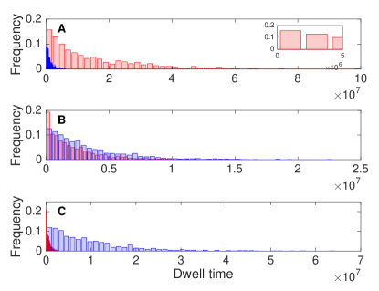
Figure S6: Histograms of the dwell times in each of the bistable states, calculated from the time series of the number of proteins in the bistable region, for $L=500$ sites, $\theta=21$, $d=0.002$, $k=0.8$, $\beta=0.015$ and $n=2$ and three different values of $\alpha$: (A) $\alpha=0.75$, (B) $\alpha=0.77$ and (C) $\alpha=0.79$. The red bars indicate the histogram of the dwell times in the upper stable state, and the blue bars the histogram of the dwell times in the lower stable state. The inset in panel (A) shows a zoom of the histogram for the upper stable state for low dwell times, to demonstrate that the smallest dwell times are larger than $0$.

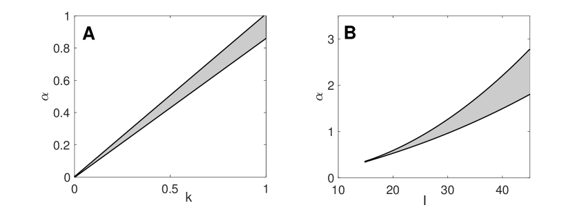
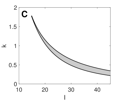
Figure S7: Regions of bistability as predicted by the steady state theory shown as functions of feedback ($I$), recycling ($k$) and loading rates ($\alpha$). Bistable regions are shaded grey. (A) $\alpha$-$I$ plane ($k=0.8$) (B) $\alpha$-$k$ plane ($I=24$) (C) $I$-$k$ plane ($\alpha=0.77$). Otherwise $L=500$, $n=2$, $\beta=0.015$.