A stochastic partial differential equation model for limit order book dynamics

Abstract.

We propose an analytically tractable class of models for the dynamics of a limit order book, described through a stochastic partial differential equation (SPDE) with multiplicative noise for the order book centered at the mid-price, along with stochastic dynamics for the mid-price which is consistent with the order flow dynamics. We provide conditions under which the model admits a finite dimensional realization driven by a (low-dimensional) Markov process, leading to efficient estimation and computation methods. We study two examples of parsimonious models in this class: a two-factor model and a model with mean-reverting order book depth. For each model we analyze in detail the role of different parameters, the dynamics of the price, order book depth, volume and order imbalance, provide an intuitive financial interpretation of the variables involved and show how the model reproduces statistical properties of price changes, market depth and order flow in limit order markets.

 

Financial instruments such as stocks and futures are increasingly traded in electronic, order-driven markets, in which orders to buy and sell are centralized in a limit order book and market orders are executed against the best available offers in the limit order book. The dynamics of prices in such markets are not only interesting from the viewpoint of market participants –for trading and order execution– but also from a fundamental perspective, since they provide a detailed view of the dynamics of supply fand demand and their role in price formation.

The availability of a large amount of high frequency data on order flow, transactions and price dynamics on these markets has instigated a line of research which, in contrast to traditional market microstructure models which make assumptions on the behavior and preferences of various types of agents, focuses on the statistical modeling of aggregate order flow and its relation with price dynamics, in a quest to understand the interplay between price dynamics and order flow of various market participants [Cont, 2011].

A fruitful line of approach to these questions has been to model the stochastic dynamics of the limit order book, which centralizes all buy and sell orders, either as a queueing system [Luckock, 2003, Smith et al., 2003, Cont et al., 2010, Cont and De Larrard, 2012, Cont and de Larrard, 2013, Kelly and Yudovina, 2018] or, at a coarse-grained level, through a (stochastic) partial differential equation describing the evolution of the distribution of buy and sell orders [Lasry and Lions, 2007, Caffarelli et al., 2011, Burger et al., 2013, Carmona and Webster, 2013, Markowich et al., 2016, Hambly et al., 2020, Horst and Kreher, 2018]. These PDE models may be viewed as scaling limits of discrete point process models [Cont and De Larrard, 2012, Hambly et al., 2020, Horst and Kreher, 2018].

Although joint modeling of order flow at all price levels in the limit order book is more appealling, (S)PDE models have lacked the analytical and computational tractability needed for applications; as a result, most analytical results have been derived using reduced-form models of the best bid-ask queues [Cont and De Larrard, 2012, Cont and de Larrard, 2013, Chavez-Casillas and Figueroa-Lopez, 2017, Huang et al., 2017].

We propose a class of stochastic models for the dynamics of the limit order book which represent the dynamics of the entire order book while retaining at the same time the analytical and computational tractability of low-dimensional Markovian models, and provides realistic dynamics for the joint dynamics of the market price and order book depth. Starting with a description of the dynamics of the limit order book via a stochastic partial differential equation (SPDE) with multiplicative noise, we show that in many cases, the solutions of this equation may be parameterized in terms of a low-dimensional diffusion process, which then makes the model computationally tractable. In particular, we are able to derive analytical relations between model parameters and various observable quantities. This feature may be used for calibrating model parameters to match statistical features of the order flow and leads to empirically testable predictions, which we proceed to test using high frequency time series of order flow in electronic equity markets.

Outline Section 1 introduces a description of the dynamics of a limit order book through a stochastic partial differential equation (SPDE). We describe the various terms in the equation, their interpretation and discuss the implications for price dynamics (Section 1.3). This class of models is part of a more general family of SPDEs driven by semimartingales, introduced in Sec. 1.5 and studied in Sec. 2.

We then focus on two analytically tractable examples: a two-factor model (Section 3) and a model with mean-reverting depth and imbalance (Section 4). For each model we perform a detailed analysis of the role of different parameters and study the dynamics of the price, order book depth, volume and order imbalance, provide an intuitive financial interpretation of the variables involved and show how the model may be estimated from financial time series of price, volume and order flow.

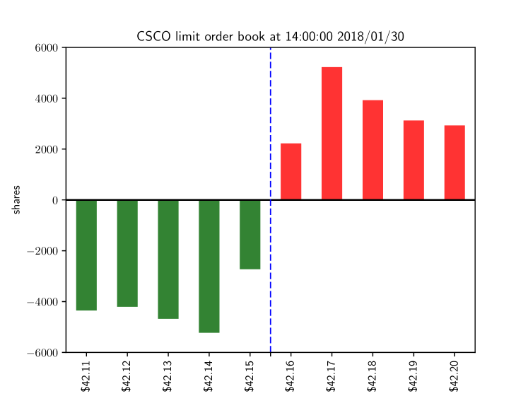
Figure 1. Snapshot of the NASDAQ limit order book for CISCO shares (Jan 30, 2018), displaying outstanding buy orders (green) and sell orders (red) awaiting execution at different prices. The highest buying price ($ 42.15 in this example) is the bid and the lowest selling price ($ 42.16) is the ask.

1. A stochastic PDE model for limit order book dynamics

We consider a market for a financial asset (stock, futures contract, etc.) in which buyers and sellers may submit limit orders to buy or sell a certain quantity of the asset at a certain price, and market orders for immediate execution against the best available price. Limit orders awaiting execution are collected in the limit order book, an example of which is shown in Figure 1: at any time $t$, the state of the limit order book is summarized by the volume $V(t,p)$ of orders awaiting execution at price levels $p$ on a grid with mesh size given by the minimum price increment or tick size $\delta$. By convention we associate negative volumes with buy orders and positive volumes with sell orders, as shown in Figure 1. An admissible order book configuration is then represented by a function $p\mapsto V(p)$ such that

$$0<s^{b}(V):=\sup\{p>0,\quad V(p)<0\}\leq s^{a}(V):=\inf\{p>0,\quad V(p)>0\}<\infty.$$

$s^{b}(V)$ (resp. $s^{a}(V)$) is called the bid (resp. ask) price and represents the price associated with the best buy (resp. sell) offer. The quantity

$$S=\frac{s^{a}(V)+s^{b}(V)}{2}$$

is called the mid-price and the difference $s^{a}(V)-s^{b}(V)$ is called the bid-ask spread. In the example shown in Figure 1, $s^{b}(V)=42.15,s^{a}(V)=42.16$ and the bid-ask spread is equal in this case to the tick size, which is 1 cent.

One modelling approach has been to represent the dynamics of $V(t,p)$ as a spatial (marked) point process [Luckock, 2003, Cont et al., 2010, Cont and de Larrard, 2013, Kelly and Yudovina, 2018]. These models preserve the discrete nature of the dynamics at high frequencies but can become computationally challenging as one tries to incorporate realistic dynamics. In particular, price dynamics, which is endogenous in such models, is difficult to study, even when the order flow is a Poisson point process.

When the bid-ask spread and tick size $\delta$ are much smaller than the price level, as is often the case, another modelling approach is to use a continuum approximation for the order book, describing it through its density $v(t,p)$ representing the volume of orders per unit price:

$$V(t,p)\simeq v(t,p)\delta.$$

The evolution of the density of buy and sell orders is then described through a partial differential equation (PDE). A deterministic description of the dynamics of order densities through a system of coupled partial differential equations was proposed by [Lasry and Lions, 2007] and studied in detail by [Chayes et al., 2009, Caffarelli et al., 2011, Burger et al., 2013]. In the Lasry-Lions model, the evolution of the density of buy and sell orders is described by a pair of diffusion equations coupled through the dynamics of the price, which represents the free boundary between prices of buy and sell orders. This model is appealing in many respects, especially in terms of analytical tractability, but leads to a deterministic price process which decays to a constant price, so does not provide any insight into the relation between liquidity, depth, order flow and price volatility. [Markowich et al., 2016] explore some stochastic extensions of this model but essentially show that these extensions do not provide realistic price dynamics.

We adopt here this continuum approach for the description of the limit order book, but describe instead its dynamics through a stochastic partial differential equation, paying close attention to price dynamics and its relation with order flow.

The model we propose shares some features with [Lasry and Lions, 2007], but also has some essential differences. Unlike the Lasry-Lions model, which is a free boundary problem in which the dynamics of the price is implicitly determined, we formulate the model as a stochastic partial differential equation in relative price coordinates, which leads to a stochastic moving boundary problem in absolute price coordinates. This leads to a more realistic joint dynamics for the market price and order book depth which can be related to empirical observations. Our model also relates to the classes of models studied in [Horst and Kreher, 2018, Hambly et al., 2020] as scaling limits of discrete queueuing systems.

We now describe our model in some detail.

1.1. State variables and scaling transformations

We focus on the case where the tick size $\delta$ and the bid-ask spread are small compared to the typical price level and consider a limit order book described in terms of a mid-price $S_{t}$ and the density $v(t,p)$ of orders at each price level $p$, representing buy orders for $p<S_{t}$, and sell orders for $p>S_{t}$. We use the convention, shown in Figure 1, of representing buy orders with a negative sign and sell orders with a positive sign, so

$$v(t,p)\leq 0\quad{\rm for}\quad p<S_{t}\quad{\rm and}\quad v(t,p)\geq 0\quad{\rm for}\quad p>S_{t}$$

Limit orders are executed against market orders according to price priority and their position in the queue; execution of a limit order only occurs if they are located at the best (buy/sell) prices. This means that price dynamics is determined by the interaction of market orders with limit orders of opposite type at or near the interface defined by the best price [Cont et al., 2010]. Due to this fact, most limit orders flow are submitted close to the best price levels: the frequency of limit order submissions is highly inhomogeneous as a function of distance to the best price and concentrated near the best price. As shown in previous empirical studies, order flow intensity at a given distance from the best price can be considered as a stationary variable in a first approximation [Bouchaud et al., 2009, Cont et al., 2010]. For this reason, in a stochastic description it is more convenient to model the dynamics of order flow in the reference frame of the (mid-)price $S_{t}$. We define

$$u_{t}(x)=v(t,S_{t}+x)$$

where $x$ represents a distance from the mid-price. We refer to $u_{t}$ as the centered order book density.

The simplest way of centering is to set $x(p)=p-S_{t}$ but other, nonlinear, scalings may be of interest. Although limit orders may be placed at any distance from the bid/ask prices, price dynamics is dominated by the behavior of the order book a few levels above and below the mid price [Cont and De Larrard, 2012]. This region becomes infinitesimal if the tick size $\delta$ is naively scaled to zero, suggesting that the correct scaling limit is instead one in which we choose as coordinate a scaled version $(p-S_{t})$, as classically done in boundary layer analysis of PDEs [Schlichting and Gersten, 2017], in order to zoom into the relevant region:

(1.1) $$x(p):=-(S_{t}-p)^{a},\quad p<S_{t},\qquad x(p)=(p-S_{t})^{a},\quad p>S_{t},\qquad a>0$$

for bid and ask side, respectively. We will consider examples of such nonlinear scalings when discussing applications to high-frequency data in Sections 3 and 4.

These arguments also justify limiting the range of the argument $x$to a bounded interval $[-L,+L]$, setting $u_{t}(x)=0$ for $x\notin(-L,L)$. This amounts to assuming that no orders are submitted at price levels at distances $|x|\geq L$ from the mid-price and that orders previously submitted at some price $p$ are cancelled as soon as $|S_{t}-p|\geq L$ i.e. when the mid-price $S_{t}$ moves away from $p$ by more than $L$. When $L$ is a large multiple of daily volatility, this is a realistic assumption. In some market (for example futures contracts), limit orders can be in fact only submitted within a range $\pm L$ of the mid-price.

1.2. Dynamics of the centered limit order book

Empirical studies on intraday order flow in electronic markets reveal the coexistence of two, very different types of order flow operating at different frequencies [Lehalle and Laruelle, 2018].

On one hand, we observe the submission (and cancellation) of orders queueing at various price levels on both sides of the market price by regular market participants. Cancellation may occur in several ways: we distinguish outright cancellations, which we model as proportional to current queue size, from cancellations with replacement (‘order modifications’), in which an order is cancelled and immediately replaced by another one of the same type, usually at a neighboring price limit. The former results in a net decrease in the volume of the order book whereas the latter is conservative and simply shifts orders across neighboring levels of the book. Further decomposing this conservative flow into a symmetric and antisymmetric part leads to two terms in the dynamics of $u_{t}$: a diffusion term representing the cancellation of orders and their (symmetric) replacement by orders at neighboring price levels and a convection (or transport) term representing the cancellation of orders and their replacement by orders closer to the mid-price. Denoting by $\nabla$ the gradient in the variable $x$, the net effect of this order flow on the order book may thus be described as a superposition of

• a term $f^{b}(x)$ (resp. $f^{a}(x)\ )$ representing the rate of buy (resp. sell) order submissions at a distance $x$ from the best price;

• a term $\alpha_{b}\ u_{t}(x)$ (resp. $\alpha_{a}\ u_{t}(x)$) representing (outright) proportional cancellation of limit buy (resp. sell) orders at a distance $x$ from the mid-price (where $\alpha_{a},\alpha_{b}\leq 0$).

• a convection term $-\beta_{b}\nabla u_{t}(x)$ (resp. $+\beta_{a}\nabla u_{t}(x)$) with $\beta_{a},\beta_{b}>0$ which models the replacement of buy (resp. sell) orders by orders closer to the mid-price (i.e. closer to $x=0$, hence the signs in these terms): in the reference frame where the origin is the mid-price, this translates into a flow of volume towards the origin;

• a diffusion term $\eta_{b}\Delta u_{t}(x)$ (resp. $\eta_{a}\Delta u_{t}(x)$) which represents the cancellation and symmetric replacement of orders at a distance $x$ from the mid-price.

Another component of order flow is the one generated by high-frequency traders (HFT). These market participants buy and sell at very high frequency and under tight inventory constraints, submitting and cancelling large volumes of limit orders near the mid-price and resulting in an order flow whose net contribution to total order book volume is zero on average over longer time intervals but whose sign over small time intervals fluctuates at high frequency. At the coarse-grained time scale of the average (non-HF) market participants, these features may be modeled as a multiplicative noise term of the form

• $\sigma_{b}u_{t}(x)dW^{b}$ for buy orders ($x<0$) and $\sigma_{a}u_{t}(x)dW^{a}$ for sell orders ($x>0$)

where $(W^{a},W^{b})$ is a two-dimensional Wiener process (with possibly correlated components). The multiplicative nature of the noise accounts for the high-frequency cancellations associated with HFT orders.

The impact of these different order flow components may be summarized by the following stochastic partial differential equation for the centered order book density $u$:

$$\,\operatorname{d}u_{t}(x) =\left[\eta_{a}\Delta u_{t}(x)+\beta_{a}\nabla u_{t}(x)+\alpha_{a}u_{t}(x)+f^{a}(x)\right]\,\operatorname{d}t+\sigma_{a}u_{t}(x)\,\operatorname{d}W^{a}_{t},\quad\,x\in(0,L),$$

(1.2) $$\,\operatorname{d}u_{t}(x) =\left[\eta_{b}\Delta u_{t}(x)-\beta_{b}\nabla u_{t}(x)+\alpha_{b}u_{t}(x)-f^{b}(x)\right]\,\operatorname{d}t+\sigma_{b}u_{t}(x)\,\operatorname{d}W^{b}_{t},\quad\,x\in(-L,0)$$

$$u_{t}(x)\leq 0,\quad x<0,\qquad\quad\;u_{t}(x)\geq 0,\quad x>0,$$

$$u_{t}(0+)=u_{t}(0-)=0,\qquad u_{t}(-L)=u_{t}(L)=0$$

Here $\eta_{a}$, $\eta_{b}$, $\beta_{b}$, $\beta_{a}$, $\sigma_{a}$, $\sigma_{b}\in(0,\infty)$, $\alpha_{a},\alpha_{b}\leq 0$ and $f^{a}$, $f^{b}\colon I\to[0,\infty)$ although the equation may be equally considered without these sign restrictions.

Note that, unlike the Lasry-Lions model, there is no ‘smooth pasting’ condition at $x=0$: in general $\nabla u_{t}(0+)\neq\nabla u_{t}(0-)$: the difference $\nabla u_{t}(0+)-\nabla u_{t}(0-)$ is in fact random and represents an imbalance in the flow of buy and sell orders, which drives price dynamics. This important feature is discussed in Section 1.3 below.

Remark 1.1.

In simple price impact models used in the literature on optimal trade execution it is assumed that the relation between price impact and order size is deterministic. This corresponds to the case $\alpha u+f=\beta=\sigma=\eta=0$ which leads to a constant centered order book profile $u_{t}(.)=u_{0}(.)$. These terms thus correspond to deformations of the centered order book profile due to new order book events and lead to a stochastic market impact of trades dependent on the current state of the order book.

The existence of a solution satisfying the boundary and sign constraints is not obvious but we will see in Section 2 that (1.2) is well-posed: it follows from [Da Prato and Zabczyk, 2014, Theorem 6.7] and [Milian, 2002, Theorem 3] that, when $f_{a}$, $f_{b}\in L^{2}(I)$, then for all $u_{0}\in L^{2}(I)$ there exists a unique weak solution of (1.2) (see Definition 2.2 below) and, when $u_{0}|_{(0,L)}\geq 0$ and $u_{0}|_{(-L,0)}\leq 0$ this solution satisfies

(1.3) $$u_{t}|_{(0,L)}\leq 0,\qquad u_{t}|_{(-L,0)}\geq 0.$$

We will study the mathematical properties of the solution in more detail below.

1.3. Price dynamics

The dynamics of the limit order book determines the dynamics of the bid and ask price, which corresponds to the location of the best (buy and sell) orders. The dynamics of the price should thus be related to the arrival and execution of orders in the order book.

To understand the relation between price dynamics and order flow, let us take a step back and consider an order book with discrete price levels, multiples of a tick size $\delta$, $D^{b}$ orders per level on the bid side and $D^{a}$ orders per level on the ask side. Price changes during a time interval $[t,t+\Delta t]$ are triggered through the interaction of the net order flow, or order flow imbalance (OFI) and the outstanding limit orders at the top of the order book [Cont et al., 2014]. As illustrated in Figure 2, an order flow imbalance of $\Delta D^{a}_{t}>0$ on the ask side over a short time interval $[t,t+\Delta t]$ represents an excess of buy orders, which will then be executed against limit sell orders sitting on the ask side and move the ask price by $\Delta D^{a}_{t}/D^{a}$ ticks, resulting in a price move of $\delta\ \Delta D^{a}_{t}/D^{a}$. Similarly, an order flow imbalance $\Delta D^{b}_{t}$ on the bid side will move the bid price up by $\Delta D^{b}_{t}/D^{b}$ ticks. Using our sign conventions for buy/sell volumes, this leads to the following dynamics:

$$\Delta s^{b}_{t}=\delta\frac{\Delta D_{t}^{b}}{D^{b}_{t}}\qquad\Delta s^{a}_{t}=-\delta\frac{\Delta D_{t}^{a}}{D^{a}_{t}},$$

so the dynamics of the mid price $s_{t}=(s^{b}_{t}+s^{a}_{t})/2$ is given by

(1.4) $$\Delta S_{t}=\frac{\delta}{2}\left(\frac{\Delta D_{t}^{b}}{D^{b}_{t}}-\frac{\Delta D_{t}^{a}}{D^{a}_{t}}\right).$$

This relation is exact (up to rounding) in the case of a discrete order book with constant depth per level (and thus, no empty levels), as shown in Figure 2. However, in a dynamic setting where the order book may have an arbitrary profile which randomly shifts at each instant, one can only expect a ‘homogenized’ version of (1.4) to hold:

(1.5) $$\Delta S_{t}={\theta}\left(\frac{\Delta D_{t}^{b}}{D^{b}_{t}}-\frac{\Delta D_{t}^{a}}{D^{a}_{t}}\right)$$

where $\theta$ is an impact coefficient which relates order imbalance to price movements. This relation between order flow imbalance and price movements has been empirically verified in equity markets [Cont et al., 2014], and we shall use it as a basis for defining the relation between price dynamics and order flow in our model.

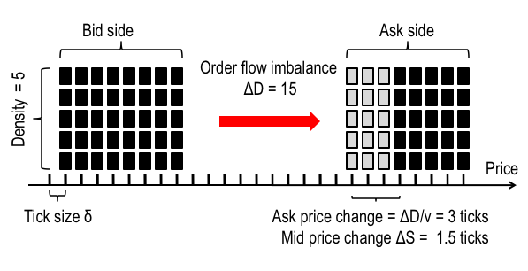
Figure 2. Impact of order flow imbalance on the order book and the price.

Let us now see how the relation (1.5) translates in terms of the variables in our model. Denoting by $D^{b}_{t}$ (resp. $D^{a}_{t}$) the volume of buy (resp. sell) limit orders at the top of the book (i.e. the first or average of the first few levels). Given a mid-price $S\in\mathbb{R}_{+}$, we define a scaling transformation $x\colon[S,S+L]\to[0,\infty)$ as discussed in Section 1.1, with continuously differentiable inverse and such that $x(S)=0$. The volume $D^{a}$ in the best ask queue is then given by

(1.6) $$D^{a}=\int_{s}^{s+\delta}u(x(p))\,\operatorname{d}p=\int_{0}^{x(s+\delta)}u(y)(x^{-1})^{\prime}(y)\,\operatorname{d}y.$$

$D^{b}$ may be similarly defined for the bid side. These quantities represent the depth at the top of the book; we will refer to them as ‘market depth’. In the case of linear scaling $x(p)=p-S$, using $u(0)=0$ a second order expansion in $\delta>0$ yields

(1.7) $$D^{a}=\int_{0}^{\delta}u(x)\,\operatorname{d}x\approx\delta u(0+)+\frac{\delta^{2}}{2}\nabla u(0+)=\frac{\delta^{2}}{2}\nabla u(0+).$$

Similarly, for the bid side

(1.8) $$D^{b}\approx\frac{\delta^{2}}{2}\nabla u\left(0-\right).$$

Substituting these expressions in (1.5), we obtain the following dynamics of the mid-price:

(1.9) $$\,\operatorname{d}S_{t}=\theta\left(\frac{\,\operatorname{d}D^{b}_{t}}{D_{t}^{b}}-\frac{\,\operatorname{d}D^{a}_{t}}{D_{t}^{a}}\right)=\theta\left(\frac{\,\operatorname{d}\nabla u_{t}(0-)}{\nabla u_{t}(0-)}-\frac{\,\operatorname{d}\nabla u_{t}(0+)}{\nabla u_{t}(0+)}\right).$$

We observe that price dynamics is entirely determined by the order flow at the top of the book and the depth of the limit order book around the mid-price. The tick size $\delta$, used in the derivation, does not appear anymore in (1.9). The only trace of the microstructure is the impact coefficient $\theta$ which relates the order flow imbalance to the magnitude of the price change, and whose amplitude may vary across assets.

Remark 1.2.

Equation (1.9) requires left and right-differentiability of $u$ at the origin. This can be guaranteed whenever $u_{t}$ takes values in the Sobolev space $H^{2\gamma}(I)$, for some $\gamma>\nicefrac{{3}}{{4}}$ which will be the case in our model. Note however that, in contrast to [Lasry and Lions, 2007], in general $\nabla u(0+)\neq\nabla u(0-)$: the difference between these two quantities is proportional to the order flow imbalance which drives price moves.

Remark 1.3.

As noted in Remark 1.1, in the case $\alpha u+f=\beta=\sigma=\eta=0$ corresponds to a constant centered order book profile $u_{t}=u_{0}$. In this case, Equation (1.9) implies $dS_{t}=0$ i.e. the price is constant, which is consistent with a zero net order flow. This is a (desirable) consequence of the consistency between the price dynamics (1.9) and the order book dynamics (1.2).

1.4. Dynamics in absolute price coordinates

The model above describes dynamics of the order book in relative price coordinates, i.e. as a function of the (scaled) distance from the mid-price. The density of the limit order book parameterized by the (absolute) price level $p\in\mathbb{R}$ is given by

(1.10) $$v_{t}(p)=u_{t}(p-S_{t}),\qquad x\in\mathbb{R},$$

where we extend $u_{t}$ to $\mathbb{R}$ by setting $u_{t}(y)=0$ for $y\in\mathbb{R}\setminus[-L,L]$. Assume $S_{t}$ follows an (arbitrary) Itô process

$$\,\operatorname{d}S_{t}=\theta\mu_{t}\,\operatorname{d}t+\theta\xi_{t}^{b}\,\operatorname{d}W_{t}^{b}-\theta\xi_{t}^{a}\,\operatorname{d}W_{t}^{a}$$

where $\theta>0$ and $\mu_{t}$ is predictable and integrable and $\xi_{t}^{a}$ and $\xi_{t}^{b}$ are predictable and square-integrable processes. This includes the case of price dynamics (1.9), which can be used to express $\mu_{t},\xi_{t}^{a},\xi_{t}^{b}$ in terms of $u_{t}$ and model parameters. We will not go into such detail here but will return to this in the examples in Section 3 and 4. Define

$$\hat{\xi}_{t}:=\sqrt{(\xi_{t}^{b})^{2}+(\xi_{t}^{a})^{2}-2\varrho_{a,b}\xi_{t}^{b}\xi_{t}^{a}},\qquad t\geq 0.$$

Using a (generalized) Itô-Wentzell formula (see Appendix A), we can show that $v$ is the solution of a stochastic moving boundary problem [Mueller, 2018]:

(1.11) $$\,\operatorname{d}v_{t}(p)=\left[(\eta_{a}+\tfrac{1}{2}\theta^{2}\hat{\xi}_{t}^{2})\Delta v_{t}(p)\right.\\ \left.+\left(\beta_{a}-\theta\mu_{t}-\theta\sigma_{a}(\varrho_{a,b}\xi_{t}^{b}-\xi_{t}^{a})\right)\nabla v_{t}(p)+\alpha_{a}v_{t}(p)\right]\,\operatorname{d}t\\ +\left(\sigma_{a}v_{t}(p)+\theta\xi_{t}^{a}\nabla v_{t}(p)\right)\,\operatorname{d}W_{t}^{a}-\theta\xi_{t}^{b}\nabla v_{t}(p)\,\operatorname{d}W_{t}^{b},$$

for $p\in(S_{t},S_{t}+L)$, and

(1.12) $$\,\operatorname{d}v_{t}(p)=\left[(\eta_{b}+\tfrac{1}{2}\theta^{2}\hat{\xi}_{t}^{2})\Delta v_{t}(p)\right.\\ \left.+(-\theta\mu_{t}-\beta_{b}-\theta\sigma_{b}(\xi_{t}^{b}-\varrho_{a,b}\xi_{t}^{a}))\nabla v_{t}(x)+\alpha_{b}v_{t}(p)\right]\,\operatorname{d}t\\ +\theta\xi_{t}^{a}\nabla v_{t}(p)\,\operatorname{d}W_{t}^{a}+\left(\sigma_{b}v_{t}(p)-\theta\xi_{t}^{b}\nabla v_{t}(p)\right)\,\operatorname{d}W_{t}^{b}$$

for $x\in(S_{t}-L,S_{t})$ with the moving boundary conditions

(1.13) $$v_{t}(S_{t})=0,\qquad v_{t}(y)=0,\qquad\forall y\in\mathbb{R}\setminus(S_{t}-L,S_{t}+L),$$

We refer to (1.13) as a stochastic boundary condition at $S_{t}$.

Here, we assumed for simplicity that $f^{a}$, $f^{b}=0$. A more detailed discussion of this result is given in Appendix A.

1.5. Linear evolution models for order book dynamics

We will now describe a more general class of linear models for order book dynamics, rich enough to cover the examples we discussed so far, but also covering all level-1 models where the best bid and ask queue are modeled by positive semimartingales. Generally, the densities of orders in the bid and ask side will take values in some function spaces $H^{b}$ and $H^{a}$, respectively. We assume that orders at relative price level $x$ for $\left\lvert x\right\rvert\geq L\in(0,\infty]$ will be cancelled. The relative price levels are on the bid side $I^{b}:=(-L,0)$, and on the ask side $I^{a}:=(0,L)$. Then, in order to preserve the interpretation of a density it will be reasonable to ask $H^{b}\subset L^{1}_{loc}(I^{b})$ and $H^{a}\subset L^{1}_{loc}(I^{a})$. From mathematical side, we will assume that $H^{a}$ and $H^{b}$ are real separable Hilbert spaces. For notational convenience we now also set $I:=I^{b}\cup I^{a}$.

The density of limit orders at relative price level $x$ and time $t$ is given by $u\colon I\times[0,\infty)\times\Omega\to\mathbb{R}$, such that $u^{\star}:=u|_{I^{\star}}$ is an $H^{\star}$-valued adapted process. The initial state is described by $h\colon I\to\mathbb{R}$, such that $h^{\star}:=h|_{I^{\star}}$ is an element in $H^{\star}$. The (averaged) intra-book dynamics are modeled by linear operators $A_{\star}\colon{\rm dom}(A_{\star})\subset H^{\star}\to H^{\star}$, for $\star\in\{a,b\}$, which we assume to be densely defined and such that for $\star\in\{a,b\}$ there exist weak solutions in $H^{\star}$ of the equations

(1.14) $$\tfrac{\partial}{\partial t}g_{t}^{\star}(h^{\star})=A_{\star}g_{t}^{\star}(h^{\star}),\quad t>0,\quad g_{0}^{\star}(h^{\star})=h^{\star},$$

for each initial state $h^{\star}\in H^{\star}$.

The random order arrivals and cancellations are assumed to be proportional and are modelled by cadlag semimartingales $X^{b}$ and $X^{a}$, which we assume to have jumps greater than $-1$ almost surely. We assume the initial order book state is denoted by $h\in H$ and we write $h^{a}:=h|_{I^{a}}$, $h^{b}:=h|_{I^{b}}$.

Model 1.4 (Linear Homogeneous Evolution).

The general form of the linear homogeneous model is

(1.15) $$\left\{\begin{aligned} \,\operatorname{d}u_{t}^{b}&=A_{b}u_{t-}^{b}\,\operatorname{d}t+u_{t-}^{b}\,\operatorname{d}X_{t}^{b},\quad&\text{on }&I^{b},\\ \,\operatorname{d}u_{t}^{a}&=A_{a}u_{t-}^{a}\,\operatorname{d}t+u_{t-}^{a}\,\operatorname{d}X_{t}^{a},\quad&\text{on }&I^{a},\end{aligned}\right.$$

for $t\geq 0$, and $u_{0}=h$. $u$ can be alternatively expressed as

(1.16) $$u_{t}=g_{t}^{b}(h^{\star})\mathcal{E}_{t}(X^{b})\mathbf{1}_{I^{b}}+g_{t}^{a}(h^{\star})\mathcal{E}_{t}(X^{a})\mathbf{1}_{I^{a}},$$

where $g^{b}$ and $g^{a}$ are solutions of (1.14), see Theorem 2.5 below. If, in addition, $t\mapsto\nabla g_{t}^{b}(0-)$ and $t\mapsto\nabla g_{t}^{a}(0+)$ are of bounded variation, then we obtain the price dynamics (1.9).

Corollary 1.5.

Assume the setting of Model 1.4 and, in addition, that $h^{\star}$ is an eigenfunction of $-A_{\star}$ with eigenvalue $\nu_{\star}\in\mathbb{R}$, for $\star=b$ and $\star=a$. Then, (1.14) can be solved explicitly and

(1.17) $$u_{t}=h^{b}e^{-\nu_{b}t}\mathcal{E}_{t}(X^{b})\mathbf{1}_{I^{b}}+h^{a}e^{-\nu_{a}t}\mathcal{E}_{t}(X^{a})\mathbf{1}_{I^{a}}.$$

Remark 1.6.

In case that $X^{b}$ and $X^{a}$ are (local) martingales, the eigenvalues $-\nu_{b}$ and $-\nu_{a}$ play the role of net order arrival rates on bid and ask side, respectively.

Model 1.7 (Linear models with source terms).

A more realistic setting assumes in addition an influx/outflow of orders at a rate $f^{a}(x),f^{b}(x)$ which depends on the distance $x$ to the mid price [Cont et al., 2010]. The equation then becomes:

(1.18) $$\left\{\begin{aligned} \,\operatorname{d}u_{t}^{b}&=\left(A_{b}u_{t}^{b}+f^{b}\right)\,\operatorname{d}t+u_{t}^{b}\,\operatorname{d}X_{t}^{b},\quad&\text{on }&I^{b},\\ \,\operatorname{d}u_{t}^{a}&=\left(A_{a}u_{t}^{a}+f^{a}\right)\,\operatorname{d}t+u_{t}^{a}\,\operatorname{d}X_{t}^{a},\quad&\text{on }&I^{a},\end{aligned}\right.$$

for $t\geq 0$, with initial condition $u_{0}=h$.

As we will discuss in Section 4, an interesting case is when $f^{b}$ (resp. $f^{a}$) is an eigenfunction of $-A^{b}$ (resp. $-A^{a}$) associated with some eigenvalue $\nu_{b}$ (resp. $\nu_{a}$). Then by Theorem 2.10 we obtain

(1.19) $$u_{t}=\left(g_{t}^{b}(h^{b}-f^{a})\mathcal{E}_{t}(X^{b})+f^{b}Z_{t}^{b}\right)\mathbf{1}_{I^{b}}+\left(g_{t}^{a}(h^{a}-f^{a})+f^{a}Z_{t}^{a}\right)\mathbf{1}_{I^{a}},$$

where, for $\star\in\{a,b\}$, $Z_{t}^{\star}$ is the solution of

(1.20) $$\,\operatorname{d}Z_{t}^{\star}=(1-\nu_{\star}Z_{t-}^{\star})\,\operatorname{d}t+Z_{t-}^{\star}\,\operatorname{d}X_{t}^{\star},\quad t\geq 0,\quad Z_{0}^{\star}=1.$$

Remark 1.8.

If $\nu_{b}$, $\nu_{a}>0$ the state of the order book is mean reverting to the state $f^{b}1_{[-L,0)}+f^{a}\ 1_{(0,L]}$. We will give an example of such a mean-reverting order book model in Section 4.

Remark 1.9.

Any model for the dynamics of the order book implies a model for price dynamics via (1.9). In particular this implies a relation between price volatility and parameters describing order flow, in the spirit of [Cont and de Larrard, 2013]. We will derive this relation for the examples studied in the sequel and use it to construct a model-based intraday volatility estimator.

In the next section, we will study this class of models from a mathematical point of view. We will then continue with the analysis of the two examples mentioned above in Sections 3 and 4.

2. Linear stochastic PDE models with multiplicative noise

In order to further study the properties of the SPDE model (1.2), we require a more explicit characterization of the solution, in order to compute various quantities of interest and estimate model coefficients from observations. A useful approach is to look for a finite dimensional realization of the infinite-dimensional process $u$:

Definition 2.1 (Finite dimensional realizations).

A process $u=(u_{t})_{t\geq 0}$ taking values in an (infinite-dimensional) function space $E$ is said to admit a finite dimensional realization of dimension $d\in\mathbb{N}$ if there exists an $\mathbb{R}^{d}$-valued stochastic process $Z=(Z^{1},...,Z^{d})$ and a map

$$\phi:\mathbb{R}^{d}\to E\quad{\rm such\ that}\quad\forall t\geq 0,\quad u_{t}=\phi(Z_{t}).$$

Availability of a finite dimensional realization for the SPDE (1.2) makes simulation, computation and estimation problems more tractable, especially if the process $Z$ is a low-dimensional Markov process. Existence of such finite-dimensional realizations for stochastic PDEs have been investigated for SPDEs arising in filtering [Lévine, 1991] and interest rate modelling [Filipovic and Teichmann, 2003, Gaspar, 2006].

We will now show that finite dimensional realizations may indeed be constructed for a class of SPDEs which includes (1.2), and use this representation to perform an analytical study of these models.

2.1. Homogeneous equations

We now consider a more general class of linear homogeneous evolution equations with multiplicative noise taking values in a real separable Hilbert space $(H,\langle\cdot,\cdot\rangle_{H})$. Typically, $H$ will be a function space such as $L^{2}(I)$ for some interval $I\subset\mathbb{R}$. We consider the following class of evolution equations:

(2.1) $$\begin{split}\,\operatorname{d}u_{t}&=Au_{t-}\,\operatorname{d}t+u_{t-}\,\operatorname{d}X_{t},\qquad t>0,\\ u_{0}&=h_{0}\in H.\end{split}$$

where $X$ is a real càdlàg semimartingale whose jumps satisfy $\Delta X_{t}>-1$ a. s. and $A\colon{\rm dom}(A)\subset H\to H$ a linear operator on $H$ whose adjoint we denote by $A^{*}$. We assume that ${\rm dom}(A)\subset H$ is dense, and $A$ is closed. Since $A$ is closed we have that also ${\rm dom}(A^{*})\subset H$ is dense and that $A^{**}=A$ [Yosida, 1995, Theorem VII.2.3].

Definition 2.2.

An adapted $H$-valued stochastic process $(u_{t})$ is an (analytical) weak solution of (2.1) with initial condition $h_{0}$ if, for all $\varphi\in{\rm dom}(A^{*})$, $[0,\infty)\ni t\mapsto\langle u_{t},\varphi\rangle_{H}\in\mathbb{R}$ is càdlàg a. s. and for each $t\geq 0$, a. s.

$$\langle u_{t},\varphi\rangle_{H}-\langle h_{0},\varphi\rangle_{H}=\int_{0}^{t}\langle u_{s-},A^{*}\varphi\rangle_{H}\,\operatorname{d}s+\int_{0}^{t}\langle u_{s-},\varphi\rangle_{H}\,\operatorname{d}X_{s}.$$

The case $X\equiv 0$ corresponds to a notion of weak solution for the PDE:

(2.2) $$\forall t>0,\tfrac{\partial}{\partial t}g_{t}=Ag_{t}\qquad g_{0}=h_{0}.$$

That is, for all $\varphi\in{\rm dom}(A^{*})$,

(2.3) $$\langle g_{t},\varphi\rangle_{H}-\langle h_{0},\varphi\rangle_{H}=\int_{0}^{t}\langle g_{s},A^{*}\varphi\rangle_{H}\,\operatorname{d}s,$$

where the integral on the right hand side is assumed to exist. In particular, this yields that $[0,\infty)\ni t\mapsto\langle g_{t},\varphi\rangle_{H}\in\mathbb{R}$ is continuous.

Remark 2.3.

By considering bid and ask side separately, we can bring (1.2) into the form of (2.1), where $X$ is a Brownian motion and $A$ is given by $A:=\eta\Delta\pm\beta\nabla+\alpha\operatorname{\operatorname{Id}}$ on $H:=L^{2}(I)$, $I:=(0,L)$ or $I:=(-L,0)$, with domain

$$\operatorname{dom}(A):=H^{2}(I)\cap H^{1}_{0}(I),$$

where $H^{1}_{0}(I)$ is the closure in $H^{1}(I)$ of test functions with compact support in $I$.

Denote by $Z_{t}=\mathcal{E}_{t}(X)$ the stochastic exponential of $X$. We recall the following useful lemma (see e.g. [Karatzas and Kardaras, 2007, Lemma 3.4]):

Lemma 2.4.

Let

(2.4) $$Y_{t}:=-X_{t}+\left[X,X\right]_{t}^{c}+\sum_{s\leq t}\frac{(\Delta X_{s})^{2}}{1+\Delta X_{s}},\qquad t\geq 0,$$

Then, $\mathcal{E}_{t}(X)\mathcal{E}_{t}(Y)=1$ almost surely, for all $t\geq 0$. Moreover,

(2.5) $$\left[X,Y\right]=-\left[X,X\right]^{c}-\sum_{s\leq\cdot}\frac{(\Delta X_{s})^{2}}{1+\Delta X_{s}}.$$

Theorem 2.5.

Let $Z:=\mathcal{E}(X)$, $h_{0}\in H$. Then every weak solution of (2.1) is of the form

$$u_{t}:=Z_{t}g_{t},\qquad t\geq 0$$

where $g$ is a weak solution of (2.2).

Remark 2.6.

In particular, the SPDE (2.1) admits a two dimensional realization in the sense of Definition 2.1 with factor process $(t,\mathcal{E}_{t}(X))$ and $\phi(t,y):=yg_{t}$.

Proof.

Set $u_{t}:=g_{t}Z_{t}$, $t\geq 0$, and for $\varphi\in D(A^{*})$ write $B^{\varphi}_{t}:=\langle g_{t},\varphi\rangle_{H}$, $C^{\varphi}_{t}:=B^{\varphi}_{t}Z_{t}=\langle u_{t},\varphi\rangle_{H}$. Since $t\mapsto\langle g_{t},\varphi\rangle_{H}$ is continuous and $Z$ is scalar and càdlàg, we get that $t\mapsto\langle u_{t},\varphi\rangle_{H}$ is càdlàg. Note that $B^{\varphi}$ is of finite variation and $Z$ is a semimartingale, so that also $C^{\varphi}$ is a semimartingale. Moreover, by Itô product rule and since $B^{\varphi}$ is of finite variation and continuous,

(2.6) $$\,\operatorname{d}C^{\varphi}_{t}=B^{\varphi}_{t}\,\operatorname{d}Z_{t}+Z_{t-}\,\operatorname{d}B^{\varphi}_{t}=B^{\varphi}_{t-}Z_{t-}\,\operatorname{d}X_{t}+\langle u_{t-},A^{*}\varphi\rangle_{H}\,\operatorname{d}t,$$

which is (2.1). Now, let $u$ be a solution of (2.1) and set

$$Y:=-X+\left[X,X\right]^{c}+J,\qquad J:=\sum_{s\leq\cdot}\frac{(\Delta X_{s})^{2}}{1+\Delta X_{s}},$$

and $Z_{t}:=\mathcal{E}_{t}(Y)$, $t\geq 0$. Recall that by Lemma 2.4 we have $Z_{t}\mathcal{E}_{t}(X)=1$ for all $t\geq 0$. Set $g_{t}:=Z_{t}u_{t}$, and, as above, fix $\varphi\in{\rm dom}(A^{*})$ and write $B^{\varphi}_{t}:=\langle u_{t}Z_{t},\varphi\rangle_{H}=\langle g_{t},\varphi\rangle_{H}$ and $C^{\varphi}_{t}:=\langle u_{t},\varphi\rangle_{H}$. By Itô’s product rule and Lemma 2.4,

$$\,\operatorname{d}B^{\varphi}_{t} =C^{\varphi}_{t-}\,\operatorname{d}Z_{t}+Z_{2}1{t-}\,\operatorname{d}C^{\varphi}_{t}+\,\operatorname{d}\left[C^{\varphi},Z\right]_{t}$$

$$=C^{\varphi}_{t-}Z_{t-}\,\operatorname{d}Y_{t}+Z_{t-}\langle u_{t-},A^{*}\varphi\rangle_{H}\,\operatorname{d}t+C^{\varphi}_{t-}Z_{t-}\,\operatorname{d}X_{t}+C^{\varphi}_{t-}Z_{t-}\,\operatorname{d}\left[X,Y\right]_{t}$$

$$=\langle g_{t-},A^{*}\varphi\rangle_{H}\,\operatorname{d}t+B^{\varphi}_{t-}\left(\,\operatorname{d}\left[X,X\right]^{c}_{t}+\,\operatorname{d}J_{t}\right)-B^{\varphi}_{t-}\left(\,\operatorname{d}\left[X,X\right]^{c}_{t}+\,\operatorname{d}J_{t}\right)$$

$$=\langle g_{t-},A^{*}\varphi\rangle_{H}\,\operatorname{d}t.$$

Thus, $g$ is a weak solution of (2.2). ∎

Example 2.7.

Let $A$ be the generator of a strongly continuous semigroup $(S_{t})_{t\geq 0}$. Then, for $h_{0}\in H$ define

$$g_{t}:=S_{t}h_{0},\quad t\geq 0,$$

which is a weak solution of (2.2). By Theorem 2.5.

$$u_{t}:=\mathcal{E}_{t}(X)S_{t}h_{0},\qquad t\geq 0,$$

is a weak solution of (2.1).

Remark 2.8.

If $h_{0}$ is an eigenfunction of $A$ with eigenvalue $\nu$, then, $g_{t}=e^{\nu t}h_{0}$ is the unique locally $H$-integrable solution of (2.2), and the unique solution of (2.1) is given by

$$u_{t}:=h_{0}e^{\nu t}\mathcal{E}_{t}(X).$$

2.2. Inhomogeneous equations

We keep the assumptions on $A$, $h_{0}$ and $X$ from the previous section and let $f\in H$. We now consider the inhomogeneous linear evolution equations

(2.7) $$\begin{split}\,\operatorname{d}u_{t}&=\left[Au_{t}+\alpha f\right]\,\operatorname{d}t+u_{t-}\,\operatorname{d}X_{t},\qquad t\geq 0,\\ u_{0}&=h_{0}.\end{split}$$

Definition 2.9.

A weak solution of (2.7) is an adapted $H$-valued stochastic process $u$ such that for all $\varphi\in{\rm dom}(A^{*})$ the mapping $[0,\infty)\ni t\mapsto\left\langle u_{t},\varphi\right\rangle_{H}$ is càdlàg and

$$\langle u_{t},\varphi\rangle_{H}-\langle h_{0},\varphi\rangle_{H}=\int_{0}^{t}\langle u_{s-},A^{*}\varphi\rangle_{H}\,\operatorname{d}s+\int_{0}^{t}\langle u_{s-},\varphi\rangle_{H}\,\operatorname{d}X_{s}+t\alpha\langle f,\varphi\rangle_{H},\quad t\geq 0,$$

almost surely.

We exclude the cases $\alpha=0$ or $f\equiv 0$ which correspond to the homogeneous case discussed above. Let us first consider the case where $A$ admits at least one eigenfunction.

Theorem 2.10.

Suppose that $f\in{\rm dom}(A)$ is an eigenfunction for $A$ with eigenvalue $\lambda\in\mathbb{R}$, and let $z_{0}>0$ and $Z$ be the solution of

(2.8) $$\,\operatorname{d}Z_{t}=\left(\lambda Z_{t-}+\alpha\right)\,\operatorname{d}t+Z_{t-}\,\operatorname{d}X_{t},\quad t\geq 0,\quad Z_{0}=z_{0}.$$

Then:

1. The stochastic process defined by $u_{t}=Z_{t}f$, $t\geq 0$, is a solution of (2.7) with initial condition $h_{0}:=z_{0}f$.

2. Let, in addition, $h_{0}\in H$ be such that there exists a weak solution $g=(g_{t})_{t\geq 0}$ of the deterministic equation

   (2.9) $$\tfrac{\partial}{\partial t}g_{t}=Ag_{t},\;t\geq 0\,\qquad g_{0}=h_{0}-z_{0}f.$$

   Then, $u_{t}:=g_{t}\mathcal{E}_{t}(X)+fZ_{t}$ is a solution of (2.7) with initial condition $h_{0}$.

3. Let $h_{0}\in H$ be such that there exists a weak solution $u=(u_{t})_{t\geq 0}$ of (2.7) with initial condition $h_{0}$. Then, $g:=(u-fZ)\mathcal{E}(X)^{-1}$, is a weak solution of (2.9).

Remark 2.11.

Let $(Z_{t}^{1})_{t\geq 0}$ and $(Z_{t}^{2})_{t\geq 0}$ be given by (2.8) with respective initial data $z_{1}$, $z_{2}>0$, $z_{1}\neq z_{2}$. Then, in fact $Z_{t}^{2}-Z_{t}^{1}=(z_{2}-z_{1})\mathcal{E}_{t}(X)$, which is consistent with choosing different values for $z_{0}$ in (ii).

Proof.

Part (i) follows by direct a computation: Let $\varphi\in H$, then for $t\geq 0$,

(2.10) $$d\left\langle u_{t},\varphi\right\rangle_{H}=\left\langle f,\varphi\right\rangle_{H}dZ_{t}=\\ =\left\langle f,\varphi\right\rangle_{H}\left(\lambda Z_{t-}+\alpha\right)dt+\left\langle f,\varphi\right\rangle_{H}Z_{t-}dX_{t}\\ =\left[\left\langle u_{t-},A^{*}\varphi\right\rangle_{H}+\alpha\left\langle f,\phi\right\rangle_{H}\right]dt+\left\langle u_{t-},\phi\right\rangle_{H}dX_{t}.$$

Similarly, we obtain that any solution $u$ of (2.7) with initial data $h_{0}\in H$ can be written as

$$u=u^{\circ,(h_{0}-z_{0}f)}+u^{(z_{0}f)}$$

where $u^{\circ,(h_{0}-z_{0}f)}$ is the solution of the homogeneous problem (2.1) with initial data $h_{0}-z_{0}f$ and $u^{(z_{0}f)}$ is a solution of (2.7) with initial data $z_{0}f$. Then, part (i) and Theorem 2.5 finish the proof of (ii) and (iii). ∎

It is then readily verified using Itô’s formula that the unique solution of (2.8) is given by

(2.11) $$Z_{t}:=\mathcal{E}_{t}(X)e^{\lambda t}\left(Z_{0}+\alpha\int_{0}^{t}e^{-\lambda s}\mathcal{E}_{s-}(Y)\,\operatorname{d}s\right),\qquad t\geq 0.$$

where

$$Y_{t}:=-X_{t}+[X,X]^{c}_{t}+\sum_{s\leq t}\frac{\Delta X_{s}^{2}}{1+\Delta X_{s}},\qquad t\geq 0.$$

We now focus on the case $X=\sigma W$ for a real Brownian motion $W$ and a constant $\sigma>0$. Then, we will consider regular two-dimensional realizations of the form $u_{t}=\Phi(t,Y_{t})$, where

1. $Y$ is a diffusion process with state space $J\subseteq\mathbb{R}$, satisfying

   $$\,\operatorname{d}Y_{t}=b(Y_{t})\,\operatorname{d}t+a(Y_{t})\,\operatorname{d}W_{t},$$

   for measurable functions $b$, $a\colon J\to\mathbb{R}$, where $J$ has non-empty interior, $a(y)>0$ for all $y\in J$ and $1/a$ is locally integrable on $J$.

2. $\Phi\colon[0,\infty)\times J\to{\rm dom}(A)$ such that for all $\varphi\in{\rm dom}(A^{*})$, the maps defined by $\Phi^{\varphi}(t,y):=\langle\Phi(t,y),\varphi\rangle$, $t\geq 0$, $y\in J$, are in $C^{1,2}(\mathbb{R}_{\geq 0}\times J;\mathbb{R})$.

Examples of such regular two-dimensional realizations are given by Theorem 2.10.(i).

Theorem 2.12.

Let $X_{t}=\sigma W_{t}$, $t\geq 0$, for $\sigma>0$ and a real Brownian motion $W$, and assume that (2.7) admits a regular finite-dimensional realization $u_{t}=\Phi(t,Y_{t})$, $t\geq 0$. Then $f$ is an eigenfunction of $A$ for some eigenvalue $\lambda\in\mathbb{R}$, and there exists an invertible transformation $h\colon J\to\mathbb{R}_{+}$ such that for $t\geq 0$, almost surely

$$Z_{t}=h(Y_{t}),\qquad u_{t}=\Phi(t,h^{-1}(Z_{t}))=fZ_{t},$$

where $Z$ is given by (2.8).

Proof.

Let $\varphi\in{\rm dom}(A^{*})$, and

(2.12) $$\Phi^{\varphi}(t,Y_{t}):=\left\langle\Phi(t,Y_{t}),\varphi\right\rangle.$$

An application of the Itô formula yields

(2.13) $$\,\operatorname{d}\left\langle u_{t},\varphi\right\rangle=d\Phi^{\varphi}(t,Y_{t})=\\ =\left(\partial_{t}\Phi^{\varphi}(t,Y_{t})+\partial_{y}b(Y_{t})\Phi^{\varphi}(t,Y_{t})+\frac{1}{2}a^{2}(Y_{t})\partial_{yy}\Phi^{\varphi}(t,Y_{t})\right)dt+\\ +a(Y_{t})\partial_{y}\Phi^{\varphi}(t,Y_{t})dW_{t}.$$

Comparing the martingale term with (2.7), we see that $\Phi^{\varphi}$ satisfies the ODE

$$\partial_{y}\Phi^{\varphi}(t,Y_{t})=\frac{\sigma\Phi^{\varphi}(t,Y_{t})}{a(Y_{t})},$$

$dt\otimes d\mathbb{P}$-a. e. and hence, $\Phi^{\varphi}$ must be of the form

$$\Phi^{\varphi}(t,y)=g^{\varphi}(t)h(y)=g^{\varphi}(t)\exp\left(\int_{y_{0}}^{y}\frac{\sigma d\eta}{a(\eta)}\right),\qquad t\geq 0,\,y\in J,$$

for some $g^{\varphi}\in C^{1}(\mathbb{R}_{\geq 0})$ and $y_{0}$ in the interior of $J$. The regularity property of the representation guarantees that $h$ is well-defined and strictly monotone increasing. We stress that $h$ is in fact independent of $\varphi\in{\rm dom}(A^{*})$. Setting $Z_{t}=h(Y_{t})$, we see that $Z$ satisfies

$$dZ_{t}=m(Z_{t})dt+\sigma Z_{t}dW_{t}$$

for the drift function $m=(bh^{\prime})\circ h^{-1}+\frac{1}{2}(a^{2}h^{\prime\prime})\circ h^{-1}$.

Note that for each $t\geq 0$, the mapping $\varphi\mapsto g^{\varphi}(t)$ is linear continuous from ${\rm dom}(A^{*})\subset H$ into $\mathbb{R}$. Since ${\rm dom}(A^{*})\subset H$ is dense, by Riesz representation theorem for each $t\geq 0$ there exists $g(t)\in H$ such that

(2.14) $$\left\langle g(t),\varphi\right\rangle=g^{\varphi}(t).$$

Since $\Phi^{\varphi}(t,y)=g^{\varphi}(t)h(y)$, $g^{\varphi}$ is differentiable and (2.13) becomes, for $\varphi\in{\rm dom}(A^{*})$,

$$d\left\langle u_{t},\varphi\right\rangle=\left(Z_{t}\partial_{t}g^{\varphi}(t)+g^{\varphi}(t)m(Z_{t})\right)dt+g^{\varphi}(t)Z_{t}dW_{t}.$$

Comparing the drift terms with (2.7) yields for $t\geq 0$, $\varphi\in{\rm dom}(A^{*})$ and $z\in h(J)$,

(2.15) $$z\left(\left\langle g(t),A^{*}\varphi\right\rangle-\partial_{t}g^{\varphi}(t)\right)+\alpha\left\langle f,\varphi\right\rangle=m(z)g^{\varphi}(t).$$

Evaluating at two different points $z_{0},z_{1}\in h(J)$ and subtracting we obtain that

$$(\left\langle g(t),A^{*}\varphi\right\rangle-\partial_{t}\left\langle g(t),\varphi\right\rangle)\cdot(z_{1}-z_{0})=\left\langle g(t),\varphi\right\rangle\cdot(m(z_{1})-m(z_{0})),$$

for all $t\in\mathbb{R}_{\geq 0}$, $\varphi\in{\rm dom}(A^{*})$ and $z_{0},z_{1}\in h(J)$. We conclude that there exists a constant $\lambda\in\mathbb{R}$ such that

(2.16) $$\left\langle g(t),A^{*}\varphi\right\rangle-\partial_{t}\left\langle g(t),\varphi\right\rangle =\lambda\left\langle g(t),\varphi\right\rangle$$

and

(2.17) $$m(z_{1})-m(z_{0}) =\lambda(z_{1}-z_{0}).$$

Thus $m$ must be of the form $m(z)=\lambda z+c$ for $c:=m(0)$. Inserting into (2.15) we obtain that

$$\alpha\left\langle f,\varphi\right\rangle=c\left\langle g(t),\varphi\right\rangle,\qquad\forall\varphi\in{\rm dom}(A^{*}).$$

Since ${\rm dom}(A^{*})\subset H$ is dense the equation holds for all $\varphi\in H$. Due to the assumption that $\alpha\neq 0$ and $f$ is non-zero, also $c\neq 0$ and we get $g(t)=\frac{\alpha}{c}f$. In particular, $g(t)$ is independent of $t$ and (2.16) yields

$$\langle f,A^{*}\varphi\rangle=\left\langle\tfrac{\lambda c}{\alpha}f,\varphi\right\rangle\qquad\forall\varphi\in{\rm dom}(A^{*}).$$

This means that $f\in{\rm dom}(A^{**})$. Since $A=A^{**}$, see e. g. [Yosida, 1995, Theorem VII.2.3], we have $f\in{\rm dom}(A)$ and

$$\langle f,A^{*}\varphi\rangle=\langle Af,\varphi\rangle=\lambda\langle f,\varphi\rangle,\qquad\forall\varphi\in{\rm dom}(A^{*}).$$

By density of ${\rm dom}(A^{*})$ in $H$ this yields that $Af=\lambda f$, i.e. $f$ must be an eigenfunction of $A$ with eigenvalue $\lambda$.

Putting everything together, we have shown that $u_{t}=\frac{\alpha}{c}fZ_{t}$ where

$$dZ_{t}=\left(\lambda Z_{t}+c\right)dt+\sigma Z_{t}dW_{t}.$$

Rescaling $Z$ by $\frac{\alpha}{c}$ concludes the proof. ∎

2.3. Linear SDEs & Pearson diffusions

Let again $X_{t}=\sigma W_{t}$ for some $\sigma>0$ and a real Brownian motion $W$. The factor processes $Z$ appearing above are then special cases of the linear SDE

(2.18) $$dZ_{t}=(aZ_{t}+c)dt+(bZ_{t}+d)dW_{t},\quad t\geq 0,\quad Z_{0}=z_{0},$$

studied e.g. in [Kloeden and Platen, 1992, Ch. 4] or [Kallenberg, 2002, Prop. 21.2]. Well-known special cases are the geometric Brownian motion ($c=d=0$) and the Ornstein-Uhlenbeck-process ($b=0$). Relevant in our context is the less common case $d=0$, on which we focus now. Using  (2.11), the solution is given by

(2.19) $$Z_{t}=X_{t}\left(Z_{0}+c\int_{0}^{t}X_{s}^{-1}ds\right),\quad t\geq 0,$$

where

(2.20) $$X_{t}=\exp\left((a-\frac{b^{2}}{2})t+bW_{t}\right),\quad t\geq 0.$$

Solutions of (2.18) have also been studied in the context of reciprocal gamma diffusions (see e.g. the ‘Case 4’ in [Forman and Sørensen, 2008]) or also Pearson diffusions. These are generalizations of (2.18) that allow for a square-root term in the diffusion coefficient.

Proposition 2.13.

Assume that $z_{0}>0$, $a<0$ and $c>0$. Then, $Z$ has unique invariant distribution $\varpi$, which is an Inverse Gamma distribution with shape parameter $1-\frac{2a}{b^{2}}$ and scale parameter $\frac{b^{2}}{2c}$ and, for any bounded measurable function $\phi\colon(0,\infty)\to\mathbb{R}$,

$$\lim_{t\to\infty}\mathbb{E}\left[\phi(Z_{t})\right]=\lim_{t\to\infty}\frac{1}{t}\int_{0}^{t}\phi(Z_{s})\,\operatorname{d}s=\int_{0}^{\infty}\phi(x)\varpi(\,\operatorname{d}x).$$

Proof.

First, note that

$$s^{\prime}(x):=x^{-2\frac{a}{b^{2}}}e^{2\frac{c}{b^{2}x}},\qquad m(\,\operatorname{d}x):=x^{2(\frac{a}{b^{2}}-1)}e^{-2\frac{c}{b^{2}x}}\,\operatorname{d}x,\quad x\in(0,\infty)$$

define a scale density and speed measure for $Z$. Then, one can easily verify that $Z$ is strictly positive and recurrent on $(0,\infty)$, see e. g. [Karatzas and Shreve, 1987, Prop. 5.5.22]. Moreover, $m((0,\infty))<\infty$ and so the unique invariant distribution of $Z$ is

(2.21) $$\varpi(A):=\frac{m(A)}{m((0,\infty))}.$$

The remaining results then follow from e. g. [Borodin and Salminen, 2012, II.35] or [Revuz and Yor, 1999, X.3.12]. ∎

$\mu(t):=\mathbb{E}Z_{t}$, $t\geq 0$, satsifies the ODE

$$\tfrac{\partial}{\partial t}\mu(t)=a\mu(t)+c,\;t>0,\;\qquad\mu(0)=Z_{0}.$$

Thus,

(2.22) $$\mu(t)=\left(Z_{0}+\frac{c}{a}\right)e^{at}-\frac{c}{a}.$$

Remark 2.14.

Let $a<0$, $c>0$ and $(Z_{t})$ be the stationary solution of

$$\,\operatorname{d}Z_{t}=\left(aZ_{t}+c\right)\,\operatorname{d}t+bZ_{t}\,\operatorname{d}W_{t},$$

that is, $Z_{0}$ is chosen distributed according to inverse gamma distribution with shape parameter $1-\frac{2a}{b^{2}}$ and scale parameter $\frac{b^{2}}{2c}$. Then, as shown in [Bibby et al., 2005], the autocorrelation function of $(Z_{t})$ is given by

(2.23) $$r(t):=\operatorname{Corr}(Z_{s+t},Z_{s})=e^{at},\qquad s,\,t\geq 0.$$

To study price dynamics it is also useful to examine the reciprocal process $Y=1/Z$. When $d=0$, $Y=1/Z$ is the unique solution of

(2.24) $$\,\operatorname{d}Y_{t}=-Y_{t}(a-b^{2}+cY_{t})\,\operatorname{d}t-bY_{t}\,\operatorname{d}W_{t},\qquad Y_{0}=z_{0}^{-1}.$$

In particular, with $X$ given in (2.20),

(2.25) $$Y_{t}=\mathcal{E}_{t}(-bW_{.}-a(.))\left(Z_{0}+c\int_{0}^{t}X_{s}^{-1}\,\operatorname{d}s\right)^{-1},\quad t\geq 0.$$

When $a<b^{2}$,  (2.24) is called the stochastic logistic equation.

2.4. Positivity, stationarity and martingale property

Let us first come back to the linear homogeneous situation. On average, market makers do not accumulate inventory, which suggests to consider the baseline case of balanced order flowfor which $X$ is a (local) martingale. If $X$ is a local martingale with $\Delta X>-1$ a. s., then, from the properties of stochastic exponentials we obtain that:

• The weak solution $u_{t}$ of the homogeneous equation (2.1) is a local martingale, if and only if the initial condition $h_{0}$ is $A-$harmonic: $h_{0}\in{\rm dom}(A)$ and $Ah_{0}=0$.

• If $\mathcal{E}(M)$ is a martingale and $Ah_{0}=0$, then $(u_{t})_{t\geq 0}$ is a martingale.

In the Brownian motion case, from the discussion in the previous section we directly obtain:

Corollary 2.15.

Let $X=\sigma W$ where $W$ is a standard Brownian motion and $\sigma>0$, and $u$ be the solution of the inhomogeneous equation (2.7), where $f$ is an eigenfunction of $A$ with eigenvalue $-\nu$ and $h_{0}=z_{0}f$, for some $z_{0}>0$. If $\nu>0$ and $\alpha>0$, then

$$u_{t}\mathop{\Rightarrow}^{t\to\infty}\quad fZ_{\infty}$$

where $Z_{\infty}$ has an Inverse Gamma distribution with shape parameter $1+2\frac{\nu}{\sigma^{2}}$ and scale parameter $\frac{\sigma^{2}}{2\alpha}$.

Remark 2.16.

The Inverse Gamma distribution has a Pareto (right) tail with tail index $1+2\nu$ in this case: the $k$-th moment of $\mathbb{E}(Z_{\infty}^{k})<\infty$ if and only if $k<1+2\nu$.

So far, we have set aside the positivity constraint for $u$. By Theorem 2.5 this reduces to analysis of the deterministic equation. In the case of second-order elliptic operators, positivity results from the comparison principle, whenever the initial condition $h_{0}$ is positive:

Assumption 2.17.

Let $I\subset\mathbb{R}$ be an interval and suppose that $A$ is a uniformly elliptic operator of the form

$$Au(x)=\eta(x)\Delta u(x)+\beta(x)\nabla u(x)+\alpha(x)u(x),\qquad x\in I,$$

with Dirichlet boundary conditions, and where $\eta,\beta$ and $\alpha$ are smooth and bounded coefficients, and in particular $\eta(x)\geq\underline{\eta}>0$ for all $x\in I$.

In addition, the principal eigenvalue of $A$, $\lambda_{1}$ has an eigenfunction $f$ which is positive on $I$ [Evans, 2010, Sec. 6.5]. Note that the factor process $Z_{t}$ has state space $(0,\infty)$ both in Theorem 2.5 and 2.5. We thus obtain the following corollary.

Corollary 2.18 (Positivity).

Under Assumption 2.17,

1. If $h_{0}$ is positive on $I$, then the solution $g_{t}$ of (2.2) and the solution $u_{t}$ of (2.1) are a.s. positive on $I$.

2. If $f$ is the principal eigenfunction of $A$, then the finite-dimensional realization $u_{t}=fZ_{t}$ of (2.7) is a.s. positive on $I$.

This simple result thus guarantees the existence of a solution with the correct sign, thereby avoiding recourse to ‘reflected’ solutions as in [Hambly et al., 2020] and considerably simplifying the analysis of our model.

3. A two-factor model

We now study the simplest example of model satisfying Assumption 2.17, namely the case of constant coefficients $\eta_{a}$, $\eta_{b}$, $\sigma_{a}$, $\sigma_{b}>0$, $\beta_{a}$, $\beta_{b}\geq 0$, $\alpha_{a}$, $\alpha_{b}\in\mathbb{R}$;

(3.1) $$\begin{split}\,\operatorname{d}u_{t}(x)&=\left[\eta_{a}\Delta u_{t}(x)+\beta_{a}\nabla u_{t}(x)+\alpha_{a}u_{t}(x)\right]\,\operatorname{d}t+\sigma_{a}u_{t}(x)\,\operatorname{d}W^{a}_{t},\quad\,x\in(0,L),\\ \,\operatorname{d}u_{t}(x)&=\left[\eta_{b}\Delta u_{t}(x)-\beta_{b}\nabla u_{t}(x)+\alpha_{b}u_{t}(x)\right]\,\operatorname{d}t+\sigma_{b}u_{t}(x)\,\operatorname{d}W^{b}_{t},\quad\,x\in(-L,0),\\ u_{t}(x)&=0,\quad x\in\{-L,0,L\},\qquad u_{0}\in L^{2}(-L,L).\qquad\end{split}$$

together with the sign condition:

(3.2) $$u_{t}(x)\leq 0,\quad x\in(-L,0),\quad\text{and}\quad u_{t}(x)\geq 0,\quad x\in(0,L),\;t\geq 0.$$

In the following, we will write $u^{b}_{0}:=u_{0}|_{[-L,0]}$ and $u^{a}_{0}:=u_{0}|_{[0,L]}$.

3.1. Spectral representation of solutions

A spectral representation of the operator may be used to obtain an analytical solution to this model.

Proposition 3.1.

Let $I=(-L,0)$ or $I=(0,L)$ and $\eta>0$, $\beta$, $\alpha\in\mathbb{R}$, and consider the linear operator

(3.3) $$A:=\eta\Delta+\beta\nabla+\alpha\operatorname{Id}$$

on $L^{2}(I)$, with ${\rm dom}(A):=\left\{u\in H^{2}(I)|\,u|_{\partial I}=0\right\}=H^{2}(I)\cap H^{1}_{0}(I)$. The eigenvalues of $-A$ are real and given by

(3.4) $$\nu_{k}=-\alpha+\frac{\eta k^{2}\pi^{2}}{L^{2}}+\frac{\beta^{2}}{4\eta},\quad k=1,2,...$$

with corresponding eigenfunctions

$$h_{k}(x):=e^{-\frac{\beta}{2\eta}x}\sin\left(\tfrac{k\pi}{L}x\right),\qquad x\in I.$$

In particular the only positive eigenfunction is $h_{1}$.

Proof.

First we note that that $\phi$ is an eigenfunction of $A$ with eigenvalue $\nu$, if and only if

$$x\mapsto e^{\frac{\beta}{2\eta}x}\phi(x)$$

is an eigenfunction of $A_{0}:=\eta\Delta+\alpha\operatorname{Id}$ with zero Dirichlet boundary conditions, for eigenvalue $\nu+\frac{\beta^{2}}{4\eta}$. Details of calculations are given in [Cont, 2005]. The operator $A_{0}$ with domain ${\rm dom}(A_{0}):={\rm dom}(A)$ is self-adjoint, has compact resolvent [Cont, 2005] and eigenvalues

(3.5) $$\alpha-\frac{\eta k^{2}\pi^{2}}{L^{2}},\qquad k\in\mathbb{N}.$$

Eigenfunctions of $A_{0}$ with eigenvalue $\nu\in\mathbb{R}$ are solutions of the Sturm-Liouville problem

(3.6) $$\eta g^{\prime\prime}(x)+(\alpha-\nu)g(x)=0,\qquad x\in I,$$

with zero boundary conditions, which yields that $g$ must be of the form

(3.7) $$g(x)=ce^{-\gamma_{1}x}\sin(\gamma_{2}x),\quad{\rm where}\quad\gamma_{1}=0,\qquad\gamma_{2}=\frac{\nu-\alpha}{\eta}.$$

The zero boundary conditions at $0$ and $\pm L$ imply $\gamma_{2}=\frac{k}{L}\pi$ for some $k\in\mathbb{N}$ so

(3.8) $$\nu=\alpha-\frac{\eta k^{2}\pi^{2}}{L^{2}}.$$

Translating this from $A_{0}$ to $A$ yields the result. ∎

Define the following bilinear forms:

(3.9) $$L^{2}(-L,0)\times L^{2}(-L,0)\ni(f,g)\mapsto\left\langle f,g\right\rangle_{-\gamma}:=\frac{2}{L}\int_{-L}^{0}f(x)g(x)e^{-2\gamma x}\,\operatorname{d}x$$

and

(3.10) $$L^{2}(0,L)\times L^{2}(0,L)\ni(f,g)\mapsto\left\langle f,g\right\rangle_{\gamma}:=\frac{2}{L}\int_{0}^{L}f(x)g(x)e^{2\gamma x}\,\operatorname{d}x$$

which define equivalent inner products, respectively for $L^{2}(-L,0)$ and $L^{2}(0,L)$. For $\gamma>0$, and $k\in\mathbb{N}$, define

(3.11) $$\nu_{k}^{a}:=-\alpha_{a}+ \frac{\eta_{a}k^{2}\pi^{2}}{L^{2}}+\frac{\beta_{a}^{2}}{4\eta_{a}},\quad\nu_{k}^{b}:=-\alpha_{b}+\frac{\eta_{b}k^{2}\pi^{2}}{L^{2}}+\frac{\beta_{b}^{2}}{4\eta_{b}},$$

(3.12) $$h_{k}^{a}(x) :=e^{\frac{-\beta_{a}}{2\eta_{a}}x}\sin\left(\frac{k\pi}{L}x\right),\qquad x\in(0,L),$$

(3.13) $$h_{k}^{b}(x) :=e^{\frac{\beta_{b}}{2\eta_{b}}x}\sin\left(\frac{k\pi}{L}x\right),\qquad x\in(-L,0).$$

Let

(3.14) $$\gamma_{a}:=\frac{\beta_{a}}{2\eta_{a}},\qquad\gamma_{b}:=\frac{\beta_{b}}{2\eta_{b}}.$$

Then $(h_{k}^{b})_{k\in\mathbb{N}}$ is an orthonormal basis of $\left(L^{2}(-L,0),\left\langle\cdot,\cdot\right\rangle_{-\gamma_{b}}\right)$ and $(h_{k}^{a})_{k\in\mathbb{N}}$ is an orthonormal basis for $\left(L^{2}(0,L),\left\langle\cdot,\cdot\right\rangle_{\gamma_{a}}\right)$ and solutions for the SPDE may be constructed using an expansion along these bases:

Proposition 3.2.

Let $u_{0}\in L^{2}(-L,L)$, $u_{0}^{a}:=u_{0}|_{[0,L]}$, $u_{0}^{b}:=u_{0}|_{[-L,0]}$.Then $(u_{t})_{t\geq 0}$ defined by

(3.15) $$u_{t}(x):=\begin{cases}\mathcal{E}_{t}(\sigma_{b}W^{b})\sum_{k=1}^{\infty}e^{-\nu_{k}^{b}t}\left\langle u_{0}^{b},h_{k}^{b}\right\rangle_{-\gamma_{b}}h_{k}^{b}(x),&\qquad x\in(-L,0),\\ \mathcal{E}_{t}(\sigma_{a}W^{a})\sum_{k=1}^{\infty}e^{-\nu_{k}^{a}t}\left\langle u_{0}^{a},h_{k}^{a}\right\rangle_{\gamma_{a}}h_{k}^{a}(x),&\qquad x\in(0,L),\\ 0,&x\in\{-L,0,L\}.\end{cases}$$

is the unique continuous weak solution of (3.1) in the sense of Definition 2.2.

Proof.

The unique continuous solutions of the respective deterministic equations are given by $(S^{b}_{t}u^{b}_{0})_{t\geq 0}$ and $(S^{a}_{t}u^{a}_{0})_{t\geq 0}$, where $(S_{t}^{b})_{t\geq 0}$ and $(S_{t}^{a})_{t\geq 0}$ are the Dirichlet semigroups generated by

(3.16) $$A_{b}=\eta_{b}\Delta u_{t}-\beta_{b}\nabla+\alpha_{b}\quad\text{and}\quad A_{a}=\eta_{a}\Delta+\beta_{a}\nabla+\alpha_{a}$$

on $(-L,0)$ and $(0,L)$, respectively. Thus, from Theorem 2.5 we get

(3.17) $$u_{t}(x)=\begin{cases}\mathcal{E}_{t}(\sigma_{b}W^{b})S_{t}^{b}u_{0}^{b}(x),&x\in(-L,0),\\ \mathcal{E}_{t}(\sigma_{a}W^{a})S_{t}^{a}u_{0}^{a}(x),&x\in(0,L).\end{cases}$$

$(S_{t}^{a})$ and $(S_{t}^{b})$ are linear continuous so that for each $h^{a}\in L^{2}(0,L)$, $h^{b}\in L^{2}(-L,0)$,

$$S_{t}^{a}h^{a}=\sum_{k\in\mathbb{N}}\left\langle u^{a}_{0},h_{k}^{a}\right\rangle_{\gamma_{a}}S_{t}^{a}h_{k}^{b},\qquad{\rm and}\qquad S_{t}^{b}h^{b}=\sum_{k\in\mathbb{N}}\left\langle u^{b}_{0},h_{k}^{b}\right\rangle_{-\gamma_{b}}S_{t}^{b}h_{k}^{b}.$$

By Proposition 3.1 $h_{k}^{a}$ (resp. $h_{k}^{b}$) are eigenfunctions of $A_{a}$ (resp. $A_{b}$) and thus also of $S^{a}$ (resp. $S^{b}$). This yields the desired representation, where the series converge in $L^{2}$. To obtain pointwise convergence, we note that for $x\in[0,L]$ and $t>0$, by Cauchy-Schwarz inequality, Parseval’s identity and integral criterion for sequences, for $\star\in\{a,b\}$,

$$\sum_{k=1}^{\infty}\left\lvert e^{-\nu_{k}^{\star}t}\left\langle u_{0}|_{(0,L)},h_{k}^{\star}\right\rangle_{\frac{\beta_{\star}}{\eta_{\star}}}h_{k}^{\star}(x)\right\rvert \leq\left\lVert h|_{(0,L)}\right\rVert_{L^{2}(0,L)}\sqrt{\sum_{k=1}^{\infty}e^{-2\nu_{k}^{\star}t}}$$

$$\leq\left\lVert u_{0}|_{(0,L)}\right\rVert_{L^{2}(0,L)}^{2}e^{t(\alpha_{\star}-\frac{\beta_{\star}^{2}}{4\eta_{\star}})}\sqrt{\int_{0}^{\infty}e^{-2t\frac{\eta_{\star}\pi^{2}}{L^{2}}y^{2}}\,\operatorname{d}y}.\qed$$

When $\eta>0$, then the weights $e^{-\nu_{k}t}$ of the spectral decomposition decay exponentially in $k^{2}$ for large $k$. This justifies approximating the solution by the first few terms. Note also that the only positive eigenfunctions are the principal eigenfunctions $h^{a}_{1}$ and $-h^{1}_{b}$ so the sign constraints (3.2) only if the projection of the solution along the principal eigenfunctions dominates the other terms in the expansion. This motivates us to focus on solutions which live in the first eigenspace. This occurs if the initial condition is a (positive) linear combination of $h^{a}_{1}$ and $h^{1}_{b}$. We will later show that this assumption is supported by market data. This leads to a finite-dimensional realization which satisfies the sign constraints (3.2):

Corollary 3.3.

Let $V_{0}^{a}>0$ resp. $V_{0}^{b}>0$ and define

(3.18) $$H_{1}^{a}(x)=\frac{h^{a}_{1}(x)\mathbf{1}_{(0,L)}(x)}{\int_{0}^{L}|h^{a}_{1}|}\geq 0\qquad{\rm and}\qquad H_{1}^{b}(x)=\frac{h^{b}_{1}(x)\mathbf{1}_{(-L,0)}(x)}{\int_{-L}^{0}|h^{b}_{1}|}\leq 0.$$

The unique solution of (3.1)–(3.2) with initial condition $u_{0}=V_{0}^{a}H_{1}^{a}+V_{0}^{b}H_{1}^{b}$ is given by

(3.19) $$u_{t}(x)=H_{1}^{b}(x)V^{b}_{t}+H_{1}^{a}(x)V^{a}_{t},\quad t\geq 0,\,x\in[-L,L],\quad{\rm where}$$

(3.20) $$\nu^{a}=-\alpha_{a}+\frac{\eta_{a}\pi^{2}}{L^{2}}+\frac{(\beta_{a})^{2}}{4\eta_{a}},\qquad\nu^{b}=-\alpha_{b}+\frac{\eta_{b}\pi^{2}}{L^{2}}+\frac{(\beta_{b})^{2}}{4\eta_{b}}\quad{\rm and}$$

(3.21) $$\,\operatorname{d}V_{t}^{a}=-\nu^{a}V_{t}^{a}\,\operatorname{d}t+\sigma_{a}V_{t}^{a}\,\operatorname{d}W_{t}^{a}, \quad\,\operatorname{d}V_{t}^{b}=-\nu^{b}V_{t}^{b}\,\operatorname{d}t+\sigma_{b}V_{t}^{b}\,\operatorname{d}W_{t}^{b}$$

In particular, $u_{t}|_{[-L,0]}\leq 0$, $u_{t}|_{[0,L]}\geq 0$ and

$$\nabla u_{t}(0+)=\frac{\pi}{L}V_{t}^{a},\quad\nabla u_{t}(0-)=\frac{\pi}{L}V_{t}^{b}.$$

The $L^{1}$ normalization (3.18) allows to interpret the variables in terms of order book volume and depth: $\int_{0}^{L}|u_{t}|=V_{t}^{a}$ (resp. $\int_{-L}^{0}|u_{t}|=V_{t}^{b}$) represents the volume of sell (resp. buy) orders, while $\nabla u_{t}(0+)\theta=\frac{\theta\pi}{L}V_{t}^{a}$ (resp. $\nabla u_{t}(0-).\theta=\frac{\theta\pi}{L}V_{t}^{b}$) represents the depth at the top of the book. In this simple two-factor model, these two are proportional to each other: they may be decoupled by considering multifactor specifications involving higher-order eigenfunctions.

The drift parameter $-\nu^{a}$ (resp. $-\nu^{b}$) thus represents the net growth rate of decrease of the volume of sell (resp. buy) orders. As shown in (3.20), this net growth rate results from the superposition of several effects:

• submission/ cancellation of limit sell (resp. buy) orders by directional sellers (resp. buyers) at rate $\alpha_{a}$ (resp. $\alpha_{b}$); this may be interpreted as the ‘low frequency’ component of the order flow;

• replacement of limit orders by new ones closer to the mid-price, at rate $\frac{\beta_{a}^{2}}{4\eta_{a}}$ (resp. $\frac{\beta_{b}^{2}}{4\eta_{b}}$);

• cancellation of limit orders as the mid-price moves away (i.e. at distance $\pm L$ from the mid-price), at rate $\frac{\eta_{a}\pi^{2}}{L^{2}}$ (resp. $\frac{\eta_{b}\pi^{2}}{L^{2}}$).

In the case of a balanced order flow for which there is no systematic accumulation or depletion of limit orders away from the mid-price, these terms compensate each other and the volume of limit orders in any interval $[S_{t}+x_{1},S_{t}+x_{2}]$ is a (local) martingale. The following result follows from the remarks in Section 2.4:

Corollary 3.4 (Balanced order flow).

The order book density $u$ is a local martingale (in $L^{2}$), if and only if

$$u_{0}(x)=V^{b}_{0}H_{1}^{b}(x)\mathbf{1}_{(-L,0)}(x)+V^{a}_{0}H_{1}^{a}(x)\mathbf{1}_{(0,L)}(x),$$

for some $V^{b}_{0}\geq 0,V^{a}_{0}\geq 0$ and

(3.22) $$\alpha_{a}=\frac{\eta_{a}\pi^{2}}{L^{2}}+\frac{\beta_{a}^{2}}{4\eta_{s}},\quad\alpha_{b}=\frac{\eta_{b}\pi^{2}}{L^{2}}+\frac{\beta_{b}^{2}}{4\eta_{b}}.$$

Remark 3.5 (Balance between high- and low-frequency order flow).

The balance condition (3.22) expresses a balance between the slow arrival of directional orders, represented by the terms $\alpha_{a}$ and $\alpha_{b}$, and the fast replacement of orders inside the book, represented by the terms $\frac{\beta_{a}^{2}}{4\eta_{b}}$ and $\frac{\beta_{a}^{2}}{4\eta_{b}}$, and finally the cancellation of limit orders deep inside the book, at rate ${\eta_{a}\pi^{2}}/{L^{2}}.$

This balance between order flow at various frequencies may be seen as a mathematical counterpart of the observations made by [Kirilenko et al., 2017] on the nature of intraday order flow.

3.2. Shape of the order book

An implication of the above results is that the average profile of the order book is given, up to a constant, by the principal eigenfunctions $H_{1}^{a},H_{1}^{b}$:

(3.23) $$\mathbb{E}(u_{t}(x))=\mathbb{E}(V^{b}_{t})\ H_{1}^{b}(x)+\mathbb{E}(V^{a}_{t})\ H_{1}^{a}(x)$$

Dropping the indices $a,b$, the normalized profile of the order book has the form:

$$H_{1}(x):=c_{1}e^{-\frac{\beta}{2\eta}x}\sin(\tfrac{\pi}{L}x),\qquad x\in[0,L],$$

where $c_{1}$ is such that $\int_{0}^{L}|H_{1}|=1$:

$$\frac{1}{c_{1}}=\int_{0}^{L}e^{-\frac{\beta}{2\eta}x}\sin(\tfrac{\pi}{L}x)\,\operatorname{d}x=\frac{4\pi L\eta^{2}}{L^{2}\beta^{2}+\pi^{2}4\eta^{2}}\left(e^{-\frac{\beta}{2\eta}L}+1\right),$$

Figure 3 shows this function for different values of $\beta$: $H_{1}$ has a unique maximum at

(3.24) $$\hat{x}:=\frac{L}{\pi}\arctan\left(\tfrac{2\eta\pi}{L\beta}\right).$$

The position of the maximum moves closer to the origin as $\nicefrac{{\beta}}{{\eta}}$ is increased. For $\beta=0$ we have $\hat{x}=\frac{L}{2}$, and, on the other hand $\hat{x}\searrow 0$ as $\nicefrac{{\beta}}{{\eta}}\to\infty$. Typically, the order book profile for liquid large–tick securities a few ticks from the mid price. Figure 4 shows the average order book profile for QQQ; similar results were found in [Bouchaud et al., 2009, Cont et al., 2010]. This suggests $\hat{x}$ is of the order of a few ticks, so we are interested in the parameter range for which $\nicefrac{{\beta}}{{\eta}}$ is large.

The value at the maximum is

(3.25) $$\max_{x\in[0,L]}H_{1}(x)=\sqrt{\frac{\beta^{2}}{4\eta^{2}}+\frac{\pi^{2}}{L^{2}}}\exp\left(-\frac{\beta L}{2\eta\pi}\arctan\left(\frac{2\eta\pi}{L\beta}\right)\right)\left(e^{-\frac{\beta L}{2\eta}}+1\right)^{-1}.$$

which grows linearly as $\nicefrac{{\beta}}{{2\eta}}\to\infty$, as shown in Figure 3, where we have plotted $h$, normalized by its $L^{1}$-norm, for various values of $\beta$ with $L:=3\pi$ and $\eta=1$.

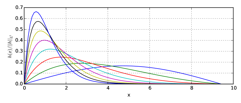
Figure 3. Shape of the normalized principal eigenfunction $H_{1}$, which corresponds to the average profile of the normalized order book, for $L:=3\pi$, $\eta:=1$ and different values of $\beta\in\{0,0.5,...3.5\}$.

The above results are valuable for calibrating the model parameters $\frac{\beta}{2\eta}$, $\alpha$ and $\sigma$ to reproduce the average profile (for each side) of the order book.

$\frac{\beta}{2\eta}$ can be estimated from the position $\hat{x}$ of the maximum using (3.24). Note that, when $L$ is large then

$$\hat{x}\approx\frac{2\eta}{\beta}.$$

The height of this maximum gives a further constraint on parameters, using (3.25).

We will use this result for parameter estimation in Section 3.6.

3.3. Dynamics of order book volume

As noted in Corollary 3.3, $V^{a}_{t}$ and $V^{b}_{t}$ may be identified as the volume of sell (resp. buy) limit orders: they follow (correlated) geometric Brownian motions:

$$V_{t}^{a} =\int_{0}^{L}\left\lvert u_{t}(x)\right\rvert\,\operatorname{d}x=V^{a}_{0}\exp(\sigma_{a}W^{a}_{t}-\nu_{a}t-\frac{\sigma_{a}^{2}t}{2})$$

$$V_{t}^{b} =\int_{-L}^{0}\left\lvert u_{t}(x)\right\rvert\,\operatorname{d}x=V^{b}_{0}\exp(\sigma_{b}W^{b}_{t}-\nu_{b}t-\frac{\sigma_{b}^{2}t}{2})$$

where $[W^{a},W^{b}]_{t}=\rho_{a,b}t$. The average volume of the order book $V_{t}=V^{a}_{t}+V^{b}_{t}$ satisfies

$$\mathbb{E}(V_{t})=V_{0}-\int_{0}^{t}V^{0}_{a}\nu_{a}e^{-\nu_{a}s}-V^{0}_{b}\nu_{b}e^{-\nu_{b}s}\,\operatorname{d}s=V_{0}+V^{0}_{a}e^{-\nu_{a}t}+V^{0}_{b}e^{-\nu_{b}t}.$$

Intraday studies of order book volume show it to be stable away from the open and close. Here $\mathbb{E}V_{t}=V_{a}+V_{b}$ if and only if $V$ is a martingale, i. e. $\nu_{a}=\nu_{b}=0$.

3.4. Dynamics of price and market depth

Recall from the discussion in Section 1.3 that the order book dynamics yield the price process

$$\,\operatorname{d}S_{t}=\theta\left(\frac{\,\operatorname{d}D_{t}^{b}}{D_{t}^{b}}-\frac{\,\operatorname{d}D_{t}^{a}}{D_{t}^{a}}\right),$$

where $\theta$ is an impact coefficient and $D_{t}^{b}$ and $D_{t}^{a}$ represent the depth at the top of the order book [Cont et al., 2014]:

(3.26) $$D_{t}^{a}:=\int_{0}^{\delta}u_{t}(x)\,\operatorname{d}x\approx\frac{1}{2}\delta^{2}\nabla u_{t}(0+),\quad D_{t}^{b}:=\int_{-\delta}^{0}|u_{t}(x)|\,\operatorname{d}x\approx\frac{1}{2}\delta^{2}\nabla u_{t}(0-).$$

Using the results in Corollary 3.3, we obtain the following price dynamics:

(3.27) $$\,\operatorname{d}S_{t}=\theta\left(\frac{\,\operatorname{d}V_{t}^{b}}{V_{t}^{b}}-\frac{\,\operatorname{d}V_{t}^{a}}{V_{t}^{a}}\right),$$

where

(3.28) $$\,\operatorname{d}V_{t}^{b}=-\nu_{b}V_{t}^{b}\,\operatorname{d}t+\sigma_{b}V_{t}^{b}\,\operatorname{d}W_{t}^{b},\quad\,\operatorname{d}V_{t}^{a}=-\nu_{a}V_{t}^{a}\,\operatorname{d}t+\sigma_{a}V_{t}^{a}\,\operatorname{d}W_{t}^{a}.$$

The price dynamics can thus be written as

$$S_{t} =S_{0}-\theta t\left(\nu_{b}-\nu_{a}\right)+\theta\sigma_{b}W_{t}^{b}-\theta\sigma_{a}W_{t}^{a}$$

$${=}S_{0}-\theta t\left(\nu_{b}-\nu_{a}\right)+\sigma_{S}B_{t}$$

where $B$ is a Brownian motion and $\sigma_{S}$ is the mid price volatility, which may be expressed in terms of parameters describing the order flow:

(3.29) $$\sigma_{S}:=\theta\sqrt{\sigma_{b}^{2}+\sigma_{a}^{2}-2\sigma_{a}\sigma_{b}\varrho_{a,b}}.$$

The implied price dynamics thus corresponds to the Bachelier model:

• The drift term $\nu_{a}-\nu_{b}$ only depends on the rate of relative increase of the bid/ask depth, not the actual depths $D^{b}_{t}$ and $D^{a}_{t}$.

• The quadratic variation of the mid price is $\sigma_{S}^{2}t$ decreases with the correlation between the buy and sell order flow. This correlation, generated by market makers, reduces price volatility.

Remark 3.6.

Replacing $\sigma_{a}W^{a}$ and $\sigma_{b}W^{b}$ by arbitrary semimartingales $X^{a}$ and $X^{b}$ with jumps bounded from below by $-1$, yields the following price dynamics:

(3.30) $$S_{t}=S_{0}-\theta t\left(\nu_{b}-\nu_{a}\right)+\theta(X_{t}^{b}-X_{t}^{a}).$$

In particular, this relation links price jumps to large changes (‘jumps’) in order flow imbalance:

(3.31) $$\Delta S_{t}=\theta\ \Delta(X_{t}^{b}-X_{t}^{a}).$$

3.5. Absolute price coordinates: stochastic moving boundary problem

The model above describes dynamics of the order book in relative price coordinates, i.e. as a function of the (scaled) distance $x$ from the mid-price. The density of the limit order book parameterized by the (absolute) price level $p\in\mathbb{R}$ is given (in the case of linear scaling) by

(3.32) $$v_{t}(p)=u_{t}(p-S_{t}),\qquad x\in\mathbb{R},$$

where we extend $u_{t}$ to $\mathbb{R}$ by setting $u_{t}(y)=0$ for $y\in\mathbb{R}\setminus[-L,L]$. As observed in Section 3.4, the mid-price dynamics is given by

(3.33) $$\,\operatorname{d}S_{t}=-\theta(\nu_{b}-\nu_{a})\,\operatorname{d}t+\theta\sigma_{b}\,\operatorname{d}W_{t}^{b}-\theta\sigma_{a}\,\operatorname{d}W_{t}^{a}.$$

The dynamics of $v$ may then be described, via an application of the Itô-Wentzell formula, as the solution of a stochastic moving boundary problem [Mueller, 2018]:

Theorem 3.7 (Stochastic moving boundary problem).

The order book density $v_{t}(p)$, as a function of the price level $p$ is a solution, in the sense of distributions, of the stochastic moving boundary problem

(3.34) $$\,\operatorname{d}v_{t}(p)=\left[(\eta_{a}+\tfrac{1}{2}\sigma_{s}^{2})\Delta v_{t}(p)\right.\\ \left.+(\nu_{b}-\nu_{a}+\beta_{a}-\theta(\varrho_{a,b}\sigma_{b}\sigma_{a}-\sigma_{a}^{2})\nabla v_{t}(p)+\alpha_{a}v_{t}(p)\right]\,\operatorname{d}t\\ +\left(\sigma_{a}v_{t}(p)+\theta\sigma_{a}\nabla v_{t}(p)\right)\,\operatorname{d}W_{t}^{a}-\theta\sigma_{b}\nabla v_{t}(p)\,\operatorname{d}W_{t}^{b},$$

for $p\in(S_{t},S_{t}+L)$, and

(3.35) $$\,\operatorname{d}v_{t}(p)=\left[(\eta_{b}+\tfrac{1}{2}\sigma_{s}^{2})\Delta v_{t}(p)\right.\\ \left.+(\nu_{b}-\nu_{a}-\beta_{b}-\theta(\sigma_{b}^{2}-\varrho_{a,b}\sigma_{b}\sigma_{a}))\nabla v_{t}(x)+\alpha_{b}v_{t}(p)\right]\,\operatorname{d}t\\ +\theta\sigma_{a}\nabla v_{t}(p)\,\operatorname{d}W_{t}^{a}+\left(\sigma_{b}v_{t}(p)-\theta\sigma_{b}\nabla v_{t}(p)\right)\,\operatorname{d}W_{t}^{b}$$

for $x\in(S_{t}-L,S_{t})$ with the moving boundary conditions

(3.36) $$v_{t}(S_{t})=0,\qquad v_{t}(y)=0,\qquad\forall y\in\mathbb{R}\setminus(S_{t}-L,S_{t}+L),$$

in the following sense: $(v_{t})_{t\geq 0}$ is an continuous $L^{2}(\mathbb{R})$-valued stochastic process and for all $\varphi\in C^{\infty}_{0}(\mathbb{R})$ and $t\geq 0$,

(3.37) $$\langle v_{t},\varphi\rangle-\langle v_{0},\varphi\rangle=\int_{0}^{t}\langle m(x-S_{t},\Delta v_{r},\nabla v_{r},v_{r}),\varphi\rangle\,\operatorname{d}r\quad+\\ \frac{1}{2}\int_{0}^{t}\left(\nabla v_{r}(S_{r}-)-\nabla v_{r}(S_{r}+))\varphi(S_{r})-\nabla v_{r}(S_{r}-L+)\varphi(S_{r}-L)+\nabla v_{r}(S_{r}+L-)\varphi(S_{r}+L)\right)d\langle S\rangle_{r}\\ +\int_{0}^{t}\langle\mathbf{1}_{(S,S_{r}+L)}\sigma_{a}v_{r},\varphi\rangle\,\operatorname{d}W_{r}^{a}+\int_{0}^{t}\langle\mathbf{1}_{(S_{r}-L,S_{r})}\sigma_{b}v_{r},\varphi\rangle\,\operatorname{d}W^{b}_{r}\\ +\theta\sigma_{a}\int_{0}^{t}\langle\nabla v_{r},\varphi\rangle\,\operatorname{d}W^{a}_{r}-\theta\sigma_{b}\int_{0}^{t}\langle\nabla v_{r},\varphi\rangle\,\operatorname{d}W^{b}_{r},$$

where we denote, for $S\in\mathbb{R}$, $V\in H^{1}_{0}((-L,L)\setminus\{0\})\cap H^{2}((-L,L)\setminus\{0\})$,

$$m(x,y^{\prime\prime},y^{\prime},y)=\begin{cases}(\eta_{a}+\tfrac{1}{2}\sigma_{s}^{2})y^{\prime\prime}&\\ +(\nu_{b}-\nu_{a}+\beta_{a}-\theta(\varrho_{a,b}\sigma_{b}\sigma_{a}-\sigma_{a}^{2}))y^{\prime}+\alpha_{a}y,&x\in(0,L),\\ (\eta_{b}+\theta\sigma_{s}^{2})y^{\prime\prime}&\\ +(\nu_{b}-\nu_{a}-\beta_{b}-\theta(\sigma_{b}^{2}-\varrho_{a,b}\sigma_{b}\sigma_{a})))y^{\prime}+\alpha_{b}y,&x\in(-L,0)\\ 0,&\text{ else,}\end{cases}$$

for $x,y^{\prime\prime},y^{\prime},y\in\mathbb{R}$.

Remark 3.8.

Note that (3.36) is a stochastic boundary condition at $S_{t}$.

The proof, given in Appendix A, is based on Krylov’s extended Itô-Wentzell formula [Krylov, 2011, Theorem 1.1].

3.6. Parameter estimation

We now describe a method for estimating model parameters. We use time series of order books for NASDAQ stocks and ETFs, from the LOBSTER database.

Given that we do not observe separately the various components of the order flow as in (3.1), we use the relations discussed in Sec. 3.2 to calibrate the parameters $\sigma$, $\nu$ and the shape parameter

(3.38) $$\gamma:=\frac{\beta}{2\eta}.$$

for each side of the order book. We set $L$ to the largest value in our data set, ($L:=1000$). Parameters may be calibrated either through

1. a least squares fit of (3.23) to the average order book profile, or

2. calibrating parameters to reproduce the position $\hat{x}$ and height of the maximum of the order book profile.

Remark 3.9.

The estimator based on the maximum position of the peak is fast in computation but the fixed price level grid in the data restricts the set possible values for estimation of $\gamma$. In particular, the estimator is sensitive to the location of the maximum (i.e. the mode of the order book profile).

We show results for a set of NASDAQ stocks and ETFs. Figure 4 shows how the model reproduces the average book profile for QQQ at NASDAQ on 17th November 2017. In Figure 5 we see the coefficient $\gamma$ estimated across various 30-min windows during the trading day. The one-factor model based on the principal eigenfunction yields a reasonable approximation for the average order book profile, which justifies our assumptions on the dynamics in Section 1.2.

For low-price/large tick stocks, the average order book profiles may differ from the exponential-sine shape. For such stocks, we use the nonlinear scaling described in Section 1.1, leading to an average order book profile:

(3.39) $$U(p)=V\exp(-\gamma((p-S_{t})/\delta)^{a})\sin\left(((p-S_{t})/\delta)^{a}\pi/L\right)),$$

where $S_{t}$ is the best price. Figure 6 shows such a nonlinear fit for the average order book profile of SIRI.

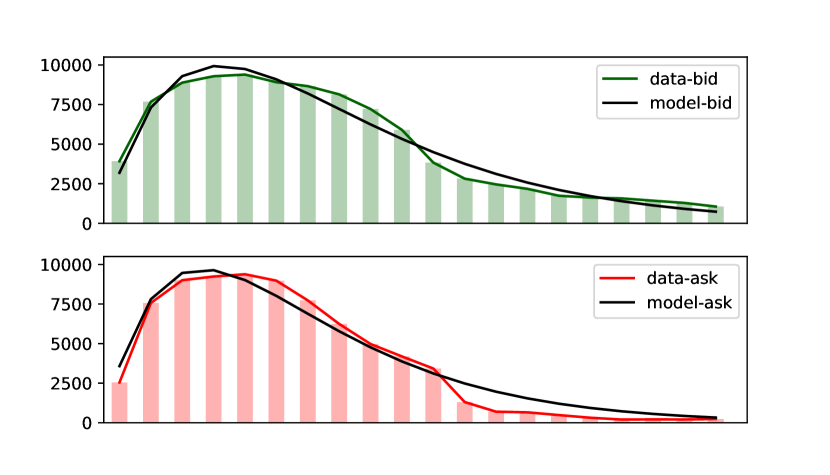
Figure 4. Average profile of QQQ order book (first 20 levels), 17 Nov 2016 (Top: bid, Bottom: ask).

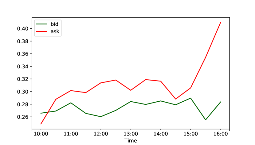
Figure 5. Values of parameter $\gamma_{a},\gamma_{b}$ estimated from 30 min average profile of QQQ order book (first 20 levels), 17 Nov 2016.

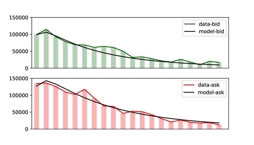
Figure 6. Average profile of SIRI order book (first 20 levels, 17th November 2016)(Top: bid, Bottom: ask) $\gamma_{b}=0.95$, $\gamma_{a}=0.86$, $a_{b}=0.52$, $a_{a}=0.56$.

4. Mean-reverting models

4.1. A class of models with mean-reversion

We now return to the full model (1.2) with non-zero source terms $f^{a}(x),f^{b}(x)$ representing the rate of arrival of new limit orders at a distance $x$ from the best price:

$$\begin{split}\,\operatorname{d}u_{t}(x)&=\left[\eta_{a}\Delta u_{t}(x)+\beta_{a}\nabla u_{t}(x)+\alpha_{a}u_{t}(x)+f^{a}(x)\right]\,\operatorname{d}t+\sigma_{a}u_{t}(x)\,\operatorname{d}W^{a}_{t},\quad\,x\in(0,L),\\ \,\operatorname{d}u_{t}(x)&=\left[\eta_{b}\Delta u_{t}(x)-\beta_{b}\nabla u_{t}(x)+\alpha_{b}u_{t}(x)+f^{b}(x)\right]\,\operatorname{d}t+\sigma_{b}u_{t}(x)\,\operatorname{d}W^{b}_{t},\quad\,x\in(-L,0),\\ u_{t}(0+)&=u_{t}(0-)=0,\qquad u_{t}(-L)=u_{t}(L)=0,\quad t>0,\end{split}$$

with the sign condition

$$u_{t}(x)\leq 0,\quad x\in(-L,0),\quad\text{and}\quad u_{t}(x)\geq 0,\quad x\in(0,L),\;t\geq 0,$$

where, as above $\eta_{a}$, $\eta_{b}$, $\sigma_{a}$, $\sigma_{b}>0$, $\beta_{a}$, $\beta_{b}\geq 0$, $\alpha_{a}$, $\alpha_{b}\in\mathbb{R}$ are constants and $u_{0}\in L^{2}((-L,L))$. As above, we denote $u^{b}_{0}:=u_{0}|_{[-L,0]}$ and $u^{a}_{0}:=u_{0}|_{[0,L]}$. We will show that, when $\alpha_{a}$ and $\alpha_{b}$ are negative and $f^{a}(x)>0$, $f^{b}(-x)<0$ for all $x\in(0,L)$, this class of models leads to mean reverting dynamics for the order book profile, consistent with the observation that intraday dynamics of order book volume and queue size over intermediate time scales (hours, day) typically exhibit mean reversion rather than a trend.

Projecting the equation on the eigenfunctions $h_{k}^{a},h_{k}^{b}$, as in Section 3, we see that, due to the fast increase in the eigenvalues (3.4), solutions starting from a generic initial condition may be approximated by their projection on the principal eigenfunctions $h_{1}^{a},h_{1}^{b}$ (we will justify this below in Proposition 4.2) and the main contribution of heterogeneous order arrivals arises from the projection of $f^{a}$ (resp. $f^{b}$) on $h_{1}^{a}$ (resp. $h_{1}^{b}$).

This motivates the following specfication, which leads to a tractable class of models:

(4.1) $$f^{a}(x):=\bar{V}_{a}\ H_{1}^{a}(x),\qquad f^{b}(x):=\bar{V}_{b}\ H_{1}^{b}(x),\quad\bar{V}_{a}>0,\quad\bar{V}_{b}>0$$

Theorem 2.10 then gives explicit solutions to (1.2). Recall the notations (3.10) and (3.9) and define $V_{t}^{b}$ and $V_{t}^{a}$ by

(4.2) $$\,\operatorname{d}V_{t}^{a}=\left(\bar{V}_{a}-\nu_{a}V_{t}^{a}\right)\,\operatorname{d}t+\sigma_{a}V_{t}^{a}\,\operatorname{d}W_{t}^{a}, \,\operatorname{d}V_{t}^{b}=\left(\bar{V}_{b}-\nu_{b}V_{t}^{b}\right)\,\operatorname{d}t+\sigma_{b}V_{t}^{b}\,\operatorname{d}W_{t}^{b}$$

where $\nu_{i}:=\frac{\eta_{i}\pi^{2}}{L^{2}}+\frac{\beta_{i}^{2}}{4\eta_{i}}-\alpha_{i}$, $i\in\{a,\,b\}$. The solution of the SPDE may then be obtained as follows:

Proposition 4.1.

1. The unique $L^{2}$-continuous solution of (1.2) – (4.1) for a general initial condition $u_{0}$ is given by

   $$u_{t}(x)=\begin{cases}V_{t}^{b}H_{1}^{b}(x)+\mathcal{E}_{t}(\sigma_{b}W^{b})\sum_{k=1}^{\infty}e^{-\nu_{k}^{b}t}\left\langle u_{0}^{b}-V_{0}^{b}H_{1}^{b},h_{k}^{b}\right\rangle_{(-\frac{\beta_{b}}{2\eta_{b}})}h_{k}^{b}(x),&x\in(-L,0),\\ V_{t}^{a}H_{1}^{a}(x)+\mathcal{E}_{t}(\sigma_{a}W^{a})\sum_{k=1}^{\infty}e^{-\nu_{k}^{a}t}\left\langle u_{0}^{a}-V_{0}^{a}H_{1}^{a},h_{k}^{a}\right\rangle_{\frac{\beta_{a}}{2\eta_{a}}}h_{k}^{a}(x),&x\in(0,L),\\ 0,\qquad x\notin(-L,0)\cup(0,L).&\end{cases}$$

2. For an initial condition of the form

   $$u_{0}(x)=V_{0}^{a}H_{1}^{a}(x)\mathbf{1}_{[0,L]}+V_{0}^{b}H_{1}^{b}(x)\mathbf{1}_{[-L,0]}$$

   the unique $L^{2}$-continuous solution of (1.2) – (4.1) is given by

   (4.3) $$u_{t}(x)=\left(V_{t}^{a}H_{1}^{a}(x)\mathbf{1}_{(0,L)}(x)+V_{t}^{b}H_{1}^{b}(x)\mathbf{1}_{(-L,0)}(x)\right),\quad x\in[-L,L].$$

Proof.

We obtain the general solution of the linear homogeneous equation from Proposition 3.2. The series representation of $u$ results from the spectral decomposition, Proposition 3.1 and Theorem 2.10. ∎

4.2. Long time asymptotics and stationary solutions

In order to derive properties of the ’average’ order book profile, we now examine whether the order book profile $u_{t}$ has an ergodic behavior and describe stationary solutions. The following result describes the long-term dynamics and shows that this dynamics is well approximated by projecting the initial condition on the principal eigenfunctions as done in (4.3):

Proposition 4.2.

Let $u_{t}$ be the unique solution of (1.2) – (4.1) for a general initial condition $u_{0}\in L^{2}(-L,L)$ and define:

(4.4) $$\check{u}_{t}(x):=V^{b}_{t}H^{b}_{1}(x)\mathbf{1}_{(-L,0)}(x)+V^{a}_{t}H^{a}_{1}(x)\mathbf{1}_{(0,L)}(x),\qquad t>0.$$

If $\nu_{1}^{b}>0$ and $\nu_{1}^{a}>0$, then:

1. The long-term dynamics of the order book is well approximated by the dynamics (4.4) projected along the principal eigenfunctions:

   (4.5) $$\mathbb{P}\left(\lim_{t\to\infty}\left\lVert u_{t}-\check{u}_{t}\right\rVert_{\infty}=0\quad\right)=1.$$

2. $u_{t}$ has a unique stationary distribution and

   (4.6) $$u_{t}(x)\underset{t\to\infty}{\Longrightarrow}f^{b}(x)Z^{b},\quad x<0,\qquad u_{t}(x)\underset{t\to\infty}{\Longrightarrow}f^{a}(x)Z^{a},\quad x>0,$$

   where $f^{a},f^{b}$ are given by (4.1) and $Z^{a}$ (resp. $Z^{b}$ ) is an Inverse Gamma random variable with shape parameter $1+2\frac{\nu_{a}}{\sigma_{a}^{2}}$ (resp. $1+2\frac{\nu_{b}}{\sigma_{b}^{2}}$) and scale parameter $\frac{\sigma_{a}^{2}}{2\bar{V}_{a}}$ (resp. $\frac{\sigma_{b}^{2}}{2\bar{V}_{b}}$).

3. If furthermore $\nu_{1}^{b}>\frac{\sigma_{b}^{2}}{2}$ and $\nu_{1}^{a}>\frac{\sigma^{2}_{a}}{2}$, then

   (4.7) $$\lim_{t\to\infty}\mathbb{E}\left[\left\lVert u_{t}-\check{u}_{t}\right\rVert_{L^{2}(-L,L)}^{2}\right]=0.$$

Proof.

For $t_{0}>0$, let

$$K_{t_{0}}:=\sqrt{\sum_{k=1}^{\infty}e^{-2(\nu_{k}^{a}-\nu_{1}^{a})t_{0}}}<\infty.$$

This term is indeed finite by integral criterion for series, see e. g. proof of Proposition 3.2. Denote $u_{t}^{\circ}(.;h)$ the unique solution of the linear homogeneous equation (3.1) for an initial condition $h$. Recall from Theorem 2.10 that

$$u_{t}(x)-\check{u}_{t}(x)=u_{t}^{\circ}(x;u_{0}-\check{u}_{0}).$$

It suffices now to prove the results for the ask side and note that the calculations will be analogous for the bid side. Using the representation of $u_{t}^{\circ}$ from Proposition 3.2 we get for all $t>t_{0}$ and all $h\in L^{2}(0,L)$,

$$\left\lVert u_{t}^{\circ}(.;h)|_{(0,L)}\right\rVert_{\infty} \leq e^{-\nu_{1}^{a}t}\mathcal{E}_{t}(\sigma_{a}W^{a})\sqrt{\sum_{k=1}^{\infty}e^{-2(\nu_{k}^{a}-\nu_{1}^{a})t_{0}}}\sqrt{\sum_{k=1}^{\infty}\left\lvert\left\langle h,h^{a}_{k}\right\rangle_{\frac{\beta_{a}}{2\eta_{a}}}\right\rvert^{2}}$$

$$=K_{t_{0}}\left\lVert h\right\rVert_{\frac{\beta_{a}}{2\eta_{a}}}\exp\left(\sigma_{a}W^{a}_{t}-\left(\nu_{1}^{a}+\tfrac{\sigma_{a}^{2}}{2}\right)t\right),$$

which, as $t\to\infty$, converges to $0$ provided that $\nu_{1}^{a}>0$. This proves (i).

To show (iii), a similar calculation but using the orthogonality of the decomposition in Proposition 3.2 yields

$$\mathbb{E}\left[\left\lVert u_{t}^{\circ}(.;h)|_{(0,L)}\right\rVert_{\frac{\beta_{a}}{2\eta_{a}}}^{2}\right] =\sum_{k=1}^{\infty}e^{-2\nu_{k}^{a}t}\left\lvert\left\langle h,h^{a}_{k}\right\rangle_{\frac{\beta_{a}}{2\eta_{a}}}\right\rvert^{2}\mathbb{E}\left[\left\lvert\mathcal{E}_{t}(\sigma_{a}W^{a})\right\rvert^{2}\right]$$

$$\leq e^{-2\nu_{1}^{a}t}\left\lVert h\right\rVert_{\frac{\beta_{a}}{2\eta_{a}}}^{2}\mathbb{E}\left[\exp\left(2\sigma_{a}W^{a}_{t}-\sigma_{a}^{2}t\right)\right]$$

$$=e^{(-2\nu^{a}_{1}+\sigma^{2}_{a})t}\left\lVert h\right\rVert_{\frac{\beta_{a}}{2\eta_{a}}}^{2}.$$

If $\sigma_{a}^{2}<2\nu_{1}^{a}$, then this converges to $0$ as $t\to\infty$. Since $\left\lVert.\right\rVert_{\frac{\beta_{a}}{2\eta_{a}}}$ defines an equivalent norm on $L^{2}(0,L)$, this finishes the proof of (iii).

Assertion (ii) follows from Proposition 2.13. Indeed, recall that $V^{i},i\in\{a,b\}$ are ergodic processes whose unique invariant distribution is given by an Inverse Gamma distribution with shape parameter $1+\frac{2\nu_{i}}{\sigma_{i}^{2}}$ and scale parameters $\frac{\sigma_{i}^{2}}{(\bar{V}_{i})^{2}}$, $i\in\{a,\,b\}$. Denote by $Z^{b}$ and $Z^{a}$ random variables with these distribution For any $x\in[-L,L]$, we have the convergence in distribution

(4.8) $$\check{u}_{t}|_{(-L,0)}\Longrightarrow Z^{b}\ f^{b}_{1}(.),\qquad\check{u}_{t}|_{(0,L)}\Longrightarrow Z^{a}\ f^{a}(.).$$

Since almost sure convergence yields convergence in distribution, by part (i) this yields that (4.8) holds also for $u_{t}$ with arbitrary initial data $u_{0}\in L^{2}(-L,L)$. ∎

4.3. Dynamics of order book volume

Consider now the ‘projected’ dynamics as in the setting of Proposition 4.1.(ii). The dynamics of the order book volume $V_{t}$ is then given by

(4.9) $$V_{t}:=\int_{-L}^{L}\left\lvert u_{t}(x)\right\rvert\,\operatorname{d}x=V^{b}_{t}+V_{t}^{a},\qquad t\geq 0,$$

where $V^{b}$ and $V^{a}$, defined in (4.2), represent the volume of buy (resp. sell) orders in the order book.

Since $[W^{a},W^{b}]_{t}=\varrho_{a,b}t$ we can write

$$W^{a}=:W,\qquad W^{b}:=\varrho_{a,b}W+\sqrt{1-\varrho_{a,b}^{2}}\widehat{W},$$

for some Brownian motion $\widehat{W}$, independent of $W$. Then,

(4.10) $$\,\operatorname{d}V_{t}=(\bar{V}_{a}+\bar{V}_{b}-(\nu_{a}V_{t}^{a}+\nu_{b}V_{t}^{b})\,\operatorname{d}t\\ +\left(\sigma_{a}V_{t}^{a}+\varrho_{a,b}\sigma_{b}V_{t}^{b}\right)\,\operatorname{d}W_{t}+\sqrt{1-\varrho_{a,b}^{2}}\sigma_{b}V_{t}^{b}\,\operatorname{d}\widehat{W}_{t}.$$

In particular, the quadratic variation (‘realized variance’) of the order book volume is given by

(4.11) $$\,\operatorname{d}\langle V\rangle_{t}=\left(\sigma_{a}^{2}(V_{t}^{a})^{2}+2\varrho_{a,b}\sigma_{b}\sigma_{a}V_{t}^{a}V_{t}^{b}+\sigma_{b}^{2}(V_{t}^{b})^{2}\right)\,\operatorname{d}t$$

For the symmetric and perfectly correlated case, $V$ is itself a reciprocal gamma diffusion:

Corollary 4.3.

Assume the setting of Proposition 4.1.(ii) and, in addition, that $\nu_{a}=\nu_{b}=:\nu$, $\sigma_{a}=\sigma_{b}=:\sigma$ and $\varrho_{a,b}=1$. Then, $V$ is the unique solution of

(4.12) $$\,\operatorname{d}V_{t}=\left((\bar{V}_{b}+\bar{V}_{a})-\nu V_{t}\right)\,\operatorname{d}t+\sigma V_{t}\,\operatorname{d}W_{t},$$

with $V_{0}=V_{0}^{b}+V_{0}^{a}$.

In all cases, we get from (2.22) that for $i\in\{a,b\}$, $t\geq 0$,

(4.13) $$\mathbb{E}V_{t}^{i}=\left(V_{0}^{i}-\frac{\nu_{i}}{\bar{V}_{i}}\right)e^{-\nu_{i}t}+\frac{\nu_{i}}{\bar{V}_{i}}$$

and

(4.14) $$\mathbb{E}V_{t}^{i}=\left(V_{0}^{b}-\frac{\bar{V}_{b}}{\nu_{b}}\right)e^{-\nu_{b}t}+\left(V_{0}^{a}-\frac{\bar{V}_{a}}{\nu_{a}}\right)e^{-\nu_{a}t}+\frac{\bar{V}_{b}}{\nu_{b}}+\frac{\bar{V}_{a}}{\nu_{a}}.$$

4.4. Joint dynamics of mid-price and market depth

We now consider the mid price and market depths dynamics in the situation of Proposition 4.1.(ii). As discussed in Sections 1.3 and Section 3.4 for the linear homogeneous models, the dynamics of the mid-price is given by

$$\,\operatorname{d}S_{t}=\theta\left(\frac{\,\operatorname{d}D_{t}^{b}}{D_{t}^{b}}-\frac{\,\operatorname{d}D_{t}^{a}}{D_{t}^{a}}\right),$$

where $\theta$ is an impact coefficient, while the bid/ask depths follow

$$D_{t}^{a} :=\int_{0}^{\delta}u_{t}(x)\,\operatorname{d}x\approx\frac{1}{2}\delta^{2}\nabla u_{t}(0+)=\frac{\pi}{2L}\delta^{2}V_{t}^{a},$$

$$D_{t}^{b} :=-\int_{-\delta}^{0}u_{t}(x)\,\operatorname{d}x\approx\frac{1}{2}\delta^{2}\nabla u_{t}(0-)=\frac{\pi}{2L}\delta^{2}V_{t}^{a}.$$

Thus, the dynamics of the market depths are given by

$$\,\operatorname{d}D_{t}^{b} =\nu_{b}\left(\overline{D}_{b}-D_{t}^{b}\right)\,\operatorname{d}t+\sigma_{b}D_{t}^{b}\,\operatorname{d}W_{t}^{b},$$

$$\,\operatorname{d}D_{t}^{a} =\nu_{a}\left(\overline{D}_{a}-D_{t}^{a}\right)\,\operatorname{d}t+\sigma_{a}D_{t}^{a}\,\operatorname{d}W_{t}^{a}.$$

for some mean reversion levels $\overline{D}_{b},\overline{D}_{a}>0$. We thus obtain the joint dynamics of price and market depth:

(4.15) $$\,\operatorname{d}\begin{pmatrix}D_{t}^{b}\\ D_{t}^{a}\\ S_{t}\end{pmatrix}=\begin{pmatrix}\nu_{b}(\overline{D}_{b}-D_{t}^{b})\\ \nu_{a}(\overline{D}_{a}-D_{t}^{a})\\ \theta\left(\frac{\nu_{b}\overline{D}_{b}}{D_{t}^{b}}-\frac{\nu_{a}\overline{D}_{a}}{D_{t}^{a}}-(\nu_{b}-\nu_{a})\right)\end{pmatrix}\,\operatorname{d}t\\ +\begin{pmatrix}\sigma_{b}D_{t}^{b}&0\\ \varrho_{a,b}\sigma_{a}D_{t}^{a}&\sqrt{1-\varrho_{a,b}^{2}}\sigma_{a}D_{t}^{a}\\ \theta\left(\sigma_{b}-\varrho_{a,b}\sigma_{a}\right)&-\theta\sqrt{1-\varrho_{a,b}^{2}}\sigma_{a}\end{pmatrix}\,\operatorname{d}\begin{pmatrix}W^{1}_{t}\\ W_{t}^{2}\end{pmatrix},$$

where $W^{1}$ and $W^{2}$ are independent Brownian motions. The mid-price itself has quadratic variation $\langle S\rangle_{t}=\sigma_{S}^{2}t$, where

(4.16) $$\sigma_{S}:=\theta\sqrt{\sigma_{b}^{2}+\sigma_{a}^{2}-2\sigma_{a}\sigma_{b}\varrho_{a,b}}.$$

Over a small time interval $\Delta t,$

$$S_{\Delta t} =S_{0}+\theta\int_{0}^{\Delta t}\frac{\nu_{b}(\overline{D}_{b}-D^{b}_{s})}{D^{b}_{s}}-\frac{\nu_{a}(\overline{D}_{a}-D^{a}_{s})}{2D^{a}(s)}\,\operatorname{d}s+\theta\sigma_{b}W_{\Delta t}^{b}-\theta\sigma_{a}W_{\Delta t}^{a}$$

$$\approx S_{0}+{\Delta t}\frac{\theta}{2}\left(\frac{\nu_{b}(\overline{D}_{b}-D_{0}^{b})}{D_{0}^{b}}-\frac{\nu_{a}(\overline{D}_{a}-D_{0}^{a})}{D_{0}^{a}}\right)+\sigma_{S}\sqrt{\Delta t}\ N_{0,1}$$

where $N_{0,1}$ is a standard Gaussian variable. In particular the conditional probability of an upward mid-price move of size $y$ is given by

(4.17) $$\mathbb{P}\left[S_{\Delta t}\geq S_{0}+y\right]\simeq N\left(\frac{\theta\sqrt{{\Delta t}}}{\sigma_{S}}\left(\frac{\nu_{b}(\overline{D}_{b}-D_{0}^{b})}{D^{b}_{0}}-\frac{\nu_{a}(\overline{D}_{a}-D_{0}^{a})}{D^{a}_{0}}\right)-\frac{y}{\sigma_{S}\sqrt{{\Delta t}}}\right),$$

where $N$ denotes the cumulative distribution function of the standard normal distribution.

Remark 4.4.

Using (2.22), the expected order flow over a small time interval $[0,t]$ on each side of the book is given by for $\star\in\{a,b\}$,

(4.18) $$\mathbb{E}\left[D_{t}^{\star}-D_{0}^{\star}\right]=t\nu_{\star}(\overline{D}_{\star}-D_{0}^{\star})+o(t).$$

Remark 4.5 (Mean-reverting order book imbalance).

The imbalance between buy and sell depth is a frequently used indicator for predicting short term price moves [Cartea et al., 2018, Cont and de Larrard, 2013, Lipton et al., 2014]). In this model, the depth imbalance has the following dynamics:

$$\,\operatorname{d}(D^{b}_{t}-D^{a}_{t})=\left(\nu^{b}\overline{D}^{b}-\nu^{a}\overline{D}^{a}-(\nu^{b}D^{b}_{t}-\nu^{a}D^{a}_{t})\right)\,\operatorname{d}t+\sigma_{b}D^{b}_{t}\,\operatorname{d}W^{b}_{t}-\sigma_{a}D_{t}^{a}\,\operatorname{d}W_{t}^{a}.$$

In the symmetric case, when $\overline{D}=\overline{D}_{a}=\overline{D}_{b}$, $\nu=\nu_{a}=\nu_{b}$, (4.17) becomes

(4.19) $$N\left(\frac{\nu\overline{D}\theta\sqrt{t}}{\sigma_{S}}\frac{\left(D^{a}_{0}-D^{b}_{0}\right)}{D^{a}_{0}D^{b}_{0}}-\frac{y}{\sigma_{S}\sqrt{t}}\right).$$

This quantity is decreasing in the depth imbalance $D^{b}_{0}-D^{a}_{0}$: this is a consequence of the mean reversion in order book depth. In the symmetric case

(4.20) $$\,\operatorname{d}(D^{b}_{t}-D^{a}_{t})=-\nu\left(D^{b}_{t}-D^{a}_{t})\right)\,\operatorname{d}t+\sigma_{b}D^{b}_{t}\,\operatorname{d}W^{b}_{t}-\sigma_{a}D_{t}^{a}\,\operatorname{d}W_{t}^{a},$$

so the model reproduces the empirical observation that order book imbalance is mean reverting [Cartea et al., 2018].

Note that the model predicts mean reversion of market depths on the scale of $1/\nu$ which corresponds to seconds for the ETFs QQQ and SPY and around 10 seconds for large tick stocks such as MSFT and INTC (see Table 1). For time scales smaller than $1/\nu$, the direction of price moves is highly correlated with order flow imbalance, as shown in empirical studies of equity markets [Cont et al., 2014].

4.5. Parameter estimation

We now discuss estimation of model parameters from a discrete set of observations $(V^{a}_{n},V^{b}_{n})_{n=0,\ldots,N}$ of the bid/ask volumes $V^{a}_{t},V^{b}_{t}$ on a uniform time grid $\{k\Delta t\,\colon\,k=0,\ldots,N\}$. Let us rewrite the dynamics of $V^{a}_{t}$ and $V^{b}_{t}$ in the form of reciprocal Gamma diffusions:

(4.21) $$\,\operatorname{d}V^{\star}_{t}=\nu_{\star}\left(\overline{D}_{\star}-V_{0}^{\star}\right)+\sqrt{2\frac{\nu_{\star}}{c_{\star}}(V_{t}^{\star})^{2}}\,\operatorname{d}W^{\star}_{t},\quad t\geq 0,\quad V_{0}^{\star}\in(0,\infty),\star\in\{a,b\}$$

with $\nu_{\star}$, $\overline{D}_{\star}$, $c_{\star}>0$. We use method of moments estimators as in [Leonenko and Šuvak, 2010] for $\overline{D}_{\star}$ and $c_{\star}$ and a martingale estimation function [Bibby and Sørensen, 1995] for the autocorrelation parameters $\nu_{\star}$, $\star\in\{a,b\}$: we define

$$\widehat{\overline{D}_{\star}}:=\frac{1}{N}\sum_{k=1}^{N}\hat{V}_{k},\quad{\rm and}\quad\hat{c_{\star}}:=\frac{\sum_{n=1}^{N}(\hat{V}_{n})^{2}}{\sum_{n=1}^{N}(\hat{V}_{n})^{2}-\widehat{\overline{D}_{\star}^{2}}}=1+\frac{\widehat{\overline{D}_{\star}}^{2}}{\sum_{n=1}^{N}|\hat{V}_{n}|^{2}-\widehat{\overline{D}_{\star}}^{2}}.$$

Combining Proposition 2.13 and Remark 2.16 with [Leonenko and Šuvak, 2010, Theorem 6.3] we obtain that if $\overline{D}_{\star}>0$ and $c_{\star}>5$, then $V^{\star}$ has finite $4$th moment and the estimators are consistent and asymptotically normal.

For the autocorrelation parameters $\nu_{a}$ and $\nu_{b}$ we use the martingale estimation function [Bibby and Sørensen, 1995, Section 2]:

(4.22) $$G_{\star}(\nu;\overline{D},c):=\frac{c}{\nu}\sum_{n=1}^{N}\frac{(\overline{D}_{\star}-\hat{V}^{\star}_{n-1})}{(\hat{V}_{n-1})^{2}}\left(\hat{V}_{n}-F(\hat{V}_{n-1};\nu,\overline{D})\right),$$

where

(4.23) $$F(z;\nu,\overline{D}):=(z-\overline{D})e^{-\nu\Delta t}+\overline{D}.$$

Given $\overline{D}_{\star}$, this yields the estimators

(4.24) $$\hat{\nu}_{\star}:=\frac{1}{\Delta t}\log\left(-\frac{\sum_{n=1}^{N}\frac{(\overline{D}_{\star}-\hat{V}_{n-1})^{2}}{(\hat{V}_{n-1})^{2}}}{\sum_{n=1}^{N}\frac{(\overline{D}_{\star}-\hat{V}_{n-1})}{(\hat{V}_{n-1})^{2}}(V_{n}-\overline{D}_{\star})}\right),\qquad\star\in\{a,b\}.$$

Convergence of this estimator is discussed in [Bibby and Sørensen, 1995, Theorem 3.2].

We apply these estimators to high-frequency limit order book time series for NASDAQ stocks and ETFs, obtained from the LOBSTER database, arranged into equally spaced observations over time intervals of size $\Delta t=10ms$ and $\,\operatorname{d}t=50ms$. For each observation we use as market depth the average volume of order in the first two price levels, respectively on bid and ask side. Below we show sample results for ETFs (SPY and QQQ) and liquid stocks,(MSFT and INTC).

Figure Table 1 shows estimated parameter values across different days for INTC, MSFT, QQQ and SPY. We observe negative values of correlation $\varrho_{a,b}$ across bid and ask order flows which is consistent with observations in [Carmona and Webster, 2013].

Ticker	Date	$\mu_{b}$	$\mu_{a}$	$\nu_{b}$	$\nu_{a}$	$\sigma_{b}$	$\sigma_{a}$	$\varrho_{a,b}$
INTC	2016-11-15	5179.0	5641.7	0.151	0.156	0.133	0.134	-0.077
	2016-11-16	5565.0	5672.5	0.082	0.118	0.111	0.124	-0.070
	2016-11-17	5776.5	7363.2	0.144	0.109	0.118	0.116	-0.019
MSFT	2016-11-15	3035.6	3855.9	0.522	0.426	0.292	0.292	-0.092
	2016-11-16	2839.9	3562.1	0.409	0.395	0.239	0.240	-0.071
	2016-11-17	4149.0	5762.5	0.300	0.239	0.202	0.208	-0.146
QQQ	2016-11-15	4686.9	5489.2	2.467	1.972	0.724	0.639	-0.177
	2016-11-16	4801.0	5142.6	2.041	1.845	0.632	0.677	-0.177
	2016-11-17	6414.0	6226.4	1.428	1.281	0.510	0.506	-0.224
SPY	2016-11-15	3903.4	4877.9	1.949	1.689	0.737	0.666	-0.176
	2016-11-16	3773.4	4486.4	1.324	1.763	0.578	0.657	-0.156
	2016-11-17	3693.0	4115.4	1.355	1.405	0.597	0.543	-0.181

Table 1. Averaged estimators for model parameters; $\nu$ and $\sigma$ are given per second.

Figures 7 and 8 show intraday variation of estimators for $\nu_{a}$, $\nu_{b}$, $\sigma_{a}$, $\sigma_{b}$ and $\varrho_{a,b}$ computed over 15-minute windows.

There are various estimators for intraday price volatility in this model, which allows to test the model. Recall that in  (4.16) we expressed price volatility in terms of the parameters describing the order flow:

(4.25) $$\hat{\sigma}_{S}:={\theta}\sqrt{\sigma_{b}^{2}+\sigma_{a}^{2}-2\sigma_{b}\sigma_{a}\varrho_{a,b}}.$$

where $\theta$ is the impact coefficient. We call this the RV estimator.

Another estimator is obtained by first estimating $\sigma_{b}$ and $\sigma_{a}$ using the martingale estimation function (4.22) then computing the price volatility using Equation (4.25). We label this the RCG estimator.

Finally, one can compute the realized variance of the price over a 30 minute time window using price changes over 10 ms intervals. Comparing these different estimators is a qualitative test of the model.

Figure 9 compares these estimators, computed over 30 minute time windows: we observe that the model-based estimators are of the same order and closely track the intraday realized price volatility, which shows that the model captures correctly the qualitative relation between order flow and volatility.

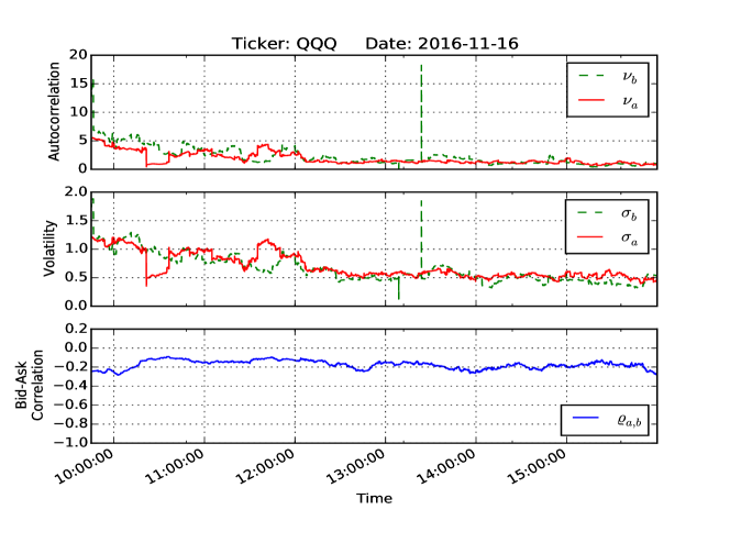
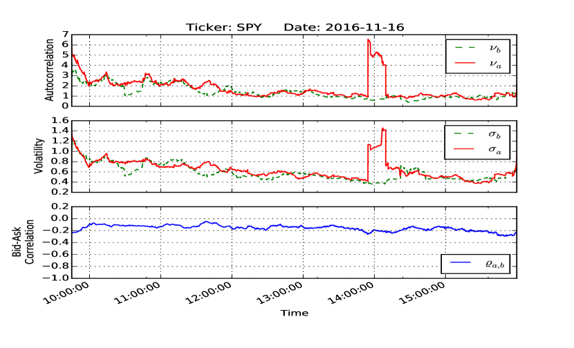
Figure 7. Autocorrelation ($\nu_{a/b}$), standard deviation ($\sigma_{a/b}$) and bid-ask correlation ($\varrho_{a,b}$) of order book depth in first 2 levels for two liquid ETFs (QQQ and SPY).

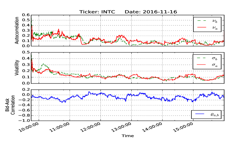
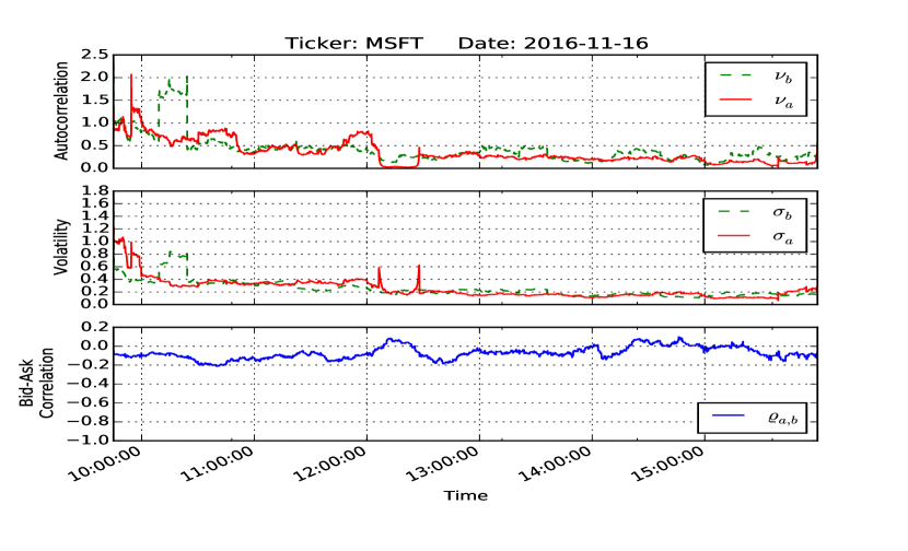
Figure 8. Autorcorrelation ($\nu_{a/b}$), standard deviation ($\sigma_{a/b}$) and bid-ask correlation ($\varrho_{a,b}$) of order book depth in first 2 levels for two liquid stocks (INTC and MSFT).

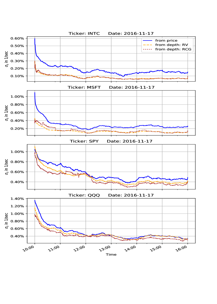
Figure 9. Comparison of various estimators for intraday price volatility $\sigma_{S}$: standard deviation of price changes (blue), estimator based on realized variance/covariance of bid/ask depth (red), and estimator based on martingale estimation function (orange).

Appendix A Dynamics in absolute price coordinates

We now discuss in more detail the generalized Itô-Wentzell formula for distribution-valued processes, which is used in Section 3.5 to derive the dynamics of the (non-centered) order book density $v_{t}(p)$. Let $C_{0}^{\infty}:=C_{0}^{\infty}(\mathbb{R})$ be the space of smooth compactly supported functions on $\mathbb{R}$, $\mathbb{D}$ its dual, the space of generalized functions. We denote by $\tfrac{\partial}{\partial x}$ and $\tfrac{\partial^{2}}{\partial x^{2}}$ the first two derivatives in the sense of distributions and by $\left\langle.,.\right\rangle$ the duality product on $\mathbb{D}\times C_{0}^{\infty}$.

A $\mathbb{D}$-valued stochastic process $u=(u_{t})_{t\geq 0}$ on a filtered probability space $(\Omega,\mathcal{F},\mathbb{F},\mathbb{P})$ is called $\mathbb{F}$-predictable if for all $\phi\in C^{\infty}_{0}(\mathbb{R})$ the real valued process $\left(\left\langle u_{t},\phi\right\rangle\right)_{t\geq 0}$ is predictable.

Let $N\in\mathbb{N}$ and $(b_{t})_{t\geq 0}$ and $(c_{t}^{k})_{t\geq 0}$, $k\in\{1,\ldots,N\}$ be predictable $\mathbb{D}$ valued processes. We assume that for all $T$, $R\in(0,\infty)$ and all $\phi\in C^{\infty}_{0}(\mathbb{R})$, almost surely

(A.1) $$\int_{0}^{T}\sup_{\left\lvert x\right\rvert\leq R}\left\lvert\left\langle b_{t},\phi(.-x)\right\rangle\right\rvert+\sum_{k=1}^{N}\left\lvert\left\langle c_{t}^{k},\phi(.-x)\right\rangle\right\rvert^{2}\,\operatorname{d}t<\infty.$$

Let $(W_{t}^{k},k=1,\ldots,N)_{t\geq 0}$ be independent scalar Brownian motions. We consider an equation of the form

(A.2) $$\,\operatorname{d}u_{t}=b_{t}\,\operatorname{d}t+\sum_{k=1}^{N}c_{t}^{k}\,\operatorname{d}W_{t}^{k},$$

Definition A.1.

A $\mathbb{D}$-valued stochastic process $(u_{t})_{t\geq 0}$ is called a solution of (A.2) in the sense of distributions with initial condition $u_{0}$ if for $t\in(0,\infty)$ and $\phi\in C^{\infty}_{0}$

(A.3) $$\left\langle u_{t},\phi\right\rangle-\left\langle u_{0},\phi\right\rangle=\int_{0}^{t}\left\langle b_{s},\phi\right\rangle\,\operatorname{d}t+\sum_{k=1}^{N}\int_{0}^{t}\left\langle c_{s}^{k},\phi\right\rangle{\,\operatorname{d}W_{s}^{k}}.$$

holds almost surely.

The following change of variable formula is a special case of a result by Krylov [Krylov, 2011, Theorem 1.1]:

Theorem A.2 (Generalized Itô-Wentzell formula).

Let $(u_{t})_{t\geq 0}$ be a solution of  (A.2) in the sense of distributions and let $(x_{t})_{t\geq 0}$ be a locally integrable process with representation

$$\,\operatorname{d}x_{t}=\mu_{t}\,\operatorname{d}t+\sum_{k=1}^{N}\sigma^{k}_{t}\,\operatorname{d}W_{t}^{k},\qquad t\geq 0.$$

where $(\mu_{t})_{t\geq 0}$ and $(\sigma^{k}_{t},k=1..N)_{t\geq 0}$ are real-valued predictable processes. Define the $\mathbb{D}$-valued process $(v_{t})_{t\geq 0}$ by $v_{t}(x):=u_{t}(x+x_{t})$, for $x\in\mathbb{R}$, $t\in[0,\infty)$. Then $(v_{t})_{t\geq 0}$ is a solution of

$$\,\operatorname{d}v_{t}=\left[b_{t}(.+x_{t})+\tfrac{1}{2}\left(\sum_{k=1}^{N}\left\lvert\sigma_{t}^{k}\right\rvert^{2}\right)\tfrac{\partial^{2}}{\partial x^{2}}v_{t}+\mu_{t}\tfrac{\partial}{\partial x}v_{t}+\sum_{k=1}^{N}\left(\sigma_{t}^{k}\tfrac{\partial}{\partial x}c_{t}^{k}(.+x_{t})\right)\right]\,\operatorname{d}t\\ +\sum_{k=1}^{N}\left[c_{t}^{k}(.+x_{t})+\sigma_{t}^{k}\tfrac{\partial}{\partial x}v_{t}\right]\,\operatorname{d}W_{t}^{k}$$

in the sense of distributions.

Remark A.3.

It is worth noting that the correlation of $(u_{t})$ and $(x_{t})$ contributes the term

$$\sum_{k=1}^{N}\left(\sigma_{t}^{k}\tfrac{\partial}{\partial x}c_{t}^{k}(.+x_{t})\right).$$

We now apply the above Itô-Wentzell formula in order to derive the dynamics of the order book density $v$, in non-centered coordinates, in the setting considered in Sections 3 and 4.

Let $L\in(0,\infty]$ and $I:=(-L,0)\cup(0,L)$. For $h$, $f\in H^{2}(I)\cap H^{1}_{0}(I)$. Then, (1.2) with initial condition $u_{0}=h$ admits a unique (analytically) strong solution denoted by $(u_{t})_{t\geq 0}$ . Let $\tilde{u}_{t}$ be the trivial extension of $u_{t}$ to $\mathbb{R}$, i. e.

(A.4) $$\tilde{u}_{t}(x):=\begin{cases}u_{t}(x),&x\in I,\\ 0,&\text{ otherwise}.\end{cases}$$

Note that $\tilde{u}\in H^{2}(\mathbb{R}\setminus\{-L,0,L\})\cap H^{1}(\mathbb{R})$. Recall that $\Delta$ and $\nabla$ in the previous discussions denoted the weak derivatives on $\mathbb{R}\setminus\{-L,0,L\}$, and we get that $\tfrac{\partial}{\partial x}\tilde{u}=\nabla\tilde{u}$ and

(A.5) $$\tfrac{\partial^{2}}{\partial x^{2}}\tilde{u}-\Delta\tilde{u} =\tfrac{\partial}{\partial x}\nabla\tilde{u}-\nabla\nabla\tilde{u}$$

$$=(\nabla\tilde{u}(-L+)-\nabla\tilde{u}(-L-))\delta_{-L}$$

$$+(\nabla\tilde{u}(0+)-\nabla\tilde{u}(0-))\delta_{0}+(\nabla\tilde{u}(L+)-\nabla\tilde{u}(L-))\delta_{L},$$

where $\delta_{x}$ denotes a point mass at $x\in\mathbb{R}$. Define

(A.6) $$b_{t}(x) :=\begin{cases}\eta_{a}\Delta u_{t}(x)+\beta_{a}\nabla u_{t}(x)+\alpha_{a}u_{t}(x)+f_{a}(x),&x\in(0,L),\\ \eta_{b}\Delta u_{t}(x)-\beta_{b}\nabla u_{t}(x)+\alpha_{b}u_{t}(x)-f_{b}(x),&x\in(-L,0),\\ 0,&\text{ otherwise},\end{cases}$$

(A.7) $$c_{t}^{1}(x) :=\begin{cases}\sigma_{a}\varrho_{a,b}u_{t}(x),&x\in(0,L),\\ \sigma_{b}u_{t}(x),&x\in(-L,0),\\ 0,&\text{ otherwise},\end{cases}$$

(A.8) $$c_{t}^{2}(x) :=\begin{cases}\sigma_{a}\sqrt{1-\varrho_{a,b}^{2}}u_{t}(x),&x\in(0,L),\\ 0,&\text{ otherwise},\end{cases}$$

so that

(A.9) $$\,\operatorname{d}\tilde{u}_{t}=b_{t}\,\operatorname{d}t+c_{t}^{1}\,\operatorname{d}W_{t}^{1}+c_{t}^{2}\,\operatorname{d}W_{t}^{2}.$$

The Cauchy-Schwartz inequality shows that (A.1) is satisfied. Assume now that the mid price $(S_{t})_{t\geq 0}$ follows the dynamics

(A.10) $$\,\operatorname{d}S_{t}=c_{s}\theta\mu_{t}\,\operatorname{d}t+c_{s}\theta(\sigma_{b}-\sigma_{a}\varrho_{a,b})\,\operatorname{d}W_{t}^{1}-c_{s}\theta\sigma_{a}\sqrt{1-\varrho_{a,b}^{2}}\,\operatorname{d}W_{t}^{2}.$$

for some integrable predictable process $\mu$. Define

(A.11) $$\sigma_{s}:=c_{s}\theta\sqrt{\sigma_{b}^{2}+\sigma_{a}^{2}-2\varrho_{a,b}\sigma_{b}\sigma_{a}}.$$

Then, Theorem A.2 yields that for $v_{t}(x):=\tilde{u}_{t}(x-S_{t})$ we get

(A.12) $$\,\operatorname{d}v_{t} =\left[b_{t}(.-S_{t})+\tfrac{1}{2}\sigma_{s}^{2}\tfrac{\partial^{2}}{\partial x^{2}}v_{t}-c_{s}\theta\mu_{t}\tfrac{\partial}{\partial x}v_{t}\right.$$

$$\qquad\left.-\left(c_{s}\theta\left(\sigma_{b}-\varrho_{a,b}\sigma_{a}\right)\tfrac{\partial}{\partial x}c_{t}^{1}(.-S_{t})+c_{s}\theta\sqrt{1-\varrho_{a,b}^{2}}\sigma_{a}\tfrac{\partial}{\partial x}c_{t}^{2}(.-S_{t})\right)\right]\,\operatorname{d}t$$

$$\qquad+\left(c_{t}^{1}(.-S_{t})-c_{s}\theta\left(\sigma_{b}-\varrho_{a,b}\sigma_{a}\right)\tfrac{\partial}{\partial x}v_{t}\right)\,\operatorname{d}W_{t}^{1}$$

$$\qquad+\left(c_{t}^{2}(.-S_{t})+c_{s}\theta\sqrt{1-\varrho_{a,b}^{2}}\sigma_{a}\tfrac{\partial}{\partial x}v_{t}\right)\,\operatorname{d}W_{t}^{2}$$

i. e. $v$ is a solution of the stochastic moving boundary problem,

(A.13) $$\,\operatorname{d}v_{t} =\left[\left(\eta_{a}+\tfrac{1}{2}\sigma_{s}^{2}\right)\Delta v_{t}+\left(\beta_{a}-c_{s}\theta\mu_{t}-c_{s}\theta\left(\varrho_{a,b}\sigma_{b}\sigma_{a}-\sigma_{a}^{2}\right)\right)\nabla v_{t}\right.$$

$$\qquad\hskip 120.00018pt\left.\vphantom{\left(\eta_{a}+\tfrac{1}{2}\sigma_{s}^{2}\right)\Delta v_{t}+\left(\beta_{a}-c_{s}\theta\mu_{t}-c_{s}\theta\left(\varrho_{a,b}\sigma_{b}\sigma_{a}-\sigma_{a}^{2}\right)\right)\nabla v_{t}}+\alpha_{a}v_{t}+f_{a}(.-S_{t})\right]\,\operatorname{d}t$$

$$\quad+\left(\sigma_{a}\varrho_{a,b}v_{t}-c_{s}\theta\left(\sigma_{b}-\varrho_{a,b}\sigma_{a}\right)\nabla v_{t}\right)\,\operatorname{d}W_{t}^{1}$$

$$\quad+\sigma_{a}\sqrt{1-\varrho_{a,b}^{2}}\left(v_{t}+c_{s}\theta\nabla v_{t}\right)\,\operatorname{d}W_{t}^{2},\ \text{ on }\ (S_{t},S_{t}+L),$$

$$\,\operatorname{d}v_{t} =\left[\left(\eta_{b}+\tfrac{1}{2}\sigma_{s}^{2}\right)\Delta v_{t}-\left(\beta_{b}+c_{s}\theta\mu_{t}+c_{s}\theta\left(\sigma_{b}^{2}-\varrho_{a,b}\sigma_{b}\sigma_{a}\right)\right)\nabla v_{t}\right.$$

$$\qquad\hskip 120.00018pt\left.\vphantom{\left(\eta_{b}+\tfrac{1}{2}\sigma_{s}^{2}\right)\Delta v_{t}\left(\beta_{b}+c_{s}\theta\mu_{t}+c_{s}\theta\left(\sigma_{b}^{2}-\varrho_{a,b}\sigma_{b}\sigma_{a}\right)\right)\nabla v_{t}}+\alpha_{b}v_{t}-f_{b}(.-S_{t})\right]\,\operatorname{d}t$$

$$\quad+\left(\sigma_{b}v_{t}-c_{s}\theta\left(\sigma_{b}-\varrho_{a,b}\sigma_{a}\right)\nabla v_{t}\right)\,\operatorname{d}W_{t}^{1}$$

$$\quad+c_{s}\theta\sqrt{1-\varrho_{a,b}^{2}}\sigma_{a}\nabla v_{t}\,\operatorname{d}W_{t}^{2}\ \text{ on }\ (S_{t}-L,S_{t}),$$

$$v_{t} =0\qquad\text{ otherwise;}$$

$$\,\operatorname{d}S_{t} =c_{s}\theta\mu_{t}\,\operatorname{d}t+c_{s}\theta(\sigma_{b}-\varrho_{a,b}\sigma_{a})\,\operatorname{d}W_{t}^{1}-c_{s}\theta\sqrt{1-\varrho_{a,b}^{2}}\sigma_{a}\,\operatorname{d}W_{t}^{2},$$

To define what we mean by solution in this context we introduce the mappings

$$\mathbb{L}\colon\bigcup_{x\in\mathbb{R}}\left[\left(H^{2}(\mathbb{R}\setminus\{x-L,x,x+L\})\cap H^{1}_{0}(\mathbb{R}\setminus\{x-L,x,x+L\})\right)\times\{x\}\right]\to\mathbb{D},$$

$$\quad(v,s) \mapsto(\nabla(v(s-L+)-\nabla v(s-L-)))\delta_{s-L}$$

$$\qquad+(\nabla(v(s+)-\nabla v(s-)))\delta_{s}$$

$$\qquad+(\nabla(v(s+L+)-\nabla v(s+L-)))\delta_{s+L}.$$

Define now the functions $\bar{\mu}\colon\mathbb{R}^{5}\to\mathbb{R}$, $\bar{\sigma}_{1}$, $\bar{\sigma}_{2}\colon\mathbb{R}^{4}\to\mathbb{R}$ as

$$\bar{\mu}(x,y^{\prime\prime},y^{\prime},y,s) :=\begin{cases}(\eta_{a}+\tfrac{1}{2}\sigma_{s}^{2})y^{\prime\prime}+(\beta_{a}-c_{s}\theta(\varrho_{a,b}\sigma_{b}\sigma_{a}-\sigma_{a}^{2}))y^{\prime}&\\ \hfill+\alpha_{a}y+f_{a}(x),&x\in(0,L)\\ (\eta_{b}+\tfrac{1}{2}\sigma_{s}^{2})y^{\prime\prime}-(\beta_{a}+c_{s}\theta(\sigma_{b}^{2}-\varrho_{a,b}\sigma_{b}\sigma_{a}))y^{\prime}&\\ \hfill+\alpha_{b}y-f_{b}(x),&x\in(-L,0),\\ 0,&\text{ otherwise},\end{cases}$$

$$\bar{\sigma}_{1}(x,y^{\prime},y,s) :=\begin{cases}\sigma_{a}\varrho_{a,b}y,&x\in(0,L),\\ \sigma_{b}y,&x\in(-L,0),\\ 0,&\text{ otherwise},\end{cases}$$

$$\bar{\sigma}_{2}(x,y^{\prime},y,s) :=\begin{cases}\sigma_{a}\sqrt{1-\varrho_{a,b}^{2}}y,&x\in(0,L)\\ 0,\quad\text{ otherwise}&\end{cases}$$

for $x$, $y^{\prime\prime}$, $y^{\prime}$, $y$, $s\in\mathbb{R}$.

Following [Mueller, 2018, Definition 1.11], a solution of (A.13) is an $L^{2}(\mathbb{R})\times\mathbb{R}$-continuous stochastic process $(v_{t},S_{t})$, taking values in

$$\bigcup_{x\in\mathbb{R}}\left[\left(H^{2}(\mathbb{R}\setminus\{x-L,x,x+L\})\cap H^{1}_{0}(\mathbb{R}\setminus\{x-L,x,x+L\})\right)\times\{x\}\right],$$

such that $(S_{t})$ is given by (A.10) and, in the sense of distributions,

(A.14) $$\,\operatorname{d}v_{t}=\left(\bar{\mu}(.-S_{t},\Delta v_{t},\nabla v_{t},v_{t},S_{t})\right)\,\operatorname{d}t-\nabla v_{t}\,\operatorname{d}S_{t}+\tfrac{1}{2}\mathbb{L}(v_{t},S_{t})\,\operatorname{d}\langle S\rangle_{t}\\ +\bar{\sigma}_{1}(.-S_{t},\nabla v_{t},v_{t},S_{t})\,\operatorname{d}W_{t}^{1}+\bar{\sigma}_{2}(.-S_{t},\nabla v_{t},v_{t},S_{t})\,\operatorname{d}W_{t}^{2}.$$

References

[Bibby et al., 2005]
Bibby, B. M., Skovgaard, I. M., and Sørensen, M. (2005).
Diffusion-type models with given marginal distribution and
autocorrelation function.
Bernoulli, 11(2):191–220.
[Bibby and Sørensen, 1995]
Bibby, B. M. and Sørensen, M. (1995).
Martingale estimation functions for discretely observed diffusion
processes.
Bernoulli, 1(1-2):17–39.
[Borodin and Salminen, 2012]
Borodin, A. N. and Salminen, P. (2012).
Handbook of Brownian motion-facts and formulae.
Birkhäuser.
[Bouchaud et al., 2009]
Bouchaud, J.-P., Farmer, J., and Lillo, F. (2009).
How markets slowly digest changes in supply and demand.
In Hens, T. and Schenk-Hoppe, K. R., editors, Handbook of
financial markets: dynamics and evolution, pages 57–160. Elsevier.
[Burger et al., 2013]
Burger, M., Caffarelli, L., Markowich, P. A., and Wolfram, M.-T. (2013).
On a Boltzmann-type price formation model.
Proceedings of the Royal Society of London A: Mathematical,
Physical and Engineering Sciences, 469(2157).
[Caffarelli et al., 2011]
Caffarelli, L. A., Markowich, P. A., and Pietschmann, J.-F. (2011).
On a price formation free boundary model by Lasry and Lions.
Comptes Rendus Mathematique, 349(11):621 – 624.
[Carmona and Webster, 2013]
Carmona, R. and Webster, K. (2013).
The Self-Financing Equation in High Frequency Markets.
ArXiv 1312.2302.
[Cartea et al., 2018]
Cartea, A., Donnelly, R., and Jaimungal, S. (2018).
Enhancing trading strategies with order book signals.
Applied Mathematical Finance, 25(1):1–35.
[Chavez-Casillas and Figueroa-Lopez, 2017]
Chavez-Casillas, J. A. and Figueroa-Lopez, J. (2017).
A one-level limit order book model with memory and variable spread.
Stochastic Processes and their Applications, 127(8):2447 –
2481.
[Chayes et al., 2009]
Chayes, L., del Mar Gonzalez, M., Gualdani, M., and Kim, I. (2009).
Global existence and uniqueness of solutions to a model of price
formation.
SIAM Journal on Mathematical Analysis, 41(5):2107–2135.
[Cont, 2005]
Cont, R. (2005).
Modeling term structure dynamics: an infinite dimensional approach.
Int. Journal of Theoretical and Applied finance,
8(03):357–380.
[Cont, 2011]
Cont, R. (2011).
Statistical modeling of high-frequency financial data.
IEEE Signal Processing, 28(5):16–25.
[Cont and De Larrard, 2012]
Cont, R. and De Larrard, A. (2012).
Order book dynamics in liquid markets: Limit theorems and diffusion
approximations.
[Cont and de Larrard, 2013]
Cont, R. and de Larrard, A. (2013).
Price dynamics in a Markovian limit order market.
SIAM J. Financial Math., 4(1):1–25.
[Cont et al., 2014]
Cont, R., Kukanov, A., and Stoikov, S. (2014).
The price impact of order book events.
Journal of Financial Econometrics, 12(1):47–88.
[Cont and Mueller, 2018]
Cont, R. and Mueller, M. (2018).
LOBPY Python package: https://github.com/mm842/lobpy.
[Cont et al., 2010]
Cont, R., Stoikov, S., and Talreja, R. (2010).
A stochastic model for order book dynamics.
Oper. Res., 58(3):549–563.
[Da Prato and Zabczyk, 2014]
Da Prato, G. and Zabczyk, J. (2014).
Stochastic equations in infinite dimensions.
Cambridge University Press, 2nd edition.
[Evans, 2010]
Evans, L. C. (2010).
Partial Differential Equations, volume 19.
American Mathematical Society, 2nd edition.
[Filipovic and Teichmann, 2003]
Filipovic, D. and Teichmann, J. (2003).
Existence of invariant manifolds for stochastic equations in infinite
dimension.
Journal of Functional Analysis, 197(2):398 – 432.
[Forman and Sørensen, 2008]
Forman, J. L. and Sørensen, M. (2008).
Pearson diffusions: A class of statistically tractable diffusion
processes.
Scandinavian Journal of Statistics, 35(3):438–465.
[Gaspar, 2006]
Gaspar, R. (2006).
Finite dimensional Markovian realizations for forward price term
structure models.
In Shiryaev, A., Grossinho, M., Oliveira, P., and Esquivel, M.,
editors, Stochastic Finance, pages 265–320. Springer.
[Hambly et al., 2020]
Hambly, B., Kalsi, J., and Newbury, J. (2020).
Limit order books, diffusion approximations and reflected SPDEs:
From microscopic to macroscopic models.
Applied Mathematical Finance, 27(1-2):132–170.
[Horst and Kreher, 2018]
Horst, U. and Kreher, D. (2018).
Second order approximations for limit order books.
Finance and Stochastics, 22(4):827–877.
[Huang et al., 2017]
Huang, W., Lehalle, C.-A., and Rosenbaum, M. (2017).
Simulating and analyzing order book data: The queue-reactive model.
Journal of the American Statistical Association, 110:107–122.
[Kallenberg, 2002]
Kallenberg, O. (2002).
Foundations of Modern Probability.
Springer.
[Karatzas and Kardaras, 2007]
Karatzas, I. and Kardaras, C. (2007).
The numéraire portfolio in semimartingale financial models.
Finance and Stochastics, 11(4):447–493.
[Karatzas and Shreve, 1987]
Karatzas, I. and Shreve, S. (1987).
Brownian motion and stochastic calculus.
Springer.
[Kelly and Yudovina, 2018]
Kelly, F. and Yudovina, E. (2018).
A Markov model of a limit order book: Thresholds, recurrence, and
trading strategies.
Mathematics of Operations Research, 43(1):181–203.
[Kirilenko et al., 2017]
Kirilenko, A., Kyle, A., Samadi, M., and Tuzun, T. (2017).
The flash crash: High frequency trading on an electronic market.
Journal of Finance, LXXII:967–998.
[Kloeden and Platen, 1992]
Kloeden, P. E. and Platen, E. (1992).
Numerical Solution of Stochastic Differential Equations.
Springer.
[Krylov, 2011]
Krylov, N. V. (2011).
On the Itô-Wentzell formula for distribution-valued processes
and related topics.
Probab. Theory Related Fields, 150(1-2):295–319.
[Lasry and Lions, 2007]
Lasry, J.-M. and Lions, P.-L. (2007).
Mean field games.
Jpn. J. Math., 2(1):229–260.
[Lehalle and Laruelle, 2018]
Lehalle, C.-A. and Laruelle, S. (2018).
Market microstructure in practice.
World Scientific.
[Leonenko and Šuvak, 2010]
Leonenko, N. and Šuvak, N. (2010).
Statistical inference for reciprocal gamma diffusion process.
Journal of statistical planning and inference, 140(1):30–51.
[Lévine, 1991]
Lévine, J. (1991).
Finite dimensional realizations of stochastic PDEs and application
to filtering.
Stochastics and Stochastic Reports, 37(1-2):75–103.
[Lipton et al., 2014]
Lipton, A., Pesavento, U., and Sotiropoulos, M. G. (2014).
Trading strategies via book imbalance.
RISK, pages 70–75.
[Luckock, 2003]
Luckock, H. (2003).
A steady-state model of the continuous double auction.
Quantitative Finance, 3(5):385–404.
[Markowich et al., 2016]
Markowich, P., Teichmann, J., and Wolfram, M. (2016).
Parabolic free boundary price formation models under market size
fluctuations.
Multiscale Modeling & Simulation, 14(4):1211–1237.
[Milian, 2002]
Milian, A. (2002).
Comparison theorems for stochastic evolution equations.
Stoch. Stoch. Rep., 72(1-2):79–108.
[Mueller, 2018]
Mueller, M. S. (2018).
A stochastic Stefan-type problem under first-order boundary
conditions.
The Annals of Applied Probability, 28(4):2335–2369.
[Revuz and Yor, 1999]
Revuz, D. and Yor, M. (1999).
Continuous Martingales and Brownian Motion.
Springer.
[Schlichting and Gersten, 2017]
Schlichting, H. and Gersten, K. (2017).
Boundary-layer theory.
Graduate Texts in Mathematics. Springer-Verlag.
[Smith et al., 2003]
Smith, E., Farmer, J. D., Gillemot, L., and Krishnamurthy, S. (2003).
Statistical theory of the continuous double auction.
Quantitative Finance, 3(6):481–514.
[Yosida, 1995]
Yosida, K. (1995).
Functional analysis.
Classics in Mathematics. Springer.