An Experimental Study of Algorithms for Geodesic Shortest Paths in the Constant-Workspace Model

Abstract

We perform an experimental evaluation of algorithms for finding geodesic shortest paths between two points inside a simple polygon in the constant-workspace model. In this model, the input resides in a read-only array that can be accessed at random. In addition, the algorithm may use a constant number of words for reading and for writing. The constant-workspace model has been studied extensively in recent years, and algorithms for geodesic shortest paths have received particular attention.

We have implemented three such algorithms in Python, and we compare them to the classic algorithm by Lee and Preparata that uses linear time and linear space. We also clarify a few implementation details that were missing in the original description of the algorithms. Our experiments show that all algorithms perform as advertised in the original works and according to the theoretical guarantees. However, the constant factors in the running times turn out to be rather large for the algorithms to be fully useful in practice.

1 Introduction

In recent years, the constant-workspace model has enjoyed growing popularity in the computational geometry community [6]. Motivated by the increasing deployment of small devices with limited memory capacities, the goal is to develop simple and efficient algorithms for the situation where little workspace is available. The model posits that the input resides in a read-only array that can be accessed at random. In addition, the algorithm may use a constant number of memory words for reading and for writing. The output must be written to a write-only memory that cannot be accessed again for reading. Following the initial work by Asano et al. from 2011 [2], numerous results have been published for this model, leading to a solid theoretical foundation for dealing with geometric problems when the working memory is scarce. The recent survey by Banyassady et al. [6] gives an overview of the problems that have been considered and of the results that are available for them.

But how do these theoretical results measure up in practice, particularly in view of the original motivation? To investigate this question, we have implemented three different constant-workspace algorithms for computing geodesic shortest paths in simple polygons. This is one of the first problems to be studied in the constant-workspace model [2, 3]. Given that the general shortest path problem is unlikely to be amenable to constant-workspace algorithms (it is NL-complete [18]), it may come as a surprise that a solution for the geodesic case exists at all. By now, several algorithms are known, both for constant workspace as well as in the time-space-trade-off regime, where the number of available cells of working memory may range from constant to linear [1, 12].

Due to the wide variety of approaches and the fundamental nature of the problem, geodesic shortest paths are a natural candidate for a deeper experimental study. Our experiments show that all three constant-workspace algorithms work well in practice and live up to their theoretical guarantees. However, the large running times make them ill-suited for very large input sizes. During our implementation, we also noticed some missing details in the original publications, and we explain below how we have dealt with them.

As far as we know, our study constitutes the first large-scale comparative evaluation of geometric algorithms in the constant-workspace model. A previous implementation study, by Baffier et al. [5], focused on time-space trade-offs for stack-based algorithms and was centered on different applications of a powerful algorithmic technique. Given the practical motivation and wide applicability of constant-workspace algorithms for geometric problems, we hope that our work will lead to further experimental studies in this direction.

2 The Four Shortest-Path Algorithms

We provide a brief summary for each of the four algorithms in our implementation; further details can be found in the original papers [3, 2, 14]. In each case, we use $P$ to denote a simple input polygon in the plane with $n$ vertices. We consider $P$ to be a closed, connected subset of the plane. Given two points $s,t\in P$, our goal is to compute a shortest path from $s$ to $t$ (with respect to the Euclidean length) that lies completely inside $P$.

2.1 The Classic Algorithm by Lee and Preparata

This is the classic linear-space algorithm for the geodesic shortest path problem that can be found in textbooks [14, 11]. It works as follows: we triangulate $P$, and we find the triangle that contains $s$ and the triangle that contains $t$. Next, we determine the unique path between these two triangles in the dual graph of the triangulation. The path is unique since the dual graph of a triangulation of a simple polygon is a tree [7]. We obtain a sequence $e_{1},\dots,e_{m}$ of diagonals (incident to pairs of consecutive triangles on the dual path) crossed by the geodesic shortest path between $s$ and $t$, in that order. The algorithm walks along these diagonals, while maintaining a funnel. The funnel consists of a cusp $p$, initialized to be $s$, and two concave chains from $p$ to the two endpoints of the current diagonal $e_{i}$. An example of these funnels can be found in Fig. 1. In each step $i$ of the algorithm, $i=1,\dots,m-1$, we update the funnel for $e_{i}$ to the funnel for $e_{i+1}$. There are two cases: (i) if $e_{i+1}$ remains visible from the cusp $p$, we update the appropriate concave chain, using a variant of Graham’s scan; (ii) if $e_{i+1}$ is no longer visible from $p$, we proceed along the appropriate chain until we find the cusp for the next funnel. We output the vertices encountered along the way as part of the shortest path.

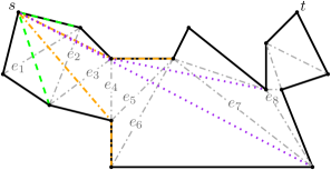
Figure 1: Examples of three funnels during the algorithm for finding a shortest path from $s$ to $t$. Each has cusp $s$ and goes up to diagonals $e_{2}$ (green, dashed), $e_{6}$ (orange, dash dotted), and $e_{8}$ (purple, dotted).

Implemented in the right way, this procedure takes linear time and space.

2.2 Using Constrained Delaunay-Triangulations

The first constant-workspace-algorithm for geodesic shortest paths in simple polygons was presented by Asano et al. [3] in 2011. It is called Delaunay, and it constitutes a relatively direct adaptation of the method of Lee and Preparata to the constant-workspace model.

In the constant-workspace model, we cannot explicitly compute and store a triangulation of $P$. Instead, we use a uniquely defined implicit triangulation of $P$, namely the constrained Delaunay triangulation of $P$ [9]. In this variant of the classic Delaunay triangulation, we prescribe the edges of $P$ to be part of the desired triangulation. Then, the additional triangulation edges cannot cross the prescribed edges. Thus, unlike in the original Delaunay triangulation, the circumcircle of a triangle may contain other vertices of $P$, as long as the line segment from a triangle endpoint to the vertex crosses a prescribed polygon edge, see Fig. 2 for an example.

(a) The Delaunay triangulation of a point set.

(b) A polygon on the point set which intersects the triangulation.

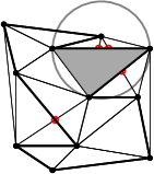
(c) The circumcircle may contain points not visible from some triangle vertices.

Figure 2: An example of a constrained Delaunay triangulation of a simple polygon.

The constrained Delaunay triangulation of $P$ can be navigated efficiently using constant workspace: given a diagonal or a polygon edge, we can find the two incident triangles in $O(n^{2})$ time [3]. Using an $O(n)$ time constant-workspace-algorithm for finding shortest paths in trees, also given by Asano et al. [3], we can thus enumerate all triangles in the dual path between the constrained Delaunay triangle that contains $s$ and the constrained Delaunay triangle that contains $t$ in $O(n^{3})$ time.

As in the algorithm by Lee and Preparata, we need to maintain the visibility funnel while walking along the dual path of the constrained Delaunay triangulation. Instead of the complete chains, we store only the two line segments that define the current visibility cone (essentially the cusp together with the first vertex of each chain). We recompute the two chains whenever it becomes necessary. The total running time of the algorithm is $O(n^{3})$. More details can be found in the paper by Asano et al. [3].

2.3 Using Trapezoidal Decompositions

This algorithm was also proposed by Asano et al. [3], as a faster alternative to the algorithm that uses constrained Delaunay triangulations. It is based on the same principle as Delaunay, but it uses the trapezoidal decomposition of $P$ instead of the Delaunay triangulation [7]. See Fig. 3 for a depiction of the decomposition and the symbolic perturbation method to avoid a general position assumption. In the algorithm, we compute a trapezoidal decomposition of $P$, and we follow the dual path between the trapezoid that contains $s$ and the trapezoid that contains $t$, while maintaining a funnel and outputting the new vertices of the geodesic shortest path as they are discovered. Assuming general position, we can find all incident trapezoids of the current trapezoid and determine how to continue on the way to $t$ in $O(n)$ time (instead of $O(n^{2})$ time in the case of the Delaunay algorithm). Since there are still $O(n)$ steps, the running time improves to $O(n^{2})$.

(a) The trapezoidal decomposition is obtained by shooting rays up and down at every vertex.

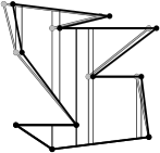
(b) Shifting all points to the right by $y\varepsilon$ makes sure no two share the same $x$-coordinate.

Figure 3: The trapezoidal decomposition of a polygon. If the polygon is in general position (right) each trapezoid has at most four neighbors which can all be found in $O(n)$ time.

2.4 The Makestep Algorithm

This algorithm was presented by Asano et al. [2]. It uses a direct approach to the geodesic shortest path problem and unlike the two previous algorithms, it does not try to mimic on the algorithm by Lee and Preparata. In the traditional model, this approach would be deemed too inefficient, but in the constant-workspace world, its simplicity turns out to be beneficial. The main idea is as follows: we maintain a current vertex $p$ of the geodesic shortest path, together with a visibility cone, defined by two points $q_{1}$ and $q_{2}$ on the boundary of $P$. The segments $pq_{1}$ and $pq_{2}$ cut off a subpolygon $P^{\prime}\subseteq P$. We maintain the invariant that the target $t$ lies in $P^{\prime}$. In each step, we gradually shrink $P^{\prime}$ by advancing $q_{1}$ and $q_{2}$, sometimes also relocating $p$ and outputting a new vertex of the geodesic shortest path. These steps are illustrated in Fig. 4. It is possible to realize the shrinking steps in such a way that there are only $O(n)$ of them. Each shrinking step takes $O(n)$ time, so the total running time of the MakeStep algorithm is $O(n^{2})$.

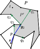
(a) $P^{\prime}$ is the subset of $P$ cut off by the three points $p$, $q_{1}$, and $q_{2}$. Both points are convex, one is advanced.

(b) Since $q_{2}$ is reflex we shoot a ray until it hits the boundary. $t$ lies to the left of this ray.

(c) $p$ is relocated to the previous position of $q_{2}$ and $P^{\prime}$ is shrunk along the ray.

Figure 4: An illustration of the steps in the Makestep algorithm.

3 Our Implementation

We have implemented the four algorithms from Section 2 in Python [15]. For graphical output and for plots, we use the matplotlib library [13]. Even though there are some packages for Python that provide geometric objects such as line segments, circles, etc., none of them seemed suitable for our needs. Thus, we decided to implement all geometric primitives on our own. The source code of the implementation is available online in a Git-repository.

In order to apply the algorithm Lee-Preparata, we must be able to triangulate the simple input polygon $P$ efficiently. Since implementing an efficient polygon triangulation algorithm can be challenging and since this is not the main objective of our study, we relied for this on the Python Triangle library by Rufat [16], a Python wrapper for Shewchuk’s Triangle, which was written in C [17]. We note that Triangle does not provide a linear-time triangulation algorithm, which would be needed to achieve the theoretically possible linear running time for the shortest path algorithm. Instead, it contains three different implementations, namely Fortune’s sweep line algorithm, a randomized incremental construction, and a divide-and-conquer method. All three implementations give a running time of $O(n\log{n})$. For our study, we used the divide-and conquer algorithm, the default choice. In the evaluation, we did not include the triangulation phase in the time and memory measurement for running the algorithm by Lee and Preparata.

3.1 General Implementation Details

All three constant-workspace algorithms have been presented with a general position assumption: Delaunay and Makestep assume that no three vertices lie on a line, while Trapezoid assumes that no two vertices have the same $x$-coordinate. Our implementations of Delaunay and Makestep also assume general position, but they throw exceptions if a non-recoverable general position violation is encountered. Most violations, however, can be dealt with easily in our code; e.g. when trying to find the constrained Delaunay triangle(s) for a diagonal, we can simply ignore points collinear to this diagonal. For the case of Trapezoid, Asano et al. [3] described how to enforce the general position assumption by changing the $x$-coordinate of every vertex to $x+\varepsilon y$ for some small enough $\varepsilon>0$ such that the $x$-order of all vertices is maintained. In our implementation, we apply this method to every polygon in which two vertices share the same $x$-coordinate.

The coordinates are stored as $64\text{\,}\mathrm{bit}$ IEEE 754 floats. In order to prevent problems with floating point precision or rounding, we take the following steps: first, we never explicitly calculate angles, but we rely on the usual three-point-orientation test, i.e., the computation of a determinant to find the position of a point $c$ relative to the directed line through to points $a$ and $b$ [7]. Second, if an algorithm needs to place a point somewhere in the relative interior of a polygon edge, we store an additional edge reference to account for inaccuracies when calculating the new point’s coordinates.

3.2 Implementing the Algorithm by Lee and Preparata

The algorithm by Lee and Preparata can be implemented easily, in a straightforward fashion. There are no particular edge cases or details that we need to take care of. Disregarding the code for the geometric primitives, the algorithm needs less then half as many lines of code than the other algorithms.

3.3 Implementing Delaunay and Trapezoid

Figure 5: During the gift wrapping from the cusp to the diagonal $b$, the vertices need to be restricted to the shaded area. Otherwise, $u$ would be considered to be part of the geodesic shortest path, as it is to the left of $vw$.

In both constant-workspace adaptations of the algorithm by Lee and Preparata, we encounter the following problem: whenever the cusp of the current funnel changes, we need to find the cusp of the new funnel, and we need to find the piece of the geodesic shortest path that connects the former cusp to the new cusp. In their description of the algorithm, Asano et al. [3] only say that this should be done with an application of gift wrapping (Jarvis’ march) [7]. While implementing these two algorithms, we noticed that a naive gift wrapping step that considers all the vertices on $P$ between the cusp of the current funnel and the next diagonal might include vertices that are not visible inside the polygon. Figure 5 shows an example: here $b$ is the next diagonal, and naively we would look at all vertices along the polygon boundary between $v$ and $w$. Hence, $u$ would be considered as a gift wrapping candidate, and since it forms the largest angle with the cusp and $v$ (in particular, an angle that is larger than the angle formed by $w$) it would be chosen as the next point, even though $w$ should be the cusp of the next funnel. A simple fix for this problem would be an explicit check for visibility in each gift-wrapping step. Unfortunately, the resulting increase in the running time would be too expensive for a realistic implementation of the algorithms.

Our solution for Trapezoid is to consider only vertices whose $x$-coordinate is between the cusp of the current vertex and the point where the current visibility cone crosses the boundary of $P$ for the first time. For ease of implementation, one can also limit it to the $x$-coordinate of the last trapezoid boundary visible from the cusp. Figure 5 shows this as the dotted green region. For Delaunay, a similar approach can be used. The only difference is that the triangle boundaries in general are not vertical lines.

3.4 Implementing Makestep

Our implementation of the Makestep algorithm is also relatively straightforward. Nonetheless, we would like to point out one interesting detail; see Fig. 6. The description by Asano et al. [2] says that to advance the visibility cone, we should check if “$t$ lies in the subpolygon from $q^{\prime}$ to $q_{1}$.” If so, the visibility cone should be shrunk to $q^{\prime}pq_{1}$, otherwise to $q_{2}pq^{\prime}$.

However, the “subpolygon from $q^{\prime}$ to $q_{1}$” is not clearly defined for the case that the line segment $q^{\prime}q_{1}$ is not contained in $P$. To avoid this difficulty, we instead consider the line segment $pq^{\prime}$. This line segment is always contained in $P$, and it divides the cutoff region $P^{\prime}$ into two parts, a “subpolygon” between $q^{\prime}$ and $q_{1}$ and a “subpolygon” between $q_{2}$ and $q^{\prime}$. Now we can easily choose the one containing $t$.

Figure 6: Left: Asano et al. [2] state that one should check whether “$t$ lies in the subpolygon from $q^{\prime}$ to $q_{1}$.” This subpolygon, however, is not clearly defined as the line segment $q^{\prime}q_{1}$ does not lie inside $P$. Considering $pq^{\prime}$ instead and using $q_{1}pq^{\prime}$ to shrink the cutoff region gives the correct result on the right.

4 Experimental Setup

We now describe how we conducted the experimental evaluation of our four implementations for geodesic shortest path algorithms.

4.1 Generating the Test Instances

Our experimental approach is as follows: given a desired number of vertices $n$, we generate 4–10 (pseudo)random polygons with $n$ vertices. For this, we use a tool developed in a software project carried out under the supervision of Günter Rote at the Institute of Computer Science at Freie Universität Berlin [10]. Among others, the tool provides an implementation of the Space Partitioning algorithm for generating random simple polygons presented by Auer and Held [4].

Next, we generate the set $S$ of desired endpoints for the geodesic shortest paths. This is done as follows: for each edge $e$ of each generated polygon, we find the incident triangle $t_{e}$ of $e$ in the constrained Delaunay triangulation of the polygon. We add the barycenter of $t_{e}$ to $S$. In the end, the set $S$ will have between $\left\lfloor n/2\right\rfloor$ and $n-2$ points. We will compute the geodesic shortest path for each pair of distinct points in $S$.

4.2 Executing the Tests

For each pair of points $s,t\in S$, we find the geodesic shortest path between $s$ and $t$ using each of the four implemented algorithms. Since the number of pairs grows quadratically in $n$, we restrict the tests to $1500$ random pairs for all $n\geq 200$.

First, we run each algorithm once in order to assess the memory consumption. This is done by using the get_traced_memory function of the built-in tracemalloc module which returns the peak and current memory consumption—the difference tells us how much memory was used by the algorithm. Starting the memory tracing just before running the algorithm gives the correct values for the peak memory consumption. In order to obtain reproducible numbers we also disable Python’s garbage collection functionality using the built-in gc.disable and gc.enable functions.

After that, we run the algorithm between $5$ and $20$ times, depending on how long it takes. We measure the processor time for each run with the process_time function of the time module which gives the time during which the process was active on the processor in user and in system mode. We then take the median of the times as a representative running time for this point pair.

4.3 Test Environment

Since we have a quadratic number of test cases for each instance, our experiments take a lot of time. Thus, the tests were distributed on multiple machines and on multiple cores. We had six computing machines at our disposal, each with two quad-core CPUs. Three machines had Intel Xeon E5430 CPUs with $2.67\text{\,}\mathrm{GHz}$; the other three had AMD Opteron 2376 CPUs with $2.3\text{\,}\mathrm{GHz}$. All machines had $32\text{\,}\mathrm{GB}$ RAM, even though, as can be seen in the next section, memory was never an issue. The operating system was a Debian 8 and we used version 3.5 of the Python interpreter to implement the algorithms and to execute the tests.

5 Experimental Results

Figure 7: Memory consumption for random instances. The outlined shapes are the median values; the semi-transparent crosses are maximum values.

Figure 8: Runtime for random instances. Outlined shapes are median values; semi-transparent crosses are maximum values. The bottom plot is a scaled version of the top.

The results of the experiments can be seen in the following plots. The plot in Figure 7 shows the median and maximum memory consumption as solid shapes and transparent crosses, respectively, for each algorithm and for each input size. More precisely, the plot shows the median and the maximum over all polygons with a given size and over all pairs of points in each such polygon.

We observe that the memory consumption for Trapezoid and for Makestep is always smaller than a certain constant. At first glance, the shape of the median values might suggest logarithmic growth. However, a smaller number of vertices leads to a higher probability that $s$ and $t$ are directly visible to each other. In this case, many geometric functions and subroutines, each of which requires an additional constant amount of memory, are not called. A large number of point pairs with only small memory consumption naturally entails a smaller median value. We can observe a very similar effect in the memory consumption of the Lee-Preparata algorithm for small values of $n$. However, as $n$ grows, we can see that the memory requirement begins to grow linearly with $n$.

The second plot in Figure 8 shows the median and the maximum running time in the same way as Figure 7. Not only does Delaunay have a cubic running time, but it also seems to exhibit a quite large constant: it grows much faster than the other algorithms.

In the lower part of Figure 8, we see the same $x$-domain, but with a much smaller $y$-domain. Here, we observe that Trapezoid and Makestep both have a quadratic running time; Trapezoid needs about two thirds of the time required by Makestep. Finally, the linear-time behavior of Lee-Preparata can clearly be discerned.

Additionally, we observed that the tests ran approximately $85\text{\,}\mathrm{\char 37\relax}$ slower on the AMD machines than on the Intel servers. This reflects the difference between the clock speeds of $2.3\text{\,}\mathrm{GHz}$ and $2.67\text{\,}\mathrm{GHz}$. Since the tests were distributed equally on the machines, this does not change the overall qualitative results and the comparison between the algorithms.

6 Conclusion

We have implemented and experimented with three different constant-workspace algorithms for geodesic shortest paths in simple polygons. Not only did we observe the cubic worst-case running time of Delaunay, but we also noticed that the constant factor is rather large. This renders the algorithm virtually useless already for polygons with a few hundred vertices, where the shortest path computation might, in the worst case, take several minutes.

As predicted by the theory, Makestep and Trapezoid exhibit the same asymptotic running time and space consumption. Trapezoid has an advantage in the constant factor of the running time, while Makestep needs only about half as much memory. Since in both cases the memory requirement is bounded by a constant, Trapezoid would be our preferred algorithm.

We chose Python for the implementation mostly due to our previous programming experience, good debugging facilities, fast prototyping possibilities, and the availability of numerous libraries. In hindsight, it might have been better to choose another programming language that allows for more low-level control of the underlying hardware. Python’s memory profiling and tracking abilities are limited, so that we cannot easily get a detailed view of the used memory with all the variables. Furthermore, a more detailed control of the memory management could be useful for performing more detailed experiments.

Appendix 0.A Tables of Experimental Results

Here we list the experimental results shown in Figs. 7 and 8.

Table 1: The median and maximum memory usage in bytes for all runs with a specific number of vertices $n$.

	Delaunay		Lee-Preparata		Makestep		Trapezoid
$n$	median	max	median	max	median	max	median	max
$10$	$3048$	$4976$	$528$	$952$	$2096$	$2552$	$2976$	$5344$
$20$	$3864$	$5512$	$696$	$1032$	$2240$	$2776$	$3992$	$5432$
$30$	$4080$	$5536$	$808$	$1360$	$2344$	$2840$	$4208$	$5704$
$40$	$4416.0$	$5536$	$952.0$	$1592$	$2344.0$	$2840$	$4672.0$	$5616$
$60$			$1184.0$	$1872$	$2384.0$	$2840$	$4784.0$	$5808$
$80$			$1400.0$	$2264$	$2376.0$	$2840$	$4904.0$	$5752$
$100$			$1464$	$2200$	$2392$	$2840$	$4952$	$5704$
$125$			$1792$	$3216$	$2384$	$2840$	$5040$	$5720$
$150$			$1832.0$	$3160$	$2392.0$	$2840$	$5024.0$	$6104$
$200$			$2152$	$3472$	$2384$	$2840$	$5048$	$6200$
$250$			$2264.0$	$3880$	$2392.0$	$2840$	$5144.0$	$6240$
$300$			$2376.0$	$4928$	$2440.0$	$3072$	$5284.0$	$5964$
$350$			$2360.0$	$4672$	$2496.0$	$3120$	$5288.0$	$6608$
$400$			$2880.0$	$4672$	$2512.0$	$3120$	$5328$	$6284$
$450$			$2616$	$5008$	$2532$	$3200$	$5304$	$6588$
$500$			$3048$	$5064$	$2532$	$3120$	$5484$	$6248$
$550$			$3552.0$	$5736$	$2540.0$	$3120$	$5480.0$	$6476$
$600$			$3824.0$	$5680$	$2552.0$	$3120$	$5404.0$	$6360$
$650$			$3104$	$5904$	$2560$	$3120$	$5472$	$6276$
$700$			$3496$	$5568$	$2568$	$3120$	$5528$	$6352$
$800$			$4224.0$	$7752$	$2580.0$	$3072$	$5528.0$	$6768$
$900$			$4448.0$	$7512$	$2580.0$	$3112$	$5516.0$	$6576$
$1000$			$4504.0$	$7248$	$2580.0$	$3120$	$5528.0$	$6648$
$1100$			$4608.0$	$7808$	$2580.0$	$3120$	$5556.0$	$6532$
$1200$			$4560.0$	$7472$	$2588.0$	$3120$	$5588.0$	$6468$
$1300$			$5792.0$	$10\,480$	$2588$	$3120$	$5592$	$6240$
$1400$			$5512.0$	$9936$	$2588.0$	$3112$	$5572$	$6240$
$1500$			$6384.0$	$10\,264$	$2580.0$	$3112$	$5572$	$6896$
$2000$			$6792.0$	$10\,328$	$2580.0$	$3112$	$5584.0$	$6580$
$2500$			$6232.0$	$9912$	$2580.0$	$3120$	$5624.0$	$6168$
$3000$			$7560.0$	$24\,448$	$2580.0$	$3104$	$5616.0$	$6392$

Table 2: The median and maximum running times in seconds for all runs with a specific number of vertices $n$.

	Delaunay		Lee-Preparata		Makestep		Trapezoid
$n$	median	max	median	max	median	max	median	max
$10$	$0.014\,018\,658\,500\,020\,8$	$0.064\,309\,492\,499\,999\,6$	$0.000\,366\,843\,500\,017\,922$	$0.000\,910\,092\,499\,992\,743$	$0.000\,519\,152\,999\,999\,939$	$0.004\,161\,785\,999\,983\,18$	$0.000\,819\,917\,500\,024\,303$	$0.002\,602\,781\,500\,002\,04$
$20$	$0.081\,347\,249\,999\,993\,2$	$0.361\,370\,027\,500\,016$	$0.000\,615\,681\,000\,027\,735$	$0.001\,612\,538\,500\,012\,31$	$0.001\,155\,876\,500\,007\,48$	$0.011\,852\,737\,999\,959\,1$	$0.002\,010\,297\,500\,021\,35$	$0.007\,342\,576\,500\,008\,14$
$30$	$0.207\,516\,140\,499\,933$	$0.943\,375\,459\,000\,208$	$0.000\,829\,821\,499\,792\,16$	$0.002\,879\,408\,999\,888\,26$	$0.003\,318\,935\,499\,919\,46$	$0.026\,405\,715\,999\,999\,3$	$0.003\,654\,735\,999\,930\,38$	$0.014\,551\,652\,000\,022\,8$
$40$	$0.469\,530\,325\,500\,272\,5$	$2.112\,217\,179\,000\,25$	$0.001\,044\,684\,000\,362\,395\,2$	$0.002\,166\,327\,999\,930\,22$	$0.006\,867\,260\,249\,919\,130\,6$	$0.033\,850\,512\,500\,066\,5$	$0.005\,716\,239\,749\,858\,690\,5$	$0.020\,333\,929\,999\,651\,4$
$60$			$0.001\,398\,698\,999\,764\,75$	$0.002\,918\,322\,499\,681\,38$	$0.013\,428\,195\,250\,071\,45$	$0.056\,691\,372\,499\,699\,4$	$0.009\,515\,700\,000\,520\,155$	$0.030\,625\,147\,000\,137\,1$
$80$			$0.001\,756\,482\,999\,553\,555\,1$	$0.003\,443\,504\,499\,955\,45$	$0.024\,055\,328\,250\,142\,3$	$0.100\,308\,998\,500\,623$	$0.016\,658\,221\,500\,165\,4$	$0.061\,325\,534\,000\,388\,9$
$100$			$0.002\,056\,032\,501\,059\,24$	$0.004\,030\,332\,499\,496\,58$	$0.033\,428\,181\,999\,624\,9$	$0.150\,278\,575\,499\,215$	$0.022\,559\,948\,000\,889\,6$	$0.068\,170\,348\,000\,421\,7$
$125$			$0.002\,500\,713\,000\,699\,76$	$0.005\,372\,182\,499\,741\,03$	$0.046\,975\,634\,500\,086$	$0.217\,761\,577\,498\,095$	$0.033\,953\,771\,500\,819\,1$	$0.101\,314\,634\,001\,028$
$150$			$0.002\,887\,677\,250\,328\,12$	$0.005\,534\,436\,000\,743\,88$	$0.061\,505\,437\,250\,161\,75$	$0.232\,505\,231\,999\,312$	$0.041\,352\,329\,749\,315\,644$	$0.133\,887\,884\,499\,927$
$200$			$0.003\,576\,254\,999\,643\,42$	$0.007\,239\,718\,001\,073\,92$	$0.100\,988\,728\,998\,345$	$0.354\,232\,027\,995\,749$	$0.064\,531\,955\,000\,347\,8$	$0.193\,955\,706\,500\,674$
$250$			$0.004\,320\,714\,000\,641\,599$	$0.008\,536\,782\,501\,323\,61$	$0.137\,829\,419\,001\,718\,5$	$0.458\,281\,022\,998\,563$	$0.086\,140\,732\,999\,410\,8$	$0.260\,131\,919\,498\,235$
$300$			$0.005\,072\,642\,758\,022\,995\,5$	$0.009\,684\,933\,499\,556\,79$	$0.173\,749\,151\,002\,993\,98$	$0.739\,960\,134\,998\,91$	$0.110\,249\,180\,750\,542\,99$	$0.407\,215\,889\,999\,861$
$350$			$0.005\,578\,785\,247\,053\,02$	$0.010\,596\,754\,989\,819\,6$	$0.200\,255\,927\,502\,439\,48$	$0.808\,604\,028\,999\,98$	$0.128\,425\,387\,498\,282\,5$	$0.457\,386\,415\,000\,656$
$400$			$0.006\,372\,280\,244\,249\,850\,5$	$0.011\,761\,272\,499\,825\,3$	$0.249\,398\,630\,498\,035\,5$	$0.887\,697\,580\,499\,662$	$0.175\,069\,794\,000\,592$	$0.589\,235\,497\,987\,829$
$450$			$0.006\,709\,904\,992\,021\,62$	$0.013\,536\,937\,000\,026\,2$	$0.282\,496\,769\,010\,322$	$1.096\,250\,779\,999\,54$	$0.175\,411\,713\,018\,548$	$0.587\,010\,095\,001\,46$
$500$			$0.007\,468\,701\,020\,115\,99$	$0.015\,004\,954\,999\,312\,8$	$0.383\,681\,852\,516\,02$	$1.541\,500\,536\,026\,43$	$0.256\,470\,213\,498\,687$	$0.746\,143\,747\,004\,68$
$550$			$0.008\,528\,186\,997\,864\,395$	$0.016\,189\,712\,012\,419\,5$	$0.415\,579\,144\,250\,841\,5$	$1.666\,938\,281\,003\,24$	$0.261\,305\,909\,218\,208\,5$	$0.859\,130\,185\,999\,675$
$600$			$0.008\,898\,774\,234\,694\,43$	$0.017\,126\,799\,968\,536\,9$	$0.486\,157\,299\,041\,223\,96$	$1.660\,157\,652\,997\,44$	$0.307\,260\,827\,539\,721\,5$	$0.969\,043\,154\,000\,246$
$650$			$0.009\,350\,100\,473\,966\,45$	$0.018\,987\,141\,957\,040\,9$	$0.520\,370\,340\,003\,865$	$1.707\,651\,443\,022\,77$	$0.320\,546\,510\,512\,941$	$0.991\,329\,870\,501\,431$
$700$			$0.010\,032\,929\,538\,283\,5$	$0.021\,339\,038\,037\,695$	$0.548\,667\,960\,450\,985$	$2.018\,271\,589\,000\,51$	$0.323\,925\,908\,945\,967$	$1.187\,180\,452\,001\,48$
$800$			$0.011\,582\,557\,749\,989\,05$	$0.021\,905\,557\,999\,957\,6$	$0.729\,638\,191\,999\,953\,5$	$2.502\,921\,979\,990\,79$	$0.452\,031\,759\,022\,134$	$1.526\,597\,103\,104$
$900$			$0.012\,974\,001\,750\,080\,8$	$0.029\,480\,605\,499\,884\,4$	$0.866\,353\,516\,250\,000\,9$	$3.218\,502\,634$	$0.536\,977\,613\,749\,968\,4$	$1.866\,497\,097\,000\,32$
$1000$			$0.014\,203\,888\,499\,764\,65$	$0.029\,769\,507\,999\,844\,8$	$1.019\,634\,877\,000\,045$	$4.070\,812\,572\,999\,78$	$0.623\,762\,269\,500\,048\,5$	$1.969\,602\,854\,000\,19$
$1100$			$0.015\,121\,437\,249\,945\,3$	$0.032\,160\,291\,500\,076\,7$	$1.239\,577\,469\,499\,75$	$3.846\,220\,546\,000\,04$	$0.717\,238\,796\,499\,942$	$2.040\,144\,114\,999\,75$
$1200$			$0.016\,400\,604\,250\,293\,348$	$0.035\,842\,044\,500\,213\,9$	$1.251\,472\,233\,499\,955$	$4.010\,514\,627\,999\,33$	$0.733\,767\,470\,499\,969\,9$	$2.282\,639\,643\,000\,04$
$1300$			$0.018\,357\,466\,499\,992\,35$	$0.039\,271\,820\,999\,601\,9$	$1.506\,918\,397\,999\,47$	$5.627\,137\,587\,000\,11$	$1.001\,473\,889\,000\,41$	$3.095\,027\,522\,000\,24$
$1400$			$0.019\,354\,161\,250\,248\,6$	$0.043\,886\,233\,001\,103\,4$	$1.641\,149\,563\,999\,99$	$5.707\,773\,660\,999\,01$	$1.026\,240\,432\,000\,12$	$3.415\,235\,847\,000\,08$
$1500$			$0.021\,279\,303\,250\,139\,5$	$0.043\,012\,774\,500\,084\,6$	$1.990\,088\,239\,500\,44$	$7.978\,124\,362\,998\,64$	$1.261\,538\,776\,001\,54$	$3.941\,024\,345\,000\,19$
$2000$			$0.026\,626\,784\,999\,734\,802$	$0.054\,653\,290\,999\,340\,2$	$2.821\,684\,104\,499\,994\,7$	$9.151\,547\,501\,000\,1$	$1.731\,934\,649\,499\,635$	$4.854\,338\,380\,999\,25$
$2500$			$0.032\,861\,301\,251\,273\,3$	$0.070\,759\,502\,499\,868\,2$	$3.533\,656\,397\,999\,95$	$12.003\,606\,925\,998\,6$	$2.187\,277\,281\,499\,855$	$6.840\,824\,119\,997\,71$
$3000$			$0.039\,187\,919\,251\,162\,4$	$0.081\,773\,040\,499\,683\,7$	$5.616\,593\,058\,501\,165$	$14.949\,719\,956\,999\,6$	$3.159\,590\,347\,499\,825$	$9.751\,314\,992\,001\,43$

References

- [1] Asano, T., Buchin, K., Buchin, M., Korman, M., Mulzer, W., Rote, G., Schulz, A.: Memory-constrained algorithms for simple polygons. Comput. Geom. Theory Appl. 46(8), 959–969 (2013)
- [2] Asano, T., Mulzer, W., Rote, G., Wang, Y.: Constant-work-space algorithms for geometric problems. J. of Computational Geometry 2(1), 46–68 (2011)
- [3] Asano, T., Mulzer, W., Wang, Y.: Constant-work-space algorithms for shortest paths in trees and simple polygons. J. Graph Algorithms Appl. 15(5), 569–586 (2011)
- [4] Auer, T., Held, M.: Heuristics for the generation of random polygons. In: Proc. 8th Canad. Conf. Comput. Geom. (CCCG). pp. 38–43 (1996)
- [5] Baffier, J.F., Diez, Y., Korman, M.: Experimental study of compressed stack algorithms in limited memory environments. In: Proc. 17th Inter. Symp. Experimental Algorithms, (SEA). pp. 19:1–19:13 (2018)
- [6] Banyassady, B., Korman, M., Mulzer, W.: Computational geometry column 67. SIGACT News 49(2), 77–94 (2018)
- [7] de Berg, M., Cheong, O., van Kreveld, M., Overmars, M.: Computational Geometry. Theory and Applications. Springer-Verlag, 3rd edn. (2008)
- [8] Chazelle, B.: Triangulating a simple polygon in linear time. Discrete Comput. Geom. 6, 485–524 (1991)
- [9] Chew, L.P.: Constrained Delaunay triangulations. Algorithmica 4, 97–108 (1989)
- [10] Dierker, S., Ehrhardt, M., Ihrig, J., Rohde, M., Thobe, S., Tugan, K.: Abschlussbericht zum Softwareprojekt: Zufällige Polygone und kürzeste Wege (2012), https://github.com/marehr/simple-polygon-generator, Institut für Informatik, Freie Universität Berlin
- [11] Ghosh, S.K.: Visibility algorithms in the plane. Cambridge University Press (2007)
- [12] Har-Peled, S.: Shortest path in a polygon using sublinear space. J. of Computational Geometry 7(2), 19–45 (2016)
- [13] Hunter, J.D.: Matplotlib: A 2D graphics environment. Computing in Science & Engineering 9(3), 90–95 (2007)
- [14] Lee, D.T., Preparata, F.P.: Euclidean shortest paths in the presence of rectilinear barriers. Networks 14(3), 393–410 (1984)
- [15] Python Software Foundation: Python, https://www.python.org/, version 3.5
- [16] Rufat, D.: Python Triangle (2016), http://dzhelil.info/triangle/, version 20160203
- [17] Shewchuk, J.R.: Triangle: Engineering a 2D quality mesh generator and Delaunay triangulator. In: Workshop on Applied Computational Geormetry, Towards Geometric Engineering (WACG). pp. 203–222 (1996)
- [18] Tantau, T.: Logspace optimization problems and their approximability properties. Theoret. Comput. Sci. 41(2), 327–350 (2007)