Robust Legged Robot State Estimation
Using Factor Graph Optimization

Abstract

Legged robots, specifically quadrupeds, are becoming increasingly attractive for industrial applications such as inspection. However, to leave the laboratory and to become useful to an end user requires reliability in harsh conditions. From the perspective of state estimation, it is essential to be able to accurately estimate the robot’s state despite challenges such as uneven or slippery terrain, textureless and reflective scenes, as well as dynamic camera occlusions. We are motivated to reduce the dependency on foot contact classifications, which fail when slipping, and to reduce position drift during dynamic motions such as trotting. To this end, we present a factor graph optimization method for state estimation which tightly fuses and smooths inertial navigation, leg odometry and visual odometry. The effectiveness of the approach is demonstrated using the ANYmal quadruped robot navigating in a realistic outdoor industrial environment. This experiment included trotting, walking, crossing obstacles and ascending a staircase. The proposed approach decreased the relative position error by up to 55% and absolute position error by 76% compared to kinematic-inertial odometry.

I Introduction

For legged robots to become truly autonomous and useful they must have a consistent and accurate understanding of their location in the world. This is essential for almost every aspect of robot navigation, including control, motion generation, path planning, and local mapping.

Legged robots pose unique challenges to state estimation. First, the dynamic motions generated by the robot footsteps can induce motion blur on camera images as well as slippage or flexibility in the kinematics. Second, the strict real-time requirements of legged locomotion require low latency, high frequency estimates which are robust. Third, the sensor messages are heterogeneous, with different frequencies and latencies. Finally, the conditions where legged robots are expected to operate are far from ideal: poorly lit or textureless areas, self-similar structures, muddy or slippery ground are some examples.

For these reasons, legged robots have traditionally relied on filter-based state estimation, using proprioceptive inputs (IMUs, force/torque sensors and joint encoders) [1, 2, 3]. While these approaches give reliable and high frequency estimates, they are limited in their ability to reject linear and angular position drift.

For statically stable walking, leg odometry drift is low enough that terrain mapping can be used for continuous footstep planning and execution [4]. However for dynamic locomotion, position drift is much higher which makes such mapping ineffective, as illustrated in Fig. 2. The result of this is that we do not know what the shape of the terrain is under the robot due to drift and cannot properly plan motions.

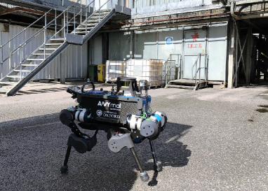
Figure 1: Experiments were conducted using an ANYbotics ANYmal quadruped [5] in outdoor environments, including the Oil Rig training facility shown above. The ANYmal robot has 12 actuated degrees of freedom, an IMU, dual forward-facing RealSense D435 cameras and a Velodyne VLP-16 LIDAR. Video: https://youtu.be/p8o7mJPy4_w.

To overcome this limitation, some previous works have incorporated exteroceptive inputs (cameras and LIDAR) into filtering estimators in a loosely coupled fashion. This has been successfully demonstrated on legged machines operating in field experiments [6, 7].

However, because these filters marginalize all previous states of the robot, it is not possible to fully exploit a (recent) history of measurements, as smoothing methods can.

Research into smoothing approaches applied to Visual-Inertial Navigation Systems (VINS) is now well established in the Micro-Aerial-Vehicle (MAV) community. On a MAV this approach has been successful due to careful time synchronization of the IMU and cameras, smooth vehicle motion, and also the absence of the challenges of articulated legged machines.

A recent work by Hartley et al. [8] demonstrated that a VINS approach could be adapted to legged robots — in their case, a biped. Their initial results were promising, but only tested in a controlled scenario. Additionally, vision was integrated as relative pose constraints, rather than incorporating the feature residuals directly into the optimization.

Contribution

This paper aims to progress the deployment of state estimation smoothing methods in realistic application scenarios. Compared to previous research, we present the following contributions:

• We present the first state estimation method based on factor graphs that tightly integrates visual features directly into the cost function (rather than adding a pose constraint from a separate visual inertial module), together with preintegrated inertial factors and relative pose constraints from the kinematics. We will refer to our proposed method as VILENS (Visual Inertial LEgged Navigation System);

• We demonstrate the performance and robustness of our method with extensive experiments on two field scenarios. Challenges included motion blur, dynamic scene occludants, textureless and reflective scenes, and locomotion on uneven, muddy and slippery terrain;

• We demonstrate that a low-cost consumer-grade depth camera, the RealSense D435, is sufficient to significantly improve the state estimate in these conditions.

The remainder of the article is presented as follows: in Section II we describe the previous research in the field; the theoretical background of the algorithm is described in Sections III and IV. Section V outlines the details of our implementation. The experimental results and their discussion are shown in Sections VI and VII. Finally, Section VIII concludes the article.

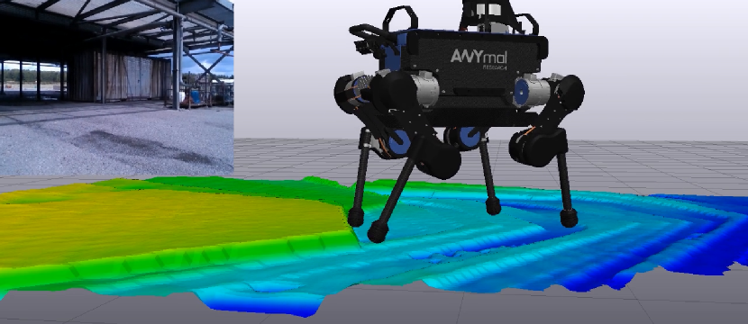
Figure 2: An elevation map created by the GridMap package [9] while walking over flat terrain shows discrete ridges due to position drift in the current kinematic state estimator. This makes dynamic locomotion and footstep planning much more challenging.

II Related Work

Multi-sensor fusion for mobile robot state estimation has been widely described in the literature [10]. Here, we limit our discussion to filtering and smoothing approaches with particular focus on dynamic legged robots.

II-A Filtering Approaches

After the spread of filtering methods for proprioceptive state estimation [1], there has been interest in including exteroceptive data, particularly Visual Odometry (VO).

Ma et al. [6] presented a method based on an Extended Kalman Filter (EKF) with an error state formulation developed for the Boston Dynamics LS3. The system was primarily driven by inertial predictions with VO updates: a modular sensor head performs the fusion of a very high quality tactical grade IMU with two hardware synchronized stereo cameras. The leg odometry (fused with an additional navigation grade IMU in the body) was used only in case of VO failure. Their extensive evaluation (over several $\mathrm{km}\text{/}$) achieved $1\text{\,}\mathrm{\char 37\relax}\text{/}$ error per distance traveled.

Nobili et al. [7] recently presented a state estimator for the HyQ quadruped robot which used an EKF to combine inertial, kinematic, visual, and LIDAR measurements. In contrast to [6], the EKF was driven by an inertial process model with the primary corrections coming from leg odometry (synchronized in EtherCAT) at the nominal control rate ($1\text{\,}\mathrm{kHz}\text{/}$). The VO updates and an ICP-based matching algorithm were run on a separate computer at lower frequency and integrated into the estimator when available. This allowed the use of the estimator inside the control loop and has been recently demonstrated in dynamic motions with local mapping [11].

II-B Smoothing Approaches

There has been a significant body of work on visual inertial navigation, especially for use with MAVs. A recent benchmark paper [12] evaluated a number of state-of-the-art methods on the EuRoC dataset [13]. The maturity of the field was highlighted by the fact that many algorithms achieved an average Relative Position Error (RPE) of less than $20\text{\,}\mathrm{cm}\text{/}$ per $35\text{\,}\mathrm{m}\text{/}$ traveled. The authors concluded that the best performing algorithms were OKVIS [14], ROVIO [15], and VINS-Mono [16]. All of these algorithms perform windowed optimization to achieve the most accurate state estimate while bounding computation time. An exception was SVO+GTSAM [17] which loosely coupled the SVO visual odometry algorithm with IMU data using iSAM2 as the smoothing back-end [18].

The methods were, however, typically designed assuming that the IMU and cameras were synchronized in hardware, and that the vehicle motions were smooth. They are difficult to implement on legged platforms due to their hardware complexity and the high vibrations caused by locomotion.

As mentioned above, the first approach to use smoothing/optimization on legged robots was the work of Hartley et al. [8] which presented a fusion of kinematic, inertial, and visual information, again using iSAM2 as the smoothing back-end. They presented a mathematical framework to model contact points as landmarks in the environment, similar to [1]. Their system incorporated contact information from only a single contact point at a time, and directly integrates (as pose constraints) the relative motion estimate of the SVO2 [19] algorithm. The approach was tested using inertial and visual input from a MultiSense S7 sensor (which was hardware synchronized) mounted on a Cassie biped (from Agility Robotics). A short indoor experiment of $60\text{\,}\mathrm{s}\text{/}$ showed that adding vision into the optimization reduced the relative position error.

Our approach aims to combine best practice from the mature field of VINS – including windowed optimization and tight integration of visual features – with legged odometry to provide robust state estimation for legged robots. In Section VI we show our system outperforming both kinematic-inertial and visual-inertial approaches in large-scale outdoor urban and industrial experiments.

III Problem Statement

We wish to track the linear position and velocity of a 12 Degrees of Freedom (DoF) legged robot equipped with an industrial grade MEMS IMU, an RGB/IR camera, joint encoders and torque sensors. The sensor specifications are detailed in Table I.

TABLE I: Sensor specifications

Sensor	Model	$\mathrm{Hz}\text{/}$	Specs
IMU	Xsens MTi-100	400	Init Bias: $0.2\text{\,}\mathrm{\SIUnitSymbolDegree}\text{/}\mathrm{s}$ $~{}|~{}$ $5\text{\,}\mathrm{mg}\text{/}$
			Bias Stab: $10\text{\,}\mathrm{\SIUnitSymbolDegree}\text{/}\mathrm{h}$ $~{}|~{}$ $15\text{\,}\mathrm{mg}\text{/}$
Camera	RealSense D435	30	Keble College Dataset:
			Resolution: $848\times 480$ px
			FoV: $91.2\text{\times}65.5\text{\,}\mathrm{\SIUnitSymbolDegree}\text{/}$
			Imager: IR global shutter
			Oil Rig Dataset:
			Resolution: $640\times 480$ px
			FoV: $69.4\text{\times}42.5\text{\,}\mathrm{\SIUnitSymbolDegree}\text{/}$
			Imager: RGB rolling shutter
Encoder	ANYdrive	400	Resolution: $<0.025\text{\,}\mathrm{\SIUnitSymbolDegree}\text{/}$
Torque	ANYdrive	400	Resolution: $<0.1\text{\,}\mathrm{N}\text{\,}\mathrm{m}\text{/}$

In Fig. 3 we provide a schematic of the reference frames involved. The pose of the robot’s base $\mathtt{{B}}$ expressed in the fixed-world, inertial frame $\mathtt{W}$ is defined as:

$$\mathbf{T}_{\mathtt{W}\mathtt{{B}}}=\begin{bmatrix}\mathbf{R}_{\mathtt{{W}}\mathtt{{B}}}&\tensor[_{\mathtt{{W}}}]{\mathbf{p}}{{}_{\mathtt{{W}}\mathtt{{B}}}}\\ \boldsymbol{0}&1\end{bmatrix}\in\mathrm{SE}(3)$$

The IMU and camera sensing frames are $\mathtt{I}$ and $\mathtt{C}$, respectively. The relative transformations between $\mathtt{{B}}$, $\mathtt{I}$ and $\mathtt{C}$ are assumed to be known from CAD design. The location of a foot in base coordinates is expressed as $\tensor[_{\mathtt{{B}}}]{\mathbf{p}}{{}_{\mathtt{{B}}\mathtt{K}}}$.

III-A State Definition

Borrowing the notation from [17], we define the state of the system at time $t_{i}$ as:

$$\boldsymbol{x}_{i}\triangleq[\mathbf{R}_{i},\mathbf{p}_{i},\mathbf{v}_{i},\mathbf{b}_{i}]$$ (1)

where the couple $(\mathbf{R}_{i},\mathbf{p}_{i})$ expresses the robot pose and $\mathbf{v}_{i}\in\mathbb{R}^{3}$ is the robot linear velocity. As is common in this field, the stack of gyro and accelerometer IMU biases $\mathbf{b}_{i}=[\mathbf{b}^{\omega}_{i}\;\;\mathbf{b}^{a}_{i}]\in\mathbb{R}^{6}$ replaces the angular velocity, which is directly measured by the IMU.

Figure 3: Reference frames conventions. The world frame $\mathtt{W}$ is fixed to earth, while the base frame $\mathtt{{B}}$, the camera’s optical frame $\mathtt{C}$, and the IMU frame, $\mathtt{I}$ are rigidly attached to the robot’s chassis. When a foot touches the ground (e.g., the Right Front, RF), a contact frame $\mathtt{K}$ (perpendicular to the ground and parallel to $\mathtt{W}$’s $y$-axis) is defined. The projection of a landmark point $\mathbf{m}$ onto the image plane is $\pi(\mathbf{m})$.

Let $\mathsf{K}_{k}$ be the set of camera keyframe indices up to time $t_{k}\in\mathbb{R}$. We assume that for each keyframe image ${\cal C}_{i}$ (with $i\in\mathsf{K_{k}}$) a number of landmark points $\tensor[_{\mathtt{{W}}}]{\mathbf{m}}{{}_{j}}$ are visible, where $j\in\mathsf{M}_{i}\subseteq\mathsf{M}$; $\mathsf{M}_{i}$ indicates the set of landmark indices visible from keyframe ${\cal C}_{i}$ out of the full set of landmarks, $\mathsf{M}$. We then define the objective of our estimation problem $\mathcal{X}_{k}$ as the history of robot states and landmarks detected up to $t_{k}$:

$$\mathcal{X}_{k}\triangleq\bigcup_{\forall i\in\mathsf{K}_{k}}\left[\{\boldsymbol{x}_{i}\}_{,}\bigcup_{\forall j\in\mathsf{M}_{i}}\{\mathbf{m}_{j}\}\right]$$ (2)

III-B Measurements

The input measurements consist of camera images, IMU readings, and joint sensing (position, velocity and torque). The measurements are not assumed to be synchronized. However, we assume they have a common time frame. The IMU and joint states have the same frequency (see Fig. 4). For each pair of consecutive keyframe indices $\Delta i=i-1,i\in\mathsf{K}_{k}$ we define $\mathsf{I}_{\Delta i}$ as the set of IMU measurements indices such that $\forall~{}m\in\mathsf{I}_{\Delta i}$ we have $t_{i-1}\leq t_{m}<t_{i}$. We then indicate with ${\cal I}_{\Delta i}=\bigcup_{\forall j\in\mathsf{I}_{\Delta i}}(\boldsymbol{\omega}_{j},{\mathbf{a}}_{j})$ all angular velocity and proper acceleration measurements collected between time $t_{i-1}$ and $t_{i}$. Analogous definitions apply to joint states ${\cal Q}_{\Delta i}=\bigcup_{\forall j\in\mathsf{Q}_{\Delta i}}(\mathbf{q}_{j},\dot{\mathbf{q}}_{j},\boldsymbol{\tau}_{j})$, which include all joint positions, velocities and torques collected between time $t_{i-1}$ and $t_{i}$. Strategies to account for synchronization issues are discussed in Section V-A.

Finally, we then let $\mathcal{Z}_{k}$ denote the set of all measurements up to time $t_{k}$:

$$\mathcal{Z}_{k}\triangleq\bigcup_{\forall i\in\mathsf{K}_{k}}\left\{{\cal I}_{\Delta i},{\cal C}_{i},{\cal Q}_{\Delta i}\right\}$$ (3)

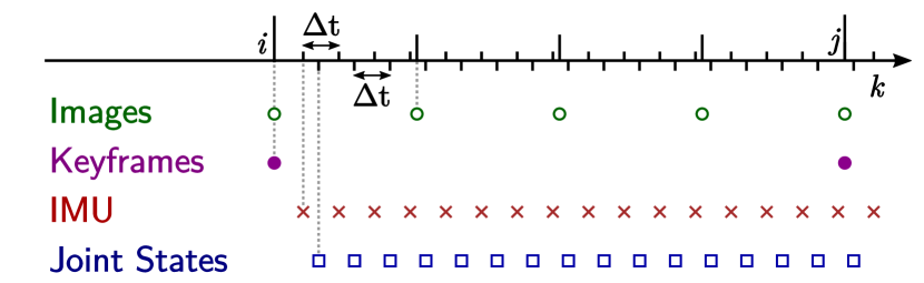
Figure 4: The sensors inputs are images, IMU measurements, and joint states, which are in general unsynchronized with each other.

III-C Maximum-A-Posteriori Estimation

The aim of the factor graph framework is to maximize the posterior the history of states and landmarks $\mathcal{X}_{k}$, given the history of measurements $\mathcal{Z}_{k}$:

$$\mathcal{X}^{*}_{k}=\operatorname*{arg\,max}_{\mathcal{X}_{k}}p(\mathcal{X}_{k}|\mathcal{Z}_{k})\propto p(\mathcal{X}_{0})p(\mathcal{Z}_{k}|\mathcal{X}_{k})$$ (4)

Where the last member of (4) is the likelihood function, which is proportional to the posterior and therefore can be used as a cost function. If the measurements are conditionally independent and corrupted by zero mean Gaussian noise, then (4) is equivalent to a least squares problem of the form:

$$\mathcal{X}^{*}=\operatorname*{arg\,min}_{\mathcal{X}_{k}}\sum_{{\cal T}}\sum_{\forall i\in\mathsf{K}_{k}}\|\mathbf{r}_{{\cal T}_{i}}\|^{2}_{\Sigma_{{\cal T}_{i}}}$$ (5)

where $\mathbf{r}_{{\cal T}_{i}}$ is the residual of the error between the predicted and measured value of type ${\cal T}$ (e.g., IMU ${\cal I}$) at keyframe index $i\in\mathsf{K}_{k}$. The quadratic cost of each residual is weighted by the corresponding covariance $\Sigma_{{\cal T}_{i}}$.

From (2) and (3) the optimization becomes the following:

$$\mathcal{X}^{*}=\operatorname*{arg\,min}_{\mathcal{X}}\sum_{j\in M}\|\mathbf{r}_{\mathbf{m}_{j,0}}\|^{2}_{\Sigma_{\mathbf{m}_{j,0}}}+\sum_{i\in\mathsf{K}_{k}}\|\mathbf{r}_{{\cal I}_{\Delta i}}\|^{2}_{\Sigma_{{\cal I}_{\Delta i}}}+\\ +\|\mathbf{r}_{0}\|^{2}_{\Sigma_{0}}+\sum_{i\in\mathsf{K}_{k}}\sum_{j\in\mathsf{M}_{i}}\|\mathbf{r}_{\mathbf{m}_{j}}\|^{2}_{\Sigma_{\mathbf{m}_{j}}}+\sum_{i\in\mathsf{K}_{k}}\|\mathbf{r}_{{\cal Q}_{\Delta i}}\|^{2}_{\Sigma_{{\cal Q}_{\Delta i}}}$$ (6)

where the residuals are from: landmark prior, IMU, state prior, camera and leg odometry factors, respectively. These factors will be used to create the factor graph structure shown in Fig. 5. In the next section we define each residual of (6).

IV Factor Definitions

Figure 5: The factor graph consists of state and landmark nodes linked by prior, visual, inertial, and leg odometry factors.

IV-A Prior Factors

Since this is an odometry system, prior factors are required during initialization to anchor the unobservable modes (i.e., position and yaw) to a fixed reference frame. The residual is defined as the error between the estimated state $\boldsymbol{x}_{0}$ and the prior $\boldsymbol{x}_{p_{0}}$:

$$\mathbf{r}_{0}(\boldsymbol{x}_{0},\mathcal{Z})=\left(\begin{array}[]{c}\Phi(\mathbf{T}_{0}^{-1}\mathbf{T}_{p_{0}})\\ \mathbf{v}_{0}-\mathbf{v}_{p_{0}}\\ \mathbf{b}_{0}^{a}-\mathbf{b}_{p_{0}}^{a}\\ \mathbf{b}_{0}^{\omega}-\mathbf{b}_{p_{0}}^{\omega}\end{array}\right)$$ (7)

where $\Phi:\mathrm{SE}(3)\mapsto\mathbb{R}^{6}$ is the lifting operator [17]. The prior state of the system is determined by IMU initialization, assuming the robot is stationary.

IV-B Visual Odometry Factors

The visual odometry residual consists of two components. The first is the difference between the measured landmark pixel location, $(u_{i,j},\;v_{i,j})$, and the re-projection of the estimated landmark location into image coordinates, $(\pi_{u},\pi_{v})$ using the standard radial-tangential distortion model. The residual is defined as:

$$\mathbf{r}_{\mathbf{m}_{j}}=\left(\begin{array}[]{c}\pi_{u}(\mathbf{R}_{i},\mathbf{p}_{i},\mathbf{m}_{j})-u_{i,j}\\ \pi_{v}(\mathbf{R}_{i},\mathbf{p}_{i},\mathbf{m}_{j})-v_{i,j}\end{array}\right)$$ (8)

The second is the error between the prior on the landmark location $\mathbf{m}_{j,0}$ and the estimated landmark location $\mathbf{m}_{j}$:

$$\mathbf{r}_{\mathbf{m}_{j,0}}=\mathbf{m}_{j}-\mathbf{m}_{j,0}$$ (9)

Legged robots typically move dynamically with velocities parallel to the optical axis of the camera. This motion can lead to underconstrained landmark positions. To this end, a landmark prior is generated online through an initial triangulation procedure (see Section V). The covariance, $\Sigma_{\mathbf{m}_{i,j}}$, is determined by the typical feature tracking accuracy (in our case, we use 1 pixel).

IV-C Preintegrated IMU Factors

We use the IMU preintegration algorithm described by Forster et al. [17]. This approach preintegrates the IMU measurements between nodes in the factor graph to provide high frequency state updates between optimization steps. The preintegrated IMU measurements are then used to create a new IMU factor between two consecutive keyframes. This will use an error term of the form:

$$\mathbf{r}_{{\cal I}_{\Delta i}}=\left[\mathbf{r}^{\mathsf{T}}_{\Delta\mathbf{R}_{\Delta i}},\mathbf{r}^{\mathsf{T}}_{\Delta\mathbf{p}_{\Delta i}},\mathbf{r}^{\mathsf{T}}_{\Delta\mathbf{v}_{\Delta i}},\mathbf{r}^{\mathsf{T}}_{\Delta\mathbf{b}_{\Delta i}}\right]$$ (10)

where ${\cal I}_{\Delta i}$ are the IMU measurements between times $i-1$ and $i$. The individual elements of the residual are defined as:

$$\mathbf{r}_{\Delta\mathbf{R}_{\Delta i}} = \log\left(\Delta\tilde{\mathbf{R}}_{\Delta i}(b^{g}_{i-1})\right)\mathbf{R}^{T}_{i-1}\mathbf{R}_{i}$$ (11)

$$\mathbf{r}_{\Delta\mathbf{p}_{\Delta i}} = \mathbf{R}^{T}_{i-1}\left(\mathbf{p}_{i}-\mathbf{p}_{i-1}-\mathbf{v}_{i-1}\Delta t_{\Delta i}-\frac{1}{2}\mathbf{g}\Delta t_{\Delta i}^{2}\right)$$ (12)

$$-\Delta\tilde{\mathbf{p}}_{\Delta i}(b^{g}_{i-1},b^{a}_{i-1})$$

$$\mathbf{r}_{\Delta\mathbf{v}_{\Delta i}} = \mathbf{R}^{T}_{i-1}\left(\mathbf{v}_{i}-\mathbf{v}_{i-1}-\mathbf{g}\Delta t_{\Delta i}\right)$$ (13)

$$-\Delta\tilde{\mathbf{v}}_{\Delta i}(b^{g}_{i-1},b^{a}_{i-1})$$

$$\mathbf{r}_{\Delta\mathbf{b}_{\Delta i}} = \mathbf{b}_{i}-\mathbf{b}_{i-1}$$ (14)

where $\Delta\tilde{\mathbf{R}}_{\Delta i},\Delta\tilde{\mathbf{p}}_{\Delta i},\Delta\tilde{\mathbf{v}}_{\Delta i}$ are the preintegrated IMU measurements defined in [17]. The covariance, $\Sigma_{{\cal I}_{\Delta i}}$, is based on an offline Allan Variance analysis.

IV-D Leg Odometry Factors

Leg Odometry (LO) estimates the incremental motion of a walking robot given its kinematic sensing and the perceived contacts between the robot’s feet and the ground. The main assumption behind LO measurements is that the absolute velocity of a contact point is zero. This condition is met when the Ground Reaction Force (GRF) at a contact point is inside a hypothetical friction cone. Torques at contact points are neglected as quadruped robots’ feet are idealized as points.

Since the GRF, the terrain inclination, and the coefficient of static friction are typically unknown, an appropriate fusion of the dynamic model, kinematics, and IMU is required. In this work, we rely on the state estimator provided by ANYbotics, the Two-State Implicit Filter (TSIF) [3]. We use the relative robot motion estimated by the TSIF to formulate relative pose factors so as to further constrain the robot’s motion estimate from the factor graph.

Given two keyframes at times $t_{i-1}$ and $t_{i}$, the corresponding pose estimates $\widetilde{\mathbf{T}}_{i-1},\;\widetilde{\mathbf{T}}_{i}$ are computed via linear/slerp interpolation from the filter history and used to produce the relative pose constraint:

$$\mathbf{r}_{{\cal Q}_{\Delta i}}=\Phi\left((\mathbf{T}_{i-1}^{-1}\mathbf{T}_{i})^{-1}\widetilde{\mathbf{T}}_{i-1}^{-1}\widetilde{\mathbf{T}}_{i}\right)$$ (15)

where the covariance $\Sigma_{{\cal Q}_{\Delta i}}$ is provided by the filter, and $\Phi$ is the lifting operator defined in [17].

IV-E Zero Velocity Update Factors

To limit drift and factor graph growth when the robot is stationary, we detect zero velocity motion from camera frames by calculating the average feature motion:

$$\overline{\Delta x}=\frac{\sum_{i=k-N}^{k}\left(\sqrt{(u_{i}-u_{i-1})^{2}+(v_{i}-v_{i-1})^{2}}\right)}{N+1}$$ (16)

If $\overline{\Delta x}$ is below a certain threshold $\beta=0.5$ pixels over $N=10$ successive frames, we stop adding image landmark measurements to the graph and simply add a zero relative pose factor to the graph of the same form as (15). The thresholds were tuned by calculating $\overline{\Delta x}$ when the camera was stationary. These factors reduce computation when the robot is stationary and can reduce overall drift by up to 20%.

V Implementation

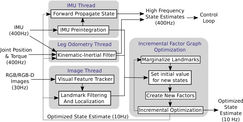
Figure 6: The proposed state estimation architecture consists of measurement handlers which process the sensor input and the current state from the optimizer to create the factors. These factors are then smoothed using iSAM2 for incremental factor graph optimization.

The factor graph optimization was implemented using the iSAM2 incremental optimization library [18]. The structure of the system is shown in Fig. 6. The algorithm consists of a series of measurement handlers running in separate threads that process the different sensor inputs. When a new node is created (e.g., when an image measurement is received) each of the measurement handlers adds new factors to the graph. The output of the factor graph optimization is then fed back to the measurement handlers.

V-A Synchronization

Given two consecutive keyframe indices $i-1,i\in\mathsf{K}_{k}$, preintegrating all IMU measurements between times $t_{i-1}$ and $t_{i}$ would result in an incorrect motion estimation as the IMU measurement timestamps may not be aligned with the image frames (see Fig. 7). To avoid this, we correct the $\Delta t$ of the IMU measurements directly before and after the camera image timestamp $t_{i}$:

$$\Delta t_{i-1} = t_{\textsc{imu}}+\Delta t_{\textsc{imu}}-t_{i}$$ (17)

$$\Delta t_{i} = t_{i}-t_{\textsc{imu}}$$ (18)

where we assume constant acceleration and angular velocity between IMU measurements.

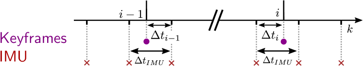
Figure 7: We consider and account for camera/IMU asynchronousity so as to improve the accuracy of the IMU factors.

V-B Visual Feature Tracking

A core component of the VILENS system is the tight integration of visual features into the optimization. It can provide lower drift state estimates by tracking and optimizing the robot state and landmark positions over many observations. Our visual feature tracking method is based upon the robust pixel-based tracking approaches used in ROVIO [20] and VINS-Mono [16].

Visual features are first detected using the Harris Corner Detector and then tracked through successive images using the Kanade-Lucas-Tomasi feature tracker. This method provides sub-pixel accuracy and is well-suited to the constrained but jerky motions typical of a legged robot. After the tracking, outliers are rejected using RANSAC with a fundamental matrix model similar to [16]. New features are then detected in the image to maintain a minimum number of tracked features. These new features are constrained to be a minimum distance (in image space) from existing features, to ensure an even distribution of features across the image.

To limit the graph growth, we estimate the location of a feature in the world frame only after it has been observed more than $N_{\text{obs}}=30$ times. When depth is available, it is used for the initial landmark location estimate. When only monocular data are available, we triangulate the landmark location $\mathbf{m}_{j,0}$ using the last $N_{\text{obs}}$ frames with the Direct Linear Transformation (DLT) algorithm from [21]. If the landmark is successfully triangulated with a depth smaller than $d_{\text{max}}=$50\text{\,}\mathrm{m}\text{/}$$ then this and successive measurements of the same landmark are added to the graph.

V-C Marginalization

An important consideration in a legged robot system is latency, and without marginalization, the time taken by iSAM2 optimization increases over time [18]. This becomes an important consideration when operating the robot for extended periods of time.

We marginalize states older than a threshold (typically, $10\text{\,}\mathrm{s}\text{/}$) and landmarks which are no longer observed, whilst keeping a minimum number of nodes in the factor graph. These marginalized states and landmarks are replaced with a simple linear Gaussian factor based on the current linearization point of the node. This Gaussian factor has the same form as the residual defined in (7).

VI Experimental Results

In this section, we present the experimental evaluation of the proposed algorithm on three different datasets: EuRoC, Keble College and Oil Rig. The first dataset is a purely VINS dataset collected on a MAV. The other two datasets were collected using our ANYmal robot in different outdoor environments: a college campus and an industrial oil rig firefighter training facility.

VI-A EuRoC Dataset

To demonstrate that our approach builds upon a stand-alone VINS system, we evaluated it on a portion of the EuRoC benchmark dataset [13] and compared it to several state-of-the-art VINS algorithms including OKVIS [14], ROVIO [20], and VINS-Mono [16]. The estimated trajectory from the EuRoC V2_01 dataset is shown in Fig. 8.

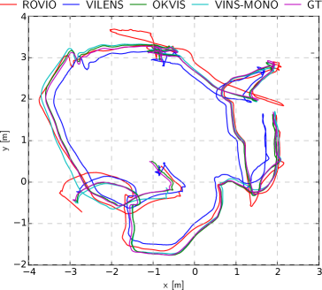
Figure 8: Performance comparison between our baseline VILENS system (blue), ROVIO (red), OKVIS (green), and VINS-Mono (cyan) compared to VICON ground truth for EuRoC V2_01 dataset.

In brief, we found that our core system can achieve comparable performance to these VINS algorithms. This demonstrates that the estimator can function without leg odometry information, which is important when that modality becomes unreliable (e.g., on slippery or soft ground).

VI-B Outdoor Datasets Experimental Setup

The outdoor experiments were conducted using the 12-DoF ANYmal quadruped [5] (Fig. 1).

The measurements from the motors (i.e., joint states) were synchronized via EtherCAT, while the other sensors were synchronized by Network Time Protocol (NTP). The sensor configurations used for the two datasets are specified in Table I.

To generate ground truth, we collected a dense gravity-aligned prior map of the site using the Leica BLK-360 3D laser scanner. Afterwards, we performed ICP localization (using the AICP algorithm [22]) against the prior map using data from ANYmal’s Velodyne VLP-16 LIDAR. Both map and LIDAR sensor were used as the ground truth only. This provided a ground truth trajectory with approximately $5\text{\,}\mathrm{cm}\text{/}$ accuracy, but only at $2\text{\,}\mathrm{Hz}\text{/}$.

VI-C Keble College Dataset

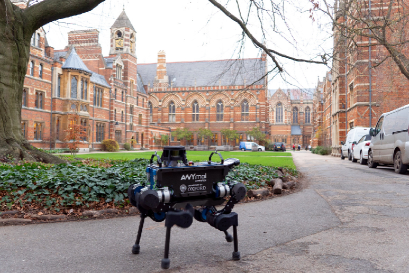
Figure 9: The Keble College dataset involved the ANYmal trotting around an open urban environment.

The first outdoor dataset was collected in a urban environment at Keble College, Oxford, UK. The dataset consists of the robot trotting on a concrete path around a $28\text{\times}60\text{\,}\mathrm{m}\text{/}$ open lawn surrounded by a residential building (Fig. 9). The main challenges were vegetation moving in the wind, long distances to visual features ($>10\text{\,}\mathrm{m}\text{/}$), and limited angular motion, which made feature triangulation difficult.

We ran four trials each approximately $22\text{\,}\mathrm{m}\text{/}$ in length and evaluated the mean and standard deviation of the Relative Position Error (RPE) over a $10\text{\,}\mathrm{m}\text{/}$ distance (see Table II). Compared to the kinematic-inertial estimator, our algorithm reduces the RPE by $15\text{\,}\mathrm{\char 37\relax}\text{/}$ to $55\text{\,}\mathrm{\char 37\relax}\text{/}$ and yaw error by $42\text{\,}\mathrm{\char 37\relax}\text{/}$ to $85\text{\,}\mathrm{\char 37\relax}\text{/}$, as visual features tracked over many frames constrain pose drift.

TABLE II: Mean (and standard deviation) performance on the Keble College and Oil Rig datasets.

	RPE $\boldsymbol{\mu(\sigma)}$ [$\mathrm{m}\text{/}$]		Yaw Error $\boldsymbol{\mu(\sigma)}$ [$\deg$]
Dataset	TSIF [3]	VILENS	TSIF [3]	VILENS
Keble 1	0.53 (0.21)	0.30 (0.12)	6.64 (2.23)	0.99 (0.80)
Keble 2	0.51 (0.10)	0.23 (0.10)	5.72 (0.94)	1.47 (1.07)
Keble 3	0.67 (0.10)	0.52 (0.15)	6.68 (0.80)	3.86 (1.90)
Keble 4	0.47 (0.11)	0.40 (0.10)	3.32 (1.15)	1.13 (1.46)
Oil Rig	0.44 (0.37)	0.41 (0.18)	4.89 (3.38)	3.68 (4.10)

VI-D Oil Rig Dataset

A second outdoor dataset was collected at an industrial firefighter training facility in Moreton-In-Marsh, UK (Fig. 1). The facility closely matches the locations where ANYmal is likely to be deployed in future.

This $110\text{\,}\mathrm{m}\text{/}$ ($22\text{\,}\mathrm{min}\text{/}$) long dataset involves the ANYmal robot trotting through the facility, climbing over a slab, and walking up a staircase into a smoke-blackened room. Challenging situations include: featureless areas, stationary periods with intermittent motion, dynamic obstacles occluding large portions of the image, non-flat terrain traversal, and foot slip caused by a combination of mud, oil, and water on the ground (Fig. 11).

Figure 10 shows the estimated trajectory from VILENS, compared to TSIF [3] and ground truth. The Absolute Translation Error (ATE) for VILENS is $76\text{\,}\mathrm{\char 37\relax}\text{/}$ lower compared to the TSIF ($1.65\text{\,}\mathrm{m}\text{/}$ and $6.88\text{\,}\mathrm{m}\text{/}$, respectively).

Looking at the relative performance over $10\text{\,}\mathrm{m}\text{/}$, the error reduction is $7\text{\,}\mathrm{\char 37\relax}\text{/}$ for RPE and $25\text{\,}\mathrm{\char 37\relax}\text{/}$ for yaw (Table III). This suggests that the Oil Rig dataset is more challenging than Keble, since the accuracy at small scale is closer to the TSIF (see Section VII).

Note that performance evaluation against the VINS algorithms mentioned in Section VI-A was not possible because they either failed to initialize due to the lack of motion or diverged after a short period. This is also confirmed in Table III, where we evaluated the performance of VILENS as standalone VINS system against TSIF and full VILENS. Without Leg Odometry factors, VILENS fails for all the datasets except the first $70\text{\,}\mathrm{s}\text{/}$ of Keble 1 and Oil Rig, where it performs worse or same.

TABLE III: Mean (and standard deviation) performance of TSIF, VILENS as VINS system, and VILENS before VINS failure ($\sim 70\text{\,}\mathrm{s}\text{/}$)

	RPE $\boldsymbol{\mu(\sigma)}$ [$\mathrm{m}\text{/}$]			Yaw Error $\boldsymbol{\mu(\sigma)}$ [$\deg$]
Dataset	TSIF	VINS	VILENS	TSIF	VINS	VILENS
Keble 1	0.30	0.36	0.25	4.28	0.74	0.75
	(0.06)	(0.12)	(0.13)	(1.07)	(0.61)	(0.56)
Oil Rig	1.09	5.33	0.34	10.38	5.03	1.21
	(0.09)	(0.53)	(0.12)	(0.75)	(3.21)	(0.90)

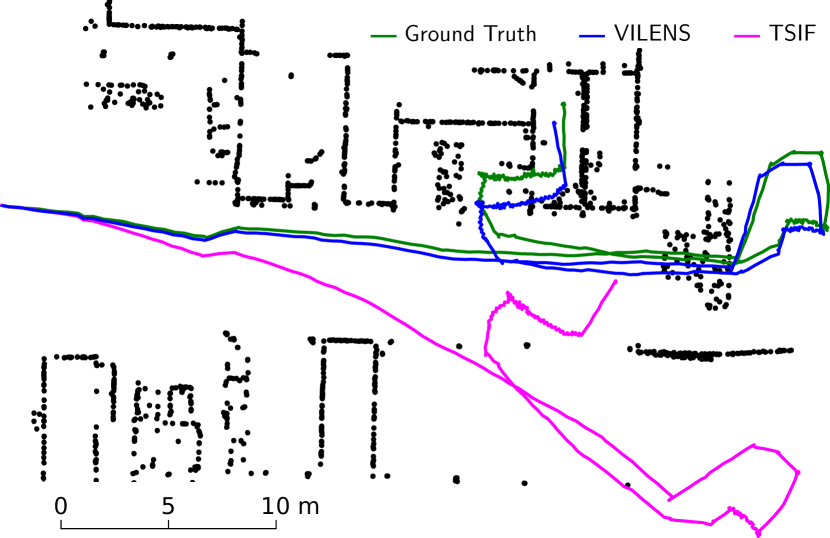
Figure 10: Top view of the estimated trajectories of VILENS (blue), TSIF (magenta), and ground truth (green) on the Oil Rig Dataset. The map is not used in the algorithm and is shown for illustrative purposes only.

VI-E Timing

A summary of the key computation times in the proposed algorithm are shown in Table IV. Since the kinematic-inertial filter, the image processing, and the optimization are run in separate threads, the system is capable of outputting a high-frequency kinematic-inertial state estimate (for control purposes) at $400\text{\,}\mathrm{Hz}\text{/}$, and an optimized estimate incorporating visual features at approximately $10\text{\,}\mathrm{Hz}\text{/}$.

TABLE IV: Mean (and standard deviation) processing time for components of the VILENS system, on the Oil Rig dataset.

Thread	Module	$\boldsymbol{\mu(\sigma)}$ [$\mathrm{ms}\text{/}$]
Optimization	Factor Creation	10.80 (4.50)
	Optimization	10.05 (7.69)
	Marginalization	0.82 (0.97)
	Total	21.67 (13.12)
Image Proc	Image Equalization	0.87 (0.51)
	Feature Tracking	2.04 (0.98)
	Outlier Rejection	1.74 (1.87)
	Feature Detection	5.33 (0.91)
	Total	9.99 (4.27)

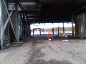
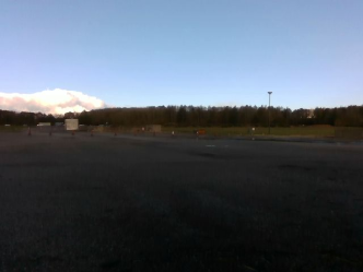
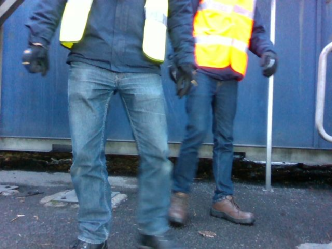
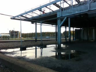
Figure 11: Notable situations within the Oil Rig dataset. Top-Left: VILENS outperforms TSIF where there are many visual features. Top-Right: VILENS and TSIF perform similarly where there is no structure in front of the robot. Bottom: Moving objects and reflections are robustly handled by VILENS.

VII Discussion

In the previous section, we have demonstrated that VILENS outperforms kinematic-inertial and visual-inertial methods for all the datasets. However, from Table II we can see that the gap between VILENS and TSIF is not uniform across the datasets.

An in-depth analysis of performance was limited by the accuracy and frequency of our LIDAR ground truth. Nonetheless, we see that the feature quality has an influence of the drift rate over small scales.

In Fig. 12 we compare the drift rate of VILENS and TSIF over different distance scales for the Keble College and the Oil Rig datasets. The latter experiment is more challenging from the perspective of exteroception and as a result the scale at which VILENS starts to outperform TSIF is larger. This is due to the tracking of poor quality features in the conditions highlighted in Fig. 11.

In future work, we are motivated to improve performance in these challenging scenarios by exploring the use of redundant or wider field-of-view cameras as well as different methods of incorporating the kinematics directly into the factor graph. Additionally, as part of an ongoing project, we intend to test performance in soft and compliant surface materials such as sand, mud and gravel where we envisage the visual part of the estimator predominating during sinking, sliding and slipping.

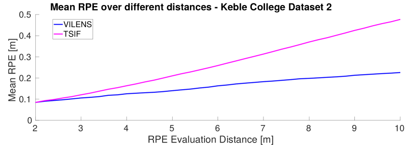
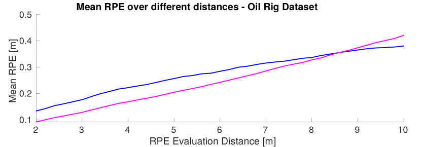
Figure 12: Mean RPE for VILENS and TSIF at different distance scales. Top: Keble College Dataset. Bottom: Oil Rig Dataset. The Oil Rig dataset is more challenging and therefore VILENS outperforms TSIF at larger distance ($~{}8.5\text{\,}\mathrm{m}\text{/}$) than for Keble.

VIII Conclusion

In this paper, we have presented VILENS (Visual Inertial LEgged Navigation System), a robust state estimation method for legged robots based on factor graphs, which incorporates kinematic, inertial and visual information. This method outperforms the robot’s kinematic-inertial estimator and robustly estimates the robot trajectory in challenging scenarios, including textureless areas, moving occludants, reflections and slippery ground. Under the same conditions, current state-of-the-art visual-inertial algorithms diverge rapidly.

References

- [1] M. Bloesch, M. Hutter, M. A. Hoepflinger, S. Leutenegger, C. Gehring, C. David Remy, and R. Siegwart, “State Estimation for Legged Robots - Consistent Fusion of Leg Kinematics and IMU,” in Robotics: Science and Systems VIII, 2012.
- [2] M. Camurri, M. Fallon, S. Bazeille, A. Radulescu, V. Barasuol, D. G. Caldwell, and C. Semini, “Probabilistic Contact Estimation and Impact Detection for State Estimation of Quadruped Robots,” IEEE Robotics and Automation Letters, vol. 2, no. 2, pp. 1023–1030, 2017.
- [3] M. Bloesch, M. Burri, H. Sommer, R. Siegwart, and M. Hutter, “The Two-State Implicit Filter - Recursive Estimation for Mobile Robots,” IEEE Robotics and Automation Letters, vol. 3, no. 1, pp. 573–580, 2017.
- [4] P. Fankhauser, M. Bjelonic, C. Dario Bellicoso, T. Miki, and M. Hutter, “Robust Rough-Terrain Locomotion with a Quadrupedal Robot,” in IEEE International Conference on Robotics and Automation, 2018.
- [5] M. Hutter, C. Gehring, D. Jud, A. Lauber, C. D. Bellicoso, V. Tsounis, J. Hwangbo, K. Bodie, P. Fankhauser, M. Bloesch, R. Diethelm, S. Bachmann, A. Melzer, and M. A. Hoepflinger, “ANYmal - A Highly Mobile and Dynamic Quadrupedal Robot,” in IEEE International Conference on Intelligent Robots and Systems, 2016, pp. 38–44.
- [6] J. Ma, M. Bajracharya, S. Susca, L. Matthies, and M. Malchano, “Real-time pose estimation of a dynamic quadruped in GPS-denied environments for 24-hour operation,” International Journal of Robotics Research, vol. 35, no. 6, pp. 631–653, 2016.
- [7] S. Nobili, M. Camurri, V. Barasuol, M. Focchi, D. Caldwell, C. Semini, and M. Fallon, “Heterogeneous Sensor Fusion for Accurate State Estimation of Dynamic Legged Robots,” in Robotics: Science and Systems, 2017.
- [8] R. Hartley, M. G. Jadidi, L. Gan, J.-K. Huang, J. W. Grizzle, and R. M. Eustice, “Hybrid Contact Preintegration for Visual-Inertial-Contact State Estimation within Factor Graphs,” in IEEE International Conference on Intelligent Robots and Systems, 2018.
- [9] P. Fankhauser and M. Hutter, “A Universal Grid Map Library: Implementation and Use Case for Rough Terrain Navigation,” in Robot Operating System (ROS) – The Complete Reference (Volume 1). Springer, 2017, ch. 5.
- [10] T. D. Barfoot, State Estimation for Robotics. Cambridge University Press, 2017.
- [11] O. A. Villarreal Magana, V. Barasuol, M. Camurri, L. Franceschi, M. Focchi, M. Pontil, D. G. Caldwell, and C. Semini, “Fast and Continuous Foothold Adaptation for Dynamic Locomotion through CNNs,” IEEE Robotics and Automation Letters, 2019.
- [12] J. Delmerico and D. Scaramuzza, “A Benchmark Comparison of Monocular Visual-Inertial Odometry Algorithms for Flying Robots,” IEEE International Conference on Robotics and Automation, 2018.
- [13] M. Burri, J. Nikolic, P. Gohl, T. Schneider, J. Rehder, S. Omari, M. W. Achtelik, and R. Siegwart, “The EuRoC micro aerial vehicle datasets,” International Journal of Robotics Research, vol. 35, no. 10, pp. 1157–1163, 2016.
- [14] S. Leutenegger, S. Lynen, M. Bosse, R. Siegwart, and P. Furgale, “Keyframe-based visual-inertial odometry using nonlinear optimization,” International Journal of Robotics Research, vol. 34, no. 3, pp. 314–334, 2015.
- [15] M. Bloesch, S. Omari, M. Hutter, and R. Siegwart, “Robust Visual Inertial Odometry Using a Direct EKF-Based Approach,” in IEEE International Conference on Intelligent Robots and Systems, 2015.
- [16] T. Qin, P. Li, and S. Shen, “VINS-Mono: A Robust and Versatile Monocular Visual-Inertial State Estimator,” in IEEE International Conference on Robotics and Automation, 2017.
- [17] C. Forster, L. Carlone, F. Dellaert, and D. Scaramuzza, “On-Manifold Preintegration for Real-Time Visual-Inertial Odometry,” IEEE Transactions on Robotics, vol. 33, no. 1, pp. 1–21, 2017.
- [18] M. Kaess, H. Johannsson, R. Roberts, V. Ila, J. J. Leonard, and F. Dellaert, “ISAM2: Incremental smoothing and mapping using the Bayes tree,” International Journal of Robotics Research, vol. 31, no. 2, pp. 216–235, 2012.
- [19] C. Forster, Z. Zhang, M. Gassner, M. Werlberger, and D. Scaramuzza, “SVO : Semidirect Visual Odometry for Monocular and Multicamera Systems,” IEEE Transactions on Robotics, vol. 33, no. 2, pp. 249–265, 2017.
- [20] M. Bloesch, M. Burri, S. Omari, M. Hutter, and R. Siegwart, “Iterated extended Kalman filter based visual-inertial odometry using direct photometric feedback,” International Journal of Robotics Research, vol. 36, no. 10, pp. 1053–1072, 2017.
- [21] L. Carlone, Z. Kira, C. Beall, V. Indelman, and F. Dellaert, “Eliminating conditionally independent sets in factor graphs: A unifying perspective based on smart factors,” in IEEE International Conference on Robotics and Automation, 2014.
- [22] S. Nobili, R. Scona, M. Caravagna, and M. Fallon, “Overlap-based ICP tuning for robust localization of a humanoid robot,” in IEEE International Conference on Robotics and Automation, 2017.