Thermal transport driven by charge imbalance in graphene in magnetic field, close to the charge neutrality point at low temperature: Non local resistance

Abstract

Graphene grown epitaxially on SiC, close to the charge neutrality point (CNP), in an orthogonal magnetic field shows an ambipolar behavior of the transverse resistance accompanied by a puzzling longitudinal magnetoresistance. When injecting a transverse current at one end of the Hall bar, a sizeable non local transverse magnetoresistance is measured at low temperature. While Zeeman spin effect seems not to be able to justify these phenomena, some dissipation involving edge states at the boundaries could explain the order of magnitude of the non local transverse magnetoresistance, but not the asymmetry when the orientation of the orthogonal magnetic field is reversed. As a possible contribution to the explanation of the measured non local magnetoresistance which is odd in the magnetic field, we derive a hydrodynamic approach to transport in this system, which involves particle and hole Dirac carriers, in the form of charge and energy currents. We find that thermal diffusion can take place on a large distance scale, thanks to long recombination times, provided a non insulating bulk of the Hall bar is assumed, as recent models seem to suggest in order to explain the appearance of the longitudinal resistance. In presence of the local source, some leakage of carriers from the edges generates an imbalance of carriers of opposite sign, which are separated in space by the magnetic field and diffuse along the Hall bar generating a non local transverse voltage.

I Introduction

Taming quantum transport at the edges of high mobility graphene Hall bars provides control of the quantization of the fractional Hall effect and is the prerequisite for the implementation of non-Abelian braiding statistics of excitations, which has been proposed as a tool for alternative quantum information processingNayak et al. (2008). In a two-dimensional electron gas, Quantum Hall Effect is a nowadays paradigmatic example of a “bulk” incompressible insulating phase, with compressible chiral edge states, carrying a charge either integer (Integer Quantum Hall Effect) Halperin (1982), or fractional (Fractional Quantum Hall Effect) Wen (1990). In addition to chiral current-carrying states, at so-called “non-Laughlin fillings”, such as $\nu=2/3$, additional counterpropagating neutral boundary states have been predicted Kane et al. (1994); Deviatov et al. (2011); Granger et al. (2009), which can in principle be detected by e.g looking at the extra charge noise they generate, once excited Takei et al. (2015a); Shtanko et al. (2014), by means of momentum-resolved tunneling Takei et al. (2015b), or measuring current-current correlations in a pertinent generalization of the quantum point contact scatterer between edge states proposed in Campagnano et al. (2016). Evidence for the neutral edge modes has recently been provided in a simultaneous measurement of both the chemical potential and temperature at a quantum Hall edge heated by means of a quantum point contact. As a result, it has been found that, while the charge is exclusively transported downstream, when the edge is expected to have additional structures such as the neutral branch of counterpropagating modes at $\nu=2/3$, heat can be transported upstream. In addition, an unexpected bulk contribution to heat transport was also found at Integer Quantum Hall fillings, in particular at $\nu=1$ Venkatachalam et al. (2012). In graphene Hall bars in an external magnetic field, the observation of large nonlocal resistances near the Dirac point adds fuel to the mystery about the role of the external confining potential that defines the edge.

Clean graphene at the Charge Neutrality Point ( CNP) attracts a lot of attention because it can provide an example of a strongly-interacting quasi-relativistic electron- hole plasma, known as a Dirac fluidSheehy and Schmalian (2007). Coulomb interaction is controlled by the dimensionless parameter $\alpha_{f}$ and the only relevant energy scale is temperature $T$ which determines the inelastic scattering rate $\tau_{c}$,

$$\tau_{c}^{-1}\sim\alpha_{f}^{2}\frac{k_{B}T}{\hbar}\>\>\>\>with\>\>\>\>\alpha_{f}=\frac{e^{2}}{\epsilon_{r}\hbar v_{F}}\sim\frac{2}{\epsilon_{r}}\sim 1.$$ (I.1)

Eq.(I.1) is a hallmark of many quantum-critical systems Sheehy and Schmalian (2007); Fritz et al. (2008); Müller et al. (2008). While in a Fermi liquid the heat current is strictly related to the mass current, close to the CNP the thermal conductivity is expected to be enhanced, because particles and holes move both in the direction of the thermal gradient with a strongly reduced relaxation rate, due to the linearity of the energy dispersion relation Foster and Aleiner (2009). Backscattering of Dirac fermions is also suppressed if intervalley scattering, which comes into play only in presence of strong disorder, is neglectedAndo et al. (1998). Violations of the Wiedemann Franz lawAshcroft and Mermin (1976) have been reported, as well, as a consequence of the strong Coulomb interactions between thermally excited charge carriers at the CNPCrossno et al. (2016). Noticeably, a strong enhancement of the Lorentz number by a factor of about 2.5 its Wiedemann-Franz value has also been derived in a ballistic bilayer graphene in the presence of trigonal warping term and with the electrochemical potential close to the Lifshitz energy, as a consequence of the van Hove singularities in the single particle density of states Suszalski et al. (2018).

In a Dirac fluid, the violations of the Wiedemann Franz law have been reported in a temperature window $\frac{\hbar}{k_{B}\tau_{imp}}<T<\frac{\hbar}{k_{B}\tau_{ph}}$, where $1/\tau_{ph}$ refers to the relaxation mechanism introduced by inelastic phonon scattering at higher temperatures. The reason for this is that charged impurities in the substrate generate a local finite carrier concentration (particle or hole puddles Das Sarma et al. (2011)), which can give rise to a position dependent chemical potential $\mu(r)$, so that both electric and thermal transport may be dominated by an elastic scattering rate,

$$\tau_{imp}^{-1}\sim\left(\frac{Ze^{2}}{\epsilon_{r}}\right)^{2}\frac{\rho_{imp}}{\hbar\>max[\mu,k_{B}T]}.$$

$\tau_{imp}^{-1}$ is naturally proportional to the impurity density and is responsible for restoring a Fermi liquid-like behavior. At larger doping, when the chemical potential exceeds $k_{B}T$, the inelastic-scattering rate tends to the familiar Fermi-liquid form $\sim T^{2}/\mu$ if the interactions are screened. Favourable experimental bath temperatures to monitor the Dirac fluid properties in boron nitride (hBN) encapsulated graphene has been found to beCrossno et al. (2016) $T>40\>^{o}K$.

Regarding charge transport, the longitudinal conductance is known to be finite at the CNP, in the absence of any disorder: $\sigma_{Q}=4e^{2}/\pi h$ Katsnelson, M. I. (2006); Tworzydło et al. (2006). Indeed, the Zitterbewegung, with the creation of virtual zero total momentum electron hole pairs, appears to be responsible for the evanescent zero energy Dirac modes, which provide the finite conductivity.Damle and Sachdev (1997); Katsnelson (2012)

Figure 1: (a) Longitudinal (black line) and transverse (red line) magnetoresitances $R_{xx}$ and $R_{xy}$ as measured on a graphene Hall bar close to the CNP at $T=$ 1.7 K and $I=$ 10 nA. (b) Non local magnetoresistances $R_{28,37}$ (close to the current source, blue line) and $R_{28,46}$ (far from the current source, green line). The inset is a sketch of the Hall bar which labels the contacts. (c) Temperature dependence of the nonlocal resistances $R_{28,37}$ and $R_{28,46}$ at a fixed magnetic field $B=3$ T.

Figure 2: Sketch of the nonlocal experiment. A charge flow is applied across the Hall bar on its left part (yellow colour). The magnetic field induces space separation of the charges of opposite sign, preferentially leaking from the edges (blue and read circles) in the bulk of the Hall bar. Thermal diffusion along the Hall bar drives the charge imbalance of the chemical potential between electrons (blue line) and holes (red line) away from the source, which relaxes poorly over microscopic distances. The thermal and Lorentz force acting on the imbalance flow are compensated by a transverse electric field which can be detected by nonlocal probes. Flipping the direction of the magnetic field requires exchanging the read and blue circles and lines with each other.

In this paper, we are mainly interested in giant nonlocal voltages appearing in graphene in the QHE regime close to the CNP at low temperature and in the presence of a magnetic field. These nonlocal voltages have been observed by various authors Abanin et al. (2011a); Gorbachev et al. (2014); Renard et al. (2014); Ribeiro et al. (2017), including some of us.Nachawaty et al. (2018), though under operating conditions rather far from the two limits (Dirac and Fermi liquid behavior) mentioned above. However, here we claim that one cannot explain the unusual electric properties found close to the CNP without accounting for thermal diffusion, even at such low temperatures.

For the sake of clarity, we now present some typical experimental results, complementary of those shown in Ref.[Nachawaty et al., 2018]. Figure 1a shows the longitudinal and transverse magnetoresistances observed in a graphene Hall bar epitaxially grown onto SiC. The magnetic field is orthogonal to the sample plane, the temperature is $T=$ 1.7 K and the Fermi energy is tuned close the CNP (Hall concentration $p\simeq 10^{10}$ cm^-2, mobility $\simeq 10,000$ cm²/Vs). The graphene Hall bar is macroscopic and has a length $\ell\simeq$ 400 $\mu$m and a width $w\simeq$ 100 $\mu$m. The peak in the longitudinal resistance $R_{xx}$ at $B=0$ is due to weak or strong localization and its discussion is out of the scope of this paper. When the magnetic field is turned on, this peak disappears, while another peak can be resolved around $B=\pm 2.5$ T. At approximately the same value of $B$, the transverse resistance has an ambipolar behavior and goes to zero. We conclude that for some reasons (intrinsic to graphene on SiC), the Fermi energy smoothly increases with $B$ and crosses the CNP around $B=2.5$T. More remarkably, Figure 1b shows the nonlocal resistance measured across the bar at two different places, when the Hall bar is current biased at one of its extremities, along its width (transverse direction), while it is kept as an open circuit along its length (longitudinal direction). Here we define the resistance $R_{ij,kl}=V_{kl}/I_{ij}$, where $V_{kl}$ is the voltage drop between contacts $k$ and $l$, and $I_{ij}$ is the current biased between contacts $i$ and $j$ (see inset in Fig.1b). Remarkably, the Ohmic resistance $R_{Ohmic}$ decreases with the distance from the applied current much more slowly than one would as one would naively expect from the classical spreading of the charge flow inside the Hall bar, which would yield

$$R_{Ohmic}=\frac{4}{\pi}\>\rho_{xx}\>e^{-\pi D/w}$$ (I.2)

where $\rho_{xx}$ is the resistivity and $D$ is the distance separating the current injection point from the voltage detection (see Fig.1b). The measured nonlocal resistances observed in Fig. 1b are much larger than the ones predicted by Eq. I.2: at $B=3$ T, Eq. I.2 predicts $R_{28,37}\simeq 300$ $\Omega$ and $R_{28,46}\simeq 10$ $\Omega$ while experimentally one finds $R_{28,37}\simeq 10$ k$\Omega$ and $R_{28,46}\simeq 2$ k$\Omega$. Therefore, some other explanation must be found.

If the channel length matches the spin diffusion length in graphene, the nonlocal configuration makes it possible to detect spin-related signals in the spin Hall regime. However, the distance between probes 2 and 4 for the Hall bar presented in Fig. 1 is 200 $\mu$m, which is much larger than the usual spin relaxation lengths reported in graphene. Nevertheless, the nonlocality was first attributed to the existence of a Zeeman spin Hall effect (ZSHE), where the combination of both Lorentz force and Zeeman spin splitting gives rise to a spin imbalance which propagates along the Hall bar.Abanin et al. (2011b) Later on, additional experimental works demonstrated that a large part of the nonlocal voltage is insensitive to the magnetic field parallel to the graphene plane - suggesting the predominance of orbital effects over ZSHE.

Thermal effects can also give rise to nonlocal voltages. At the excitation point, heat flow is induced by Ettingshausen and Joule effects, perpendicular to the charge flow. This heat flow diffuses and produces a nonlocal voltage far from the charge current, via Nernst effect.Renard et al. (2014); Gopinadhan et al. (2015) However, the observed nonlocal resistances yield Nernst coefficients which seem to be unrealistically large (700 $\mu$V/K in Ref.[Renard et al., 2014], more than 10 mV/K in Ref.[Nachawaty et al., 2018]).

In two dimensional electron gases, nonlocal resistances in the QHE regime were first observed by McEuen et al. McEuen et al. (1990) and unambiguously attributed to a coupling of the edge and bulk conducting pathways. Later, the same model was used to explain the appearance of nonlocal voltages in other 2D topological insulatorsGusev et al. (2012). This model was also extended to graphene near the CNP, to explain dissipative QHE Abanin et al. (2011a) and nonlocal voltages Ribeiro et al. (2017); Nachawaty et al. (2018). In Ref.[Abanin et al., 2011a], a plateau for the Hall conduction at filling factor $\nu=0$ has been found, accompanied by a peak $\rho_{xx}>0$ centered at $\nu=0$. It was argued that this peak is originated by Zeeman spin splitting of the former $\nu=0$ Landau level centered at fillings $\nu=\pm 1/2$. The resistance $\rho_{xx}>0$ accompanying the unconventional $\nu=0$ plateaus could be the result of interference of edge states located at opposite boundaries via the bulk sandwiched in between, having diffusive conductance. A simple semiclassical description of the interference provides a convincing model (henceforth named “Abanin et al. model”)Abanin et al. (2007).

The same approach can be used to explain nonlocality. Indeed, the peak in $R_{xx}$ around $B=\pm 2.5$ T in Fig. 1b corresponds to the diffusive longitudinal peak observed at the CNP in Ref.[Abanin et al., 2011a]. In Ref.[Nachawaty et al., 2018], a numerical model, again based on the coupling of both edge and bulk pathways, was used. Quantitatively, an appropriate choice of the conductivities of the carriers (particles and holes close to the CNP) could explain most of the non-local resistances.

However, remarkably, the nonlocal resistances are also asymmetric under flipping $B$Ribeiro et al. (2017), and the closer the measuring contacts are to the applied bias, the larger is the asymmetry. This can be readily observed in Fig. 1b. The model for the NLR in terms of dissipative scattering of the edge states Nachawaty et al. (2018) accounts for the magnitude of the effect but does not catch the origin of the asymmetry when the $B$ field is reversed. In Ref. [Ribeiro et al., 2017], an explanation for the asymmetry has been proposed, assuming that grain boundaries in the graphene sheet have different transmission either for spin up or down. This explanation is valid for the experiments of Ref.[Ribeiro et al., 2017], which were performed on polycristalline graphene. However, the $+B/-B$ asymmetry is also clearly visible in Fig. 1b and in Ref.[Nachawaty et al., 2018], where graphene has been obtained by epitaxy on SiC and does not contain grain boundary. Also, edge dislocations could play a role, as well Parente et al. (2014).

The purpose of our work is to propose another and more generic approach to justify further contributions to the nonlocal voltages and their asymmetry. In line with the approach proposed by Ref.[Abanin et al., 2007], we consider transport in the interior (henceforth named “bulk”) of the graphene Hall bar away from the edges by reconsidering thermal effects. Close to particle-hole symmetry point, both particles ($e^{-}$) and holes ($h^{+}$) contribute to transport. Here we explore the possibility that the non-equilibrium conditions induced by the electric field ${\cal{E}}$ applied at the one end of the Hall bar and Lorenz force could give rise to local charge imbalance between particles and holes which could have long relaxation times Foster and Aleiner (2009); Rana (2007) at low temperature and could diffuse under the action of Joule heating and the thermal gradient generated by the injected current (Ettingshausen effect), far away from the source. The contribution to the non-local voltage produced in this way depends on the orientation of the magnetic field because particles and holes exchange their role when the field is flipped. This could be the origin of the anisotropy when the $B$ field is reversed. If this interpretation holds, the magnitude of the anisotropy is a measure of the relative weight between the contribution to dissipation in the transport at the edges and the thermal diffusion of the charge imbalance in the bulk.

The bulk carriers may be created by leakage from the edge states into the bulk as assumed in the Abanin et al. model. Charged impurities in the substrate which may have a preferred charge and weak disorder could also locally enhance the charge imbalanceHering et al. (2015). Or intrinsically, by adding next-nearest-neighbor hopping terms in the tight-binding calculation for graphene bands, the Fermi velocity at the Dirac cone can be different between particles and holes. Elastic scattering is ineffective in reducing the charge imbalance. On the other hand, thermal inelastic scattering may produce particle hole pairs with different relaxation times, $\tau_{c}\to\tau_{ee},\tau_{hh},\tau_{eh}$, so that the charge imbalance does not relax. e-ph scattering, as a source of imbalance relaxation is ruled out at low temperatures.

Close to the quantum critical point ( $\mu,T\sim 0$), there is an emergent relativistic invariance of the interacting electronic Hamiltonian for the clean sample. In this regime, a relativistic hydrodynamical approach is expected to apply as long as $\omega\tau_{c}<<1$ (where $\tau_{c}$ is the inverse cyclotron frequency).

The paper is organised as follows:

In Section II we first review standard results about the linear response to external perturbations including electric and thermal gradient. Therefore, we extend those results to systems with two types of charge carriers, $e^{-}$ and $h^{+}$. The Boltzmann transport theory, which applies well to the Fermi Liquid regime $\mu>>T$, cannot be safely applied here, because $\mu\sim T$. Nervertheless, assuming the perturbation to be small, the relativistic Dirac electron picture and the Lorenz invariant relativistic equations of motion are still valid in the linear approximation, because the constraints posed by the conservation laws on the energy-momentum tensor including dissipative processes ( viscosity and thermal conduction)Landau and Lifshitz (1987). In the limit in which the disordered impurity distribution is smooth on the scale of the lattice constant, one can assume that the charge imbalance can be described by two different chemical potentials $\mu_{e},\mu_{h}$, respectively for $e^{-}$ and $h^{+}$. At equilibrium, one has $\mu_{e}=-\mu_{h}=\mu$ and, accordingly, in this case one can define the electro-chemical potential $\mu=(\mu_{e}-\mu_{h})/2$ and the imbalance chemical potential $\mu_{I}=(\mu_{e}+\mu_{h})/2$.

Section III reviews the model of Ref.[Abanin et al., 2007] for the leakage of edge current into the bulk of the Hall bar. In particular, while the original version of the model focuses onto the linear response to an applied longitudinal field ${\cal}{E}$, parallel to the edges ($\hat{x}$ direction), here we add a leakage of the edge states towards a resistive propagation away from the edges, to justify a nonzero $\rho_{xx}\neq 0$ coexisting with the plateaux of $\sigma_{xy}$ at $\nu=0$. An expression for the Hall voltage $V_{H}$, neglecting thermal effects is derived. Eventually, the model is indeed shown to reproduce some of the conductance features of both HgTe QW and graphene Hall bar. However, NLR across the Hall bar is probed in a different setup, by injecting current across the Hall bar ($\hat{y}$ direction) at the origin of our $\hat{x}-$axis and measuring the voltage at a point $x=D>0$.

In Section IV the model of the previous Section is extended, to include the thermal current and a transverse applied electric field, together with the Peltier thermal gradient which induces diffusion of the imbalance carriers in the bulk along the $\hat{x}$ direction, with particles spatially separated from holes, away from the applied bias. The diffusive longitudinal carrier transport with velocity $v_{F}$ is connected to the charge imbalance via an additional constitutive equation, Eq.(II.24). Phenomenologically, it is possible to include the charge imbalance relaxation rate in this equation. The diffusion equations involving the temperature and the charge imbalance chemical potential on one side and the imbalance charge density and the non local voltage (NLV) on the other, are derived and approximately solved for the ’near region’, close to the origin. Nernst effect fixes the boundary condition at the origin. Details of the derivation are given in Appendix A,B,D,E and F. The consistency of the equations is discussed, as well as their physical content. The Fermi liquid transport parameters are discussed in Appendix C.

In Section V an estimate of the magnitude of the Ettingshausen parameter, $P_{E}$, is derived for a magnetic field $\sim 2\>Tesla$. The thermal conduction and the Peltier and Nernst coefficients are chosen in the range of experimental values quoted in the graphene literature. Thermal transport necessarily involves also some thickness of the graphene Hall bar which cannot be a priori determined. The delicate point here is the estimate of the three dimensional (3d-) thermal energy per carrier $eQ$ and the related 3d- effective carrier density $n_{3d}$. The bulk conductivities for particles and holes are extracted from the model of Ref.[Nachawaty et al., 2018]. The parameter choice is discussed in Appendix C. The result for $P_{E}$ is about one or even two order of magnitude larger than the one for bismuth.

In Section VI the non local voltage is presented, which gives rise to the NLR. The NLV is plotted in Fig.(5), as a function of the magnetic field at various distances $D$ from the origin and the physical picture that emerges from the plots is presented and discussed.

Section VII includes the Summary of the crucial points in the derivation of the results and the Conclusions.

II Linear response in hydrodynamics

In this Section the hydrodynamical picture for matter and energy transport is reviewed, by also taking into account the additional features of the Dirac fluid. In particular, the total average charge density, expressed in terms of the average number densities of the particle and hole fluids is given by $\rho=-e(n_{e}-n_{h})$ ( $-e<0$ is the electron charge in the following). The charge current density is ${\bf J}=\rho\>{\bf u}-e\left({\bf\nu}_{e}-{\bf\nu}_{h}\right)$, where ${\bf u}$ is the center of mass velocity of the total fluid and ${\bf\nu}_{e,h}$ are the fluctuations produced by the applied electric field $E$ and thermal gradient $(-{\bf{\nabla}}T)$. The particle current density is ${\bf J_{n}}=n\>{\bf u}+{\bf\nu}_{e}+{\bf\nu}_{h}$, while the energy current density is given by

$${\bf J}_{Q} = T\>s\>{\bf u}_{Q}+\mu_{e}\>{\bf\nu}_{e}+\mu_{h}{\bf\nu}_{h}=(\epsilon+{\cal{P}})\>{\bf u}_{Q}+\mu_{I}{\bf J}_{n}-\frac{\mu}{e}{\bf J}.$$

In Eq.(LABEL:preaQ) ${\bf u}_{Q}$ is the center of mass velocity of the ${\bf J}_{Q}$ current, $s$ is the entropy per unit volume and $\epsilon+{\cal{P}}=T\>s+\mu_{e}n_{e}+\mu_{h}n_{h}$ is the enthalpy per unit volume. ${\cal{P}}=P-M\>B$ includes the thermodynamic pressure of the carrier fluid and the work done by $B$ onto the currents induced by the magnetization ${\bf M}(\parallel{\bf B})$ at the boundaryCooper et al. (1997).

Within linear response theory, one obtains the relations:

$$\left(\begin{array}[]{c}{\bf J}\\ {\bf J}_{Q}\end{array}\right)=\left(\begin{array}[]{cc }\hat{\sigma}&\hat{\alpha}\\ T\hat{\tilde{\alpha}}&\hat{\overline{\kappa}}\end{array}\right)\>\left(\begin{array}[]{c}\vec{E}\\ -\vec{\nabla}T\end{array}\right),$$ (II.8)

with $\hat{\sigma}$,$\hat{\alpha}$,$\hat{\tilde{\alpha}}$ and $\hat{\kappa}$ being $2\times 2$ matrices which depend on the coordinate, as well as on the flavour ($e^{-}$ or $h^{+}$) label.

To set up the notation, we start by considering a one-component fluid. By definition, we get for the conductivity matrix $\hat{\sigma}=\sigma_{xx}\hat{1}+\sigma_{xy}\hat{\epsilon}$, where $\hat{\epsilon}$ is the two-dimensional antisymmetric tensor: $\epsilon_{xx}=\epsilon_{yy}=0,\epsilon_{xy}=-\epsilon_{yx}=1$. $\hat{\alpha}$,$\hat{\tilde{\alpha}}$ and $\hat{\kappa}$ are the thermoelectric conductivities which determine the Peltier, Seebeck, and Nernst effects. We will assume that, on the scale of the measured samples, the response kernels can be taken in the uniform and static limit (by also assuming that, in performing the calculations, the $q\to 0$ limit is taken first, followed by the $\omega\to 0$ limit). Due to Onsager reciprocity, there is no difference between $\hat{\tilde{\alpha}}$ and $\hat{\alpha}$ as long as currents are uniform ( $q=0$ limit ).

The thermal conductivity, $\hat{\kappa}$, is defined as the heat current response to $-\nabla T$, in the absence of electric current (${\bf J}=0$, i.e. electrically isolated boundaries) and is given by

$$\hat{\kappa}=\hat{\overline{\kappa}}-T\hat{\tilde{\alpha}}\sigma^{-1}\hat{\alpha}$$ (II.9)

Instead, $\hat{\overline{\kappa}}$ applies to samples connected to conducting leads, allowing for a stationary current flow.

In our case, the relativistic stress energy tensor provides the energy flux $T^{0}_{\alpha}$ from the four-momentum conservation. We write the energy current for a Fermi liquid as follows, to match with the expected form from Eq.(II.8)Hartnoll et al. (2007):

$${\bf J}_{Q}\>=\frac{\epsilon+{\cal{P}}}{n}\left[{\bf J}-\frac{\hat{\sigma}}{e^{2}}\left\{-T{\vec{\nabla}}\left(\frac{\mu}{T}\right)+\frac{e}{c}\vec{v}\times\vec{B}\right\}\right]\hskip 199.16928pt$$

$$\to\frac{\epsilon+{\cal{P}}}{n}{\bf J}-\left(\frac{\epsilon+{\cal{P}}}{ne}\right)^{2}\hat{\sigma}\>\frac{1}{T}(-\vec{\nabla}T)+\frac{\epsilon+{\cal{P}}}{n\>e}\>\frac{\sigma_{0}}{\sigma_{B}}\>\hat{\sigma}\>\vec{E}-\frac{(\epsilon+{\cal{P}})}{n^{2}}\frac{\hat{\sigma}}{e^{2}}\>\vec{\nabla}{\cal{P}},$$ (II.10)

$$\hat{\sigma}=\frac{\sigma_{0}}{1+(\omega_{c}\tau)^{2}}\left(\begin{array}[]{cc}1&-\omega_{c}\tau\\ \omega_{c}\tau&1\end{array}\right),\>\>\>\hat{\sigma}^{-1}=\sigma_{0}^{-1}\left(\begin{array}[]{cc}1&\omega_{c}\tau\\ -\omega_{c}\tau&1\end{array}\right),\>\>\>\sigma_{0}\sim\sigma_{3d}=\frac{\rho\>v_{F}\tau}{\hbar k_{F}}.$$ (II.15)

$\sigma_{3d}$ is an appropriate scalar reference conductivity of the $3d$ system assumed to be uniform and $\omega_{c}=eB/(\hbar ck_{F}/v_{F})$ is the cyclotron frequency for the linear energy dispersion. (We have interpreted $\rho v_{y}$ as corresponding to $\sigma_{yx}E_{x}$ for the $x$ component of the energy current $e\>\vec{v}\times\vec{B}$, where $\sigma_{yx}=\sigma_{B}\equiv{\rho\>c}/B$, with reference to a Drude metal in the Hall configuration.)

The first term describes a convective flux which corresponds to the last term in Eq.(LABEL:preaQ). In the case of a two-component fluid the first term at the right hand side of Eq.(LABEL:preaQ), referring to the center of mass convective motion of the two components, should also appear. The energy flux also includes a term depending on the derivatives of ${\cal{P}}$ that is absent in the non relativistic result Landau and Lifshitz (1987). However, we recognize here that the $x$ component $\partial_{x}{\cal{P}}\propto\vec{\nabla}\times\vec{M}\times\vec{B}$ is a term arising from the energy contribution of the magnetization currents $\vec{\nabla}\times\vec{M}$ flowing at the boundaries of the sampleCooper et al. (1997). In the following, we will take care of the edge-bulk interaction in the Hall bar in a different way, which eventually enables us to get rid of this term.

Consistency of Eq.s(II.8,II.10) requires that $\left(\frac{\epsilon+{\cal{P}}}{n\>e}\right)_{3d}^{2}\frac{\sigma}{T}\>=\overline{\kappa}_{xx}$ and $-\left(\frac{\epsilon+{\cal{P}}}{n\>e}\right)_{3d}\>\sigma_{B}\>\hat{\epsilon}=T\hat{\tilde{\alpha}}$. In the case of a one-component plasma for a Drude metal, $n\equiv n_{3d}$ and $\rho$ are the carrier and charge density, respectively. The transverse $dc$ response yields the standard Hall effect, with $\sigma_{xy}=\rho c/B$, and the transverse Peltier effect, $\alpha_{xy}=(\epsilon+{\cal{P}})_{3d}c/(T\>B)=s\>c/B$, which can be interpreted as charge $\rho$ and entropy $s$ density Cooper et al. (1997), drifting with the velocity $\vec{v}_{D}=c\>\vec{E}\times\vec{B}/B^{2}$. Hence, the Nernst coefficient is:

$$e_{N}=\frac{E_{y}}{-\partial_{x}T}=-\left(\sigma^{-1}\alpha\right)_{xy}=\left[\sigma^{-1}\left(\begin{array}[]{cc}0&s\>c/B\\ -s\>c/B&0\end{array}\right)\right]_{xy}=\frac{1}{\sigma_{0}}\frac{(\epsilon+{\cal{P}})_{3d}c}{T\>B}=\left(\frac{\epsilon+{\cal{P}}}{\>n}\right)_{3d}\>\frac{1}{T}\frac{1}{\omega_{c}\tau},$$ (II.18)

which diverges for $n_{3d}\to 0,$ but goes as $1/B$ at large $B$ ($\omega_{c}\tau>>1$)Müller and Sachdev (2008). When $T>>\mu$, by posing $\left((\epsilon+{\cal{P}})/n\right)_{3d}=k_{B}T$ in the definition of $\overline{\kappa}_{xx}$, we get a rewriting of the Wiedemann-Franz law, to be compared with the Fermi liquid result:

$$\frac{\overline{\kappa}_{xx}}{\sigma T}=\frac{\pi^{2}}{3}\left(\frac{k_{B}}{e}\right)^{2}.$$ (II.19)

In a clean relativistic system at $B\neq 0$, Lorenz invariance implies $\sigma_{xx}(\omega\to 0)=\alpha_{xx}(\omega\to 0)=0$ for a one-component plasmaMüller et al. (2008). In a reference frame moving at the constant velocity $\vec{v}_{D}$ with respect to the laboratory frame, the observed electric field vanishes and, hence, in that frame the charge currents vanish. As $v_{D}\perp E$, transforming back to the laboratory frame, the longitudinal field is still vanishing. These results hold beyond the hydrodynamic description even when $\omega_{c}\tau_{ee}>>1$, as long as Lorentz invariance holds.

In graphene, electric conductivity reaches the minimum value Ludwig et al. (1994); Katsnelson, M. I. (2006) $\sigma_{Q}=4e^{2}/\pi h$ at the CNP and $\overline{\kappa}_{xx}$ is finite. Using Eq.(II.9), we get Müller et al. (2008):

$$\kappa_{xx}^{FL}(\omega=0,\mu)=\left(\frac{\epsilon+{\cal{P}}}{n\>e}\right)_{3d}^{2}\>\frac{\sigma_{3d}}{T}\left[1-\left(\frac{\sigma_{B}}{\sigma_{3d}}\right)^{2}\right].$$

(II.20)

Similarly,

$$\alpha_{xy}^{FL}=\frac{\left(\epsilon+{\cal{P}}\right)_{3d}}{T\>B}c.$$ (II.21)

Figure 3: (a) Transport in the Hall bar geometry. The edge states are denoted by red and blue lines and carry opposite charge carriers. The various couplings between the edge states and the bulk are also indicated. The notation used in the text for the edge chemical potentials $c_{i}$ ($i=1,2$) and bulk chemical potentials $s_{i}$ is reported.

Moving now to the two component fluid for a uniform isotropic system, with average $3d$ carrier number density $n_{3d}=n_{e}+n_{h}$, a derivation similar to the one given in Eq.(II.10) provides contributions to the fluctuations $\nu_{e,h}$ appearing in the charge and particle current densities ${\bf J}$ and ${\bf J}_{n}$, in terms of the gradient of the temperature, of $\mu$, and of $\mu_{I}$, by means of the conductivities $\sigma_{ee},\sigma_{hh}$ and $\sigma_{eh}$. At zero applied magnetic field, the conductivities are constructed from the Drude relaxation times $\tau_{ee},\tau_{hh}$ and $\tau_{eh}$ asFoster and Aleiner (2009):

$$e\>\left({\bf J}-\rho{\bf u}\right)=-e^{2}\>\left({\bf\nu}_{e}-{\bf\nu}_{h}\right)=[\sigma_{ee}+\sigma_{hh}-2\sigma_{eh}]\left(e{\bf E}-T{\bf\nabla}\frac{\mu}{T}\right)+[\sigma_{ee}-\sigma_{hh}]\left(-T{\bf\nabla}\frac{\mu_{I}}{T}\right)$$

$$-e^{2}\>\left({\bf J}_{n}-n{\bf u}\right)=-e^{2}\>\left({\bf\nu}_{e}+{\bf\nu}_{h}\right)=(\sigma_{ee}-\sigma_{hh})\left(e{\bf E}-T{\bf\nabla}\frac{\mu}{T}\right)+[\sigma_{ee}+\sigma_{hh}+2\sigma_{eh}]\>\left(-T{\bf\nabla}\frac{\mu_{I}}{T}\right).$$ (II.22)

While $\hat{\sigma}_{ee}$ and $\hat{\sigma}_{hh}$ in Eqs.(II.22) are easily interpreted as particle and hole conductivities, respectively (in the next Sections they will be generically referred to as $\sigma_{ab,i}$, with $a,b=x,y$ and $i=1,2$, respectively for $e$ and $h$), $\hat{\sigma}_{eh}=\hat{\sigma}_{he}$ refers to a drag conductivity between particles and holes. $\sigma_{ee}+\sigma_{hh}-2\sigma_{eh}$ plays the role of $\sigma_{3d}$Foster and Aleiner (2009). We consider the limit in which both $\hat{x}-$component terms of ${\bf J}$ are negligibly small (that is $E_{x}\approx\partial_{x}\mu\approx 0$ and to linear order in $\hat{\sigma}_{ee}-\hat{\sigma}_{hh}$, as $\mu_{I}\propto\hat{\sigma}_{ee}-\hat{\sigma}_{hh}$, as well) and the only contribution relevant to our derivation is the $x-$component of the second term at the r.h.s. of the particle current ${\bf J}_{n}$, of dimension $[energy/t\ell^{2}]$. As this is the most important contribution appearing in our model, in the following we extensively discuss about it.

While Hall transport is essentially a $2d$ phenomenon, particle current and thermal transport are essentially $3d$. Accordingly in the following we and we will have to carefully account for that difference. Also, defining the conductivities requires here some care. Here, $\sigma_{i}\equiv\sigma_{xx,i}$ and $\sigma_{xy,i}(i=1,2)$ are $3d$ conductivities and have dimension $[1/t]$. Also, an aspect ratio must be be introduced to take into account the effective thickness $d\approx 0.3\>\AA$ of the graphene sheet grown on top of the $SiC$ surface in the Hall bar, so that the $\sigma_{ab,i}$ conductivities are related to the longitudinal resistance $R$ according to:

$$\frac{1}{\sigma_{3d}}=R\frac{\ell d}{w}.$$ (II.23)

This implies that a volume unity ${\cal{V}}\propto[\ell wd]$ can be introduced, which will appear in the rest of the paper.

As mentioned in the Introduction, the particle and energy currents along the $\hat{x}$ direction are related to the imbalance between electrons and holes induced by the applied electric field ${\cal{E}}\>\hat{y}$ and to the corresponding electric current $J_{y}$. We are mostly interested in the diffusion of the $\hat{x}-$component of ${\bf J}_{n}$ along the $\hat{x}$ direction. Here we introduce $\delta{\bf J}_{n}\equiv{\bf J}_{n,A}-{\bf J}_{n,B}$, where A,B denote areas close to each of the two edges, which is not a locally conserved current. In a steady state, the diffusion $\partial_{x}\delta J_{n}$ of the particle current density is induced by the particle/hole imbalance charge $\rho_{I}$, which we will appropriately define in Section IV, Eq.(IV.6), in terms of the chemical potential imbalance. Accordingly, we write:

$$\frac{\partial}{\partial x}\left({\bf J}_{n}\cdot\hat{x}\right)=-v_{F}\frac{1}{n_{\square}{\cal{V}}}\>\frac{\rho_{I}}{e}\>.$$ (II.24)

Here $n_{\square}{\cal{V}}$ plays the role of a phenomenological effective relaxation length for the thermal diffusion $\lambda_{Q}$, which is $\sim\mu m$. (Phonon scattering is expected to play no role as it is virtually frozen out at low temperature.)

On the basis of the previous remarks, we are eventually able to build up a possible interpretations of the non local resistance of Fig.1, by assume an open circuit in the $\hat{x}$ direction parallel to the Hall bar edges. On injecting a current across the Hall bar at $x=0$, a non-equilibrium charge imbalance, as well as a temperature gradient $-\partial_{x}T(x)$, are generated in the $\hat{x}$ direction, due to the Ettingshausen effect. Enhanced thermal conduction $\kappa_{xx}(x)$ along the Hall bar drives the particle current, with space separated particle and holes close to edges $A$ and $B$ so that the imbalance reaches the point $x=x_{b}$ where a transverse voltage $v_{y}$ is measured. Charge conduction in the edge channels is assumed not to be influenced by thermal processes, but they provide some dissipation and a leakage into “bulk” states of carriers of opposite charge at opposite edge states.

III The Abanin et al. model

In this Section we recall the main features of the model of Ref.[Abanin et al., 2007]. While the model includes the longitudinal dissipation coexisting with the leakage of carriers from the edges into the bulk of the Hall bar, it does not include thermal effects. However, its careful discussion is an important preliminary step for us, in order to extend it by including thermal effects, as well, which will be the subject of Section IV.

Under the action of an orthogonal magnetic field $B$, close to the CNP ($\mu\approx 0$), particle and holes states counterpropagate at the edges of the graphene Hall bar. Let $\hat{x}$ be the direction along the edges and $\hat{y}$ the direction orthogonal to the edges and $w$ be the width of the Hall bar. We denote by A the upper edge at $y=0$ and by B the lower edge at $y=w$. In the following, labels A,B refer to the region close to the edge A and B, respectively, while the interior of the Hall bar will be denoted as the ”bulk” (see Fig.(3)). Charge transport along the edges is described by the electrochemical potentials $c_{1,2}$ for particles and holes, respectively. (Here, we do not account for the spin, which merely provides a factor of 2 in the final results). As the Hall bar is not fully insulating in the bulk, we assume nonzero isotropic bulk conductivities $\sigma_{xxi}=\sigma_{yyi}=\sigma_{i}$ (the label $i=1,2$ is for $e$ and $h$ respectively) so that, if $\psi_{1,2}(y)$ are the electrochemical potentials for the bulk, $\sigma_{yyi}\>\hat{y}\cdot\nabla\psi_{i}(y)$ is the bulk current orthogonal to the edges. The terms describing leakage of current from the edges into the bulk are respectively given by $g^{\prime}(\psi_{i}-c_{i})_{A}$ and $g^{\prime}(c_{i}-\psi_{i})_{B}$. At edge A the linear response to an electric field ${\cal{E}}$ in the $\hat{x}$ direction is ${\cal{E}}=\gamma^{\prime}(c_{1}-c_{2})_{A}+(-)^{i}\>g^{\prime}(\psi_{i}(y=0)-c_{i})_{A}$, while, at edge B, ${\cal{E}}=-\gamma^{\prime}(c_{1}-c_{2})_{B}-(-)^{i}\>g^{\prime}(\psi_{i}(y=w)-c_{i})_{B}$. The electrochemical potentials $c_{1,2}$ and $\psi_{1,2}(y)$ are complementary to the density fluctuations $\nu_{e,h}$ of the previous Section. In the absence of thermal effects, we assume mirror symmetry w.r.to the longitudinal axis lying halfway between edges A and B, that is, we set $\psi_{i}(0)=-\psi_{i}(w)=s_{i}$. The derivative of the bulk electrochemical potential in the $\hat{y}-$direction is linearized as a finite difference $\hat{y}\cdot\nabla\psi_{i}\sim(\psi_{i}(0)-\psi_{i}(w))/w=2\>s_{i}/w$. The electric field ${\bf{\cal{E}}}$ is in the $\hat{x}-$direction and appears in the four equations for the edges ($1e,2e,3e,4e$):

$$1e:\>\>\> -{\cal{E}} =-\gamma^{\prime}(c_{1}-c_{2})_{A}+g^{\prime}(s_{1}-c_{1})_{A}$$

$$2e:\>\>\> {\cal{E}} =\gamma^{\prime}(c_{1}-c_{2})_{A}+g^{\prime}(s_{2}-c_{2})_{A}$$

$$3e:\>\>\> {\cal{E}} =-\gamma^{\prime}(c_{1}-c_{2})_{B}-g^{\prime}(s_{1}+c_{1})_{B}$$

$$4e:\>\>\> -{\cal{E}} =\gamma^{\prime}(c_{1}-c_{2})_{B}-g^{\prime}(s_{2}+c_{2})_{B}$$ (III.1)

The bulk currents explicitly appear in the four equations for the bulk ($1b,2b,3b,4b$):

$$1b:\>\>\> 0 =-2\frac{\sigma_{1}}{w}\>s_{1}+\sigma_{xy,1}{\cal{E}}+g(c_{1}-s_{1})_{A}$$

$$2b:\>\>\> 0 =2\frac{\sigma_{2}}{w}\>s_{2}-\sigma_{xy,2}{\cal{E}}-g(c_{2}-s_{2})_{A}$$

$$3b:\>\>\> 0 =2\frac{\sigma_{1}}{w}\>s_{1}-\sigma_{xy,1}{\cal{E}}+g(s_{1}+c_{1})_{B}$$

$$4b:\>\>\> 0 =-2\frac{\sigma_{2}}{w}\>s_{2}+\sigma_{xy,2}{\cal{E}}-g(s_{2}+c_{2})_{B}$$ (III.2)

The conductivities $\gamma^{\prime},\gamma$ and $g^{\prime},g$ differ just by unities, as the former (primed) ones have dimension $[1/L]$ while the latter ones have dimension $[(L\>t)^{-1}]$. Accordingly, the chemical potentials have dimension $[e/L]$ and the the electric field ${\cal{E}}$ has dimension $[e/L^{2}]$.

Note that, the sum of Eq.s(III.1:1e,2e) minus the sum of Eq.s(III.1:3e,4e) yields:

$$\frac{1}{2}\left[(c_{1}+c_{2})_{A}-(c_{1}+c_{2})_{B}\right]=(s_{1}+s_{2}),$$ (III.3)

where, at the right hand side, we write $\left[(s_{1}+s_{2})_{A}+(s_{1}+s_{2})_{B}\right]/2=(s_{1}+s_{2})\equiv s_{+}$. This is consistent with isotropy in the bulk. This approximation holds approximately also when thermal effects are taken into account, as long as the relaxation length for the carrier imbalance $\lambda_{Q}$ is large enough with respect to the width $w$ and the length $\ell$ of the Hall bar. The left hand side is the definition of the Hall voltage $V_{H}$. In the absence of thermal effects the Hall voltage can also be defined from the bulk potentials as $V_{H}=s_{+}$. The corresponding electrochemical potentials $\mu$, being charge dependent, involve the differences instead of the sums: $c_{-,A}=(c_{1}-c_{2})_{A}$, $c_{-,B}=(c_{1}-c_{2})_{B}$, $s_{-}=(s_{1}-s_{2})$. The equality in Eq.(III.3) states the absence of the carrier imbalance between edges and bulk, which is a typical situation in the absence of thermal effects. Indeed, in the presence of thermal effects (which we take into account in the next Section by assuming that they play a role in the $3d-$like bulk but not at the edges), it is indeed violated and, as it will clearly appear in the following, the non-equilibrium difference $(c_{1}+c_{2})_{A}-(c_{1}+c_{2})_{B}-2(s_{1}+s_{2})\equiv c_{+A}-c_{+B}-2\>s_{+}$ provides the imbalance chemical potential $\mu_{I}$ close to the edges A and B.

We now choose as independent variables: $c_{-,A}$, $c_{-,B}$, $s_{1},s_{2}$ and drop the apex in the definitions of the conductivities, with an appropriate choice of the units for ${\bf{\cal{E}}}$. From Eq.s (III.2) we get ( $\sigma_{xy,i}\equiv\eta_{i}$):

$$\left(\begin{array}[]{cccc}-(2\gamma+g)&0&g&-g\\ 0&-(2\gamma+g)&-g&g\\ \gamma&0&0&-2\frac{\sigma_{2}}{w}\\ 0&-\gamma&2\frac{\sigma_{1}}{w}&0\end{array}\right)\>\left(\begin{array}[]{c}c_{-,A}\\ c_{-,B}\\ s_{1}\\ s_{2}\end{array}\right)=\left(\begin{array}[]{c}-2\>{\cal{E}}\\ 2\>{\cal{E}}\\ -(\eta_{2}-1)\>{\cal{E}}\\ (\eta_{1}+1)\>{\cal{E}}\end{array}\right)$$ (III.16)

The solution is:

$$(c_{1}-c_{2})_{A}=-(c_{1}-c_{2})_{B}=\left[4+wg\left(\frac{1}{\sigma_{1}}+\frac{1}{\sigma_{2}}\right)-wg\left(\frac{\eta_{2}}{\sigma_{2}}-\frac{\eta_{1}}{\sigma_{1}}\right)\right]\cdot{\cal{E}}/D$$

$$D=2(2\gamma+g)+gw\gamma\left(\frac{1}{\sigma_{1}}+\frac{1}{\sigma_{2}}\right)$$

$$s_{1}=\left[\gamma g(\eta_{1}+\eta_{2})+2(2\gamma+g)\>\eta_{1}\sigma_{2}+2g\sigma_{2}\right]\cdot{\cal{E}}/(2\sigma_{1}\sigma_{2}D)$$

$$s_{2}=\left[\gamma g(\eta_{1}+\eta_{2})+2(2\gamma+g)\>\eta_{2}\sigma_{1}-2g\sigma_{1}\right]\cdot{\cal{E}}/(2\sigma_{1}\sigma_{2}D)$$

(III.17)

The Hall Voltage of Eq.(III.3) is readily obtained as:

$$V_{H}=-2w(2\gamma+g)\>\left[\tilde{\eta}_{1}\left(\sigma_{2}+\lambda\right)+\tilde{\eta}_{2}\left(\sigma_{1}+\lambda\right)\right]\cdot{\cal{E}}/(2\sigma_{1}\sigma_{2}D),$$ (III.18)

where $\lambda={g\gamma w}/{(2\gamma+g)},\tilde{\eta}_{1}=\eta_{1}+g/(2\gamma+g)$ and $\tilde{\eta}_{2}=\eta_{2}-g/(2\gamma+g)$. The ratio $g/(2\gamma+g)$, plays the role of a contribution to the Hall conductivity determined by current leaking from the edges into the bulk. Eq.s(III.18) were originally derived in Ref. [Abanin et al., 2007]. For completeness, here we report the plots of the longitudinal and transverse resistivity $\rho_{xx},\rho_{xy}$, together with the corresponding conductances $G_{xx}$ and $G_{xy}$ as functions of the filling $\nu$ (Fig.(4))Abanin et al. (2007) . A kind of plateau at $\nu\approx 0$ is recognizable in $G_{xy}$ accompanied by a large peak in $\rho_{xx}$.

Figure 4: Results of the Abanin model, reproduced from Ref.[Abanin et al., 2007]. Density dependence of the transport coefficient $\rho_{xx}$, $\rho_{xy}$, $G_{xx}$= $\rho_{xx}/(\rho_{xx}^{2}+\rho_{xy}^{2})$, $G_{yx}$ = $\rho_{xy}/(\rho_{xx}^{2}+\rho_{xy}^{2})$. The conductivities are modeled by Gaussians centered at $\nu\pm 1$, $\sigma_{xx}^{(1,2)}$= $\exp(-A(\nu\pm 1)^{2})$ and $\sigma_{xy}^{(1,2)}$ are given by the semicircle relation. $A=5$, $gw=1$ and $\gamma w$ = 6 are used.

IV Thermal relaxation of charge imbalance

Here we extend the model of Section III to include energy transport and thermal effects on the conductance. To keep in touch with the experimental setup we discuss, we consider the Hall bar of length $\ell$ as an open circuit in the longitudinal ($\hat{x}$) direction. A current is injected in the $\hat{y}$ direction, orthogonal to the edges A and B, by applying an electric field ${\cal{E}}$ at the contacts at $x=0$. We assume that no thermal effects involve the edges. Therefore Eq.s(III.1,1e-4e) for the edge propagation in the $\hat{x}-$direction do not change, except for the fact that there is no driving electric field at open circuit. However, the electrochemical potentials are expected to depend on the $\hat{x}$ coordinate along the edges and their derivative replaces the external electric field that was applied in the model of Section III, when the circuit was closed. Therefore, the equations for the edges are now given by :

$$1e :\>\>\>\partial_{x}c_{1A} =-\gamma^{\prime}(c_{1}-c_{2})_{A}+g^{\prime}(s_{1}-c_{1})_{A}$$

$$2e :\>\>\>-\partial_{x}c_{2A} =\gamma^{\prime}(c_{1}-c_{2})_{A}+g^{\prime}(s_{2}-c_{2})_{A}$$

$$3e :\>\>\>-\partial_{x}c_{1B} =-\gamma^{\prime}(c_{1}-c_{2})_{B}-g^{\prime}(s_{1}+c_{1})_{B}$$

$$4e :\>\>\>\partial_{x}c_{2B} =\gamma^{\prime}(c_{1}-c_{2})_{B}-g^{\prime}(s_{2}+c_{2})_{B}$$ (IV.1)

We now look for the components of ${\bf J}$ and of ${\bf J}_{Q}$ in Eq.s (LABEL:preaQ) respectively along the $\hat{y}$ direction and along the $\hat{x}$ direction. Eventually, on inserting them in Eq.(II.8), we trade it for a system of differential equations for the temperatures and the chemical potentials only.

Close to the edge A, or B, the components of ${\bf J}$ in the $\hat{y}$ direction, coming from opposite edges, can be recovered by respectively summing Eq.s(III.2: 1b,2b ) and Eq.s(III.2: 3b,4b ). The terms $\sigma_{yx,i}{\cal{E}}_{x}$ appearing in Eq.s(III.2: 1b-4b) vanish. The portion of charge current lost by the edge potential $(c_{1}-c_{2})_{A}$ is, to first order in $g$, the fraction of current emerging from the imbalance close to the edge, $\frac{g}{2\gamma+g}t_{0}^{-1}\partial_{x}(c_{1}+c_{2})_{A}$, as derived from the difference between Eq.s(IV.1, 1e,2e). $t_{0}$ is an appropriate time scale which we will not have to specify in the following. The terms $\propto g$ should not be counted twice. The corresponding manipulations apply in the region close to edge B. We therefore set:

$$1b^{\prime}:\>\>\>J_{A}\cdot\hat{y}-\rho\>u=-(\nu_{e}-\nu_{h})_{A} =-2\left(\frac{\sigma_{1}}{w}\>s_{1}-\frac{\sigma_{2}}{w}\>s_{2}\right)_{A}+g(c_{1}-c_{2})_{A}-g\>(s_{1}-s_{2})_{A}+\frac{g}{2\gamma+g}\>t_{0}^{-1}\partial_{x}(c_{1}+c_{2})_{A}$$

$$3b^{\prime}:\>\>\>J_{B}\cdot\hat{y}+\rho\>u=(\nu_{e}-\nu_{h})_{B} =2\left(\frac{\sigma_{1}}{w}\>s_{1}-\frac{\sigma_{2}}{w}\>s_{2}\right)_{B}-g(c_{1}-c_{2})_{B}-g\>(s_{1}-s_{2})_{B}+\frac{g}{2\gamma+g}\>t_{0}^{-1}\partial_{x}(c_{1}+c_{2})_{B}.$$

Due to the open circuit condition along $\hat{x}$, ${\bf u}$ is in the $\hat{y}$ direction, as a consequence of the applied electric field ${\cal{E}}\hat{y}$.

On the contrary, the components of the current ${\bf J}_{n}$, which give the fluctuations in the carrier transport along the $\hat{x}$ direction, can be induced from the difference between Eq.s(III.2: 1b,2b) for area A, or Eq.s(III.2, 3b,4b)for area B. The extra term to be considered coming from Eq.s(IV.1:1e,2e) for edge A is given by $t_{0}^{-1}\partial_{x}(c_{1}-c_{2})_{A}$. The same happens for region B. Therefore, we get:

$$2b^{\prime}:\>\>\>\left({\bf J}_{n}-n\>{\bf u}\right)_{A}\cdot\hat{x}=-(\nu_{e}+\nu_{h})_{A} =-2\left(\frac{\sigma_{1}}{w}\>s_{1}+\frac{\sigma_{2}}{w}\>s_{2}\right)_{A}+g(c_{1}+c_{2})_{A}-g(s_{1}+s_{2})_{A}+t_{0}^{-1}\partial_{x}(c_{1}-c_{2})_{A}$$

$$4b^{\prime}:\>\>\>\left({\bf J}_{n}-n\>{\bf u}\right)_{B}\cdot\hat{x}=(\nu_{e}+\nu_{h})_{B} =2\left(\frac{\sigma_{1}}{w}\>s_{1}+\frac{\sigma_{2}}{w}\>s_{2}\right)_{B}-g(c_{1}+c_{2})_{B}-g(s_{1}+s_{2})_{B}+t_{0}^{-1}\partial_{x}(c_{1}-c_{2})_{B}$$ (IV.3)

(we have reported the labels $1b^{\prime}-4b^{\prime}$ on the very left, in correspondence with the ones of Eq.s(III.2)).

The gradients of the electrochemical and imbalance chemical potentials, $\nabla\mu,\nabla\mu_{I}$ appear here explicitly, according to the identification $\partial_{y}\mu=\partial_{y}(\mu_{e}-\mu_{h})/2\sim[(c_{1}-s_{1})_{A}-(c_{2}-s_{2})_{A}]/w$ and $\partial_{y}\mu_{I}=\partial_{y}(\mu_{e}+\mu_{h})/2\sim[(c_{1}+c_{2})_{A}-(s_{1}+s_{2})_{A}]/w$, so that Eq.(LABEL:1e3bp,IV.3) are a special case of Eq.s(II.22), adapted to our case.

Although Eq.s(IV.3) refers to the fluctuating part of the particle current ${\bf J}_{n}$ only, they are sufficient to complete the characterization of the thermal effects from Eq.(II.8). This is because, according to Eq.(II.10), just linear terms in the gradients should be added to $(\epsilon+{\cal{P}})\>{\bf u}_{Q}+(\epsilon+{\cal{P}})\>{\bf J}$ to obtain ${\bf J}_{Q}$ (see also Eq.s(II.22)). According to Eq.(LABEL:preaQ), ${\bf J}_{Q}-(\epsilon+{\cal{P}})\>{\bf u}_{Q}-(\epsilon+{\cal{P}})\>{\bf J}\approx\mu_{I}{\bf J}_{n}$, if we approximate $\mu/e$ with $(\epsilon+{\cal{P}})/n$. This implies that it is enough to know the contributions $-e\>[\nu_{e}-\nu_{h}]$ and $-[\nu_{e}+\nu_{h}]$ to the charge current density and to the number current density, respectively, to recover informations about the fluctuating components, which are proportional to the gradients of the temperature and of the chemical potential.

IV.1 Response to thermal and potential gradients

Following our derivation above, we now derive the equations describing the bulk charge and particle currents arising in response to applied electric field and thermal gradients, ${\cal{E}}$ and $\nabla T$, via the electrical and thermal conductivities corresponding to Eq.s(II.8), by means of Eq.s(LABEL:1e3bp, IV.3). In our geometric, the electric field is orthogonal to the edges, while the thermal gradient is parallel. In the reference frame in which ${\bf u}_{Q}=0$, we get the following Eq.s(LABEL:ureqt: 1b’,3b’) for the charge current oriented toward the bulk and orthogonal to the edges, and the following Eq.s(LABEL:ureqt: 2b’,4b’) for the energy current in the $\hat{x}$ direction, produced by particle-hole imbalance:

$$1b^{\prime}: \>\>\>-\tilde{\sigma}{\cal{E}}+\alpha_{yx}(-\partial_{x}T)_{A} =-\rho\>u-2\left(\frac{\sigma_{1}}{w}\>s_{1}-\frac{\sigma_{2}}{w}\>s_{2}\right)_{A}+g(c_{1}-c_{2})_{A}-g\>(s_{1}-s_{2})_{A}+\frac{g}{2\gamma+g}\>t_{0}^{-1}\partial_{x}(c_{1}+c_{2})_{A}$$

$$2b^{\prime}: \>\>\>T_{A}\>\alpha_{xy}{\cal{E}}+\kappa_{xx}(-\partial_{x}T)_{A} =\left(\frac{\epsilon+{\cal{P}}}{n\>e}\right)_{3d}\left[-2\left(\frac{\sigma_{1}}{w}\>s_{1}+\frac{\sigma_{2}}{w}\>s_{2}\right)_{A}+g(c_{1}+c_{2})_{A}-g(s_{1}+s_{2})+t_{0}^{-1}\partial_{x}(c_{1}-c_{2})_{B}\right]$$

$$3b^{\prime}: \>\>\>\tilde{\sigma}{\cal{E}}-\alpha_{yx}(-\partial_{x}T)_{B} =\rho\>u+2\left(\frac{\sigma_{1}}{w}\>s_{1}-\frac{\sigma_{2}}{w}\>s_{2}\right)_{B}-g(c_{1}-c_{2})_{B}-g\>(s_{1}-s_{2})_{B}+\frac{g}{2\gamma+g}\>t_{0}^{-1}\partial_{x}(c_{1}+c_{2})_{B}$$

$$4b^{\prime}: \>\>\>-T_{B}\>\alpha_{xy}{\cal{E}}-\kappa_{xx}(-\partial_{x}T)_{B} =\left(\frac{\epsilon+{\cal{P}}}{n\>e}\right)_{3d}\left[2\left(\frac{\sigma_{1}}{w}\>s_{1}+\frac{\sigma_{2}}{w}\>s_{2}\right)_{B}-g(c_{1}+c_{2})_{B}-g(s_{1}+s_{2})+t_{0}^{-1}\partial_{x}(c_{1}-c_{2})_{B}\right].$$

(Note that, from now on, we refer all the physical quantities to a 3-d system so that, e.g., the conductivities have dimension $sec^{-1}$, according to Eq.(II.23)).

When comparing Eq.s(LABEL:ureqt) with Eq.s(III.2), we see that now the terms at the left hand side of Eq.s(LABEL:ureqt) are no longer equal to 0, due to the electric field ${\cal{E}}\neq 0$ (in the $\hat{y}$ direction) and to the coupling to the thermal gradient, according to Eq.(II.8). Also, note that, in Eq.s(LABEL:ureqt: 2b’,4b’), we have introduced the prefactor $\left(\frac{\epsilon+{\cal{P}}}{n\>e}\right)_{3d}$, to account for the proportionality in Eq.(II.10) and in Eq.(IV.3).

Within linear approximation, we assume that Eq.s(IV.1:1e-4e) still hold to lowest order and we use them to substitute the derivative term $\partial_{x}(c_{1}+c_{2})_{A}$ and $\partial_{x}(c_{1}-c_{2})_{A}$ from Eq.s(IV.1:1e, 2e) into Eq.s(LABEL:ureqt: 1b’) and Eq.s(LABEL:ureqt: 2b’) respectively, and similar derivative terms from Eq.s(IV.1:3e, 4e) into Eq.s(LABEL:ureqt: 3b’) and Eq.s(LABEL:ureqt: 4b’) respectively, to get:

$$1b^{\prime}:\>\>\>-\tilde{\sigma}\>{\cal{E}}+\alpha_{yx}(-\partial_{x}T)_{A} =-\rho\>u-2\left(\frac{\sigma_{1}}{w}\>s_{1}-\frac{\sigma_{2}}{w}\>s_{2}\right)_{A}-g\>\frac{2\gamma}{2\gamma+g}\>s_{-,A}$$

$$2b^{\prime}:\>\>\>T_{A}\>\alpha_{xy}{\cal{E}}+\kappa_{xx}(-\partial_{x}T)_{A} =-2\>\left(\frac{\epsilon+{\cal{P}}}{ne}\right)_{3d}\left(\frac{\sigma_{1}}{w}\>s_{1}+\frac{\sigma_{2}}{w}\>s_{2}\right)_{A}$$

$$3b^{\prime}:\>\>\>\tilde{\sigma}\>{\cal{E}}-\alpha_{yx}(-\partial_{x}T)_{B} =\rho\>u+2\left(\frac{\sigma_{1}}{w}\>s_{1}-\frac{\sigma_{2}}{w}\>s_{2}\right)_{B}-g\>\frac{2\gamma}{2\gamma+g}\>s_{-,B}$$

$$4b^{\prime}:\>\>\>-T_{B}\>\alpha_{xy}{\cal{E}}-\kappa_{xx}(-\partial_{x}T)_{B} =2\left(\frac{\epsilon+{\cal{P}}}{ne}\right)_{3d}\left(\frac{\sigma_{1}}{w}\>s_{1}+\frac{\sigma_{2}}{w}\>s_{2}\right)_{B}.$$ (IV.5)

Eq.s(IV.5) are pretty remarkable, as they express the stationary linear response to electrical and thermal perturbations just in terms of the bull electrochemical potentials, with the coupling of the bulk to the edges encoded in Eq.s(IV.1).

We now use $\Delta T=T_{A}-T_{B}$ to denote the difference in the fluctuations of the temperature in the $\hat{y}$ direction. The average temperature $\overline{T}(x)/2=(T_{A}+T_{B})/2$, fluctuates around the temperature of the bath $T=1\>^{o}\!K$. The fluctuation within $\overline{T}(x)$ is a small fraction of the bath temerature. Eq.s(IV.1,IV.5) determine set of 8 equations in the 9 unknowns $\overline{T}(x),\>\Delta T,\>s_{-,A}\pm s_{-,B},\>c_{-,A}\pm c_{-,B},\>c_{+,A},\pm c_{+,B},\>s_{+}$, which eventually yields the space dependent relaxation along the $\hat{x}$ direction, when a steady state perturbation acts at $x=0$.

To close the corresponding set of linear differential equations, we add to it the constitutive equation in Eq.(II.24), which quantifies the energy flux in the $\hat{x}-$direction when the charge and the thermal imbalance diffuse along the Hall bar. In the presence of charge imbalance, Eq.(III.3) is violated, so that the charge imbalance in the bulk has now be defined as

$$\rho_{I}=n_{\square}\left(c_{+,A}-c_{+,B}-2\>s_{+}\right),$$ (IV.6)

with reference to the remarks after Eq.(II.24)not .

It follows that constitutive equation, Eq.(II.24), can be rephrased in the present scheme. Extracting from the difference of Eq.s(IV.3) an expression for $\delta{\bf J}_{n}\cdot\hat{x}$, which appears on the left hand side of Eq.(II.24), we set

$$-2\partial_{x}\left\{\frac{1}{2w}(\sigma_{1}-\sigma_{2})\left[(s_{1}-s_{2})_{A}+(s_{1}-s_{2})_{B}\right]+\frac{1}{2w}(\sigma_{1}+\sigma_{2})\>2\>s_{+}\right\}=-2\>\frac{v_{F}}{{\cal{V}}}\>(c_{+,A}-c_{+,B}-2\>s_{+}).$$ (IV.7)

We remind that we assume for simplicity that our bulk potentials satisfy the mirror symmetry between opposite sides of the edges, $s_{+A}\approx-s_{+B}=s_{+}$. This is a weak restriction that could be lifted at the cost of clarity, but does not invalidate the core of our arguments and our results. The space derivative on the left hand side of Eq.(IV.7) defines the length scale for diffusion (in units of $L$), when the space dependence of the unknown potentials $c$’s and $s$’s has been determined.

The set of nine differential equations can be simplified by neglecting the dependence on $\Delta T$, which corresponds to perform the derivation at $\Delta T=0$. A straightforward but boring derivation ( see Appendices) leads, to first order in the dimensionless model parameter $\tilde{g}=g\>(2\gamma+g)L^{2}t_{0}^{2}$, which quantifies the coupling between bulk and edge, to a two-equation set in the unknowns $\overline{T}$ and $\rho_{I}$. Assuming that $-\tilde{\sigma}\>{\cal{E}}=\rho\>u$, we get:

$$\kappa_{xx}\>(-\nabla^{2}_{\tilde{x}}\overline{T})+\alpha_{xy}\nabla_{\tilde{x}}\left(\overline{T}\>{\cal{E}}L\right)=-4\>\left(\frac{\epsilon+{\cal{P}}}{n\>e}\right)_{3d}\>\frac{v_{F}}{n_{\square}{\cal{V}}}\>\frac{\sigma_{1}\sigma_{2}}{(\sigma_{1}^{2}+\sigma_{2}^{2})}\>\rho_{I}L^{2}.\hskip 142.26378pt$$ (IV.8)

$$\partial^{2}_{\tilde{x}}\rho_{I}+\frac{2\>w\>L\>v_{F}}{(\sigma_{1}+\sigma_{2}){\cal{V}}}\>\partial_{\tilde{x}}\rho_{I}-\tilde{g}\>\rho_{I}\hskip 284.52756pt$$

$$=-\frac{e\>n_{\square}}{L}\left(\frac{n}{\epsilon+{\cal{P}}}\right)_{3d}\frac{\sigma_{1}-\sigma_{2}}{\sigma_{1}+\sigma_{2}}\>\frac{w}{4}\>\partial^{2}_{\tilde{x}}\left[\left\{\left(\frac{1}{\sigma_{1}}-\frac{1}{\sigma_{2}}\right)\>\kappa_{xx}+\left(\frac{1}{\sigma_{1}}+\frac{1}{\sigma_{2}}\right)\>\alpha_{yx}\left(\frac{\epsilon+{\cal{P}}}{n\>e}\right)_{3d}\right\}(-\partial_{\tilde{x}}\overline{T})\right.$$

$$\left.+\left(\frac{1}{\sigma_{1}}-\frac{1}{\sigma_{2}}\right)\>\kappa_{xx}\>\left(\frac{\alpha_{xy}}{\kappa_{xx}}\>{\cal{E}}\>L\right)\>\overline{T}\right].$$ (IV.9)

The system is written in terms of the dimensionless space coordinate ${\tilde{x}}=x/L$. $L$ is a length unit at $B=2\>Tesla$ that will be found in Section V. It is assumed to depend on $B^{-1}$, as the classical cyclotron radius $r_{c}=p_{F}c/eB$. The length scale of variation of $\rho_{I}$ in Eq.(IV.9) is $a^{-1}L$, where

$$a\equiv\frac{2\>wL}{(\sigma_{1}+\sigma_{2}){\cal{V}}}\>v_{F},$$ (IV.10)

fixes the length scale for the particle/hole imbalance relaxation. Note that Eq.(II.23) makes the parameter $a$ independent of $d$. $\left(\epsilon+{\cal{P}}\right)_{3d}$ is the enthalpy per unit volume. An important parameter is the effective carrier density $n_{3d}\sim{\cal{N}}_{3d}/{\cal{V}}$, whose determination we discuss at length in Appendix C. Here, we choose to define the thermal energy per particle (and unit charge) as:

$$Q\equiv\frac{\left(\epsilon+{\cal{P}}\right)_{3d}{\cal{V}}}{e{\cal{N}}_{3d}}\equiv\left(\frac{\epsilon+{\cal{P}}}{n\>e}\right)_{3d}.$$ (IV.11)

Choosing $Q=0.12\times 10^{-3}V$ for the enthalpy per unit particle, we are able to match reasonably well the values expected from a Fermi Liquid approach and those experimentally found for $\alpha_{xy}$, $\kappa_{xx}$ and $e_{N}$ (see Appendix C). ($n\equiv n_{3d}\sim{\cal{N}}_{3d}/{\cal{V}}$ will have to be self-consistently determined (see Eq.(V.10))).

${\cal{E}}$ appearing in Eq.(IV.8) is the transverse applied electric field close to $x=0$: it depends on $\rho_{I}$ away from $x=0$, and should be self-consistency recovered from the transverse potential generated by $\rho_{I}$ at any distance. For the sake of simplicity, here we linearize the corresponding equations, by considering two main $x-$regions: one close to the contacts where the external current $J_{y}=\tilde{\sigma}{\cal{E}}_{y}$ is applied (”near zone”) and one ”far” from $x=0$ (”far zone”), where the influence of the externally applied field vanishes. ${\cal{E}}\equiv{\cal{E}}_{y}$ is the applied field at $x\approx 0$. We keep ${\cal{E}}\neq 0$ constant within each zone. In the far zone ${\cal{E}}={\cal{E}}_{nl}$ is self-consistently determined, giving rise to the non local potential $v_{nl}$.

At $x=0$, the boundary condition for $\partial_{x}\overline{T}(x=0)$ is provided by the Nernst coefficient:

$$\left.\partial_{x}\overline{T}\right|_{x=0}=\frac{sign(B)}{(\sigma^{-1}\alpha)_{xy}}\>{\cal{E}}_{y}(x=0).$$ (IV.12)

It will be shown in Section that this boundary condition together with Eq.(V.3) implies $\delta\mu_{I}\sim k_{B}\>T$ (see Eq.(V.7)).

Our derivation has ignored the relaxation of $\partial\overline{T}$ due to inelastic scattering processes including acoustic phonon excitation Away from the origin, the length scale for these relaxation processes is $\sim 10\>\mu m$Orlita et al. (2008).

IV.2 Solution of Eq.s(IV.8,IV.9) for $x\sim 0$

To solve Eq.s(IV.8,IV.9) for $x\sim 0$, we set ${\tilde{x}}=x/L$ and introduce a dimensionless temperature $\tau=(\overline{T}/^{o}\!K)$, as well as a dimensionless imbalance energy $\delta\mu_{I}=e\rho_{I}L^{2}/(k_{B}\>^{o}\!K)$. As a result, we can write the system of differential equations for $\tau$ and $\delta\mu_{I}$ as

$$\partial^{2}_{\tilde{x}}\>\tau-\partial_{\tilde{x}}\>\left(\theta\>\tau\right)=\tilde{\beta}\>\delta\mu_{I},\>\>\>\>\>(a)\>\>\>\>\>$$

$$\partial^{2}_{\tilde{x}}\>\delta\mu_{I}+a\>\partial_{\tilde{x}}\>\delta\mu_{I}-\tilde{g}\>\>\delta\mu_{I}=\partial^{2}_{\tilde{x}}\>\left\{k\>\partial_{\tilde{x}}\>\tau-\theta\>u\>\tau\right\}.\>\>\>\>\>(b)$$

(IV.13)

Eqs.(IV.13) depend on the dimensionless parameters

$$\hskip 14.22636pt\theta\equiv sign(B)\frac{\alpha_{xy}\>{\cal{E}}\>L}{\kappa_{xx}},\>\>$$

$$\tilde{\beta}\equiv\left(\frac{\epsilon+{\cal{P}}}{n\>e^{2}}\right)_{3d}\frac{k_{B}}{\kappa_{xx}}\>\frac{v_{F}}{n_{\square}{\cal{V}}}\>\frac{4\>\sigma_{1}\sigma_{2}}{(\sigma_{1}^{2}+\sigma_{2}^{2})}\;,$$

(IV.14)

as well as on the parameters $k$ and $u$, whose full expression is given in Eq.s(D.24,D.25), which depend on the imbalance ratio $q$,

$$q=\frac{\sigma_{1}-\sigma_{2}}{[\sigma_{1}^{2}+\sigma_{2}^{2}]^{1/2}},$$ (IV.15)

that is linear in the difference between the particle and the hole conductivities. The longitudinal conductivities $\sigma_{i}$’s are fairly isotropic and, therefore, they are expected to be pretty insensitive to the orientation of the magnetic field $B$. However, we expect that the difference in chemical potential between region A and region B changes sign when $B$ is flipped, as flipping $B$ implies exchanging particles and holes with each other. This effect, which we discuss in the following, corresponds to breaking the symmetry under $B\to-B$.

For $x\sim 0$, it is ${\cal{E}}\propto\theta$ that fully determines the current in the $\hat{y}$ direction. Consistently with the experimental data, we assume ${\cal{E}}\>w=10^{-4}V$ takes the value given by the experiment. Moreover, we also assume $B>0$ (the case $B<0$ will be analyzed in Section VI, when discussing the non local voltage). It is important to remark that changing the sign of $B$ corresponds to having $q\to-q$, that is, to exchange with each other the Hall dynamics of particles and holes.

A more quantitative analysis will be given in the Appendices, by establishing the numerical estimate of the parameters involved. Here we discuss the general features and our specific approach to the solution of the problem.

The bath temperature of $1$ K corresponds to the value in the experiment. The longitudinal conductivities $\sigma_{1,2}$ are fixed by assuming the reference resistance $R\sim 10$ k$\Omega$ and the inverse conductivities require an aspect ratio $1/\sigma_{3d}=R\>\ell\>d/w$, according to Eq.(II.23). Inserting $\ell\sim 4\>w\sim 400\>\mu m$, $d\sim$ 1 Å, $L=0.1\>\mu m$ and the Fermi velocity $v_{F}=10^{8}\>cm/sec$ in the parameter $a$ defined in Eq.(IV.10), gives $a\sim 10^{-3}$, so that the scale of variation for $\rho_{I}$ is $a^{-1}L\sim 100\>\mu m$. The appropriate order of magnitude for the length scale $L$ is self-consistently determined in the next Section.

If the edge/bulk leakage parameter $\tilde{g}\propto 10^{-6}$, it can be shown (see Eq.s(D.29) in the Appendix D) that, employing the parameters defined in Eq.(D.31), the system Eq.(IV.13) can be cast in a form in which all known quantities are ${\cal{O}}(1)$, which is particularly amenable for drawing plots from the numerical data. Nevertheless, for the general discussion here we will keep using Eq.s(IV.13) as our reference, as they appear to be more appealing for the sake of the physical interpretation of the results.

We now discuss the general features of the system by using an approximate analytical solution in the region $x\approx 0$ and accounting for the boundary conditions of Eq.(IV.12).

We show in Appendix E that, inserting Eq.s(IV.13,a) for $\overline{T}$ into Eq.s(IV.13,b), one recovers a higher order equation for $\delta\mu_{I}$. In dimensionless units, this can be cast in the form of set of first order differential equations as:

$$\left\{\begin{array}[]{ll}\partial_{\tilde{x}}\>\delta\mu_{I}=\xi\\ \partial_{\tilde{x}}\>\nu=\delta\mu_{I}\\ \partial_{\tilde{x}}\>\xi=-(a-\theta-k\tilde{\beta})\>\xi+[(a-u\tilde{\beta})\>\theta+\tilde{g}]\>\delta\mu_{I}-\tilde{g}\>\theta\>\nu,\end{array}\right.,$$ (IV.19)

with the additional equation for $\tau=\overline{T}/\>^{o}\!K$:

$$\partial^{2}_{\tilde{x}}\>\tau-\partial_{\tilde{x}}\>\left(\theta\>\tau\right)=\tilde{\beta}\>\delta\mu_{I}.$$ (IV.21)

It is useful to shift $a-u\tilde{\beta}\to a$ and to define $F=(a-\theta-\kappa\tilde{\beta})$ and $G=a\>\theta+\tilde{g}$, where $\kappa=k-u$. The boundary conditions are satisfied by $F>0$ and $G,\theta,\tilde{g}<0$. The system of Eq.(LABEL:sys) provides three possible solutions. The corresponding eigenvalues characterize their decay rate in real space when moving away from the applied perturbation. One eigenvalue is real and the other two may be still real or complex conjugate. It is remarkable that in both cases the eigenvalues $\lambda_{1,2}$ are independent of $\theta$, if and only if $\kappa\propto q=0$. Indeed, it is shown in Appendix E that, for $\kappa=0$, the three eigenvalues are given by:

$$\lambda_{1,2}=-\frac{a}{2}\pm\sqrt{\frac{a^{2}}{4}-|\tilde{g}|},\>\>\>\>\lambda_{3}=-\theta\>sign[\tilde{g}].$$ (IV.22)

If $\frac{a^{2}}{4}-|\tilde{g}|>0$, the three eigenvalues are real, otherwise $\lambda_{1,2}$ are complex conjugate. Let us consider the case $\kappa=q=0$ for a while. It follows that, for $\kappa=0$, only the solution corresponding to $\lambda_{3}$ is relevant. It takes the form

$$\delta\mu_{I}=\eta\theta^{2}\>e^{\theta x}$$ (IV.23)

(with $\eta$ to be determined in the following). Here, we assume $\theta<0$ and ${\tilde{x}}>0$. In any case, we will always choose the decaying solution for ${\tilde{x}}>0$, which fixes the sign of ${\cal{E}}$ for a given orientation of $B$ orthogonal to the strip. From Eq.(IV.21), we obtain:

$$\tau=1+\eta\>\tilde{\beta}\>\theta\>{\tilde{x}}\>e^{\theta{\tilde{x}}}.$$ (IV.24)

Imposing the boundary condition at $x=0$ as per Eq.(IV.12), to ${\cal{O}}(\theta^{2})$ we obtain:

$$\left.\partial_{\tilde{x}}\tau\right|_{{\tilde{x}}=0}=\eta\>\tilde{\beta}\>\theta=\frac{\kappa_{xx}}{\>{}^{o}\!K\alpha_{xy}(\sigma^{-1}\alpha)_{xy}}\>\theta$$ (IV.25)

which gives $\tilde{\beta}\eta\sim 40$, once the parameters are chosen as described in Appendix C. From the definition of $\tilde{\beta}$, the boundary condition Eq.(IV.25) can be written as:

$$\eta\>\frac{Q}{e}\>\frac{\>{}^{o}\!K\alpha_{xy}(\sigma^{-1}\alpha)_{yx}}{\kappa_{xx}}\>\frac{k_{B}}{\kappa_{xx}}\>\frac{2\>v_{F}}{n_{\square}{\cal{V}}}\>\frac{2\>\sigma_{1}\sigma_{2}}{(\sigma_{1}^{2}+\sigma_{2}^{2})}\>\sim 1.$$

(IV.26)

This provides an estimate for $\eta\approx 2.35\times 10^{11}$.

Our definitions of the physical quantities are fully consistent, as we show in the following.

Let us now add some charge imbalance at time $t=0$. For ${\cal{E}}\neq 0$, a thermal flux $-\partial_{\tilde{x}}\delta J_{Q}=-e\>Q\>\partial_{\tilde{x}}\delta J_{n}$ moves from $x=0$ into the bulk, parallel to the $\hat{x}$ axis. From Eq.(II.15), by differentiating Eq.(IV.24) and using the definition of $\theta$ in Eq.(IV.14), one obtains

$$-\left.\partial_{\tilde{x}}J_{Q}\right|_{x=0}=\left[\kappa_{xx}\left.\partial_{\tilde{x}}^{2}T\right|_{x=0}-\alpha_{xy}{\cal{E}}L\>\partial_{\tilde{x}}T\right]/2L$$

$$=\kappa_{xx}\>\eta\tilde{\beta}\theta^{2}\times\>^{o}K/2L=(\partial_{\tilde{x}}T)\alpha_{xy}\>{\cal{E}}/2.\hskip 28.45274pt$$ (IV.27)

(We have divided by $2$ because we only consider the flux in the direction $x>0$.) $\partial_{\tilde{x}}J_{Q}$ is no longer vanishing as from Eq.(IV.13 (a)) for $\mu_{I}=0$. Instead, it now generates a thermal gradient.

On the other hand, by substituting $v_{F}/(n_{\square}{\cal{V}})$ from Eq.(II.24) in Eq.(IV.26), we get:

$$-e\>Q\>\partial_{x}\delta J_{n}\>L^{2}\>\frac{\alpha_{xy}(\sigma^{-1}\alpha)_{yx}}{\kappa_{xx}}\>\frac{2}{\kappa_{xx}}\>\frac{2\>\sigma_{1}\sigma_{2}}{(\sigma_{1}^{2}+\sigma_{2}^{2})}\>=\theta^{2},$$

(IV.28)

where we have identified the fluctuation of the chemical potential, $\rho_{I}L^{2}/(k_{B}\>^{o}K)\equiv\delta\mu_{I}=\eta\theta^{2}$, on the r.h.s. from Eq.(IV.24). Using Eq.(IV.27), Eq.(IV.28) reads:

$$L\>\partial_{x}T\>\frac{\alpha_{xy}(\sigma^{-1}\alpha)_{yx}}{\kappa_{xx}}\>\>\frac{2\>\sigma_{1}\sigma_{2}}{(\sigma_{1}^{2}+\sigma_{2}^{2})}\>\approx\theta$$ (IV.29)

which gives $\partial_{\tilde{x}}T\sim 40\>\theta\>^{o}\!K$ once more, as in Eq.(IV.25) because the ratio $2\>\sigma_{1}\sigma_{2}/(\sigma_{1}^{2}+\sigma_{2}^{2})\approx 1$.

V Ettingshausen parameter

The first step is to estimate the leakage factor $\tilde{g}$ and, consequently, the actual number of free carriers, ${\cal{N}}_{3d}$, that have been redistributed between the areas $A$ and $B$ of the Hall bar. In dimensionless units, the energy associated to the transverse voltage across the Hall bar (in the ${\hat{y}}-$ direction) is given by:

$$v_{y}=e\>(c_{+,A}-c_{+,B})/(k_{B}\>^{o}K).$$ (V.1)

Following the derivation of Appendix F, we get, to ${\cal{O}}[q^{2}]$ and ${\cal{O}}[\tilde{g}]$ :

$$\partial^{2}_{\tilde{x}}\>v_{y}-\tilde{g}\>v_{y}=\tilde{g}\>\frac{e}{L}\>\left(\frac{1}{\sigma_{1}}+\frac{1}{\sigma_{2}}\right)\>\frac{w}{4\>k_{B}Q}\>\left[\alpha_{xy}\>{\cal{E}}L\>\frac{T}{{}^{o}\!K}-\left(\kappa_{xx}-\frac{\sigma_{1}-\sigma_{2}}{\sigma_{1}+\sigma_{2}}\>\alpha_{xy}\>Q\right)\>\partial_{\tilde{x}}\tau\right].$$ (V.2)

In order to establish the consistency, in this Section we concentrate on the area around $x\approx 0$ where the external bias is applied. We will fix ${\cal{N}}_{3d}$, together with the scale $L$, by assuming an applied electric field at the origin ${\cal{E}}\sim V/m$.

The r.h.s. includes a term $\propto[\alpha_{xy}\>{\cal{E}}L\>{T}/{{}^{o}\!K}-\kappa_{xx}\>\partial_{\tilde{x}}\tau]$ which describes the particle flux $J_{n}$ flowing away from $x\approx 0$. As metallic contacts are applied at $x\approx 0$, we expect a flow in the contacts of the charge carriers lost because the first two terms. The last term $\propto q\>\partial_{\tilde{x}}\tau$ relates the transverse voltage to the thermal gradient in the presence of the orthogonal magnetic field. A thermal gradient in presence of a current with a magnetic field is named Ettingshausen effect. We now focus on it as, in our case, it is proportional to the charge imbalance. If we assume that, close to the origin, the external source sustains the particle flux $\partial_{\tilde{x}}J_{n}$ given by Eq.(IV.27) into the contacts, so that $\partial_{\tilde{x}}\left[\partial_{\tilde{x}}\tau-\theta\>\tau\right]\approx 0$, according to the definition of $\theta$ given by Eq.(IV.14), an estimate of the Ettingshausen parameter can be obtained. Self-consistency also allows to determine the effective $3d$ carrier density ${\cal{N}}_{3d}$, as we show in the following.

For $x\sim 0$, we can neglect the term $\partial^{2}_{\tilde{x}}\>v_{y}$ at the l.h.s of Eq.(V.2). Within this approximation, $\tilde{g}$ drops out for $x\sim 0$, where the charge distribution is fixed by the applied electric field. Of course, $\tilde{g}$ will play an important role in the next Section, when estimating the non local transverse voltage. By keeping just the last term in Eq.(V.2), which we denote by $v_{\perp}$, we get

$$v_{\perp}\approx\frac{e}{L}\>q\left(\frac{1}{\sigma_{1}}+\frac{1}{\sigma_{2}}\right)\>\frac{w}{4\>k_{B}}\>\alpha_{xy}\>\partial_{\tilde{x}}\tau.$$ (V.3)

It is important to realize that, for $x\sim 0$, where the current is fed in, $v_{\perp}$ does not flip its sign when $B$ changes sign. This is because $\alpha_{xy}$ is an odd function of $B$ and, when $B$ changes sign, particles and holes exchange their position between area A and B, so that $q$ changes sign, as well. Eq.(V.3) can be usefully rewritten, according to the definition of $\tilde{\beta}$ given by Eq.(IV.14), as

$$v_{\perp}\approx\tilde{\beta}^{-1}\frac{a\>q}{n_{\square}L^{2}}\>Q\>\frac{(\sigma_{1}+\sigma_{2})^{2}}{2(\sigma_{1}^{2}+\sigma_{2}^{2})}\frac{\alpha_{xy}}{\kappa_{xx}}\>\partial_{\tilde{x}}\tau.$$ (V.4)

where $a$ is defined in Eq.(IV.10). To set up the selfconsistency, we insert $v_{\perp}=e\>q{\cal{E}}w/(k_{B}\>^{o}\!K)$, ${\cal{E}}L=(\kappa_{xx}/\alpha_{xy})\theta$ in Eq.(V.4). From Eq.(IV.29), observing that $\frac{\sigma_{1}^{2}+\sigma_{2}^{2}}{2\sigma_{1}\sigma_{2}}\sim 1$, we get:

$$\frac{\kappa_{xx}}{\alpha_{xy}}\>\theta\>\frac{1}{k_{B}}\>\frac{w}{L}\approx\tilde{\beta}^{-1}\>\frac{a}{n_{\square}L^{2}}\frac{Q}{e}\>\frac{\theta}{(\sigma^{-1}\alpha)_{xy}},$$ (V.5)

consistent with the definition of $\tilde{\beta}$.

With ${\cal{E}}\sim V/m$ we get

$$\theta=\frac{\alpha_{xy}}{\kappa_{xx}}\>{\cal{E}}L\sim 10^{-5}$$ (V.6)

and

$$\delta\mu_{I}\sim\eta\>\theta^{2}\sim 2.3\>.$$ (V.7)

Comparison with Eq.(IV.6) requires that

$$\frac{\rho_{I}}{e}=n_{\square}\frac{\delta\mu_{I}}{e}\frac{k_{B}}{e}\>^{o}\!K=2.3\times\frac{10^{10}}{cm^{2}}\frac{86.17\times 10^{-6}}{27.16\times 0.529\>\AA}$$

$$=14\times 10^{4}\left({cm^{2}\AA}\right)^{-1}.\hskip 28.45274pt$$ (V.8)

This is fully consistent with the initial definition $\delta\mu_{I}=e\>\rho_{I}L^{2}/k_{B}\>^{o}\!K$, provided we set $L\sim 0.1\>\mu m$:

$$1=n_{\square}\>L^{2}=\frac{10^{10}}{cm^{2}}(0.1\>\mu m)^{2}.$$ (V.9)

Here further consistency requires that

$$\frac{\rho_{I}}{e}=14\times 10^{12}cm^{-3}=q\>n_{3d}.$$ (V.10)

With a density $n_{3d}=1.3\times 10^{15}\>cm^{-3}$, at $B=2\>Tesla$, the bulk Hall conductance is

$$\sigma_{B}=n_{3d}\>\frac{ec}{B}=10^{12}sec^{-1},$$ (V.11)

a value roughly consistent with the ratio $\kappa_{xx}^{FL}/{\alpha_{xy}^{FL}}$ given in Eq.(C.23), which provides $\sigma_{B}\approx 5\times 10^{12}\>sec^{-1}$. According to Eq.(V.10), this density requires $q\sim 10^{-2}$. The inequality $\sigma_{B}/\sigma_{3d}<<1$ is therefore confirmed.

The electrostatic energy per unit volume due to the charge fluctuation is:

$$\frac{e}{2}\>n_{3d}\>\rho_{I}L^{2}=\delta\mu_{I}\>n_{3d}=\frac{1}{2}\eta\theta^{2}\>n_{3d}\approx 46.7\frac{m\>eV}{cm^{2}\AA}.$$

It is remarkable that Eq.(V.3) entails the definition of the Ettingshausen parameter, as we show in the following, by resorting to the Fermi Liquid forms of the transport parameters $\alpha_{xy}^{FL}$ and $\kappa_{xx}^{FL}$. The Ettingshausen ratio is:

$$P_{E}=\frac{\partial_{x}\bar{T}}{|B|J_{y}}$$ (V.13)

Now, substituting the parameters given in Eq.(II.21,II.20) into Eq.(V.4), with

$$\frac{\alpha_{xy}^{FL}}{\kappa_{xx}^{FL}}=\frac{\sigma_{B}}{\sigma_{3d}}\frac{1}{Q}\frac{1}{\left[1-\left(\frac{\sigma_{B}}{\sigma_{3d}}\right)^{2}\right]},$$

we get:

$$v_{\perp}=\tilde{\beta}^{-1}\frac{q\>a}{n_{\square}L^{2}}\frac{(\sigma_{1}+\sigma_{2})^{2}}{2(\sigma_{1}^{2}+\sigma_{2}^{2})}\frac{\sigma_{B}}{\sigma_{3d}}\frac{1}{\left[1-\left(\frac{\sigma_{B}}{\sigma_{3d}}\right)^{2}\right]}\>\partial_{\tilde{x}}\tau$$

Posing $e\>q{\cal{E}}w/k_{B}\>^{o}\!K=v_{\perp}$ again, and dropping

$$\frac{2\>(\sigma_{1}^{2}+\sigma_{2}^{2})}{(\sigma_{1}+\sigma_{2})^{2}}\left[1-\left(\frac{\sigma_{B}}{\sigma_{3d}}\right)^{2}\right]\approx 1,$$

we are left with

$$\frac{e}{k_{B}}\>n_{\square}L^{2}\>\tilde{\beta}a^{-1}\>\frac{w}{L}\>=\sigma_{B}\>\frac{\partial_{x}\tau\>^{o}\!K}{\sigma_{3d}{\cal{E}}},$$ (V.14)

or

$$P_{E}^{FL}=\frac{1}{B}\>\frac{\partial_{x}\tau\>^{o}\!K}{\sigma_{3d}{\cal{E}}}=\frac{1}{k_{B}\>c}\>\tilde{\beta}a^{-1}n_{\square}L^{2}\>\frac{1}{n_{3d}}\>\frac{w}{L}.$$ (V.15)

With $B=1\>Tesla$ and $\tilde{\beta}a^{-1}\sim 10^{-6}$,

$$P_{E}^{FL}=1.1\times 10^{-14}\frac{cm^{3}}{eV\>c}\>^{o}\!K$$

$$=1.7\times 10^{-2}\frac{meter\>^{o}\!K}{Amp\>Tesla},$$ (V.16)

as $Amp/meter=8.97\times 10^{9}V/sec$.

This is our first result, to be compared with the case of Bismuth: $P_{E\>Bismuth}=7.5\times 10^{-4}\frac{meter\>^{o}\!K}{Amp\>Tesla}.$ At the bottom of Section VI we argue that consistency with the measured NLR magnitude ( $R_{NL}\sim k\Omega$) suggests that the actual value of $P_{E}$ far from the source should be lowered of about two orders of magnitude with respect to the one reported in Eq.(V.16). Given the uncertainities in the effective bulk density, our result cannot be sharper.

VI The transverse non local voltage

We now turn back to Eq.(V.2) and examine it for $x\sim D$, far away from the origin. Defining

$$r=\frac{sign(B)\>e}{L}\>\left(\frac{1}{\sigma_{1}}+\frac{1}{\sigma_{2}}\right)\>\frac{w}{4\>k_{B}Q}\>\kappa_{xx},$$ (VI.1)

Eq.(V.2) reads:

$$\partial^{2}_{{\tilde{x}}}\>v_{y}-\tilde{g}\>v_{y}=\tilde{g}\>r\>\left[\frac{\alpha_{xy}}{\kappa_{xx}}\>{\cal{E}}_{nl}L\>\frac{T}{{}^{o}K}-\left(1-\frac{\sigma_{1}-\sigma_{2}}{\sigma_{1}+\sigma_{2}}\>\frac{\alpha_{xy}}{\kappa_{xx}}\>Q\right)\>\partial_{{\tilde{x}}}\tau\right]\>,$$ (VI.2)

where $T=1\>^{o}K$. For $x\sim D$, there is no applied electric field. However, as we explain in the Introduction, the thermal gradient at the origin determines a charge imbalance that propagates in the $\hat{x}$ direction with a very low relaxation rate. Once transported at $x\sim D$, the charge imbalance generates the electric field ${\cal{E}}_{nl}$, which is the source of the $B$-dependent contribution to the non local resistance. Note that the product $\alpha_{xy}\>{\cal{E}}_{nl}$ does not depend on $sign(B)$, although both factors do. A consistency condition can be set in Eq.(VI.2) by posing $v_{y}=e{\cal{E}}_{nl}w/(2k_{B}^{o}K)$ (the factor $1/2$ arises from the observation that the electric field is not given by an external source but created when the charge difference accumulates close to the edges). Switching to the variables $\tilde{{\tilde{x}}}=x/a^{-1}L$ and $\tau^{\prime}=a\tau$, we get:

$$\partial^{2}_{\tilde{{\tilde{x}}}}\>v_{y}+\left\{\tilde{g}\>a^{-2}\left[2\>r\>\frac{\alpha_{xy}}{\kappa_{xx}}\>\frac{L}{w}\frac{k_{B}T}{e}-1\right]-\frac{1}{\tau_{Q}^{2}}\right\}\>v_{y}=-\tilde{g}\>a^{-2}\>r\>\left(1-q\>\frac{\alpha_{xy}}{\kappa_{xx}}\>Q\right)\>\partial_{\tilde{{\tilde{x}}}}\tau^{\prime}.$$ (VI.3)

In Eq.(VI.3), we have added an extra term $-{v_{y}}/{\tau_{Q}^{2}}$, to account for the intrinsic relaxation. In any case, even in the absence of this term, $v_{y}$ is a decaying function at large values of $x$, where the thermal gradient goes to 0, as a consequence of the fact that $\tilde{g}\>a^{-2}<0$ and that the quantity within the square brackets is positive. The l.h.s. of Eq.(VI.3) implies a decay length $\lambda$ of the non local voltage. For $\tau_{Q}\to\infty$, one obtains

$$\lambda\sim\left[\frac{\sigma_{1}+\sigma_{2}}{2\>\sigma_{1}\sigma_{2}}\frac{T\alpha_{xy}}{Q}-1\right]^{-1/2}\>L/\sqrt{\tilde{g}}.$$ (VI.4)

We argue that this length is well defined, because the difference in the square bracket is, on very general grounds, greater than zero. Recalling that the Nernst coefficient $e_{N}=\sigma_{3d}^{-1}\alpha_{xy}\sim{\cal{E}}_{y}/\partial_{x}T$ and that the orbital motion of carriers driven by the magnetic field is roughly circular, we recognize a torque acting on one carrier which generates a work ${\cal{L}}=\delta x\>e{\cal{E}}_{y}$ per unit angle. On the other hand, in the same wedge the energy per particle provides a thermal contribution to the change in the free energy $\sim s\>\delta T$, where $s=e\>Q/T$ is the entropy per unit particle. Ultimately, the decay rate is related to a change of the free energy per particle $\delta f$ where $f=u-T\>s$ is the drift due to the electric field. In fact, $\delta f=-{\cal{L}}-s\>\delta T$. As $\delta f$ has to be negative in order for the system to evolve towards equilibrium, one obtains ${\cal{L}}+s\delta T>0$, with ${\cal{L}}<0$ (as it is performed by the external source) and $s\delta T>0$ as $\delta T0$ is induced by the source.

Indeed, one obtains

$$2r\>\frac{\alpha_{xy}}{\kappa_{xx}}\>\frac{L}{w}\frac{k_{B}T}{sign(B)\>e}=\frac{\sigma_{1}+\sigma_{2}}{2\>\sigma_{1}\sigma_{2}}\frac{T\left|\alpha_{xy}\right|}{Q}>1$$ (VI.5)

for $T=1\>^{o}\!K$ and $\sigma_{1}=7.19\times 10^{14},\>\sigma_{2}=4.79\times 10^{14}$, while, on the r.h.s. of Eq.(VI.3), $Q\>\alpha_{xy}/{\kappa_{xx}}\approx 0.12\times 10^{-3}$.

It is important to note that the value chosen for the energy per particle, $e\>Q$, is $\sim k_{B}T$, but, in presence of magnetic field, the magnetization energy $-M\>B$ has to be added to it, which makes the argument of the square root in Eq.(VI.4) even more positive, when $B$ increases.

It is also remarkable that the closer $\sigma_{1}$ is to $\sigma_{2}$, the longer the decay length $\lambda$ is.

The space scale is $a^{-1}L\sim 100\>\mu m$ and, in this scale, $\lambda\sim 1$, or even larger. Indeed in our case the enthalpy per particle, including the magnetization work, as well, is given by $eQ=\left(0.12\>10^{-3}-4\times 10^{-4}|b|\right)eV$, where $b$ is the magnetic field in units of $2\>Tesla$.

The inhomogenous term in Eq.(VI.3) dominates at distances $D\sim 3\>a^{-1}L$ from the origin. In the plots, we have chosen a phenomenological $B$ dependence $\tau_{Q}\propto B^{-1/2}$ and we have considered a Hall bar which is infinitely long in the $x>0$ direction.

In deriving Eq.(VI.3), $B$ was assumed positive. For negative $B$ values, $\alpha_{xy}\propto 1/B$ changes sign, while $\kappa_{xx}$ is, in general, an even function of $B$ and, in particular, here it is taken independent of $B$. No other functional dependence on $B$ is introduced, except for $\tau_{Q}\propto 1/\sqrt{|B|}$. However convergency of the solution of Eq.(IV.23) requires that $\theta$ of Eq.(IV.14) is an even function of $B$. The prefactor $r$ as well as the imbalance $q$, and $\sigma_{B}$ of Eq.(V.11) are odd in $B$, because particle and hole exchange their role by flipping the magnetic field. In solving the differential system, the initial condition for the integral of the imbalance chemical potential, $\nu$, is also odd: $\nu(0)=sign(B)$.

Fig.(5) displays the main result of this work. We describe here qualitatively the picture that emerges from the model with the help of the plots of the relevant quantities.

According to the sketch in Fig.(2), the applied electric field ${\cal{E}}_{y}$ and the corresponding current $J_{y}$ are oriented from edge B (the lower edge of the picture) to edge A (the top edge of the picture), independently of the orientation of the magnetic field $B$. When $B>0$, the carriers leaking in the bulk from the edges moving toward $x>0$ are particles close to edge A and holes close to edge B. The carriers moving in the other (opposite) direction, impinging on the Hall bar boundary, have opposite sign, but are assumed to be absorbed by the boundary and, so, they do not enter our discussion. For $x\sim 0$, the system is assumed to be thermalized by the boundary, but an increase of temperature with respect to the thermal bath is expected, due to the Joule heat accompanying the applied current. Let us consider the case $B>0$ first. Nernst effect provides a thermal gradient which moves the carriers away from the applied field region. The increase of temperature drops relatively fast away from the origin. This is reported in Fig.(6) showing the thermal gradient. At large distances the temperature decreases at a rate decreasing with the distance, till it becomes constant. Under the effect of the thermal gradient, the carriers diffuse in the Hall bar as proved by the space dependence of the difference in chemical potential between edge A and edge B, $\delta\mu_{I}$, which is plotted in Fig.(7) at increasing magnetic fields. As the relaxation time across the bar is rather long, the carriers can reach regions of the Hall bar where the effect of the applied field has vanished, so that $\delta\mu_{I}$ keeps finite also at distances $D\approx 6\>a^{-1}L$. This implies that a voltage difference develops between edges which is at even with the applied voltage. For $B>0$, this gives a positive non local voltage, which is reported in Fig.(8).

Let us now assume $B<0$. In this case the positive and negative carriers leaked in the bulk of the Hall bar and drifting at $x>0$ have opposite sign with respect to sketch $i)$, so that a positive $\delta\mu_{I}$ develops between the two boundaries (see Fig.(9)) and the corresponding voltage difference is at odd with respect to the applied one. This induces heat diffusion away from the injected current and the thermal gradient is opposite to the one of Fig.(6), as plotted in Fig.(10). This fact increases the distances at which the perturbation diffuses. The result is that not only the sign of the voltage correction is opposite (see Fig.(5) for negative magnetic fields), but there is a marked difference in amplitude between the contributions coming from opposite orientations of the magnetic field .

While the non local voltage has an exponential decrease not far from the origin (see Fig.(8)), it is power law far from the origin as shown in the inset of Fig.(8). The decay toward zero of the imbalance chemical potential for larger magnetic fields is slower the larger the magnetic field is, as shown in Fig.(11) and in Fig.(12). They are opposite in sign, but the first one adds up to the applied voltage, the second one is subtracted. It is remarkable that the relative damping ratio with distance is clearly weaker for $B<0$.

The contribution to the non local voltage of Fig.(5), appropriately scaled, according to the experiment, by fixing the constant energy scale $k_{B}\overline{T}_{0}$, adds up to the non local voltage difference derived in Ref.[Nachawaty et al., 2018]. The corresponding transverse resistance arises from edge states only, which, along their path, suffer some dissipation at the various contacts of the Hall bar. While the contribution coming from the edges is fully symmetric with reversing the orientation of the magnetic field, the contribution derived here introduces an asymmetry which is found in the experiment. The asymmetry tends to reduce with increasing $D$, what is fully consistent with our plots.

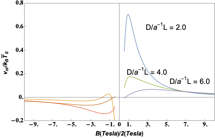
Figure 5: Normalized $[e\times$ non local voltage] vs $b=B/(2\>Tesla)$, at various distances from the origin: $D/a^{-1}L=2.,4.,6.,8$.

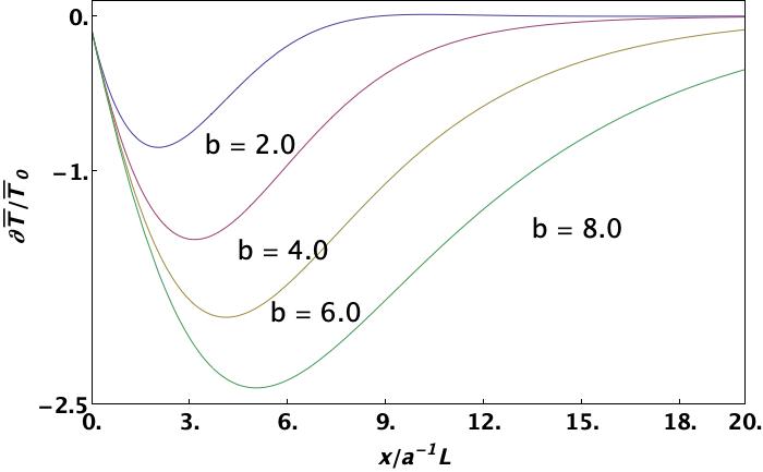
Figure 6: Normalized space derivative of the temperature vs distance $D/a^{-1}L$ from the origin, at different magnetic fields ($b=B/(2\>Tesla)=2.,4.,6.,8.$).

Figure 7: Normalized imbalance chemical potential $\delta\mu_{I}$ vs distance $D/a^{-1}L$ from the origin, at different magnetic fields ( $b=B/(2\>Tesla)=2.,4.,6.,8.$)

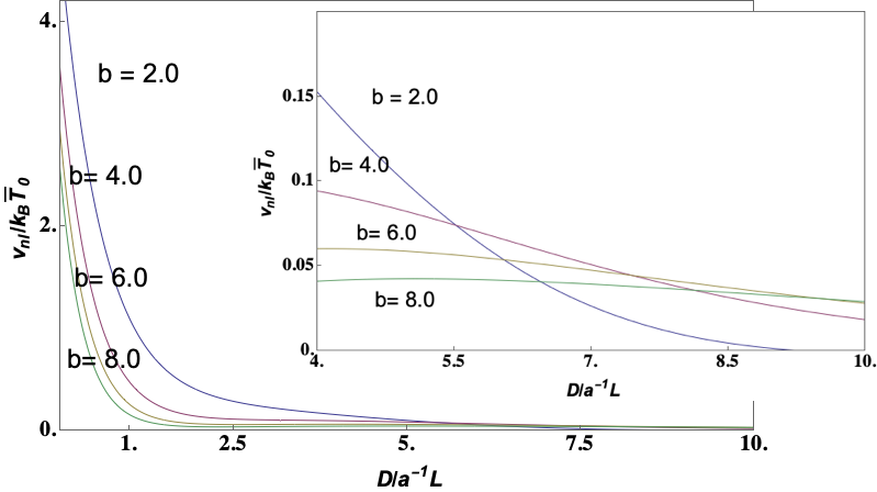
Figure 8: Normalized [$e\times$ non local voltage] vs distance from the origin $D/a^{-1}L$ at different magnetic fields ($b=B/(2\>Tesla)=2.,4.,6.,8.$). Inset: zooming of $[e\times$ non local voltage] at larger distances from the origin, at different magnetic fields ($b=B/(2\>Tesla)=2.,4.,6.,8.$)

Figure 9: Normalized imbalance chemical potential $\delta\mu_{I}$ vs distance $D/a^{-1}L$ from the origin, at different magnetic fields ($b=B/(2\>Tesla)=-2.,-4.,-6.,-8.$)

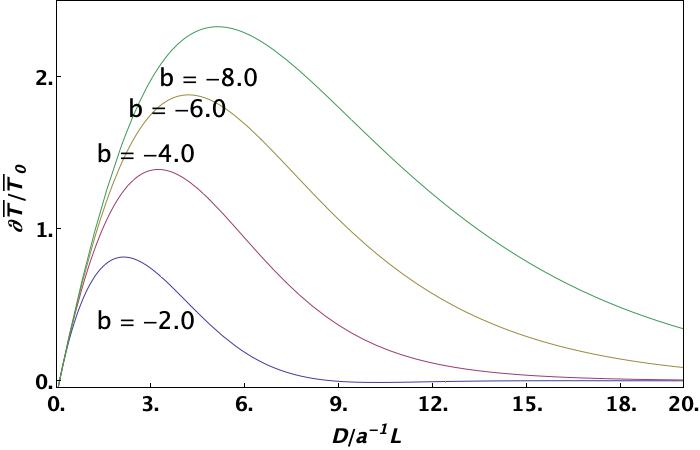
Figure 10: Normalized space derivative of the temperature vs distance $D/a^{-1}L$ from the origin, at different magnetic fields ($b=B/(2\>Tesla)=-2.,-4.,-6.,-8.$).

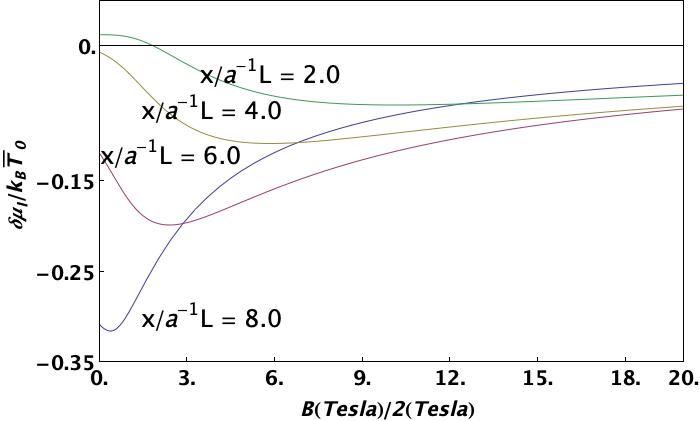
Figure 11: Normalized imbalance chemical potential $\delta\mu_{I}$ vs $b=B/(2\>Tesla)$ at various distances $D/a^{-1}L=2.,4.,6.,8.$ from the origin

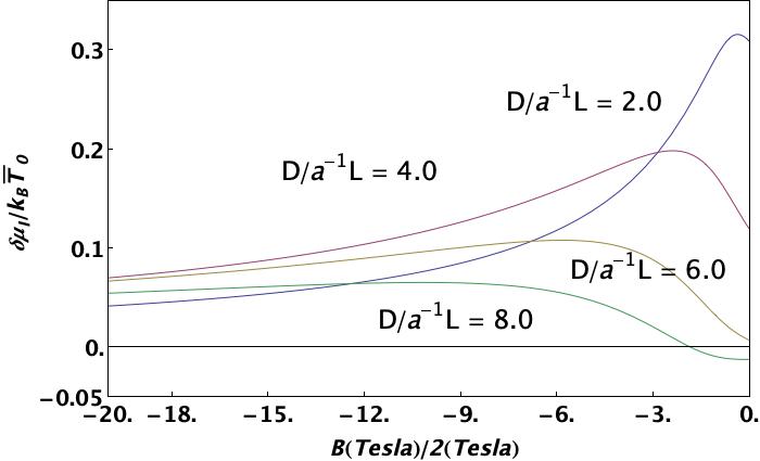
Figure 12: Normalized imbalance chemical potential $\delta\mu_{I}$ vs $b=B/(2\>Tesla)$ at various distances $D/a^{-1}L=2.,4.,6.,8.$ from the origin

The differential system is fully homogeneous. Unknown functions depend on an overall scale normalization. Close to the origin, the magnitude of $\partial_{x}\tau$ is determined by ${\cal{E}}$, field according to the Nernst boundary condition of Eq.(IV.12). This is the reason why we could extract the Ettingshausen parameter in the near zone. To extract the magnitude of the NLV away from the origin, the differential equation system should have been solved allowing for a selfconsistent ${\cal{E}}$ field at any distance ($\theta\to\theta(x)$) . This has not been done. Therefore, in the far zone the magnitude of the NLV is strictly speaking undetermined. We could try to use our estimate of the Ettingshausen parameter of Eq.(V.16) to determine the normalization, by using $nAmp$ as a probe current and $1\>Tesla$ as the reference magnetic field, and extracting a temperature derivative $\partial T/\partial(a^{-1}L)\approx 10^{-2}\>{}^{o}\!K/(a^{-1}L)$. However, when we plug this in Eq.(VI.3) and we evaluate the NLR by means of the same current, we find that our estimate is two-three orders of magnitude larger than the measured one, amounting to $k\Omega$s.

VII Summary and Final Remarks

Near the Dirac point, graphene Hall bars in an applied orthogonal magnetic field of the order of a few Tesla, exhibit large nonlocal resistances which cannot be fully explained within the framework of the “ideal” Quantum Hall Effect (QHE) in graphene. Here, we discuss nonlocal resistances in a Hall bar configuration corresponding to an open circuit in the longitudinal direction, parallel to the length of the Hall bar. In these conditions, one would expect zero voltage between contacts in the transverse direction, and that a transverse current injected at one boundary of the Hall bar, driven by an external electric field ${\cal{E}}$ gives rise to a local resistance that exponentially vanishes far from that boundary. Instead, the decay is power-law and there is a marked asymmetry between positive and negative values of the $B$ field, which is reduced at increasing distance from the injection point. Weak spin orbit coupling in graphene excludes that the NLR is due to Spin Hall Effect Bercioux and Lucignano (2015); Lucignano et al. (2008); Abanin et al. (2011b). The model of McEuen et al. McEuen et al. (1990) has been used by one of us and collaborators to describe qualitatively and semi-quantitatively the experimental resultsNachawaty et al. (2018). The model rests on the assumption that a non insulating bulk plays a role in transport close to the CNP. This is actually consistent with the model by Abanin et al.Abanin et al. (2011b), which we review in Section III and accounts for some dissipative effects measured in graphene at the CNP by assuming leakage of edge carriers into the bulk. The $\nu=0$ Landau level would be splitted by Zeeman interaction and a sort of plateaux in the $xy$-conductance would survive at the CNP accompanied by a sizeable longitudinal bulk resistance. Indeed, graphene on SiC, in which QHE was measured with a metrological precision, is relatively disordered, with strong intervalley scattering. However, these models are unable to catch the asymmetry under a change in sign of the applied the magnetic field.

In this work we have reconsidered the possibility that dissipation in the bulk can be accompanied by local charge imbalance and thermal gradients diffusing across the Hall bar, thus being responsible for the NLR. We can expect that even in the presence of relatively strong magnetic field, close to the CNP, in the high-mobility bulk graphene, the Fermi surface vanishes, leading to ineffective screening and linear energy dispersion, which implies the formation of a strongly-interacting quasi-relativistic electron- hole Dirac fluid Sheehy and Schmalian (2007).

In the relativistic approach, which is reviewed in Section II, particle current with energy transfer can be a neutral excitation mode independent of the charge transfer. The linear energy dispersion is also responsible for long recombination relaxation times of the quasiparticles, so that local charge imbalance can persist during the diffusion. We propose that the McEuen model accounts for the large part of the NLR, but long lived thermal effects occurring at low temperature in the bulk of the Hall bar may add a relevant contribution which, in particular, could be the source of the asymmetry when flipping $B$. In fact the McEuen model requires bulk conductivities $\sigma_{1},\sigma_{2}$ for particles and holes respectively, which are not the same.

On these side effects we focus on. At low temperature ($T\sim 1\>^{o}K$), with local non equilibrium induced by a locally applied transverse electric field, a few-Tesla $B$ induces space separation of oppositely charged carriers leaking from opposite edges, with little recombination relaxation rate. The charge imbalance generated in the bulk of the Hall bar by Joule heating close to the source is drifted far from the injection point by a Nernst thermal gradient at open circuit. In our framework, this is monitored by the space dependence of the imbalance chemical potential which does not decay exponentially along the Hall bar over distances comparable with the sample length. The bulk charge imbalance accumulated at opposite edges turns into a non local voltage that can be probed by an external transverse current which produces the NLR. The contribution discussed here appears in Fig.(5) and is strongly asymmetric under changing the sign of $B$.

Various remarks are in order.

As mentioned at the end of Section VI, we assume that the applied perturbation is localized close to the origin and only the drift of charges induced by the thermal gradient is accounted for in solving the diffusion equations derived in the hydrodynamical limit, far away from the injection point. Self-consistency is invoked to fix the non local voltage in the absence of sources. This implies that, far from the source, the set of differential equations is homogeneous and the solution is up to an unknown constant energy scale $k_{B}\overline{T}_{0}$. We have tried to estimate this constant in conjunction with the Ettingshausen parameter, but it can be of course fitted from experiment. Once the polarization of the electric field ${\cal{E}}$ is fixed, the response of the system to opposite directions of the applied $B$ field is certainly asymmetric, as particles are exchanged with holes when flipping the orientation of the magnetic field. The asymmetry is stronger close to the injection point. The asymmetry with $B$ found experimentally can help in fixing the ratio between the contribution coming from Eq.(VI.3) and the one coming from the McEuen model.

The charge imbalance arises from the spatial separation of charges, as it can be seen from the sketch of Fig.(2). In fact, the magnetic field tends to keep carriers of opposite sign far away from one another. This reduces the chances of recombination. However some charge imbalance also originates from the difference between the bulk conductivities $\sigma_{1},\sigma_{2}$ of the opposite charge carriers, which could be the source of a reduction of the Coulomb interaction between charges. This difference parametrized by the variable $q$ of Eq.(IV.15) increases the asymmetry with the magnetic field orientation as $q$ is odd with $B$ and appears explicitely on the r.h.s. of Eq.(VI.3). It is remarkable that, according to our model, the closer the bulk conductivities are, the longer is the decay length $\lambda$ of the NLV, as can be seen from Eq.(VI.4).

We assume that the Dirac model, in presence of two carriers of opposite charge (at the CNP), is the appropriate low energy framework to discuss the thermal, as well as the charge transport. Hence we only consider the lowest bath temperatures attained in the experiment which are $T\sim 1\div 1.7\>^{o}\!K$. In Eq.(V.7) an estimate is given of the charge imbalance chemical potential $\delta\mu_{I}$ in units $k_{B}\>^{o}\!K$ and is comparable with the bath temperature. Being estimated close to the origin, where the perturbation acts, $\delta\mu_{I}\sim 2$ appears as the maximum attainable value. Hence we are at the limit of validity for our approach, because, in this range of values, the Dirac model gives up by turning into the more appropriate Fermi Liquid model. In passing, we note that, at these temperatures, similar, but $p$ doped, graphene/SiC samples have been used as barrier for Al/graphene/Al superconducting Josephson junctions, showing a remarkable hysteretic loop of the critical current when the magnetic field is cycled and an Aslamazov-Larkin (AL) paraconductivity temperature dependence consistent with a Fermi Liquid pictureMassarotti et al. (2016, 2017).

In the Dirac model the relativistic stress energy tensor provides the energy flux $T^{0}_{\alpha}$ from the four-momentum conservation. The full approach does not contain more general dissipative terms except in Eq.(VI.3) for $v_{y}$, in which a phenomenological dissipative term has been added. The recombination time $\tau_{Q}\sim 1/\sqrt{B}$ has been measured and found rather longRana (2007); Winnerl et al. (2011). This extra term has been added to account for the relatively fast decay of $v_{y}$ with increasing $B$. If we neglect this term, the decay is determined by $\lambda$ given by Eq.(VI.4) which gives a weaker dependence on $B$.

The numerical values for the electrical bulk conductivities are derived from Ref.[Nachawaty et al., 2018], while the numerical values chosen for the thermal transport 3-d parameters (Nernst and Peltier parameters, thermal conductivity) have been found in the literature. In various occasions we have compared those values with the ones derived from 3-d hydrodynamics of a Fermi LiquidMüller et al. (2008); Müller and Sachdev (2008). This has given us the chance of fixing the order of magnitude of two quantities that are relevant in thermal transport, but are difficult to extract from experiment: the enthalpy per particle $eQ$ and the particle density in the effective 3-d system $n_{3d}$. Thermal transport is an essentially 3-d phenomenon and the knowledge of the sheet carrier density of graphene $n_{\square}$, as determined by the QHE, is not enough. The value we have chosen for $eQ$ is not far from $k_{B}T$ plus the magnetization work $-M\>B$ which freezes the kinetic energy term. This reduces $\lambda$ with increasing $B$.

Our results cannot be valid in the limit of small magnetic field ($B\lessapprox 1\>Tesla$). Outside of the QHE regime the model, in the absence of edge modes, is invalid from the outset. However the trend when the magnetic field is reduced is qualitatively well represented by our results of Fig.(5). Of course the transport parameters should be recalculated in a Dirac frame and in presence of QHE quantization of the conductivity. Nevertheless, hydrodynamics is still valid at very low energy (very low temperatures), lower that the Zeeman splitting at $\nu=0$. The starting guess is that the bulk of the Hall bar is not totally insulating even at such a small working temperature.

We conclude by noting that further studies of the thermal transport in chemical vapour deposited graphene can help by making the fractional quantum Hall effect an efficient and controlled playground for applications in alternative quantum information processors.

Appendix A Diffusion equation for the average temperature $\overline{T}$

Here we derive the diffusion equation for the temperature $\overline{T}(x)$, induced by the imbalance charge $\rho_{I}(x)$ defined in Eq.(IV.6), $\rho_{I}=n_{\square}\left(c_{+,A}-c_{+,B}-2\>s_{+}\right)$.

Using the notation introduced in Section III, We assume the mirror symmetry between the side $A$ and $B$ of the bar, so that $s_{+}=s_{+,A}=-s_{+,B}$ in the following.

Solving Eq.s(IV.5) with respect to the potentials $"s"$, we get ($Q\equiv\left(\frac{\epsilon+{\cal{P}}}{n\>e}\right)_{3d}$)

$$s_{-,A}-s_{-,B}=-K_{-}\>\left(-\partial_{x}\Delta T\right)-\frac{w}{4}\left(\frac{1}{\sigma_{1}}-\frac{1}{\sigma_{2}}\right)\alpha_{xy}\Delta T\>\frac{{\cal{E}}\>}{Q}-\frac{w}{4}\left(\frac{1}{\sigma_{1}}+\frac{1}{\sigma_{2}}\right)g\>\frac{2\gamma}{2\gamma+g}\>(s_{-,A}+s_{-,B})$$ (A.1)

$$s_{-,A}+s_{-,B}=-K_{-}(-\nabla_{x}\overline{T})-\frac{w}{4}\>\left(\frac{1}{\sigma_{1}}-\frac{1}{\sigma_{2}}\right)\>\alpha_{xy}\overline{T}\>\frac{{\cal{E}}\>}{Q}-g\>\frac{2\gamma}{2\gamma+g}\>\frac{w}{4}\>\left(\frac{1}{\sigma_{1}}+\frac{1}{\sigma_{2}}\right)\>\left(s_{-,A}-s_{-,B}\right)$$ (A.2)

$$2s_{+}=-K_{+}(-\nabla_{x}\overline{T})-\frac{w}{4}\left(\frac{1}{\sigma_{1}}+\frac{1}{\sigma_{2}}\right)\>\alpha_{xy}\overline{T}\>\frac{{\cal{E}}\>}{Q}-\frac{w}{4}\left(\frac{1}{\sigma_{1}}-\frac{1}{\sigma_{2}}\right)g\>\frac{2\gamma}{2\gamma+g}\>\left(s_{-,A}-s_{-,B}\right)\;,$$ (A.3)

where

$$K_{\pm}=\frac{w}{4}\left[\left(\frac{1}{\sigma_{1}}\pm\frac{1}{\sigma_{2}}\right)\frac{\kappa_{xx}}{Q}+\left(\frac{1}{\sigma_{1}}\mp\frac{1}{\sigma_{2}}\right)\>\alpha_{yx}\right].$$ (A.4)

Singling out the $-2\partial_{x}s_{+}$ term from Eq.(IV.7) and substituting it into the derivative of Eq.(A.3), one gets:

$$K_{+}(-\nabla^{2}_{x}\overline{T})+\frac{w}{4}\left(\frac{1}{\sigma_{1}}+\frac{1}{\sigma_{2}}\right)\alpha_{xy}\nabla_{x}\left(\overline{T}\>\frac{{\cal{E}}\>}{Q}\right)+\frac{w}{4}\left(\frac{1}{\sigma_{1}}-\frac{1}{\sigma_{2}}\right)g\>\frac{2\gamma}{2\gamma+g}\>\partial_{x}\left(s_{-,A}-s_{-,B}\right)$$

$$=\frac{\sigma_{1}-\sigma_{2}}{\sigma_{1}+\sigma_{2}}\>\partial_{x}\left(s_{-,A}+s_{-,B}\right)-\frac{2\>v_{F}\>w}{(\sigma_{1}+\sigma_{2})}\>\frac{1}{n_{\square}{\cal{V}}}\rho_{I}.$$

In the comparison with the derivative of Eq.(A.2):

$$\partial_{x}\left(s_{-,A}+s_{-,B}\right)=-K_{-}(-\nabla^{2}_{x}\overline{T})-\frac{w}{4}\left(\frac{1}{\sigma_{1}}-\frac{1}{\sigma_{2}}\right)\alpha_{xy}\nabla_{x}\left(\overline{T}\frac{{\cal{E}}}{Q}\right)-g\>\frac{2\gamma}{2\gamma+g}\frac{w}{4}\>\left(\frac{1}{\sigma_{1}}+\frac{1}{\sigma_{2}}\right)\partial_{x}\left(s_{-,A}-s_{-,B}\right),$$ (A.5)

the contribution from $\partial_{x}(s_{-,A}-s_{-,B})$ cancels out, giving eventually the final form of the equation we are looking after:

$$\kappa_{xx}\>(-\nabla^{2}_{x}\overline{T})+\alpha_{xy}\nabla_{x}\left(\overline{T}\>{\cal{E}}\right)=-4\>\left(\frac{\epsilon+{\cal{P}}}{n\>e^{2}}\right)_{3d}\>\frac{1}{n_{\square}{\cal{V}}}\>v_{F}\>\frac{\sigma_{1}\sigma_{2}}{(\sigma_{1}^{2}+\sigma_{2}^{2})}\>\rho_{I},$$ (A.6)

which can be cast in the form ($\theta\equiv{\alpha_{xy}\>{\cal{E}}\>L}/{\kappa_{xx}}$):

$$\partial^{2}_{\tilde{x}}\tau-\theta\>\partial_{\tilde{x}}\tau=\tilde{\beta}\delta\mu_{I},$$ (A.7)

$$\tilde{\beta}=\left(\frac{\epsilon+{\cal{P}}}{n\>e^{2}}\right)_{3d}\>\frac{v_{F}}{n_{\square}{\cal{V}}}\>\frac{k_{B}}{\kappa_{xx}}\>\frac{4\>\sigma_{1}\sigma_{2}}{(\sigma_{1}^{2}+\sigma_{2}^{2})}\times\left[1-\left(\frac{\sigma_{B}}{\sigma_{3d}}\right)^{2}\right]^{-1}\>,$$

(A.8)

where $\delta\mu_{I}=\frac{e\rho_{I}L^{2}}{k_{B}\>^{o}K}$ and $\tau=\overline{T}/\>^{o}K$.

Appendix B Equation for the imbalance energy $\delta\mu_{I}$

We now derive the equation that relates the imbalance energy $\delta\mu_{I}$ to the average temperature $\overline{T}$. From Eq.s(IV.1), we get:

$$\partial_{x}(c_{+,A}-c_{+,B}) =-(2\>\gamma^{\prime}+g^{\prime})(c_{-,A}+c_{-,B})+g^{\prime}(s_{-,A}-s_{-,B})$$ (B.9)

$$\partial_{x}(c_{-,A}-c_{-,B}) =-g^{\prime}\>(c_{+,A}+c_{+,B})$$ (B.10)

$$\partial_{x}(c_{+,A}+c_{+,B}) =-(2\>\gamma^{\prime}+g^{\prime})(c_{-,A}-c_{-,B})+g^{\prime}(s_{-,A}+s_{-,B})$$ (B.11)

$$\partial_{x}\left(c_{-,A}+c_{-,B}\right) =-g^{\prime}\>\left[c_{+,A}-c_{+,B}-2\>s_{+}\right]$$ (B.12)

$$\partial^{2}_{x}(c_{-,A}-c_{-,B}) =g^{\prime}\>(2\gamma^{\prime}+g^{\prime})(c_{-,A}-c_{-,B})-{g^{\prime}}^{2}\>(s_{-,A}+s_{-,B})$$

$$\partial^{2}_{x}(c_{+,A}-c_{+,B}) =g^{\prime}\>(2\gamma^{\prime}+g^{\prime})\left[c_{+,A}-c_{+,B}-2s_{+}\right]+g^{\prime}\>\partial_{x}(s_{-,A}-s_{-,B})$$ (B.13)

Using Eq.(B.13) and Eq.(IV.7), we also obtain:

$$\partial_{x}\left(c_{+,A}-c_{+,B}-2\>s_{+}\right)=-(2\gamma+g)\>t_{0}\>(c_{-,A}+c_{-,B})+g\>t_{0}\>\left(s_{-,A}-s_{-,B}\right)$$

$$-\frac{2\>w\>v_{F}}{(\sigma_{1}+\sigma_{2}){\cal{V}}}\>\left(c_{+,A}-c_{+,B}-2\>s_{+}\right)+\frac{\sigma_{1}-\sigma_{2}}{\sigma_{1}+\sigma_{2}}\>\partial_{x}\left(s_{-,A}+s_{-,B}\right)$$ (B.14)

The parameters $g$ and $\gamma$ have dimensions $[1/(Lt_{0})]$ where $t_{0}$ is the relaxation time scale that we have introduced in the definition of the dimensionless leakage parameter from the edge states to the bulk, $\tilde{g}=g(2\>\gamma+g)L^{2}t_{0}^{2}$ to properly match the dimensions ( see below for details). By differentiating Eq.(B.14) and by plugging into it Eq.s(A.1), keeping terms up to ${\cal{O}}(g^{2})$, one recovers the desired equation, connecting the imbalance potential with the thermal excess temperatures, given by:

$$\partial^{2}_{x}\left(c_{+,A}-c_{+,B}-2\>s_{+}\right)+\frac{2\>w\>\>v_{F}}{(\sigma_{1}+\sigma_{2}){\cal{V}}}\>\partial_{x}\left(c_{+,A}-c_{+,B}-2\>s_{+}\right)-g\>(2\gamma+g)\>\tau_{Q}^{2}\left(c_{+,A}-c_{+,B}-2\>s_{+}\right)$$

$$+\frac{\sigma_{1}-\sigma_{2}}{\sigma_{1}+\sigma_{2}}\>\partial_{x}^{2}\left\{K_{-}(-\partial_{x}\overline{T})+\frac{w}{4}\>\left(\frac{1}{\sigma_{1}}-\frac{1}{\sigma_{2}}\right)\>\frac{\alpha_{xy}\>{\cal{E}}}{Q}\>\overline{T}\right\}$$

$$=-g\>\tau_{Q}\left[1-\frac{2\gamma\>\tau_{Q}^{-1}}{2\gamma+g}\>\frac{w}{4}\>\left(\frac{1}{\sigma_{1}}+\frac{1}{\sigma_{2}}\right)\>\frac{\sigma_{1}-\sigma_{2}}{\sigma_{1}+\sigma_{2}}\right]\>\partial_{x}\left\{K_{-}\left(-\partial_{x}\Delta T\right)+\frac{w}{4}\left(\frac{1}{\sigma_{1}}-\frac{1}{\sigma_{2}}\right)\>\frac{\alpha_{xy}\>{\cal{E}}}{Q}\>\Delta T\right\},$$ (B.15)

Note that the expression in curly brackets is the same, both for $\overline{T}$ and for $\Delta T$. One can assume that one of the two is constant. We neglect any $\hat{y}-$dependence of $\rho_{I}$ except for the mirror symmetry, so to make it independent of $\Delta T=T_{A}-T_{B}$. Hence the right hand side is put equal to zero:

$$K_{-}\left(-\partial_{x}\Delta T\right)+\frac{w}{4}\left(\frac{1}{\sigma_{1}}-\frac{1}{\sigma_{2}}\right)\>\frac{\alpha_{xy}\>{\cal{E}}}{Q}\>\Delta T=cnst,$$ (B.16)

where the constant can be put to zero. Our choice is consistent with the initial choice $s_{+,A}=-s_{+,B}=s_{+}$. Finally, multiplying both sides by $e\>n_{\square}L^{2}/k_{B}\>^{o}K$ and resorting to the dimensionless space coordinate ${\tilde{x}}=x/L$, we get:

$$\partial^{2}_{\tilde{x}}\delta\mu_{I}+\frac{2\>w\>L\>v_{F}}{(\sigma_{1}+\sigma_{2}){\cal{V}}}\>\partial_{\tilde{x}}\delta\mu_{I}-\tilde{g}\>\delta\mu_{I}=-\frac{e}{k_{B}}\frac{n_{\square}L^{2}}{Q}\>\frac{\sigma_{1}-\sigma_{2}}{\sigma_{1}+\sigma_{2}}\>\frac{w}{4\>L}\>\partial^{2}_{\tilde{x}}\left[\left\{\left(\frac{1}{\sigma_{1}}-\frac{1}{\sigma_{2}}\right)\>\kappa_{xx}\right.\right.$$

$$\left.\left.+\left(\frac{1}{\sigma_{1}}+\frac{1}{\sigma_{2}}\right)\>\alpha_{yx}\>Q\right\}(-\partial_{\tilde{x}}\tau)+\left(\frac{1}{\sigma_{1}}-\frac{1}{\sigma_{2}}\right)\>\kappa_{xx}\>\left(\frac{\alpha_{xy}}{\kappa_{xx}}\>{\cal{E}}\>L\right)\>\tau\right].$$ (B.17)

Appendix C Fermi liquid transport parameters

The scattering time is the $e-e$ inelastic one, because this is the time scale which qualifies the imbalance relaxation rate: $\tau_{ee}^{-1}=\alpha_{f}^{2}\>k_{B}T/\hbar$. The elastic scattering is unable to relax the charge imbalance. At $B=2\>Tesla$, one gets:

$$\omega_{c}\tau=\frac{eB}{c}\frac{v_{F}}{\hbar k_{F}}\tau_{ee}=0.4626\times 10^{6}\>,$$

with $k_{F}=(\pi\>n_{\square})^{1/2}$ and $n_{\square}=10^{10}/cm^{2}$, $v_{F}=c/300$, $B=2\>Tesla$.

In terms of the enthalpy, the thermal response functions in the limit $\omega_{c}\tau>>1$ are given by Eq.s(II.18,II.20). In the Fermi liquid regime, in which the thermal energy is lower than the chemical potential, the expressions for the transport coefficients $\alpha_{xy}^{FL}$ and $\kappa_{xx}^{FL}$ are:

$$\alpha_{xy}^{FL}=\left(\frac{\epsilon+{\cal{P}}}{n\>e}\right)_{3d}\>\frac{\sigma_{B}}{T}.$$

$$\kappa_{xx}^{FL}\approx\left(\frac{\epsilon+{\cal{P}}}{n\>e}\right)_{3d}^{2}\frac{\sigma_{3d}}{T}\left[1-\left(\frac{\sigma_{B}}{\sigma_{3d}}\right)^{2}\right].$$ (C.18)

These are quantities defined in 3-d, where their 3 dimensions are respectively given by $[\alpha]\sim e/(Lt\>T)$ and by $[\kappa]\sim e^{2}/(L^{2}\>t\>T)$. On the other hand, in the range $T=1\div 10\>^{o}\!K$ the value reported for graphene is Checkelsky and Ong (2009) $\alpha_{xy}\approx 75\>nAmp/^{o}K$, which is a 2-d quantity. As we consider thermal effects in the graphene grown onto SiC as a ”bulk ” phenomenon, we extend the definition of $\alpha_{xy}$ to $3d$ by dividing it by $\sim 0.3\>nm$, so that we eventually obtain:

$$\alpha_{xy}\approx 2.24\times 10^{11}V/(^{o}K\>sec).$$ (C.19)

Ref.[Müller and Sachdev, 2008] provides a numerical estimate $\left(\epsilon+{\cal{P}}\right)_{\square}\sim 0.12\times 10^{3}\>(T/\>^{o}K)^{3}\>eV/cm^{2}$, also given in Ref.[Crossno et al., 2016], when the chemical potential exceeds thermal energy, even at temperature $40\>^{o}K$. The question is how to relate this quantity to the corresponding 3-d quantity$\left(\epsilon+{\cal{P}}\right)_{3d}$, that is required for the enthalpy per unit (3-d) volume.

We make the following choice. We define a total energy per particle by multiplying $\left(\epsilon+{\mathcal{P}}\right)_{3d}$ by the volume ${\mathcal{V}}=\ell w\times 1\AA\approx 10^{-11}cm^{3}$ and dividing it by the effective number of 3-d carriers ${\cal{N}}_{3d}\sim 10^{3}$ and we pose:

$$Q=\frac{\left(\epsilon+{\cal{P}}\right)_{3d}{\cal{V}}}{{\cal{N}}_{3d}\>e}\approx 0.12\times 10^{-3}\>V$$ (C.20)

(here and in the following $V\equiv Volt$). We will show that this value for ${\cal{N}}_{3d}$ is also suggested by our self consistent procedure. ${\cal{N}}_{3d}$ can be interpreted as the effective number for carriers contributing to the thermal processes in the 3-d strip. This value for ${\cal{N}}_{3d}$ allows us to match reasonably well the values from a Fermi Liquid approach of Eq.(C.18) and those experimentally found for $\alpha_{xy}$, $\kappa_{xx}$ and $e_{N}$. The value reported by experimentalists for $\kappa_{xx}$,adopted by us, is $\kappa_{xx}\approx 1\div 10\>Watt/(^{o}K\times meter)$ .

The ratio $\kappa_{xx}^{FL}/\alpha_{xy}^{FL}$ is given by:

$$\frac{\kappa_{xx}^{FL}}{\alpha_{xy}^{FL}}=\left(\frac{\epsilon+{\cal{P}}}{n\>e}\right)_{3d}\frac{\sigma_{3d}}{\sigma_{B}}\left[1-\left(\frac{\sigma_{B}}{\sigma_{3d}}\right)^{2}\right],$$ (C.21)

As $\sigma_{3d}L^{d-2}=R^{-1}$, an aspect ratio is required, so that $\sigma_{3d}^{-1}=R\ell d/w\approx 0.5\times 10^{-15}\>sec$, with $d=1\AA$ and $R=10\>k\Omega$. Here $R$ is the longitudinal resistance and $\ell w$ the area.

Here $\sigma_{B}/\sigma_{3d}=e^{2}R/h\cdot[hc/(eB\ell w)]\cdot\ell/w$(note that, as it happens in the hydrodynamic approach, the limits $B\to 0$ and $\omega\to 0$ do not commute). We find

$$\sigma_{B}=\frac{{\cal{N}}_{3d}}{{\cal{V}}}\frac{e\>c}{B}\approx 2.4\times\frac{10^{15}}{cm^{3}}.\frac{ec}{B}.$$

$$=0.84\times 10^{12}sec^{-1}$$ (C.22)

With these conductances, the ratio of Eq.(C.21) is estimated as:

$$\frac{\kappa_{xx}^{FL}}{\alpha_{xy}^{FL}}\approx 4.\times 10^{-2}\>V$$ (C.23)

The Nernst coefficient in the limit of large fields and relatively clean samplesCheckelsky and Ong (2009) is $e_{N}^{3d}=(\sigma^{-1}\alpha)_{xy}\approx 1\>mV/^{o}K$.

Appendix D Coupled differential equation and relaxational scales

Let us rearrange the system of differential equations involving $\bar{T}$ and $\delta\mu_{I}$, Eq.(A.7) and Eq.(B.17), in a more practical form so to be able to discuss the relaxation length scale of the two unknown functions in the $\hat{x}-$direction.

We write the prefactor of $(-\partial_{\tilde{x}}\tau)$ as $k\equiv u\>k_{u}$ where $k_{u}$ is given by:

$$k_{u}=1+\left(\frac{\sigma_{1}+\sigma_{2}}{\sigma_{2}-\sigma_{1}}\right)\>\frac{\alpha_{yx}}{\kappa_{xx}}\>Q,$$ (D.24)

and $u$ is given by:

$$u=\frac{e}{k_{B}}\frac{n_{\square}L^{2}}{Q}\frac{\sigma_{1}-\sigma_{2}}{\sigma_{1}+\sigma_{2}}\>\frac{w}{4\>L}\>\left(\frac{1}{\sigma_{1}}-\frac{1}{\sigma_{2}}\right)\>\kappa_{xx}$$ (D.25)

Eq.s(IV.13) follow:

$$\partial^{2}_{\tilde{x}}\>\tau-\partial_{\tilde{x}}\>\left(\theta\>\tau\right)=\tilde{\beta}\>\delta\mu_{I},\>\>\>(a)\>\>\>\>$$

$$\partial^{2}_{\tilde{x}}\>\delta\mu_{I}+a\>\partial_{\tilde{x}}\>\delta\mu_{I}-\tilde{g}\>\>\delta\mu_{I}=\partial^{2}_{\tilde{x}}\>\left\{k\>\partial_{\tilde{x}}\>\tau-\theta\>u\>\tau\right\}.\>\>\>(b)$$

(D.26)

A numerical solution is obtained by deriving an equation for $\delta\mu_{I}$ only and by inserting the solution into Eq(D.26,(a)). Multiplying Eq.(D.26,(a)) by $k$ and substituting it in Eq.(D.26,(b)) , we get:

$$(k-u)\>\partial^{2}_{\tilde{x}}\left(\theta\>\tau\right)=\partial^{2}_{\tilde{x}}\>\delta\mu_{I}+(a-k\tilde{\beta})\>\partial_{\tilde{x}}\>\delta\mu_{I}-\tilde{g}\>\delta\mu_{I}$$

(D.27)

From now on we shift $a\to a-u\tilde{\beta}$ by summing and subtracting $u\tilde{\beta}$ to $a$, and ridefine it as $a$ thus obtaining:

$$(k-u)\>\partial^{2}_{\tilde{x}}\left(\theta\>\tau\right)=\partial^{2}_{\tilde{x}}\>\delta\mu_{I}+[a-(k-u)\tilde{\beta}]\>\partial_{\tilde{x}}\>\delta\mu_{I}-\tilde{g}\>\delta\mu_{I}.$$

(D.28)

We cast the system in length units $a^{-1}L$: ($\tilde{{\tilde{x}}}=x/(a^{-1}L)$ and introduce the new variables $\mu^{\prime}\equiv\tilde{\beta}a^{-1}\delta\mu_{I}$, $\tau^{\prime}\equiv a\>\tau$ to get:

$$\partial^{2}_{\tilde{{\tilde{x}}}}\>\tau^{\prime}-\partial_{\tilde{{\tilde{x}}}}\>\left(\theta a^{-1}\>\tau^{\prime}\right)=\mu^{\prime},\>\>\>\>\>(a)$$

$$\partial^{2}_{\tilde{{\tilde{x}}}}\>\mu^{\prime}+\partial_{\tilde{{\tilde{x}}}}\>\mu^{\prime}-\tilde{g}a^{-2}\>\>\mu^{\prime}\>\>\>\>\>\>\hskip 113.81102pt$$ (D.29)

$$=\partial^{2}_{\tilde{{\tilde{x}}}}\>\left\{(\tilde{\beta}ka^{-1})\>\partial_{\tilde{{\tilde{x}}}}\>\tau^{\prime}-\theta a^{-1}\>(\tilde{\beta}ua^{-1})\>\tau^{\prime}\right\}.\>(b)$$

where

$$a\equiv 2\>\frac{w}{(\sigma_{1}+\sigma_{2}){\cal{V}}}\>v_{F},\>\>\>\>\tilde{g}\equiv g(2{\gamma}+g)\>L^{2}t_{0}^{2}.$$ (D.30)

The Fermi velocity $v_{F}=c/300=10^{8}\>cm/sec$. We take the parameter that describes the leakage from edge to bulk $\tilde{g}\sim 10^{-6}$, so that $\tilde{g}a^{-2}\sim 10^{0}$ .

For $\tilde{\beta}\sim 10^{-9}$ and $a\sim 10^{-3}$ Eq.(D.24) and Eq.(D.25) give ( see in the next, Subsection D)

$$k^{\prime}\equiv\tilde{\beta}k\>a^{-1}=q^{2}+3\times 10^{-3}\>q$$

$$u^{\prime}\equiv\tilde{\beta}u\>a^{-1}=q^{2},\>\>\>\>\>q=\frac{\sigma_{1}-\sigma_{2}}{[\sigma_{1}^{2}+\sigma_{2}^{2}]^{1/2}}.$$

(D.31)

The order of magnitude of $\theta$ is fixed by the applied voltage (expressed in $Volts\>\equiv V$), as derived from the experiment:

$${\cal{E}}w\>\sim 10^{-4}V\to R\sim\frac{10^{-4}V}{10\>n\>Amp}\sim 10\>k\Omega$$

$$\to\theta^{\prime}\equiv\theta\>a^{-1}=\frac{\alpha_{xy}}{\kappa_{xx}}\>{\cal{E}}w\>\frac{a^{-1}L}{w}\approx 3\times 10^{-2}.$$ (D.32)

The final equation is:

$$\partial^{2}_{\tilde{\tilde{x}}}\mu^{\prime}+\left[1-(k^{\prime}-u^{\prime})-\theta^{\prime}\right]\partial_{\tilde{\tilde{x}}}\mu^{\prime}$$

$$+\left(g^{\prime}+\theta^{\prime}\right)\mu^{\prime}-g^{\prime}\theta^{\prime}\int\mu^{\prime}d{\tilde{\tilde{x}}}=0$$ (D.33)

Appendix E Properties of the imbalance charge energy solution

Having discussed the order of magnitudes and the general features of the solutions of the system Eq.(D.26), we now turn to a numerical solution to highlight the dependence of $\delta\mu_{I}(x)$ and $\tau(x)$ on the magnetic field $B$, both far from $x=0$ and close to the origin.

We have shown in Appendix D that the system of Eq.(D.26) allows for a rewriting with parameters and unknown functions of ${\cal{O}}(1)$. The system of Eq.(D.29) has been used in the numerical results which are discussed in Section V of the text.

$$\partial^{2}_{\tilde{{\tilde{x}}}}\>\tau^{\prime}-\partial_{\tilde{{\tilde{x}}}}\>\left(\theta^{\prime}\>\tau^{\prime}\right)=\mu^{\prime},\>\>\>\>\>(a)$$

$$\partial^{2}_{\tilde{{\tilde{x}}}}\>\mu^{\prime}+\partial_{\tilde{{\tilde{x}}}}\>\mu^{\prime}-\tilde{g}^{\prime}\>\>\mu^{\prime}\>\>\>\>\>\>\hskip 113.81102pt$$ (E.34)

$$=\partial^{2}_{\tilde{{\tilde{x}}}}\>\left\{k^{\prime}\>\partial_{\tilde{{\tilde{x}}}}\>\tau^{\prime}-\theta^{\prime}u^{\prime}\>\tau^{\prime}\right\}.\>(b)$$

with $\tilde{g}^{\prime}=\tilde{g}a^{-2}$ and primed parameters given in Eq.(D.31, D.32). As discussed in the text, the solution of the homogeneous equation Eq.(E.34, (b)) has to be added to the solution of the system of coupled equations.

Here we keep the form of the system given in Eq.(E.34), but we drop all the primes for simplicity and we use $\partial$ instead of $\partial_{\tilde{{\tilde{x}}}}$.

For $g,\theta\neq 0$, a numerical solution is obtained by deriving an equation for $\mu$ only and, by inserting the solution into Eq(D.26,(a)). Multiplying Eq.(D.26,(a)) by $k$ and substituting it in Eq.(D.26,(b)) , we get:

$$(k-u)\>\partial^{2}\left(\theta\>\tau\right)=\partial^{2}\>\mu+[1-(k-u)]\>\partial\>\mu-g\>\mu$$

(E.35)

Let us consider $\partial\>\left(\theta\>\tau\right)=\theta\>\partial\>\tau+\tau\>\partial\>\theta$. The second term on the r.h.s. is reminiscent of $\partial_{\tilde{x}}\>{\cal{E}}_{y}-\partial_{\tilde{y}}\>{\cal{E}}_{x}$ where ${\cal{E}}_{x}=0$ because, in the bulk, the circuit is open ( no current along $x$ ) and assumed to be equipotential. This $z-$ component of $\vec{\nabla}\times\vec{{\cal{E}}}$ vanishes, because there is no current in the $z$ direction. We conclude that only the first term survives with a $\theta$ which is practically constant in $x$, in an interval of size $\theta^{-1}L$ close to the origin, or zero for any $x$ far from the origin. Following Eq.(E.34, E.35), we define

$$\>\>\>\>\>\>\>\>\>\>\>\>\nu(\tilde{x})=\nu_{0}+\int^{\tilde{x}}_{0}\!\!\!\mu(\tilde{x}^{\prime})\>d\tilde{x}^{\prime}$$ (E.36)

and we get:

$$\left\{\begin{array}[]{l}\partial^{2}\>\tau-\theta\>\partial\>\tau=\mu,\\ (k-u)\>\theta\>\partial\>\tau=\partial\>\mu+[1-(k-u)]\mu-g\>\nu\\ \partial\>\nu=\mu\end{array}\right.$$ (E.39)

or, substituting the second into the first:

$$\left\{\begin{array}[]{l}(k-u)\>\partial^{2}\>\tau=\partial\>\mu+\mu-g\>\nu,\\ (k-u)\>\theta\>\partial\>\tau=\partial\>\mu+[1-(k-u)]\>\mu-g\>\nu\\ \partial\>\nu=\mu\end{array}\right.$$ (E.41)

We now multiply the first equation by $\theta$ and differentiate the second one. Equating the two of them to each other, we obtain:

$$\partial^{2}_{\tilde{x}}\>\mu+(a-k\>\tilde{\beta})\>\partial_{\tilde{x}}\mu-\tilde{g}\>\mu=\theta\>\partial_{\tilde{x}}\>\mu+\theta\>\left(a-u\tilde{\beta}\right)\>\mu-\tilde{g}\>\theta\>\nu.$$

When $\mu$ has been found, one can plug it into the first one of Eq.s(E.39) to find $\partial_{\tilde{x}}\>\tau$. The equation can be written as a first order differential system:

$$\left\{\begin{array}[]{ll}\partial_{\tilde{x}}\>\mu&=\xi\\ \partial_{\tilde{x}}\>\nu&=\mu\\ \partial_{\tilde{x}}\>\xi&=-[1-(k-u)-\theta]\>\xi+[{g}+\theta]\>\mu-{g}\>\theta\>\nu,\end{array}\right.$$ (E.45)

or, in the matrix form,

$$\left(\begin{array}[]{c}\partial\>\mu\\ \partial\>\nu\\ \partial\>\xi\end{array}\right)=\left(\begin{array}[]{ccc}0&0&1\\ 1&0&0\\ G&-{g}\theta&-F\end{array}\right)\left(\begin{array}[]{c}\mu\\ \nu\\ \xi\end{array}\right)$$ (E.55)

with $F=1-(k-u)-\theta$ and $G={g}+\theta$. As discussed above, $a\to aa^{-1}\sim 1$, $k\tilde{\beta}\to k\tilde{\beta}a^{-2}$, $\tilde{g}\to\tilde{g}a^{-2}$, $u\tilde{\beta}\to u\tilde{\beta}a^{-2}$ and $\theta$ are all ${\cal{O}}(1)$. The characteristic equation giving the space dependence of the functions here $e^{\tilde{\lambda}\tilde{x}}$ is

$$\tilde{\lambda}^{3}+F\>\tilde{\lambda}^{2}-G\>\tilde{\lambda}+\tilde{g}\>\theta=0$$ (E.56)

For $\theta\neq 0$, solutions converging at infinity require $\tilde{g},\theta<0$.

The vanishing of the imbalance parameter $q$ implies the vanishing of $(k-u)$. Here we show that, for $\theta\neq 0$, the vanishing of $q$, provides two real or complex conjugate solutions for $\tilde{\lambda}$ which are independent of $\theta$ and a real solution $z_{3}=-\theta\>sign[\tilde{g}]$.

If $z_{1},z_{2},z_{3}$ are the roots of the cubic equation the following relations hold:

$$z_{1}z_{2}+z_{1}z_{3}+z_{2}z_{3}=-G,$$

$$z_{1}+z_{2}+z_{3}=-F,\>z_{1}z_{2}z_{3}=-\tilde{g}\theta.$$ (E.57)

Given $z_{1,2}=-a/2\pm\sqrt{(1-4|{g}|}/2$, it is easily found that $z_{3}=-\theta\>sign[{g}]$ satisfy Eq.s(E.57). When $q\neq 0$, one solution will be real and the other two will be complex or all of them will be real.

Appendix F The non local voltage

The equation for the non local voltage, in dimensionless units $v_{y}=e\>(c_{+,A}-c_{+,B})/(k_{B}\>^{o}K)$ is derived as follows.

We go back to Eq.(B.13):

$$\partial^{2}_{x}(c_{+,A}-c_{+,B}) =g^{\prime}\>(2\gamma^{\prime}+g^{\prime})\left[c_{+,A}-c_{+,B}-2s_{+}\right]+g^{\prime}\>\partial_{x}(s_{-,A}-s_{-,B}).$$

Inserting Eq.(A.1) and Eq.(A.3) in it, we get ( $T\approx 1\>^{o}\!K$):

$$\partial^{2}_{x}(c_{+,A}-c_{+,B})-g^{\prime}\>(2\gamma^{\prime}+g^{\prime})(c_{+,A}-c_{+,B})\hskip 227.62204pt$$

$$=g^{\prime}\left\{-K_{-}\>\left(-\partial_{x}^{2}\Delta T\right)-\frac{w}{4}\left(\frac{1}{\sigma_{1}}-\frac{1}{\sigma_{2}}\right)\alpha_{xy}\partial_{x}\left(\Delta T\>\frac{{\cal{E}}}{Q}\right)-\frac{w}{4}\left(\frac{1}{\sigma_{1}}+\frac{1}{\sigma_{2}}\right)g\>\frac{2\gamma}{2\gamma+g}\>\partial_{x}(s_{-,A}+s_{-,B})\right\}$$

$$-g^{\prime}\>(2\gamma^{\prime}+g^{\prime})\>\left\{-K_{+}(-\nabla_{x}\overline{T})-\frac{w}{4}\left(\frac{1}{\sigma_{1}}+\frac{1}{\sigma_{2}}\right)\>\alpha_{xy}{T}\>\frac{{\cal{E}}}{Q}-\frac{w}{4}\left(\frac{1}{\sigma_{1}}-\frac{1}{\sigma_{2}}\right)g\>\frac{2\gamma}{2\gamma+g}\>(s_{-,A}-s_{-,B})\right\}.$$

where $K_{\pm}$ is defined in Eq.(A.4). With Eq.s(A.1, A.2), by keeping only first order in $g$, we get:

$$\partial^{2}_{x}(c_{+,A}-c_{+,B})-g^{\prime}\>(2\gamma^{\prime}+g^{\prime})(c_{+,A}-c_{+,B})\hskip 227.62204pt$$

$$=g^{\prime}\>(2\gamma^{\prime}+g^{\prime})\left[K_{+}\>\left(-\partial_{x}\overline{T}\right)+\frac{w}{4}\>\frac{\alpha_{xy}\>{\cal{E}}}{Q}\left(\frac{1}{\sigma_{1}}+\frac{1}{\sigma_{2}}\right)\>T\right]-g^{\prime}\>\partial_{x}\left[K_{-}\>\left(-\partial_{x}\Delta T\right)+\frac{w}{4}\>\frac{\alpha_{xy}\>{\cal{E}}}{Q}\left(\frac{1}{\sigma_{1}}-\frac{1}{\sigma_{2}}\right)\Delta T\right]$$

According to Eq.(B.16), we have chosen to impose the vanishing of the second square bracket on the right hand side, so that the final equation for the Hall voltage of Eq.(V.1), reads

$$\partial^{2}_{{\tilde{x}}}\>v_{y}-\tilde{g}\>v_{y}=\tilde{g}\>\frac{e}{L}\>\left(\frac{1}{\sigma_{1}}+\frac{1}{\sigma_{2}}\right)\>\frac{w}{4\>k_{B}Q}\>\left[\alpha_{xy}\>{\cal{E}}L\>\frac{T}{{}^{o}\!K}-\left(\kappa_{xx}-\frac{\sigma_{1}-\sigma_{2}}{\sigma_{1}+\sigma_{2}}\>\alpha_{xy}\>Q\right)\>\partial_{{\tilde{x}}}\tau\right].$$ (F.58)

with $\tilde{x}=x/L$, $\tau=\overline{T}/\>^{o}K$, to ${\cal{O}}[(\sigma_{1}-\sigma_{2})^{2}]$.

References

• Nayak et al. (2008) C. Nayak, S. H. Simon, A. Stern, M. Freedman, and S. D. Sarma, Reviews of Modern Physics 80, 1083 (2008), ISSN 0034-6861.
• Halperin (1982) B. I. Halperin, Phys. Rev. B 25, 2185 (1982).
• Wen (1990) X. G. Wen, Phys. Rev. Lett. 64, 2206 (1990).
• Kane et al. (1994) C. L. Kane, M. P. A. Fisher, and J. Polchinski, Phys. Rev. Lett. 72, 4129 (1994).
• Deviatov et al. (2011) E. V. Deviatov, A. Lorke, G. Biasiol, and L. Sorba, Physical Review Letters 106, 256802 (2011), ISSN 0031-9007.
• Granger et al. (2009) G. Granger, J. P. Eisenstein, and J. L. Reno, Physical Review Letters 102, 086803 (2009), ISSN 0031-9007.
• Takei et al. (2015a) S. Takei, B. Rosenow, and A. Stern, Phys. Rev. B 91, 241104 (2015a).
• Shtanko et al. (2014) O. Shtanko, K. Snizhko, and V. Cheianov, Phys. Rev. B 89, 125104 (2014).
• Takei et al. (2015b) S. Takei, B. Rosenow, and A. Stern, Phys. Rev. B 91, 241104 (2015b).
• Campagnano et al. (2016) G. Campagnano, P. Lucignano, and D. Giuliano, Phys. Rev. B 93, 075441 (2016).
• Venkatachalam et al. (2012) V. Venkatachalam, S. Hart, L. Pfeiffer, K. West, and A. Yacoby, Nature Physics 8, 676 (2012), ISSN 1745-2473.
• Sheehy and Schmalian (2007) D. E. Sheehy and J. Schmalian, Phys. Rev. Lett. 99, 226803 (2007).
• Fritz et al. (2008) L. Fritz, J. Schmalian, M. Müller, and S. Sachdev, Phys. Rev. B 78, 085416 (2008).
• Müller et al. (2008) M. Müller, L. Fritz, and S. Sachdev, Phys. Rev. B 78, 115406 (2008).
• Foster and Aleiner (2009) M. S. Foster and I. L. Aleiner, Phys. Rev. B 79, 085415 (2009).
• Ando et al. (1998) T. Ando, T. Nakanishi, and R. Saito, Journal of the Physical Society of Japan 67, 2857 (1998).
• Ashcroft and Mermin (1976) N. W. Ashcroft and N. D. Mermin, Solid State Physics (Saunders College Publishing, Fort Worth, 1976).
• Crossno et al. (2016) J. Crossno, J. K. Shi, K. Wang, X. Liu, A. Harzheim, A. Lucas, S. Sachdev, P. Kim, T. Taniguchi, K. Watanabe, et al., Science 351, 1058 (2016).
• Suszalski et al. (2018) D. Suszalski, G. Rut, and A. Rycerz, Phys. Rev. B 97, 125403 (2018).
• Das Sarma et al. (2011) S. Das Sarma, S. Adam, E. H. Hwang, and E. Rossi, Rev. Mod. Phys. 83, 407 (2011).
• Katsnelson, M. I. (2006) Katsnelson, M. I., The European Physical Journal B 51, 157 (2006).
• Tworzydło et al. (2006) J. Tworzydło, B. Trauzettel, M. Titov, A. Rycerz, and C. W. J. Beenakker, Phys. Rev. Lett. 96, 246802 (2006).
• Damle and Sachdev (1997) K. Damle and S. Sachdev, Phys. Rev. B 56, 8714 (1997).
• Katsnelson (2012) M. I. Katsnelson, Graphene: Carbon in Two Dimensions (Cambridge University Press, 2012).
• Abanin et al. (2011a) D. A. Abanin, R. V. Gorbachev, K. S. Novoselov, A. K. Geim, and L. S. Levitov, Phys. Rev. Lett. 107, 096601 (2011a).
• Gorbachev et al. (2014) R. Gorbachev, J. Song, G. Yu, A. Kretinin, F. Withers, Y. Cao, A. Mishchenko, I. Grigorieva, K. Novoselov, L. Levitov, et al., Science 346, 448 (2014).
• Renard et al. (2014) J. Renard, M. Studer, and J. A. Folk, Phys. Rev. Lett. 112, 116601 (2014).
• Ribeiro et al. (2017) M. Ribeiro, S. R. Power, S. Roche, L. E. Hueso, and F. Casanova, Nature communications 8, 2198 (2017), ISSN 2041-1723.
• Nachawaty et al. (2018) A. Nachawaty, M. Yang, S. Nanot, D. Kazazis, R. Yakimova, W. Escoffier, and B. Jouault, Physical Review B 98, 045403 (2018), ISSN 2469.
• Abanin et al. (2011b) D. A. Abanin, S. V. Morozov, L. A. Ponomarenko, R. V. Gorbachev, A. S. Mayorov, M. I. Katsnelson, K. Watanabe, T. Taniguchi, K. S. Novoselov, L. S. Levitov, et al., Science 332, 328 (2011b).
• Gopinadhan et al. (2015) K. Gopinadhan, Y. J. Shin, R. Jalil, T. Venkatesan, A. K. Geim, A. H. C. Neto, and H. Yang, Nat. Commun. 6, 8337 (2015).
• McEuen et al. (1990) P. L. McEuen, A. Szafer, C. A. Richter, B. W. Alphenaar, J. K. Jain, A. D. Stone, R. G. Wheeler, and R. N. Sacks, Physical Review Letters 64, 2062 (1990), ISSN 0031-9007.
• Gusev et al. (2012) G. M. Gusev, E. B. Olshanetsky, Z. D. Kvon, A. D. Levin, N. N. Mikhailov, and S. A. Dvoretsky, Phys. Rev. Lett. 108, 226804 (2012).
• Abanin et al. (2007) D. A. Abanin, K. S. Novoselov, U. Zeitler, P. A. Lee, A. K. Geim, and L. S. Levitov, Phys. Rev. Lett. 98, 196806 (2007).
• Parente et al. (2014) V. Parente, G. Campagnano, D. Giuliano, A. Tagliacozzo, and F. Guinea, Materials 7, 1652 (2014).
• Rana (2007) F. Rana, Phys. Rev. B 76, 155431 (2007).
• Hering et al. (2015) M. Hering, M. Schneider, and P. W. Brouwer, Phys. Rev. B 92, 075415 (2015).
• Landau and Lifshitz (1987) L. D. Landau and E. M. Lifshitz, Fluid Mechanics, Second Edition: Volume 6 (Course of Theoretical Physics), Course of theoretical physics / by L. D. Landau and E. M. Lifshitz, Vol. 6 (Butterworth-Heinemann, 1987), 2nd ed., ISBN 0750627670.
• Cooper et al. (1997) N. R. Cooper, B. I. Halperin, and I. M. Ruzin, Phys. Rev. B 55, 2344 (1997).
• Hartnoll et al. (2007) S. A. Hartnoll, P. K. Kovtun, M. Müller, and S. Sachdev, Phys. Rev. B 76, 144502 (2007).
• Müller and Sachdev (2008) M. Müller and S. Sachdev, Phys. Rev. B 78, 115419 (2008).
• Ludwig et al. (1994) A. W. W. Ludwig, M. P. A. Fisher, R. Shankar, and G. Grinstein, Phys. Rev. B 50, 7526 (1994).
• (43) The definition of Eq.(IV.6) in terms of the imbalance chemical potential can be justified by referring to the Poisson electrostatic problem ${\cal{N}}\partial^{2}\delta c/\partial y^{2}=4\pi\rho_{I}$ ( with clear meaning of the symbols), where $\partial^{2}\delta c/\partial y^{2}\approx\delta c/w^{2}$ and ${\cal{N}}/w^{2}\propto n_{\square}$.
• Orlita et al. (2008) M. Orlita, C. Faugeras, P. Plochocka, P. Neugebauer, G. Martinez, D. K. Maude, A.-L. Barra, M. Sprinkle, C. Berger, W. A. de Heer, et al., Phys. Rev. Lett. 101, 267601 (2008).
• Bercioux and Lucignano (2015) D. Bercioux and P. Lucignano, Reports on Progress in Physics 78, 106001 (2015).
• Lucignano et al. (2008) P. Lucignano, R. Raimondi, and A. Tagliacozzo, Phys. Rev. B 78, 035336 (2008).
• Massarotti et al. (2016) D. Massarotti, B. Jouault, V. Rouco, S. Charpentier, T. Bauch, A. Michon, A. De Candia, P. Lucignano, F. Lombardi, F. Tafuri, et al., Phys. Rev. B 94, 054525 (2016).
• Massarotti et al. (2017) D. Massarotti, B. Jouault, V. Rouco, G. Campagnano, D. Giuliano, P. Lucignano, D. Stornaiuolo, G. P. Pepe, F. Lombardi, F. Tafuri, et al., Journal of Superconductivity and Novel Magnetism 30, 5 (2017).
• Winnerl et al. (2011) S. Winnerl, M. Orlita, P. Plochocka, P. Kossacki, M. Potemski, T. Winzer, E. Malic, A. Knorr, M. Sprinkle, C. Berger, et al., Phys. Rev. Lett. 107, 237401 (2011).
• Checkelsky and Ong (2009) J. G. Checkelsky and N. P. Ong, Phys. Rev. B 80, 081413 (2009).