Inferring source properties of monoenergetic electron precipitation from kappa and Maxwellian moment-voltage relationships

Abstract

We present two case studies of FAST electrostatic analyzer measurements of both highly nonthermal ($\kappa\lesssim$ 2.5) and weakly nonthermal/thermal monoenergetic electron precipitation at $\sim$4000 km, from which we infer the properties of the magnetospheric source distributions via comparison of experimentally determined number density–, current density–, and energy flux–voltage relationships with corresponding theoretical relationships. We also discuss the properties of the two new theoretical number density–voltage relationships that we employ. Moment uncertainties, which are calculated analytically via application of the Gershman . (2015) moment uncertainty framework, are used in Monte Carlo simulations to infer ranges of magnetospheric source population densities, temperatures, $\kappa$ values, and altitudes. We identify the most likely ranges of source parameters by requiring that the range of $\kappa$ values inferred from fitting experimental moment-voltage relationships correspond to the range of $\kappa$ values inferred from directly fitting observed electron distributions with two-dimensional kappa distribution functions. Observations in the first case study, which are made over $\sim$78–79^∘ invariant latitude (ILAT) in the Northern Hemisphere and 4.5–5.5 magnetic local time (MLT), are consistent with a magnetospheric source population density $n_{m}=$ 0.7–0.8 cm^-3, source temperature $T_{m}\approx$ 70 eV, source altitude $h=$ 6.4–7.7 $R_{E}$, and $\kappa=$ 2.2–2.8. Observations in the second case study, which are made over 76–79^∘ ILAT in the Southern Hemisphere and $\sim$21 MLT, are consistent with a magnetospheric source population density $n_{m}=$ 0.07–0.09 cm^-3, source temperature $T_{m}\approx$ 95 eV, source altitude $h\gtrsim$ 6 $R_{E}$, and $\kappa=$ 2–6.

JGR-Space Physics

Birkeland Center for Space Science, University of Bergen, Bergen, Norway Department of Physics and Astronomy, Dartmouth College, Hanover, New Hampshire, USA. Space Sciences Laboratory, University of California, Berkeley, California, USA

S. M. HatchSpencer.Hatch@uib.no

The magnetospheric source parameters that account for observed auroral electron distributions are derived from a generalized kinetic model.

The degree of non-thermality (kappa index) in auroral primaries is required to correctly prescribe the magnetospheric source parameters.

We present the first analytical kinetic model for the relationship between density and acceleration potential along auroral field lines.

1 Introduction

Potential differences exist along geomagnetic field lines that connect the plasma sheet and high-latitude magnetosphere to the ionosphere. Knight (1973) formally demonstrated the relationship between a field-aligned, monotonic potential profile represented by a total potential difference $\Delta\Phi$ and field-aligned current density below the potential drop $j_{\parallel}$ generated by precipitation of magnetospheric electrons subject to a magnetic mirror ratio $R_{B}=B/B_{m}$,

$$j_{\parallel,M}(\,\Delta\Phi;T_{m},n_{m},R_{B})=-en_{m}\left(\frac{T_{m}}{2\pi m_{e}}\right)^{\frac{1}{2}}R_{B}\left[1-\left(1-R_{B}^{-1}\right)\textrm{exp}\left\{-\frac{\overline{\phi}}{(R_{B}-1)}\right\}\right].$$ (1)

Here $T_{m}$ and $n_{m}$ are the temperature and density of precipitating electrons at the magnetospheric source, $\overline{\phi}\equiv e\Delta\Phi/T_{m}$ is the potential drop normalized by source temperature, and $m_{e}$ is the electron mass. The subscript $m$ indicates the magnetospheric source region.

The J-V relation (1) assumes that the magnetospheric source population is isotropic and in thermal equilibrium, and is thus described by a Maxwellian distribution. However, magnetospheric electron and ion distributions observed with spacecraft often show suprathermal tails (Christon ., 1989, 1991; Wing  Newell, 1998; Kletzing ., 2003) which may be produced via a number of mechanisms (See e.g., review by Pierrard  Lazar, 2010.) The possibility of a source distribution with a “high energy tail” was in fact acknowledged by Knight (1973), and reformulations of the Maxwellian J-V relation (1) assuming a variety of alternative source distributions have been developed (Pierrard, 1996; Janhunen  Olsson, 1998; Dors  Kletzing, 1999; Boström, 2003, 2004). One such alternative distribution employed with increasing frequency is the isotropic kappa distribution

$$f_{\kappa}(E;T,n,\kappa)=n\left(\frac{m}{2\pi T\,(1-\frac{3}{2\kappa})}\right)^{\frac{3}{2}}\frac{\Gamma\left(\kappa+1\right)}{\kappa^{3/2}\Gamma\left(\kappa-\frac{1}{2}\right)}\left(1+\frac{E}{\left(\kappa-\frac{3}{2}\right)T}\right)^{-1-\kappa},$$ (2)

which originally entered the space physics community as a model for high-energy tails of observed solar wind plasmas (Vasyliūnas, 1968). The additional parameter $\kappa\in[\,\kappa_{\textrm{min}},\infty)$ parameterizes the degree

$$\rho=\kappa_{\textrm{min}}/\kappa\in\left(0,1\right]$$ (3)

to which particle motion is correlated, and is related to the “thermodynamic distance” between a stationary (i.e., invariant over relevant time scales) non-equilibrium state and thermal equilibrium. The range of $\kappa$ values observed in a plasma environment depends on the transport, wave-particle interaction, and acceleration processes that are found within that environment (see, e.g., Treumann, 19992; Pierrard  Lazar, 2010). The theoretical minimum (in three dimensions) $\kappa_{\textrm{min}}=3/2$ corresponds to perfectly correlated degrees of freedom and particle motions ($\rho=1$), while $\kappa\rightarrow\infty$ corresponds to uncorrelated degrees of freedom ($\rho=0$) and thermal equilibrium, or a Maxwellian distribution (Treumann, 19991).

Livadiotis  McComas (2010) have shown that $\kappa_{t}\simeq 2.45$ ($\rho\simeq 0.61$) marks a transition between these two extremes, with $\kappa_{\textrm{min}}\leq\kappa\lesssim\kappa_{t}$ constituting the “far-equilibrium” regime, and $\kappa_{t}\lesssim\kappa<\infty$ the “near-equilibrium” regime.

Relaxing the assumption of a magnetospheric source population in thermal equilibrium, Dors  Kletzing (1999) showed that the J-V relation (1) becomes

$$\begin{array}[]{ll}j_{\parallel,\kappa}(\,\Delta\Phi;T_{m},n_{m},\kappa,R_{B})&=-en_{m}\left(\frac{(1-\frac{3}{2\kappa})\,T_{m}}{2\,\pi\,m_{e}}\right)^{1/2}\frac{\Gamma(\kappa+1)}{\kappa^{3/2}\Gamma(\kappa-\frac{1}{2})}\frac{R_{B}}{1-1/\kappa}\\ &\times\left[1-\left(1-R_{B}^{-1}\right)\left(1+\frac{\overline{\phi}}{(\kappa-\frac{3}{2})(R_{B}-1)}\right)^{1-\kappa}\right].\\ \end{array}$$ (6)

For equal $n_{m}$ and $T_{m}$, the values of $j_{\parallel}$ predicted by equation (1) and equation (6) differ by more than $\sim$33% for the “far-equilibrium” regime ($\kappa_{\textrm{min}}<\kappa\lesssim\kappa_{t}$) (Hatch ., 2018). Recent case studies (Kaeppler ., 2014; Ogasawara ., 2017) and a statistical study (Hatch ., 2018) suggest that such extreme $\kappa$ values seldom occur in the auroral acceleration region.

Equation (1),otherwise known as the Knight relation, and Equation (6) are examples of current density–voltage (J-V) relationships. Such relationships are a means for understanding the role of field-aligned potential differences within large-scale magnetospheric current systems. The Knight relation in particular has contributed to present understanding of the magnetosphere-ionosphere current system (e.g., Shiokawa ., 1990; Lu ., 1991; Temerin, 1997; Processes leading to plasma losses into the high-latitude atmosphere, 1999; Cowley, 2000; Boström, 2003; Theoretical Building Blocks, 2003; Pierrard ., 2007; Karlsson, 2012; Dombeck ., 2013). Moment-voltage relationships such as that between energy flux and voltage, a “J_E-V” relationship, are also derivable (Chiu  Schulz, 1978; Pierrard, 1996; Janhunen  Olsson, 1998; Liemohn  Khazanov, 1998; Dors  Kletzing, 1999; Boström, 2003, 2004; Pierrard ., 2007). These other relationships have received comparatively little attention even though they represent additional, valuable tools for estimating magnetospheric source population parameters from particle observations at lower altitudes.

Using previously published J-V and J_E-V relationships and two new number density–voltage (n-V) relationships, we show how knowledge of the degree to which monoenergetic precipitation departs from Maxwellian form leads to identification of narrow ranges of magnetospheric source parameters that are compatible with observed moment-voltage relationships. This technique is enabled by the Gershman . (2015) methodology for analytic calculation of moment uncertainties as well as direct two-dimensional distribution fits.

2 Methodology

Here we summarize the J_E-V and n-V relationships that we use in addition to the J-V relationships (1) and (6), as well as the Gershman . (2015) methodology for estimating moment uncertainties of measured electron distribution functions.

2.1 J_E-V and n-V relationships

Assuming a monotonic potential profile the energy flux–voltage (J_E-V) relationships for isotropic Maxwellian and kappa source distributions are respectively (Dors  Kletzing, 1999)

$$j_{E\parallel,M}=\frac{n_{m}T^{3/2}}{\sqrt{2\pi m_{e}}}R_{B}\left\{(2+\overline{\phi})-\left[\overline{\phi}+2\left(1-R_{B}^{-1}\right)\right]\exp\left(\frac{-\overline{\phi}}{R_{B}-1}\right)\right\}$$ (7)

and

$$\begin{array}[]{ll}j_{E\parallel,\kappa}=&n_{m}\frac{\left[(1-\frac{3}{2\kappa})\,T_{m}\right]^{3/2}}{\left(2\,\pi\,m_{e}\right)^{1/2}}\frac{\kappa^{2}}{\kappa^{3/2}\left(\kappa-1\right)\left(\kappa-2\right)}\frac{\Gamma\left(\kappa+1\right)}{\Gamma\left(\kappa-\frac{1}{2}\right)}R_{B}\Bigg{\{}\left[2+\frac{\kappa-2}{\kappa-3/2}\overline{\phi}\right]\\ &-\Pi^{-\kappa+1}\left(1-{R_{B}}^{-1}\right)\,\,\left(\frac{\kappa-2}{\kappa-1}+\frac{\kappa-2}{\kappa-3/2}\overline{\phi}\right)\left(\frac{\kappa}{\left(\kappa-1\right)\left(R_{B}-1\right)}+1\right)\\ &-\Pi^{-\kappa+2}\left(1-{R_{B}}^{-1}\right)^{2}\left(1+\frac{1+\kappa/\left(R_{B}-1\right)}{\kappa-1}\right)\Bigg{\}},\end{array}$$ (11)

with $\Pi=1+\frac{\overline{\phi}}{(\kappa-3/2)(R_{B}-1)}$ in (11). One may also derive the corresponding Maxwellian and kappa n-V relationships (Appendix A)

$$n_{M}(\Delta\Phi;T_{m},n_{m},R_{B})=n_{m}\left[\frac{1}{2}e^{\overline{\phi}}\textrm{erfc}\left(\sqrt{\overline{\phi}}\right)+\sqrt{\frac{R_{B}-1}{\pi}}D\left(\sqrt{\frac{\overline{\phi}}{R_{B}-1}}\right)\right];$$ (12)

$$n_{\kappa}(\Delta\Phi;T_{m},n_{m},R_{B},\kappa)= n_{m}\frac{\overline{\phi}^{3/2}}{\sqrt{\pi}(\kappa-\frac{3}{2})^{3/2}}\frac{\Gamma(\kappa+1)}{\Gamma(\kappa-1/2)}$$ (13)

$$\times \Bigg{[}\int_{0}^{\infty}dx\sqrt{1+x}\left(1+\frac{x\overline{\phi}}{\kappa-\frac{3}{2}}\right)^{-\kappa-1}$$

$$-\frac{1}{R_{B}-1}\int_{0}^{1}dx\sqrt{1-x}\left(1+\frac{x\overline{\phi}}{\left(\kappa-\frac{3}{2}\right)\left(R_{B}-1\right)}\right)^{-\kappa-1}\Bigg{]};$$

where $D(y)=\exp\left(-y^{2}\right)\int_{0}^{y}\exp\left(y^{\prime 2}\right)dy^{\prime}$ in (12), and $x$ is a dummy integration variable in (13). The relationships (7)–(13) are written in terms of the same variables as those used in the J-V relationships (1) and (6). Properties of the J_E-V relationships (7) and (11) have been discussed by Dors  Kletzing (1999). Some properties of the n-V relationships (12) and (13), which are previously unpublished, are discussed here.

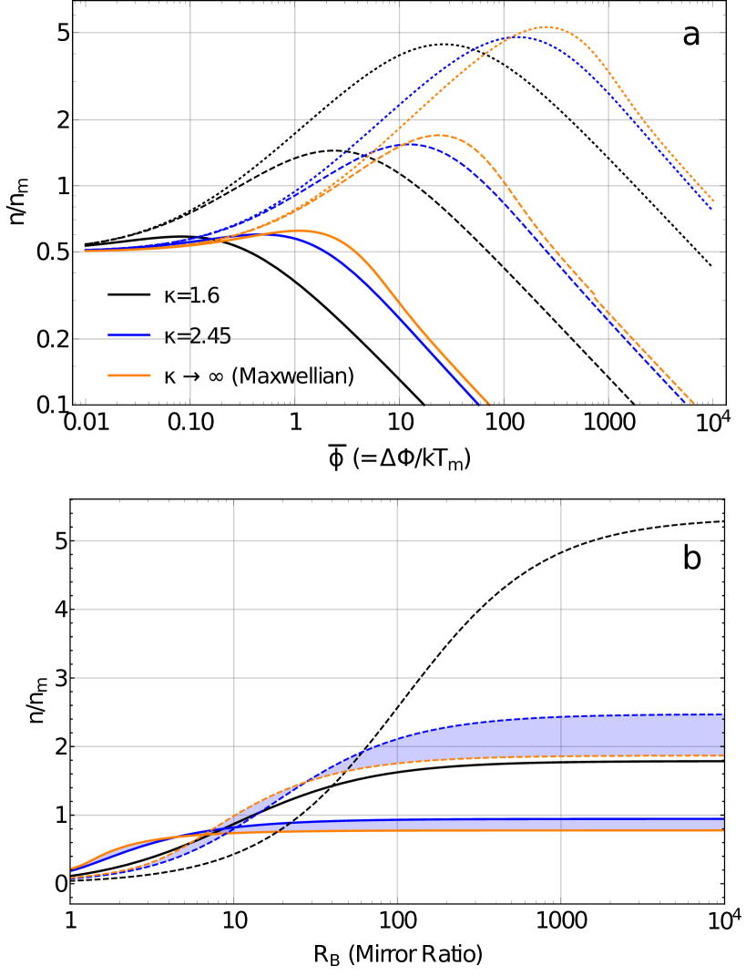
Figure 1: Number density–voltage (n-V) relationships in Equations (13) and (12). The ratio $n/n_{m}$ is plotted on the $y$ axis, where $n_{m}$ is magnetospheric source population density, and $n$ is the density at the altitude corresponding to mirror ratio $R_{B}$ and to the bottom of normalized potential drop $\overline{\phi}=\Delta\Phi/T_{m}$. (a) n-V relationships as a function of $\overline{\phi}$ for $R_{B}=$ 3 (solid lines), $R_{B}=$ 30 (dashed lines), and $R_{B}=$ 300 (dotted lines). (b) n-V relationships as a function of $R_{B}$ for $\overline{\phi}=$ 1 (solid lines) and $\overline{\phi}=$ 10 (dashed lines). In Figure 1b the region between the $\kappa=\kappa_{t}$ and $\kappa\rightarrow\infty$ curves is shaded.

Figure 1a shows the n-V relationships as a function of $\overline{\phi}$ for Maxwellian ($\kappa\rightarrow\infty$, orange lines), moderately nonthermal ($\kappa=\kappa_{t}$, blue lines), and extremely nonthermal ($\kappa=1.6$, blue lines) source populations. Mirror ratios of 3, 30, and 300 are respectively represented by solid, dashed, and dotted lines.

It is evident that $n/n_{m}\rightarrow 1/2$ in the limit $\overline{\phi}\rightarrow$ 0; this behavior is shown analytically for the Maxwellian n-V relation in the asymptotic expression (17). On the other hand $n/n_{m}\rightarrow 0$ for $\overline{\phi}\gg R_{B}$, as shown in the asymptotic expression (18).

The n-V relationships predict half the source density $n_{m}$ in the $\overline{\phi}\rightarrow$ 0 limit (i.e., no field-aligned potential) because only those particles in the magnetospheric source region having a parallel velocity component toward the ionosphere (defined as $v_{\parallel}>0$) are included in the range of integration used to obtain the n-V relationships; all others move away from the ionosphere and are ignored (Appendix A). This restriction on the range of integration is identically the reason that in the $\overline{\phi}\rightarrow$ 0 limit the J-V relations (1) and (6) and the J_E-V relationships (7)–(11) respectively predict nonzero current densities, or “thermal flows” (Theoretical Building Blocks, 2003), and nonzero energy fluxes. For instance, in this limit $j_{\parallel,M}=-en_{m}(T_{m}/2\pi m_{e})^{1/2}$. (See, e.g., Figure 3.8 in Theoretical Building Blocks, 2003.)

More generally, increasing $\overline{\phi}$ (i) increases the number of particles that have access to lower altitudes by increasing $v_{\parallel}$, which increases $n/n_{m}$ (the total volume under the distribution function), and (ii) compresses the distribution function in velocity space (see Inequality (16a)), which decreases $n/n_{m}$. On the other hand increasing $R_{B}$ while simultaneously conserving the first adiabatic invariant causes the distribution function to evolve toward an annular or “ring” distribution, such that (i) particles at large pitch angles ($v_{\perp}>v_{\parallel}$) in the source region are reflected at lower altitudes, which decreases $n/n_{m}$, and (ii) particles with small pitch angles ($v_{\parallel}>v_{\perp}$) in the source region, particularly those near the peak of the distribution near $v_{\parallel}=\sqrt{2e\Delta\Phi/m}$ also spread to larger pitch angles, increasing the total volume under the distribution function and thereby increasing $n/n_{m}$. The maximum values of $n/n_{m}$ in Figure 1a thus represent nontrivial interplay of these competing factors (see Equation 19).

Figure 1b shows as a function of $R_{B}$ the Maxwellian and kappa n-V relationships (12) and (13) normalized by source density $n_{m}$, for $\overline{\phi}=$ 1 (solid lines), $\overline{\phi}=$ 10 (dashed lines), and several values of $\kappa$. The magnetospheric source region corresponds to $R_{B}=1$. For a Maxwellian source population in the limit $R_{B}\rightarrow 1$, $n$ is given by the first term in the Maxwellian n-V relation (13). For a kappa source population in the limit $R_{B}\rightarrow 1$, $n$ approaches values similar to that approached by the Maxwellian curve. The topmost curve in Figure 1b shows that for $\overline{\phi}=10\ll R_{B}$ and $\kappa=1.6$, the density at lower altitudes increases by as much as a factor 5. More generally, $n/n_{m}\propto\sqrt{\overline{\phi}/(1-\frac{3}{2\kappa})}$ for $1\lesssim\overline{\phi}\ll R_{B}$. The shaded region between the $\kappa=\kappa_{t}$ and $\kappa\rightarrow\infty$ curves (blue and orange, respectively) in Figure 1b indicates that there is little difference, generally less than 30%, between the Maxwellian and kappa n-V relationships for $\kappa\gtrsim\kappa_{t}$ and equal $\overline{\phi}$. Asymptotic expressions for the Maxwellian n-V relation (12) are given in Appendix A.

2.2 Uncertainty of Distribution Moments

This study also relies on moments of measured electron distributions, including the number density $n$, field-aligned current density $j_{\parallel}=e\langle nv_{\parallel}\rangle$ and field-aligned energy flux $j_{E\parallel}=\frac{m}{2}\langle nv^{2}v_{\parallel}\rangle$. Estimation of the uncertainty of moments has typically involved generation of statistics of each moment via Monte Carlo simulation of $f(\mathbf{v})$ (e.g., Moore ., 1998). We alternatively use standard techniques of linearized uncertainty analysis to derive analytic expressions for the uncertainties of field-aligned current density and energy flux, respectively $\sigma_{j_{\parallel}}$ and $\sigma_{j_{E\parallel}}$, as functions of moments of $f(\mathbf{v})$ and moment covariances. (The uncertainty of number density $n$ is trivially $\sigma_{n}$.) Moment covariances are calculated following the methodology of Gershman . (2015). In Appendix B we present both these analytic expressions and a summary of the Gershman . (2015) methodology, which together enable the Monte Carlo simulations presented in sections 3.2 and 4.2.

3 Orbit 1607

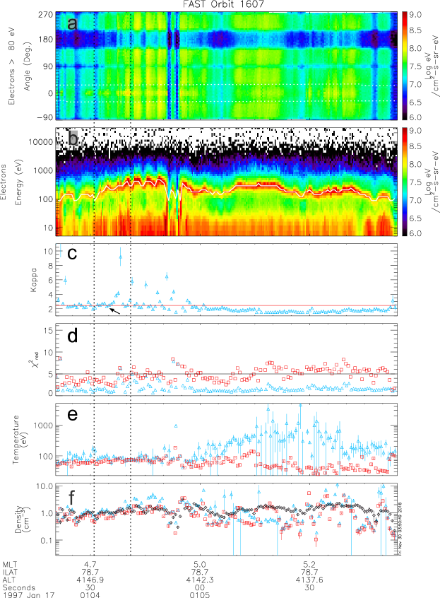
Figure 2: EESA observations of inverted V precipitation on Jan 17, 1997, and corresponding 2-D fit parameters. Parameters related to best-fit Maxwellian and kappa distributions are respectively indicated by red squares and blue triangles in panels c–f. (a) $>$80 eV electron pitch-angle distribution. The earthward portion of the loss cone (see text for definition) comprises the $\sim$60^∘ range of pitch angles between the dotted horizontal lines at $\sim$30^∘ and $\sim$-30^∘. (b) Average electron energy spectrum within the earthward loss cone. (c) $\kappa$ fit parameter for the best-fit kappa distribution. The red horizontal line indicates $\kappa=\kappa_{t}\simeq$ 2.45. The black arrow indicates the kappa value for fits shown in Figure 3. (d) Reduced chi-squared statistic $\chi^{2}_{\mathrm{red}}$ for each fit type. The black horizontal line indicates $\chi^{2}_{\mathrm{red}}=5$. (e) Best-fit temperatures. (f) Calculated density moments (black diamonds) and best-fit densities. Calculated densities are obtained as 2-D model-independent moments of the differential flux measured over pitch angles $|\theta|\leq$ 30^∘, from the energy of the channel immediately below the peak energy $E_{p}$ up to 5 keV. Resulting density moments and uncertainties (vertical black bars) are then multiplied by the ratio of the solid-angle ratio $1/(1-\cos 30^{\circ})\approx 7.46$. Uncertainties of best-fit parameters represent 90% confidence intervals obtained via Monte Carlo simulations with $N=$ 5,000 trials. EESA observations are integrated to obtain an effective sample period $T=0.63$ s.

3.1 Data Presentation

During an approximately 90-s interval on Jan 17, 1997, the FAST satellite observed inverted V electron precipitation over 80–600 eV (Figures 2a and 2b) and over $\sim$4.5–5.5 magnetic local time (MLT) in the Northern Hemisphere during low geomagnetic activity ($K_{p}=$ 0^-). Figure 2a shows that over much of this interval the distributions include both isotropic and trapped components, while the anti-earthward loss cone is relatively depleted. For instance over 01:05:10–01:05:15 UT the isotropic component is somewhat weak ($dJ_{E}/dE\lesssim 3\times 10^{7}$eV/cm²-s-sr-eV) and the trapped component is relatively more intense ($dJ_{E}/dE\gtrsim 10^{8}$eV/cm²-s-sr-eV).

Figure 2b gives the observed electron energy spectrogram averaged over observations at all pitch angles within the earthward loss cone. The loss cone is calculated from model geomagnetic field magnitudes at FAST and at the 100-km ionospheric footpoint, which are both obtained from International Geomagnetic Reference Field 11 (IGRF 11). For the period indicated between dashed lines (01:04:28–01:04:41 UT), which we will discuss momentarily, Figure 2b shows that the peak energy of monoenergetic electron precipitation varies between 80 eV and 500 eV.

We perform full 2-D fits to the portion of electron distributions that are observed within the earthward loss cone (horizontal dotted white lines in Figure 2a) and between the energy at which the distributions peak above 80 eV ($E_{p}$) up to the 30-keV limit of FAST electron electrostatic analyzers (EESAs) (Carlson ., 2001). To obtain these fits, we first form a 1-D differential number flux distribution by averaging the counts within each EESA energy-angle bin over the range of angles within the earthward portion of the loss cone, after which 1-D fits of the resulting average differential number flux spectrum are performed using the model differential number flux $J=\frac{2E}{m^{2}}f\left(E-E_{p}\right)$, with $f\left(E-E_{p}\right)$ either a 1-D Maxwellian or 1-D kappa distribution. The resulting 1-D best-fit parameters then serve as initial estimates for 2-D fits of the observed differential energy flux spectrum, over the previously described range of pitch angles and energies, using model differential energy flux $dJ_{E}/dE=\frac{2E^{2}}{m^{2}}f\left(E-E_{p}\right)$. Both 1-D and 2-D distribution fits are performed using Levenberg-Marquardt weighted least-squares minimization via the publicly available Interactive Data Language MPFIT library (http://cow.physics.wisc.edu/ craigm/idl/fitting.html).

The most probable fit parameters and 90% confidence intervals are then obtained by following a procedure similar to those recently employed by Kaeppler . (2014) and Ogasawara . (2017): for each time and each type of distribution, we fit $N=$ 5,000 Monte Carlo simulated 2-D distributions by adding to each best-fit distribution a normal random number $Z\sim\mathcal{N}(0,1)$ that is multiplied by the counting uncertainty (section 15.6 in Press ., 2007) in units of differential energy flux. For the simulated kappa distribution fits we also select a uniform random number $K\sim U(\kappa_{\textrm{min}},35)$ as an initial guess for $\kappa$.

For each fit parameter we then form a histogram from the resulting 5,000 Monte Carlo values. The value at which the histogram peaks is taken to be the most probable fit parameter. We then use a simple algorithm that increases the size of a window centered on the most probable fit parameter until 4,500 (90%) of the parameter values are included in the window.

Reported parameters are $\kappa$ (Figure 2c) for the kappa distribution, and temperature (Figure 2e) and density (Figure 2f) for both Maxwellian and kappa distribution fits. For each most probable fit parameter the 90% confidence interval is indicated by a vertical bar. In many instances the upper and lower limits of the 90% confidence interval are very near the most probable fit parameter value. For example, for over 92% of the most probable $\kappa$ parameters in Figure 2c the upper and lower limit of the 90% confidence interval is within 10% of the most probable $\kappa$ parameter itself.

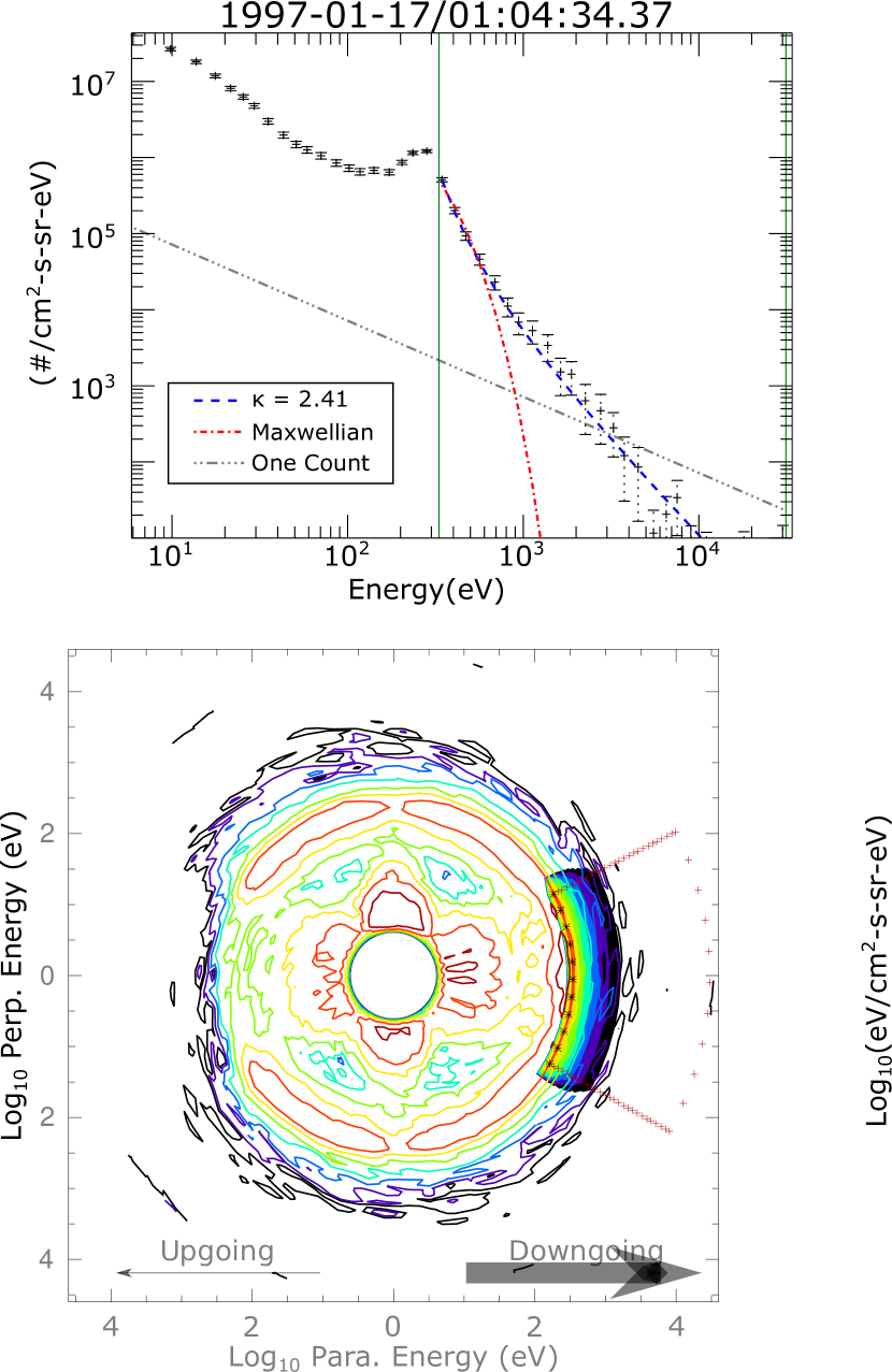
Figure 3: Electron spectra observed at 01:04:34.37–01:04:35.00 UT. (a) 1-D differential number flux spectrum (black crosses) obtained by averaging differential number flux spectra over all pitch angles within the earthward loss cone, with best-fit Maxwellian and kappa distributions overlaid (red dash-dotted line and blue dashed line, respectively). The uncertainty of each observed differential number flux is calculated by conversion of the electron count uncertainty $\sqrt{N}$ to units of differential number flux. (b) Best-fit 2-D kappa distribution (solid contours) with the observed 2-D differential energy flux spectrum overlaid (contour lines). The color bar at right shows the differential energy flux of each contour. For each pitch angle black asterisks indicate the peak energy $E_{p}=315$ eV, and red plus signs outline the range of energies and pitch angles used to perform the 2-D fit.

Figure 3 shows example 1-D (Figure 3a) and 2-D (Figure 3b) distribution fits to electron observations during 01:04:34.37–01:04:35.00 UT, indicated by the black arrow in Figure 2c. The observed distribution in Figure3a (black plus signs and error bars) is much better described by the best-fit kappa distribution (blue dashed line) than by the best-fit Maxwellian distribution (red dash-dotted line). The overall better description that the kappa distribution fits yield for observations throughout the entire 90-s interval is indicated in Figure 2d, which shows values of the reduced chi-squared statistic

$$\chi_{\mathrm{red}}^{2}=\sum\limits_{i}^{N}\frac{1}{F}\frac{\left(Y_{i}(x)-y_{i}(x)\right)^{2}}{w_{i}^{2}}$$ (14)

for 2-D fits using either a kappa distribution (blue triangles) or a Maxwellian distribution (red squares). In this expression $i$ indexes each pitch-angle and energy bin used in the fitting procedure, $Y_{i}$ is the observed differential energy flux, $y_{i}$ is the differential energy flux of the original best-fit 2-D model distribution, $w_{i}$ is the uncertainty due to counting statistics, and $F$ is the degrees of freedom, or the total number of pitch angle–energy bins $N$ minus the number of free model parameters. The difference is most pronounced after approximately 01:05:00 UT, corresponding to the interval during which $\kappa_{\textrm{min}}<\kappa\lesssim$ 2 in Figure 2c.

Figure 2e shows that over approximately the first half of the 90-s interval, $T=$ 30–200 ev for both Maxwellian and kappa distribution fits. Comparison with statistical plasma sheet temperatures reported by Kletzing . (2003) (their Figure 4) indicates that these temperatures are within typical ranges. During the latter half of the interval the most probable kappa temperatures tend to be much higher ($\sim$100–2000 eV) than during the first half, while corresponding Maxwellian temperatures remain low (20–100 eV). The kappa “core temperatures” (Nicholls ., 2012) $T_{c}=T(1-\frac{3}{2\kappa})$ (not shown) during the latter half are nonetheless within several eV of Maxwellian temperatures.

Figure 2f shows that relative to the calculated densities, the best-fit densities for Maxwellian and kappa distributions are generally within factors of two to five. For calculated densities the corresponding uncertainties (vertical black bars) are obtained using analytic expressions for moment uncertainties related to counting statistics for an arbitrary distribution function (Gershman ., 2015). These uncertainties are generally less than 10% of the calculated density.

3.2 Inference of magnetospheric source parameters

We now demonstrate how the observed electron distributions may indicate the properties of the magnetospheric source region. This is performed via comparison of the predictions of moment-voltage relationships (1) and (6)–(13) with experimental moment-voltage relationships derived from model-independent fluid moments of the electron distributions observed during the delineated interval between dashed lines in Figure 2, 01:04:31–01:04:41 UT. We have selected this interval because it is associated with the largest variation in the inferred potential during the entire 90-s period.

The J-V and J_E-V relationships are formed by first determining the potential drop $\Delta\Phi$ (solid white line, Figure 2b) at each time, which is taken to be the peak electron energy $E_{p}$. (There is no potential drop below FAST during this interval, which would otherwise be indicated by the presence of upgoing ion beams; see, e.g., Elphic ., 1998; Hatch ., 2018.) We define the peak energy $E_{p}$ as the energy of the EESA channel above which the observed differential flux spectrum exhibits exponential or power-law decay (Kaeppler ., 2014; Ogasawara ., 2017), within the earthward loss cone. We then calculate the parallel electron current density $j_{\parallel,i}$ and energy flux $j_{E\parallel,i}$ of the observed electron distribution, using measurements from the peak energy $E_{p}$ up to 5 keV and the range of angles within the earthward loss cone. The upper bound of the energy integration range is limited to 5 keV because statistics of particles above this energy are poor and contribute almost exclusively to the uncertainty of these moments. These two moments are mapped to the ionosphere at 100 km using IGRF 11 (denoted by the subscript $i$).

The n-V relationship is also formed from the inferred potential drop $\Delta\Phi$ and from the calculated number density $n$, but unlike the fluxes $j_{\parallel,i}$ and $j_{E\parallel,i}$, $n$ is not a flux and is not straightforward to map to the ionosphere. We therefore must form a “local” (i.e., unmapped) n-V relationship and obtain $n$ via integration over the same range of energies that are used to calculate $j_{\parallel,i}$ and $j_{E\parallel,i}$ (from $E_{p}$ up to 5 keV), but over a modified pitch angle range, which in a local treatment should be the full 180^∘ range of earthward pitch angles. However, inspection of the delineated interval in Figure 2a indicates the presence of a prominent trapped population at pitch angles $|\theta|\gtrsim$ 40^∘ (e.g., at 01:04:37 UT) that should not be included in the calculation of $n$. We therefore integrate over a 60^∘ range of angles that is centered on the earthward loss cone and multiply both the calculated densities and their uncertainties by the solid-angle ratio $1/(1-\cos 30^{\circ})\approx 7.46$ to compensate for the exclusion of observations over pitch angles $|\theta|>$ 30^∘. This multiplication assumes the primary electron distribution is isotropic outside the loss cone.

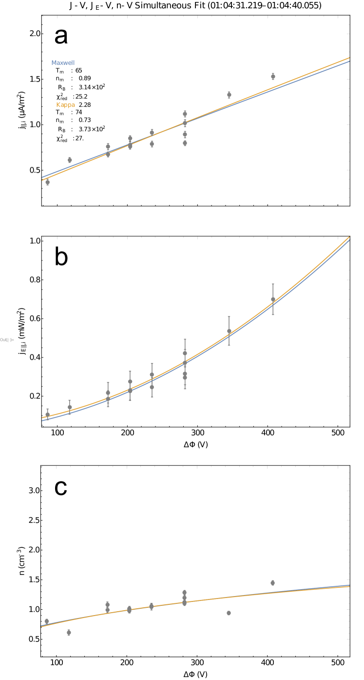
Figure 4: J-V, J_E-V, and n-V relationships inferred from electron observations during the interval 01:04:28–01:04:41 UT in Figure 2, together with best-fit Maxwellian (solid blue lines) and kappa (solid orange lines) moment-voltage relationships obtained by simultaneously fitting all three experimentally inferred moment-voltage relationships. (a) J-V relationship. (b) J_E-V relationship. (c) n-V relationship. Given values of the inferred potential drop $\Delta\Phi$ occur multiple times within the sample interval, causing the experimental data to be multi-valued. Calculated current densities and energy fluxes (bullets) as well as their uncertainties (1$\sigma$) are mapped to the ionosphere at 100 km as described in the text. Calculated number densities are not mapped to the ionosphere. Moment uncertainties are obtained as analytic moments of observed electron distributions, as described in Appendix B. The $\chi_{\mathrm{red}}^{2}$ values indicated in Figure 4a are the sum of the $\chi_{\mathrm{red}}^{2}$ value corresponding to each moment-voltage relationship.

The experimental J-V, J_E-V, and n-V relationships are shown in Figures 4a–c. Also shown are the results of simultaneously fitting all three of these relationships with the corresponding Maxwellian and kappa moment-voltage relationships (1)–(13) using NonlinearModelFit in the Mathematica^® (v11.3) programming language. The best-fit Maxwellian (blue lines) and kappa (orange lines) fits correspond to $\chi^{2}_{\mathrm{red}}=$ 25.2 and $\chi^{2}_{\mathrm{red}}=$ 27, respectively, where these two $\chi^{2}_{\mathrm{red}}$ values are the sum of the three $\chi^{2}_{\mathrm{red}}$ corresponding to each type of moment-voltage relation.

We obtain these fits by drawing from random variables $N\sim U($0.05 cm^-3,1.5 cm${}^{-3})$ and $R\sim U(5,10^{4})$ to initialize $n_{m}$ and $R_{B}$ in each moment-voltage relationship. For the kappa moment-voltage relationships we must also draw from a random variable to initialize the $\kappa$ parameter. To accomplish this we randomly choose a degree of correlated motion $W\sim U(0.05,0.85)$ (see Equation 3), from which we obtain an initial kappa value $K\sim\kappa_{\textrm{min}}/W$. The lower and upper bounds of the uniformly random degree of correlation $W$, $\rho=0.05$ and $\rho=0.85$, respectivly correspond to $\kappa=30$ and $\kappa=1.76$.

For both types of fits the parameter $T_{m}$ is held fixed. For the fits involving the Maxwellian moment-voltage relationships the value of $T_{m}$ is set equal to the median (65 eV) of the best-fit Maxwellian distribution temperatures (red boxes in Figure 2e) during the marked interval. For the fits involving the kappa moment-voltage relationships the value of $T_{m}$ is set equal to the median (74 eV) of the best-fit kappa distribution temperatures (blue triangles in Figure 2e). Additionally, because the experimental $n$ values in Figure 4c are not mapped to the ionosphere, the $R_{B}$ parameter in the n-V relationships (12)–(13) must be reduced by a factor $R_{B,\textrm{FAST}}=\frac{B_{i}}{B_{\textrm{FAST}}}\approx 4$ when fitting the experimental n-V relationship.

Similar to the process described at the beginning of this section for Monte Carlo simulation of 2-D distribution fits, to determine the range of parameters that may describe the observed moment-voltage relationships we perform fits to $N=$ 2,000 Monte Carlo simulated moment-voltage relationships for each type of J-V, J_E-V, and n-V relationship, either Maxwellian or kappa. For each iteration, we add to each of the inferred potential drop values a uniform random number $X\sim\mathcal{N}(0,\Delta E_{p})$, where the value in the second argument is the uncertainty of the electron peak energy, which arises from the EESA energy channel spacing. We insert these synthetic potential drop values into the best-fit J-V, J_E-V,and n-V relationships and add to each of these theoretical moment predictions a normal random number $Z\sim\mathcal{N}(0,1)$ multiplied by the uncertainty of the corresponding current density, energy flux, or number density measurements. We then draw from the random variables $N$, $R$, and $K$, which are as described above, to initialize $n_{m}$, $R_{B}$, and $\kappa$, respectively. We then perform the fit.

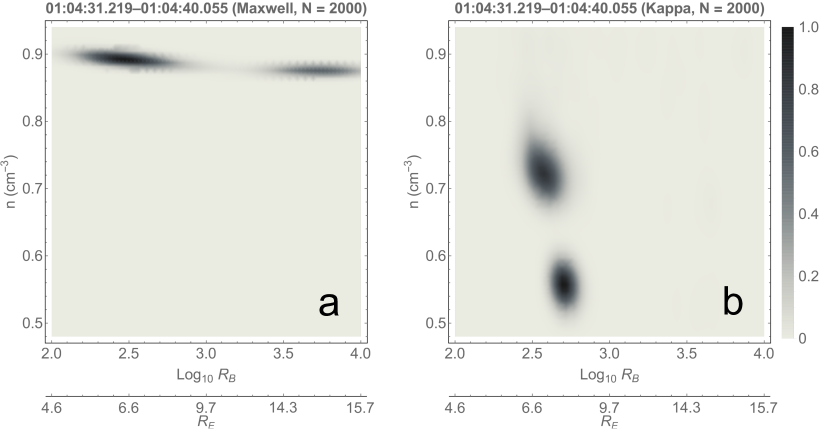
Figure 5: (a) Joint distribution of density $n_{m}$ and mirror ratio $R_{B}$ for Maxwellian fits of $N=$ 2,000 Monte Carlo simulated J-V, J_E-V, and n-V relationships (1), (7), and (12). (b) Same as Figure 5a, except that fits are performed using the kappa J-V, J_E-V, n-V relationships (6), (11), and (13). In both panels the $R_{B}$ axis is logarithmic and the secondary axis shows the approximate source height $h$ in Earth radii. The gray scale indicates the distribution height in units such that the peak value of each distribution is 1.0.

The resulting joint distributions of $n_{m}$ and $R_{B}$ are shown in Figures 5a and 5b for the Maxwellian and kappa moment-voltage relationships, respectively. The Maxwellian moment-voltage relationships predict two different solution regimes: the first corresponds to $n_{m}=$ 0.88–0.90 cm^-3 and $R_{B}=$ 200–500; the second corresponds to $n_{m}=$ 0.87–0.88 cm^-3 and $R_{B}=$ 3,200–7,500. The secondary axis indicates the approximate source altitudes $h=$5.7–7.7 $R_{E}$ and $h=$14–15.5 $R_{E}$, respectively, where $R_{E}$ indicates the radius of Earth. The kappa moment-voltage relationships also show two different solution regimes: the first corresponds to $n_{m}=$ 0.70–0.79 cm^-3, $R_{B}=$ 300—510 ($h=$6.4–7.7 $R_{E}$), and $\kappa=$ 2.2–2.8; the second corresponds to $n_{m}=$ 0.55–0.56 cm^-3, $R_{B}=$ 300–500 ($h=$6.4–7.6 $R_{E}$), and $\kappa\leq$ 1.8.

The $\chi^{2}_{\mathrm{red}}$ value for the kappa fits in Figure 4 is 7% greater than the $\chi^{2}_{\mathrm{red}}$ value for the Maxwellian fits. It therefore seems impossible to determine the correct solution regime solely on the basis of information in Figures 4 and 5. However, only the first kappa solution regime is consistent with the range $\kappa=$ 2–9 that arises from direct 2-D distribution fits during the 10-s delineated period in Figure 2c.

We have also performed $N=6,000$ Monte Carlo simulations using only the inferred J-V relationship (Figure 4a) and either the the Maxwellian J-V relation (1) or the kappa J-V relation (6). From the Maxwellian J-V relation we obtain solutions corresponding to $n_{m}=$ 0.88–0.90 cm^-3 and $R_{B}\geq$ 680 ($h\geq$8.5 $R_{E}$). From the kappa J-V relation (6) we obtain solutions corresponding to $n_{m}=$ 0.68–0.84 cm^-3 and $R_{B}\geq$ 2,100 ($h\geq$12.8 $R_{E}$) for $\kappa=$ 2.2–2.8. Thus for this case study and an assumed Maxwellian or kappa source population, the source altitude lower bound is relatively greater when only the J-V relationship is used.

4 Orbit 4682

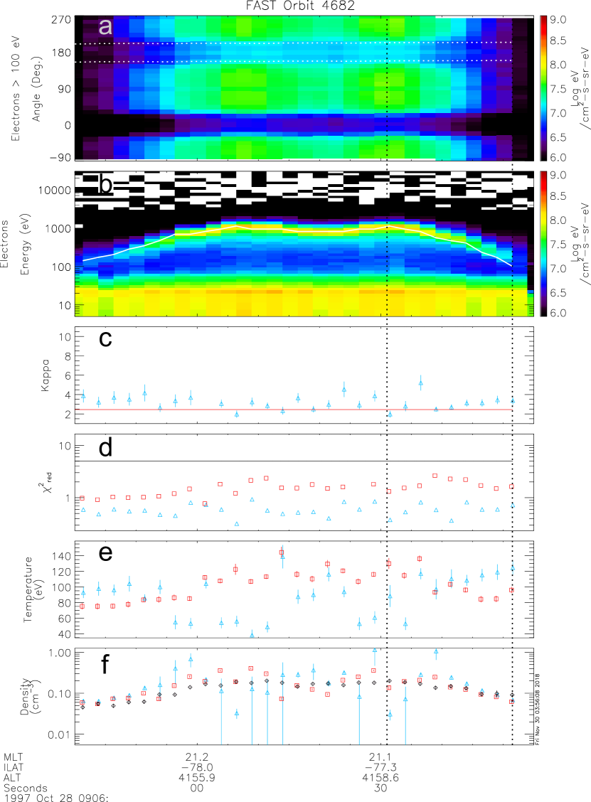
Figure 6: EESA observations of inverted V precipitation on Oct 28, 1997 and corresponding 2-D fit parameters, in the same format as Figure 2. (a) $>$100 eV electron pitch-angle distribution. The earthward portion of the loss cone comprises the range of pitch angles between dotted horizontal lines at $\sim$150^∘ and $\sim$210^∘. (b) Average electron energy spectrum within the earthward loss cone. (c) $\kappa$ fit parameter for the best-fit kappa distribution. (d) Reduced chi-squared statistic $\chi^{2}_{\mathrm{red}}$ for each fit type. (e) Best-fit temperatures. (f) Calculated and best-fit densities. Calculated densities are also obtained as model-independent moments via integration over from the energy of the channel immediately below $E_{p}$ up to 5 keV, and over all pitch angles $|\theta|>$ 150^∘. Uncertainties of calculated densities and best-fit density and temperature parameters are obtained as described in the Figure 2 caption. EESA observations during this interval have a sample period $T=2.5$ s.

4.1 Data Presentation

During a 75-s interval on Oct 28, 1997, the FAST satellite observed inverted V electron precipitation (Figures 6a and 6b) at $\sim$21 MLT and -78^∘ invariant latitude in the Southern Hemisphere during moderately low geomagnetic activity ($K_{p}=$ 2). The pitch-angle spectrogram in Figure 6a shows that precipitation within the earthward loss cone (range of pitch angles between horizontal dotted white lines in Figure 6a) is weak ($dJ_{E}/dE\lesssim 5\times 10^{7}$eV/cm²-s-sr-eV), while trapped electrons over 30${}^{\circ}\lesssim|\theta|\lesssim$ 150^∘ are relatively more intense. Over the entire 75-s interval as well as over the $\sim$20-s period between dashed lines, 09:06:31–09:06:51.5 UT, Figure 6b and c respectively show $E_{p}=$ 100–1200 eV and $\kappa\approx$ 2–5. Figure 6d shows that best-fit Maxwellian $\chi^{2}_{\mathrm{red}}$ values are generally twice or more those of best-fit kappa $\chi^{2}_{\mathrm{red}}$ values.

Best-fit temperatures shown in Figure 6e indicate that over the entire interval $T=$ 75–130 ev for Maxwellian distribution fits, while $T=$ 35–145 ev for kappa distribution fits. As with temperatures in Figure 2e, these ranges of temperatures are within the typical range for plasma sheet electrons.

Densities calculated directly from observed electron distributions in Figure 6f (black diamonds) are within the range 0.01–0.5 cm^-3 that is typically observed in the distant plasma sheet (Kletzing ., 2003; Theoretical Building Blocks, 2003). Most probable Maxwellian and kappa fit densities in Figure 6f tend to be with factors of 2 of the calculated densities. Similar to the density moments and uncertainties calculated in the previous section, we calculate the density over all energies from $E_{p}$ up to 5 keV and over all earthward pitch angles in the Southern Hemisphere, $|\theta|>$ 150^∘. We multiply calculated densities and density uncertainties by the solid-angle ratio $1/(1-\cos 30^{\circ})\approx 7.46$ to compensate for the exclusion of primary electrons over the range of downgoing pitch angles dominated by trapped electrons ($90^{\circ}<\theta<$ 150^∘ and $-$150${}^{\circ}<\theta<-90^{\circ}$).

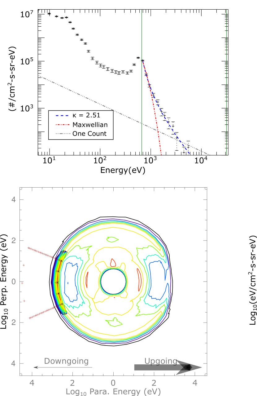
Figure 7: Electron spectra observed at 09:06:38.931–09:06:41.437 UT. The layout is the same as that of Figure 3. (a) 1-D differential number flux spectrum (black crosses) obtained by averaging all differential number flux spectra over all pitch angles within the earthward loss cone, with best-fit Maxwellian and kappa distributions overlaid (red dash-dotted line and blue dashed line, respectively). (b) Best-fit 2-D kappa distribution (solid contours) with the observed 2-D differential energy flux spectrum overlaid (contour lines). For each pitch angle black asterisks indicate the peak energy $E_{p}=560$ eV, and red plus signs outline the range of energies and pitch angles used to perform the 2-D fit.

Figure 7 shows an example of the electron distributions observed during the delineated period (09:06:31–09:06:51.5 UT), in the same layout as Figure 3. As in Figure 3, the best-fit kappa distribution (blue dashed line) successfully describes the suprathermal tail, and is a better fit than the Maxwellian distribution (red dash-dotted line) as reflected in the $\chi^{2}_{\mathrm{red}}$ values, respectively 0.56 and 2.57 (also Figure 6d).

4.2 Inference of magnetospheric source parameters

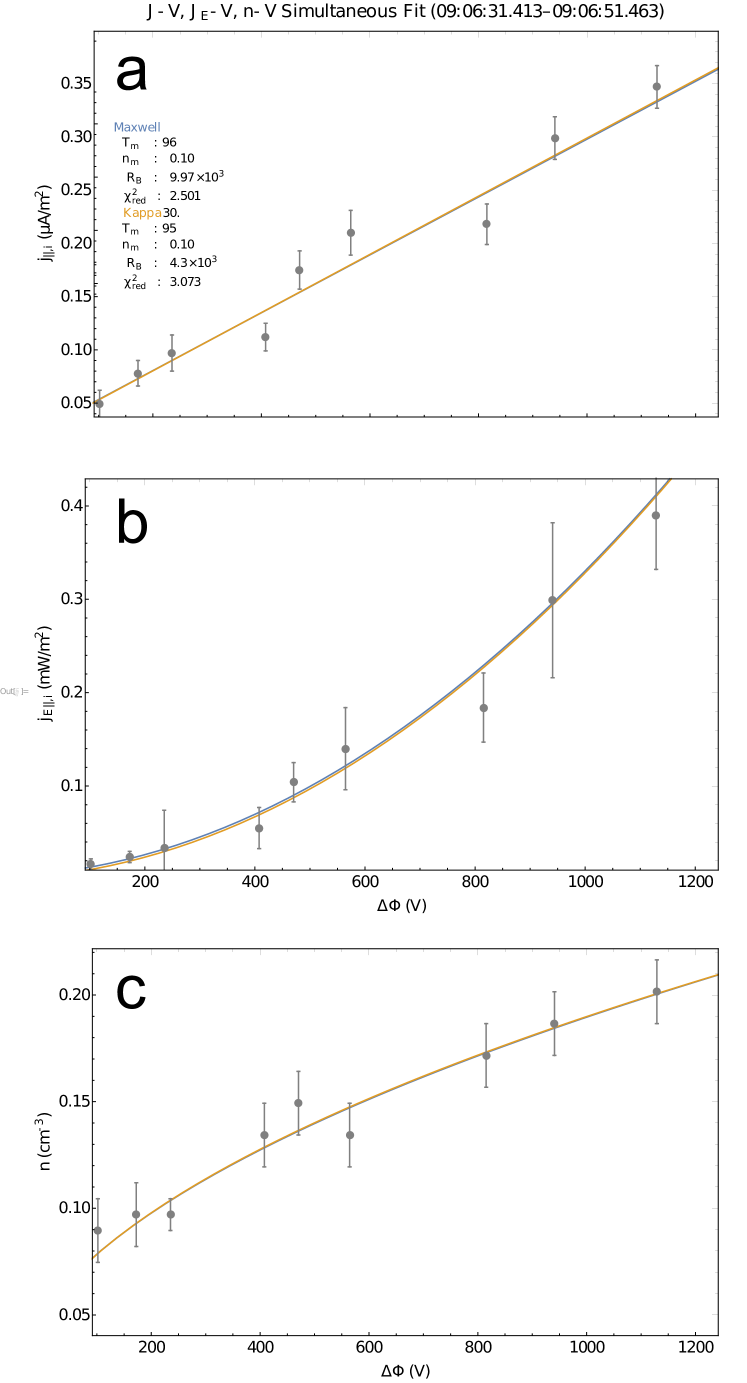
Figure 8: J-V, J_E-V, and n-V relationships inferred from electron observations during the interval 09:06:31–09:06:51.5 UT in Figure 6, together with best-fit Maxwellian (solid blue lines) and kappa (solid orange lines) moment-voltage relationships obtained by simultaneously fitting all three experimentally inferred moment-voltage relationships. The format is the same as that of Figure 4. (a) J-V relationship. (b) J_E-V relationship. (c) n-V relationship. Calculated current densities and energy fluxes (black plus signs) as well as their uncertainties (1$\sigma$) are mapped to the ionosphere at 100 km as described in section 3.2. Calculated number densities are not mapped to the ionosphere. Moment uncertainties are obtained as analytic moments of observed electron distributions (Appendix B). The $\chi_{\mathrm{red}}^{2}$ values indicated in Figure 8a are the sum of the $\chi_{\mathrm{red}}^{2}$ values corresponding to each moment-voltage relationship.

Using the Monte Carlo simulation process described in section 3.2, we now determine the range of parameters that may describe the observed moment-voltage relationships during the 20-s period shown between dashed lines in Figure 6 assuming each type of magnetospheric source population, either Maxwellian or kappa. We select this period because the inferred potential drop (solid white line in Figure 6b) decreases by roughly an order of magnitude, from $\sim$1150 eV to $\sim$150 eV.

The experimental J-V, J_E-V, and n-V relationships are shown in Figures 8a–c. Also shown are the results of simultaneously fitting all three of these relationships with the corresponding Maxwellian and kappa moment-voltage relationships (1), (6)–(13). Best-fit Maxwellian (blue lines) and kappa (orange lines) fits respectively correspond to $\chi^{2}_{\mathrm{red}}=$ 2.5 and $\chi^{2}_{\mathrm{red}}=$ 3.1. As in section 3.2, we obtain these fits by drawing from random variables $N\sim U($0.01 cm^-3,0.5 cm^-3), $R\sim U(5,10^{4}),$ and $K\sim\kappa_{\textrm{min}}/W$ to initialize $n_{m}$, $R_{B}$, and $\kappa$ in each moment-voltage relationship. (The random variable $K$ is only used in the kappa moment-voltage relationships.) For both types of fits the parameter $T_{m}$ is held fixed. For the fits involving the Maxwellian moment-voltage relationships the value of $T_{m}$ is set equal to the median $T=$ 96 eV of the best-fit Maxwellian distribution temperatures (red boxes in Figure 6e) during the marked interval. For the fits involving the kappa moment-voltage relationships the value of $T_{m}$ is set equal to the median $T=$ 95 eV of the best-fit kappa distribution temperatures (blue triangles in Figure 6e).

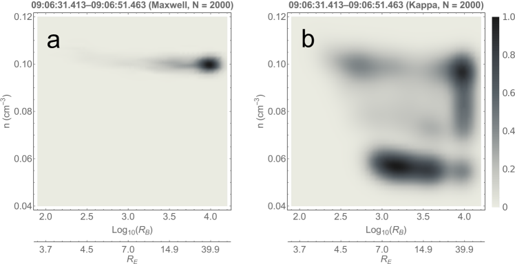
Figure 9: (a) Joint distribution of density $n_{m}$ and mirror ratio $R_{B}$ for Maxwellian fits of $N=$ 2,000 Monte Carlo simulated J-V, J_E-V, and n-V relationships (1), (7), and (12). (b) Same as Figure 9a, except that fits are performed using the kappa J-V, J_E-V, n-V relationships (6), (11), and (13). In both panels the $R_{B}$ axis is logarithmic and the secondary axis shows the approximate source height $h$. The gray scale indicates the distribution height in units such that the peak value of each distribution is 1.0.

The resulting joint distributions of $n_{m}$ and $R_{B}$ is shown in Figures 9a and 9b for the Maxwellian and kappa moment-voltage relationships, respectively, in a layout identical to that of Figure 5. The Maxwellian moment-voltage relationships predict $n_{m}=$ 0.097–0.103 cm^-3 and $R_{B}\geq$1,400 ($h\geq$ 8.1 $R_{E}$). The kappa moment-voltage relationships show several different solution regimes, all of which correspond to $R_{B}\gtrsim$ 370 ($h\gtrsim$ 4.6 $R_{E}$) and $n_{m}=$ 0.055–0.10 cm^-3: the first overlaps with the Maxwellian solution regime in Figure 9a, and corresponds to $n_{m}=$ 0.096–0.0102 cm^-3, $R_{B}\geq$ 370 ($h\geq 4.6$), and $\kappa>10$; the second corresponds to $n_{m}=$ 0.072–0.094 cm^-3, $R_{B}\gtrsim$ 700 ($h\gtrsim 5.7$), and 2 $\leq\kappa\geq$ 10; the third corresponds to $n_{m}=$ 0.054–0.059 cm^-3, $R_{B}\gtrsim$ 10$~{}3$ ($h\gtrsim 6.8$), and $\kappa<$ 2.

The $\chi^{2}_{\mathrm{red}}$ value for the kappa fits in Figure 8 is $\sim$24% greater than the $\chi^{2}_{\mathrm{red}}$ value for the Maxwellian fits. As with results in the previous section, information in Figures 8 and 9 seems insufficient to determine the correct solution regime. However, only the second kappa solution regime is consistent with the direct 2-D distribution fits during the 20-s delineated period in Figure 6.

As in section 3.2 we have performed $N=6,000$ Monte Carlo simulations using only the inferred J-V relationship (Figure 8a) and either the the Maxwellian J-V relation or the kappa J-V relation. From the Maxwellian J-V relation the resulting solutions correspond to $n_{m}=$ 0.097–0.106 cm^-3 and $R_{B}\geq$ 1,900 ($h\geq$10 $R_{E}$). From the kappa J-V relation (6) we obtain solutions corresponding to $n_{m}=$ 0.071–0.093 cm^-3 and $R_{B}\geq$ 1,500 ($h\geq$8.6 $R_{E}$) for $\kappa=$ 2–10. Similar to results in section 3.2, the source altitude lower bound is relatively greater when only the J-V relationship is used.

5 Discussion and Summary

Table 1: Most likely magnetospheric source parameters

	Source Type	Temperaturea	Density	$R_{B}$	$h$	$\kappa$
		(eV)	(cm-3)		($R_{E}$)
Orbit 1607	Maxwellian	65	0.87–0.9	220–6,400	5.8–15
	Kappa	74	0.70–0.79	300–510	6.4–7.7	2.2–2.8
Orbit 4682	Maxwellian	96	0.097–0.103	$\geq$1400	$\geq$8.1
	Kappa	95	0.071–0.091	$\geq$720	$\geq$5.9	2–6
aFixed.

For the two case studies that we have presented we assume either Maxwellian or kappa source populations when fitting the observed J-V, J_E-V, and n-V relationships, which results in $\chi^{2}_{\mathrm{red}}$ values that differ by a few to several percent (see Figures 4 and 8). Such differences indicate that the moment-voltage relationships themselves are insufficient to determine the source region properties. We identify the most likely ranges of source densities and altitudes in each case study by requiring that these parameters correspond to the range of $\kappa$ values estimated from direct 2-D fits of observed electron distributions.

Table 1 summarizes the ranges of most likely source parameters for both case studies. As stated in previous sections, the estimated temperatures and densities are within or near the typical ranges expected on the basis of surveys of the plasma sheet. The combined range of $\kappa$ values estimated for each orbit, $\kappa=$ 2–6, are also within the ranges indicated by in situ plasma sheet surveys (Christon ., 1989, 1991; Kletzing ., 2003; Stepanova  Antonova, 2015).

The estimated ranges of source altitudes for these two case studies, $h=$ 6.4–7.7 for Orbit 1607 observations and $h\geq$ 5.9 $R_{E}$ for Orbit 4682 observations, are above the typically quoted range of altitudes $\sim$1.5–3 $R_{E}$ for the auroral acceleration region (Mozer  Hull, 2001; Morooka ., 2004; Marklund ., 2011). Results from previous studies (Wygant, 2002; Li ., 2014) indicate that such “high-altitude acceleration” scenarios often involve Alfvén wave-particle interactions, and Andersson . (2002) have shown that the signatures of these interactions at high altitudes may appear monoenergetic.

There are three primary limitations of this study. First, verification of the results shown in Table 1 requires conjunctive observations along similar field lines from FAST in the acceleration region and from another spacecraft in the source region; unfortunately the latter are not available during the intervals shown in Figures 2 and 6. Second, related to the previous point, the clear monoenergetic peaks in Figures 2b and 6b suggest that the potential structures above FAST are stationary relative to the transit time of plasma sheet electrons. We nevertheless cannot directly verify our assumption that quasistatic magnetospheric processes and monotonic potential structures are the cause of the electron precipitation shown in Figures 2a–b and Figures 6a–b. Third, the moment-voltage relationships (1) and (6)–(13) assume that the magnetospheric source population is isotropic.

Studies performed by Hull . (2010) and Marklund . (2011) have shown that potential structures are generally neither quasistatic nor monotonic, and Hatch . (2018) present statistics suggesting that electron distributions may be modified in the vicinity of the AAR. These studies indicate that our assumptions of stationarity, non-variability of source parameters along the mapped satellite track, and adiabatic transport from the source region to the ionosphere are not always true, and some evidence of violation of our assumptions appears in, for example, the experimental J-V relation (top panel) in Figure 4: For some data points neither the Maxwellian nor the kappa J-V relation is within 2–3$\sigma$. Such differences could suggest that the errors associated with our assumptions are larger than that associated with moment uncertainty and counting statistics.

Concerning the third limitation, magnetospheric source populations are not necessarily isotropic, and previous studies (Marghitu ., 2006; Forsyth ., 2012) have shown how the observed degree of anisotropy of electron precipitation may in fact be used to estimate the source altitude. While outside the scope of the present study, relaxing the assumption of isotropy and adapting the source altitude estimation techniques presented by these previous studies are natural future extensions of the techniques we have developed for the two case studies presented above.

Regardless of the particular values or ranges of parameters that we have identified, these case studies nevertheless demonstrate how the non-Maxwellian nature of an electron source population may be embedded in the observed moment-voltage relationships, requiring modification of both the inferred source density and mirror ratio. From this standpoint the degree to which a source population departs from thermal equilibrium, as indicated by the $\kappa$ parameter in this study, is as fundamental a plasma property as density or temperature.

A relatively small number of studies, such as those of Shiokawa . (1990); Lu . (1991); Morooka . (2004); Dombeck . (2013), has compared various forms of the Knight relation (1) to observations. To our knowledge, however, no study besides the present has used the moment-voltage relationships (1) and (6)–(13) that are predicted by Liouville’s theorem, or any subset thereof, to infer the properties of the magnetospheric source region on the basis of observations at lower altitudes.

In summary, in this study we have (i) derived the two previously unpublished n-V relationships (12) and (13); (ii) inferred the properties of magnetospheric source populations in two case studies based on simultaneous fitting of the three experimental moment-voltage relationships with corresponding theoretical moment-voltage relationships (1), (6)–(13), moment uncertainties, and direct 2-D fits of observed precipitating electron distributions; (iii) demonstrated that knowledge of the degree to which monoenergetic precipitation departs from Maxwellian form, which we parameterize via the $\kappa$ index, is required to determine the most likely set of magnetospheric source parameters.

Appendix A Theory of collisionless transport through a field-aligned monotonic potential structure

Here we review the theory that yields the J-V, J_E-V, and n-V relationships (1) and (6)–(13). The development is intended to be brief since several more elaborate developments have been given elsewhere (e.g., references in the Introduction).

Assuming a gyrotropic, collisionless magnetospheric source population, an electron distribution function $f(v_{\parallel},v_{\perp})$ can be written in terms of total energy and the first adiabatic invariant:

$$\begin{split}E&=\frac{m_{e}}{2}(v_{\parallel}^{2}+v_{\perp}^{2})+\Pi(B);\end{split}$$ (15a)

$$\begin{split}\mu&=\frac{m_{e}v_{\perp}^{2}}{2B(s)}.\end{split}$$ (15b)

In these expressions $v_{\parallel}$ and $v_{\perp}$ are parallel and perpendicular velocity, $\Pi(B)$ is the distribution of potential energy along the field line, $B(s)$ is magnetic field strength, and $s$ is a one-to-one function of $B$ that measures the distance along a magnetic field line from the magnetospheric source region toward the ionosphere. We denote the magnetic field strength at the source $B_{m}\equiv B(s_{0})$ and assume $\Pi(B_{m})=0$. Thus the initial total energy is $E_{0}=\frac{m_{e}}{2}(v_{\parallel,0}^{2}+v_{\perp,0}^{2})$. From Equations (15) we then have $v_{\parallel,0}^{2}=v_{\parallel}^{2}+v_{\perp}^{2}\left(1-\frac{B_{m}}{B(s)}\right)+\frac{2}{m_{e}}\Pi(B)$, with $v_{\perp,0}^{2}$ eliminated via Equation (15b).

In principle derivation of a moment-voltage relationship involves simple application of Equations (15) in Liouville’s theorem, $f(v_{\parallel},v_{\perp})=f(v_{\parallel,0},v_{\perp,0})$, followed by calculation of the relevant moment. In practice the complexity of these calculations is related to the shape of $\Pi(B)$, since multiple regions of phase space may be inaccessible, or “forbidden,” at lower altitudes. (For example, particles with parallel velocities that are too low to overcome a retarding potential structure will be reflected.) Care must be taken to exclude such forbidden regions from moment calculations (Liemohn  Khazanov, 1998; Boström, 2003, 2004; Pierrard ., 2007). We are interested in the simplest non-trivial case, namely that for which $\Pi(B)$ obeys the conditions $\frac{d\Pi}{dB}<0$ and $\frac{d^{2}\Pi}{dB^{2}}>0$, with the derivatives defined everywhere along the magnetic field line. For this case each moment-voltage relationship is independent of the shape of $\Pi(B)$ and can be written as a function of the total potential difference $\Delta\Phi$ (e.g., the J-V relationships (1) and (6); see Liemohn  Khazanov, 1998).

The allowed region of phase space is $v_{\parallel}\geq 0$. Via the two invariants in Equation (15) the lower bound of this inequality may be written in terms of total kinetic energy $W$, initial parallel kinetic energy $W_{\parallel,0}$, and pitch angle $\theta\equiv\textrm{tan}^{-1}(v_{\perp}/v_{\parallel})$ as

$$W_{\parallel,0}=W\left(1-\sin^{2}\left(\theta\right)\frac{B_{m}}{B(s)}\right)-e\Delta\Phi=0.$$

The region of phase space over which to integrate is then defined by the inequalities

$$\begin{split}W&\geq e\Delta\Phi/\left(1-\sin^{2}\left(\theta\right)\frac{B_{m}}{B(s)}\right);\\ \end{split}$$ (16a)

$$\begin{split}\theta\in\begin{cases}(-90^{\circ},90^{\circ})&\text{Northern Hemisphere};\\ (90^{\circ},270^{\circ})&\text{Southern Hemisphere}.\\ \end{cases}\end{split}$$ (16b)

Assuming gyrotropy the zeroth moment of $f(v_{\parallel},v_{\perp})$ is $n=2\pi\iint v_{\perp}\,f(v_{\parallel},v_{\perp})dv_{\perp}dv_{\parallel}$. The Maxwellian and kappa n-V relations (12) and (13) result from evaluation of this integral over the boundaries (16) using either an isotropic Maxwellian or isotropic kappa distribution function, respectively, and assuming a total potential drop $\Delta\Phi$.

For 1 $\lesssim\overline{\phi}\ll R_{B}$ the Maxwellian n-V relation (12) reduces to

$$n/n_{m}=\frac{1}{2}e^{\overline{\phi}}\textrm{erfc}\,\overline{\phi}^{\frac{1}{2}}+\left(\overline{\phi}/\pi\right)^{\frac{1}{2}},$$ (17)

while in the limit $\overline{\phi}\gg R_{B}>$ 1 the Maxwellian n-V relation reduces to

$$n/n_{m}=\frac{1}{2}e^{\overline{\phi}}\textrm{erfc}\,\overline{\phi}^{\frac{1}{2}}+\frac{1}{2}\frac{R_{B}-1}{\left(\pi\overline{\phi}\right)^{\frac{1}{2}}}.$$ (18)

For fixed $R_{B}$ the maximum value of $n/n_{m}$ is given by $\overline{\phi}$ such that

$$e^{\overline{\phi}}\textrm{erfc}\left(\sqrt{\overline{\phi}}\right)=\frac{2}{\sqrt{\pi\left(R_{B}-1\right)}}D\left(\sqrt{\frac{\overline{\phi}}{R_{B}-1}}\right).$$ (19)

Appendix B Analytic expressions for moment uncertainties

We follow the Gershman . (2015) framework for calculating the moment uncertainties used in Monte Carlo simulations in sections 3.2 and 4.2. Let $W$ be a differentiable function of plasma moments $\langle nA_{i}\rangle$; the linearized uncertainty $\sigma_{W}$ may be expressed

$$\sigma_{W}^{2}=\sum\limits_{i}\sum\limits_{j}\left(\frac{\partial W}{\partial A_{i}}\right)\left(\frac{\partial W}{\partial A_{j}}\right)\sigma_{A_{i},A_{j}}.$$ (20)

The squared uncertainty of $n$ is trivially $\sigma_{n}^{2}$, while squared uncertainties of $j_{\parallel}$ and $j_{E\parallel}$ are

$$\begin{split}\sigma_{j_{\parallel}}^{2}=&\,V_{\parallel}\sigma_{n}^{2}+n\sigma_{V_{\parallel}}^{2}+\sigma_{n,V_{\parallel}};\end{split}$$ (21a)

$$\begin{split}\sigma_{j_{E\parallel}}^{2}=&\,\sigma_{H,\parallel}^{2}+B\left[2\sigma_{H_{\parallel},V_{\parallel}}+B\sigma_{V_{\parallel}}^{2}\right]\\ &+V_{\parallel}\left[3\sigma_{H_{\parallel},P_{\parallel}}+2\sigma_{H_{\parallel},P_{\perp}}+B\left(3\sigma_{V_{\parallel},P_{\parallel}}+2\sigma_{V_{\parallel},P_{\perp}}\right)\right]\\ &+V_{\parallel}^{2}\left[\frac{9}{4}\sigma_{P_{\parallel}}^{2}+3\sigma_{P_{\parallel},P_{\perp}}+\sigma_{P_{\perp}}^{2}\right];\end{split}$$ (21b)

where $V_{\parallel}$ is the average parallel velocity, and $B=\left(\frac{3}{2}P_{\parallel}+P_{\perp}\right)$ in expression (21b). Equation (21b) expresses $\sigma_{j_{E\parallel}}^{2}$ in terms of parallel heat flux $H_{\parallel}$ and parallel and perpendicular pressures $P_{\parallel}$ and $P_{\perp}$. Dependence on $H_{\parallel}$ arises because the computational routine provided as Supporting Information for Gershman . (2015) yields uncertainties and covariances related to the heat flux vector $\mathbf{H}$; with this dependence the parallel energy flux $j_{E\parallel}$ can be written $j_{E\parallel}=H_{\parallel}+V_{\parallel}\left(\frac{3}{2}P_{\parallel}+P_{\perp}\right)$ (Paschmann  Daly, 1998). Equation (21b) also assumes (i) gyrotropy, because FAST ion and electron ESAs measure only one direction perpendicular to the geomagnetic field, and (ii) average perpendicular velocity $V_{\perp}=0$, since there is negligible dependence on $V_{\perp}$ at FAST altitudes.

Calculation of moment uncertainties and covariances from $f(\mathbf{v})$ in equations (21) requires the following assumptions:

1. The sampling of each phase space volume is unique. For FAST ESAs, which sample energy and pitch angle, this assumption means, for example, that there is no overlap between regions of phase space sampled by each energy-angle detector bin, and that there is no crosstalk.

2. The sampled phase space density $f(\mathbf{v})$ corresponds to a number of counts $N(\mathbf{v})=f(\mathbf{v})\Delta V(\mathbf{v})\Delta X(\mathbf{v})$, where $\Delta V(\mathbf{v})$ and $\Delta X(\mathbf{v})$ are respectively the phase space velocity and position volumes sampled by FAST ESAs, and $N(\mathbf{v})$ is a Poisson-distributed random variable.

The covariance between moments $\langle nA_{i}\rangle$ and $\langle nA_{j}\rangle$ is $\sigma_{\langle nA_{i}\rangle,\langle nA_{j}\rangle}=E\left[\langle nA_{i}\rangle\langle nA_{j}\rangle\right]-E\left[\langle nA_{i}\rangle\right]E\left[\langle nA_{j}\rangle\right]$, where $E$ denotes the expectation value such that

$$\begin{split}E\left[\langle nA_{i}\rangle\langle nA_{j}\rangle\right]&=\iiint\mathbf{d}^{3}\mathbf{v}A_{i}(\mathbf{v})\iiint\mathbf{d}^{3}\mathbf{v^{\prime}}A_{j}(\mathbf{v^{\prime}})E\left[f(\mathbf{v})f(\mathbf{v^{\prime}})\right];\\ E\left[\langle nA_{i}\rangle\right]E\left[\langle nA_{j}\rangle\right]&=\iiint\mathbf{d}^{3}\mathbf{v}A_{i}(\mathbf{v})\iiint\mathbf{d}^{3}\mathbf{v^{\prime}}A_{j}(\mathbf{v^{\prime}})E\left[f(\mathbf{v})\right]E\left[f(\mathbf{v^{\prime}})\right].\end{split}$$ (22)

It follows that $\sigma_{\langle nA_{i}\rangle,\langle nA_{j}\rangle}=\iiint\mathbf{d}^{3}\mathbf{v}A_{i}(\mathbf{v})\iiint\mathbf{d}^{3}\mathbf{v^{\prime}}A_{j}(\mathbf{v^{\prime}})\sigma_{f(\mathbf{v}),f(\mathbf{v^{\prime}})}$; that is, the covariance between any two moments of $f(\mathbf{v})$ depends on the covariance between the points in phase space $\mathbf{v}$ and $\mathbf{v^{\prime}}$. Gershman . (2015) show that if $\sigma_{f(\mathbf{v}),f(\mathbf{v^{\prime}})}$ is written in terms of the correlation between regions of phase space,

$$\sigma_{f(\mathbf{v}),f(\mathbf{v^{\prime}})}=\sigma_{f(\mathbf{v})}\sigma_{f(\mathbf{v^{\prime}})}r(\mathbf{v},\mathbf{v^{\prime}}),$$ (23)

the first assumption implies $r(\mathbf{v},\mathbf{v^{\prime}})\approx\delta_{\mathbf{vv^{\prime}}}$, while the second assumption implies that the uncertainty of the sampled phase space density is $\sigma_{f(\mathbf{v})}=f(\mathbf{v})\big{/}\sqrt{N(\mathbf{v})}$. Thus

$$\sigma_{f(\mathbf{v}),f(\mathbf{v^{\prime}})}\approx\frac{f^{2}(\mathbf{v})}{N(\mathbf{v})},$$ (24)

which leads to the analytic expression

$$\sigma_{\langle nA_{i}\rangle,\langle nA_{j}\rangle}\approx\iiint\left(\mathbf{d}^{3}\mathbf{v}\right)^{2}A_{i}(\mathbf{v})A_{j}(\mathbf{v})\frac{f^{2}(\mathbf{v})}{N(\mathbf{v})}=\left\langle nA_{i}A_{j}\left(\mathbf{d}^{3}\mathbf{v}\right)\frac{f(\mathbf{v})}{N(\mathbf{v})}\right\rangle,$$ (25)

where the RHS of 25 represents $\sigma_{\langle nA_{i}\rangle,\langle nA_{j}\rangle}$ as a moment of $f(\mathbf{v})$.

References

- Andersson \BOthers. (\APACyear2002) \APACinsertmetastarAndersson2002a{APACrefauthors}Andersson, L., Ivchenko, N., Clemmons, J., Namgaladze, A\BPBIA., Gustavsson, B., Wahlund, J\BPBIE.\BDBLYurik, R\BPBIY. \APACrefYearMonthDay2002. \BBOQ\APACrefatitleElectron signatures and Alfvén waves Electron signatures and Alfvén waves.\BBCQ \APACjournalVolNumPagesJ. Geophys. Res. Sp. Phys.107A91244. {APACrefDOI} 10.1029/2001JA900096 \PrintBackRefs\CurrentBib
- Boström (\APACyear2003) \APACinsertmetastarBostrom2003a{APACrefauthors}Boström, R. \APACrefYearMonthDay2003apr. \BBOQ\APACrefatitleKinetic and space charge control of current flow and voltage drops along magnetic flux tubes: Kinetic effects Kinetic and space charge control of current flow and voltage drops along magnetic flux tubes: Kinetic effects.\BBCQ \APACjournalVolNumPagesJ. Geophys. Res. Sp. Phys.108A4. {APACrefURL} http://dx.doi.org/10.1029/2002JA009295 {APACrefDOI} 10.1029/2002JA009295 \PrintBackRefs\CurrentBib
- Boström (\APACyear2004) \APACinsertmetastarBostrom2004{APACrefauthors}Boström, R. \APACrefYearMonthDay2004. \BBOQ\APACrefatitleKinetic and space charge control of current flow and voltage drops along magnetic flux tubes: 2. Space charge effects Kinetic and space charge control of current flow and voltage drops along magnetic flux tubes: 2. Space charge effects.\BBCQ \APACjournalVolNumPagesJ. Geophys. Res. Sp. Phys.109A1. {APACrefURL} http://dx.doi.org/10.1029/2003JA010078 {APACrefDOI} 10.1029/2003JA010078 \PrintBackRefs\CurrentBib
- Carlson \BOthers. (\APACyear2001) \APACinsertmetastarCarlson2001{APACrefauthors}Carlson, C\BPBIW., Mcfadden, J\BPBIP., Turin, P., Curtis, D\BPBIW.\BCBL \BBA Magoncelli, A. \APACrefYearMonthDay2001. \BBOQ\APACrefatitleThe electron and ion plasma experiment for FAST The electron and ion plasma experiment for FAST.\BBCQ \APACjournalVolNumPagesSpace Sci. Rev.98133–66. {APACrefURL} http://dx.doi.org/10.1023/A:1013139910140 {APACrefDOI} 10.1023/A:1013139910140 \PrintBackRefs\CurrentBib
- Chiu \BBA Schulz (\APACyear1978) \APACinsertmetastarChiu1978{APACrefauthors}Chiu, Y\BPBIT.\BCBT \BBA Schulz, M. \APACrefYearMonthDay1978feb. \BBOQ\APACrefatitleSelf-consistent particle and parallel electrostatic field distributions in the magnetospheric-ionospheric auroral region Self-consistent particle and parallel electrostatic field distributions in the magnetospheric-ionospheric auroral region.\BBCQ \APACjournalVolNumPagesJournal of Geophysical Research: Space Physics83A2629–642. {APACrefURL} http://dx.doi.org/10.1029/JA083iA02p00629 {APACrefDOI} 10.1029/JA083iA02p00629 \PrintBackRefs\CurrentBib
- Christon \BOthers. (\APACyear1989) \APACinsertmetastarChriston1989{APACrefauthors}Christon, S\BPBIP., Williams, D\BPBIJ., Mitchell, D\BPBIG., Frank, L\BPBIA.\BCBL \BBA Huang, C\BPBIY. \APACrefYearMonthDay1989. \BBOQ\APACrefatitleSpectral characteristics of plasma sheet ion and electron populations during undisturbed geomagnetic conditions Spectral characteristics of plasma sheet ion and electron populations during undisturbed geomagnetic conditions.\BBCQ \APACjournalVolNumPagesJournal of Geophysical Research94A1013409. {APACrefURL} http://doi.wiley.com/10.1029/JA094iA10p13409 {APACrefDOI} 10.1029/JA094iA10p13409 \PrintBackRefs\CurrentBib
- Christon \BOthers. (\APACyear1991) \APACinsertmetastarChriston1991{APACrefauthors}Christon, S\BPBIP., Williams, D\BPBIJ., Mitchell, D\BPBIG., Huang, C\BPBIY.\BCBL \BBA Frank, L\BPBIA. \APACrefYearMonthDay1991. \BBOQ\APACrefatitleSpectral characteristics of plasma sheet ion and electron populations during disturbed geomagnetic conditions Spectral characteristics of plasma sheet ion and electron populations during disturbed geomagnetic conditions.\BBCQ \APACjournalVolNumPagesJournal of Geophysical Research96A11. {APACrefURL} http://doi.wiley.com/10.1029/90JA01633 {APACrefDOI} 10.1029/90JA01633 \PrintBackRefs\CurrentBib
- Cowley (\APACyear2000) \APACinsertmetastarCowley2000{APACrefauthors}Cowley, S\BPBIW\BPBIH. \APACrefYearMonthDay2000. \BBOQ\APACrefatitleMagnetosphere-Ionosphere Interactions: A Tutorial Review Magnetosphere-Ionosphere Interactions: A Tutorial Review.\BBCQ \BIn S\BHBII. Ohtani, R. Fujii, M. Hesse\BCBL \BBA R\BPBIL. Lysak (\BEDS), \APACrefbtitleMagnetos. Curr. Syst. Magnetos. curr. syst. (\BVOL 118, \BPGS 91–106). \APACaddressPublisherWashington, D.C.American Geophysical Union. {APACrefURL} http://dx.doi.org/10.1029/GM118p0091 {APACrefDOI} 10.1029/GM118p0091 \PrintBackRefs\CurrentBib
- Dombeck \BOthers. (\APACyear2013) \APACinsertmetastarDombeck2013{APACrefauthors}Dombeck, J., Cattell, C.\BCBL \BBA McFadden, J. \APACrefYearMonthDay2013sep. \BBOQ\APACrefatitleA FAST study of quasi-static structure (”Inverted-V”) potential drops and their latitudinal dependence in the premidnight sector and ramifications for the current-voltage relationship A FAST study of quasi-static structure (”Inverted-V”) potential drops and their latitudinal dependence in the premidnight sector and ramifications for the current-voltage relationship.\BBCQ \APACjournalVolNumPagesJ. Geophys. Res. Sp. Phys.11895731–5741. {APACrefURL} http://dx.doi.org/10.1002/jgra.50532 {APACrefDOI} 10.1002/jgra.50532 \PrintBackRefs\CurrentBib
- Dors \BBA Kletzing (\APACyear1999) \APACinsertmetastarDors1999{APACrefauthors}Dors, E\BPBIE.\BCBT \BBA Kletzing, C\BPBIA. \APACrefYearMonthDay1999apr. \BBOQ\APACrefatitleEffects of suprathermal tails on auroral electrodynamics Effects of suprathermal tails on auroral electrodynamics.\BBCQ \APACjournalVolNumPagesJournal of Geophysical Research: Space Physics104A46783–6796. {APACrefURL} http://doi.wiley.com/10.1029/1998JA900135 {APACrefDOI} 10.1029/1998JA900135 \PrintBackRefs\CurrentBib
- Elphic \BOthers. (\APACyear1998) \APACinsertmetastarElphic1998{APACrefauthors}Elphic, R\BPBIC., Bonnell, J\BPBIW., Strangeway, R\BPBIJ., Kepko, L., Ergun, R\BPBIE., McFadden, J\BPBIP.\BDBLPfaff, R. \APACrefYearMonthDay1998jun. \BBOQ\APACrefatitleThe auroral current circuit and field-aligned currents observed by FAST The auroral current circuit and field-aligned currents observed by FAST.\BBCQ \APACjournalVolNumPagesGeophysical Research Letters25122033–2036. {APACrefURL} http://doi.wiley.com/10.1029/98GL01158 {APACrefDOI} 10.1029/98GL01158 \PrintBackRefs\CurrentBib
- Forsyth \BOthers. (\APACyear2012) \APACinsertmetastarForsyth2012{APACrefauthors}Forsyth, C., Fazakerley, A\BPBIN., Walsh, A\BPBIP., Watt, C\BPBIE\BPBIJ., Garza, K\BPBIJ., Owen, C\BPBIJ.\BDBLDoss, N. \APACrefYearMonthDay2012dec. \BBOQ\APACrefatitleTemporal evolution and electric potential structure of the auroral acceleration region from multispacecraft measurements Temporal evolution and electric potential structure of the auroral acceleration region from multispacecraft measurements.\BBCQ \APACjournalVolNumPagesJournal of Geophysical Research: Space Physics117A12. {APACrefURL} http://dx.doi.org/10.1029/2012JA017655 {APACrefDOI} 10.1029/2012JA017655 \PrintBackRefs\CurrentBib
- Gershman \BOthers. (\APACyear2015) \APACinsertmetastarGershman2015{APACrefauthors}Gershman, D\BPBIJ., Dorelli, J\BPBIC., F.-Viñas, A.\BCBL \BBA Pollock, C\BPBIJ. \APACrefYearMonthDay2015aug. \BBOQ\APACrefatitleThe calculation of moment uncertainties from velocity distribution functions with random errors The calculation of moment uncertainties from velocity distribution functions with random errors.\BBCQ \APACjournalVolNumPagesJournal of Geophysical Research: Space Physics12086633–6645. {APACrefURL} http://dx.doi.org/10.1002/2014JA020775 {APACrefDOI} 10.1002/2014JA020775 \PrintBackRefs\CurrentBib
- Hatch \BOthers. (\APACyear2018) \APACinsertmetastarHatch2018{APACrefauthors}Hatch, S\BPBIM., Chaston, C\BPBIC.\BCBL \BBA LaBelle, J. \APACrefYearMonthDay2018aug. \BBOQ\APACrefatitleNonthermal limit of monoenergetic precipitation in the auroral acceleration region Nonthermal limit of monoenergetic precipitation in the auroral acceleration region.\BBCQ \APACjournalVolNumPagesGeophysical Research Letters451910167–10176. {APACrefURL} https://doi.org/10.1029/2018GL078948http://doi.wiley.com/10.1029/2018GL078948 {APACrefDOI} 10.1029/2018GL078948 \PrintBackRefs\CurrentBib
- Hull \BOthers. (\APACyear2010) \APACinsertmetastarHull2010{APACrefauthors}Hull, A\BPBIJ., Wilber, M., Chaston, C\BPBIC., Bonnell, J\BPBIW., McFadden, J\BPBIP., Mozer, F\BPBIS.\BDBLGoldstein, M\BPBIL. \APACrefYearMonthDay2010jun. \BBOQ\APACrefatitleTime development of field-aligned currents, potential drops, and plasma associated with an auroral poleward boundary intensification Time development of field-aligned currents, potential drops, and plasma associated with an auroral poleward boundary intensification.\BBCQ \APACjournalVolNumPagesJournal of Geophysical Research: Space Physics115A6. {APACrefURL} http://doi.wiley.com/10.1029/2009JA014651 {APACrefDOI} 10.1029/2009JA014651 \PrintBackRefs\CurrentBib
- Janhunen \BBA Olsson (\APACyear1998) \APACinsertmetastarJanhunen1998{APACrefauthors}Janhunen, P.\BCBT \BBA Olsson, A. \APACrefYearMonthDay1998. \BBOQ\APACrefatitleThe current-voltage relationship revisited: exact and approximate formulas with almost general validity for hot magnetospheric electrons for bi-Maxwellian and kappa distributions The current-voltage relationship revisited: exact and approximate formulas with almost general validity for hot magnetospheric electrons for bi-Maxwellian and kappa distributions.\BBCQ \APACjournalVolNumPagesAnn. Geophys.163292–297. {APACrefURL} http://www.ann-geophys.net/16/292/1998/ {APACrefDOI} 10.1007/s00585-998-0292-6 \PrintBackRefs\CurrentBib
- Kaeppler \BOthers. (\APACyear2014) \APACinsertmetastarKaeppler2014a{APACrefauthors}Kaeppler, S\BPBIR., Nicolls, M\BPBIJ., Strømme, A., Kletzing, C\BPBIA.\BCBL \BBA Bounds, S\BPBIR. \APACrefYearMonthDay2014dec. \BBOQ\APACrefatitleObservations in the E region ionosphere of kappa distribution functions associated with precipitating auroral electrons and discrete aurorae Observations in the E region ionosphere of kappa distribution functions associated with precipitating auroral electrons and discrete aurorae.\BBCQ \APACjournalVolNumPagesJ. Geophys. Res. Sp. Phys.1191210,110–164,183. {APACrefURL} http://dx.doi.org/10.1002/2014JA020356 {APACrefDOI} 10.1002/2014JA020356 \PrintBackRefs\CurrentBib
- Karlsson (\APACyear2012) \APACinsertmetastarKarlsson2012{APACrefauthors}Karlsson, T. \APACrefYearMonthDay2012. \BBOQ\APACrefatitleThe Acceleration Region of Stable Auroral Arcs The Acceleration Region of Stable Auroral Arcs.\BBCQ \BIn \APACrefbtitleAuror. Phenomenol. Magnetos. Process. Earth Other Planets Auror. phenomenol. magnetos. process. earth other planets (\BPGS 227–240). \APACaddressPublisherAmerican Geophysical Union. {APACrefURL} http://dx.doi.org/10.1029/2011GM001179 {APACrefDOI} 10.1029/2011GM001179 \PrintBackRefs\CurrentBib
- Kletzing \BOthers. (\APACyear2003) \APACinsertmetastarKletzing2003{APACrefauthors}Kletzing, C\BPBIA., Scudder, J\BPBID., Dors, E\BPBIE.\BCBL \BBA Curto, C. \APACrefYearMonthDay2003oct. \BBOQ\APACrefatitleAuroral source region: Plasma properties of the high-latitude plasma sheet Auroral source region: Plasma properties of the high-latitude plasma sheet.\BBCQ \APACjournalVolNumPagesJournal of Geophysical Research: Space Physics108A10. {APACrefURL} http://dx.doi.org/10.1029/2002JA009678 {APACrefDOI} 10.1029/2002JA009678 \PrintBackRefs\CurrentBib
- Knight (\APACyear1973) \APACinsertmetastarKnight1973{APACrefauthors}Knight, S. \APACrefYearMonthDay1973may. \BBOQ\APACrefatitleParallel electric fields Parallel electric fields.\BBCQ \APACjournalVolNumPagesPlanet. Space Sci.21741–750. {APACrefDOI} 10.1016/0032-0633(73)90093-7 \PrintBackRefs\CurrentBib
- Li \BOthers. (\APACyear2014) \APACinsertmetastarLi2014{APACrefauthors}Li, B., Marklund, G., Alm, L., Karlsson, T., Lindqvist, P\BHBIA.\BCBL \BBA Masson, A. \APACrefYearMonthDay2014nov. \BBOQ\APACrefatitleStatistical altitude distribution of Cluster auroral electric fields, indicating mainly quasi-static acceleration below 2.8 RE and Alfvénic above Statistical altitude distribution of Cluster auroral electric fields, indicating mainly quasi-static acceleration below 2.8 RE and Alfvénic above.\BBCQ \APACjournalVolNumPagesJournal of Geophysical Research: Space Physics119118984–8991. {APACrefURL} http://dx.doi.org/10.1002/2014JA020225 {APACrefDOI} 10.1002/2014JA020225 \PrintBackRefs\CurrentBib
- Liemohn \BBA Khazanov (\APACyear1998) \APACinsertmetastarLiemohn1998{APACrefauthors}Liemohn, M\BPBIW.\BCBT \BBA Khazanov, G\BPBIV. \APACrefYearMonthDay1998mar. \BBOQ\APACrefatitleCollisionless plasma modeling in an arbitrary potential energy distribution Collisionless plasma modeling in an arbitrary potential energy distribution.\BBCQ \APACjournalVolNumPagesPhysics of Plasmas53580–589. {APACrefURL} https://doi.org/10.1063/1.872750 {APACrefDOI} 10.1063/1.872750 \PrintBackRefs\CurrentBib
- Livadiotis \BBA McComas (\APACyear2010) \APACinsertmetastarLivadiotis2010{APACrefauthors}Livadiotis, G.\BCBT \BBA McComas, D\BPBIJ. \APACrefYearMonthDay2010may. \BBOQ\APACrefatitleExploring transitions of space plasmas out of equilibrium Exploring transitions of space plasmas out of equilibrium.\BBCQ \APACjournalVolNumPagesThe Astrophysical Journal7141971–987. {APACrefURL} http://stacks.iop.org/0004-637X/714/i=1/a=971?key=crossref.21d2f7d6f92c9dede5d5fca69bb11fe1 {APACrefDOI} 10.1088/0004-637X/714/1/971 \PrintBackRefs\CurrentBib
- Lu \BOthers. (\APACyear1991) \APACinsertmetastarLu1991{APACrefauthors}Lu, G., Reiff, P\BPBIH., Burch, J\BPBIL.\BCBL \BBA Winningham, J\BPBID. \APACrefYearMonthDay1991aug. \BBOQ\APACrefatitleOn the auroral current-voltage relationship On the auroral current-voltage relationship.\BBCQ \APACjournalVolNumPagesJournal of Geophysical Research96A33523. {APACrefURL} https://doi.org/10.1029/90JA02462http://doi.wiley.com/10.1029/90JA02462 {APACrefDOI} 10.1029/90JA02462 \PrintBackRefs\CurrentBib
- Marghitu \BOthers. (\APACyear2006) \APACinsertmetastarMarghitu2006{APACrefauthors}Marghitu, O., Klecker, B.\BCBL \BBA McFadden, J\BPBIP. \APACrefYearMonthDay2006. \BBOQ\APACrefatitleThe anisotropy of precipitating auroral electrons: A FAST case study The anisotropy of precipitating auroral electrons: A FAST case study.\BBCQ \APACjournalVolNumPagesAdvances in Space Research3881694–1701. {APACrefURL} http://www.sciencedirect.com/science/article/pii/S0273117706001529 {APACrefDOI} https://doi.org/10.1016/j.asr.2006.03.028 \PrintBackRefs\CurrentBib
- Marklund \BOthers. (\APACyear2011) \APACinsertmetastarMarklund2011{APACrefauthors}Marklund, G\BPBIT., Sadeghi, S., Karlsson, T., Lindqvist, P\BHBIA., Nilsson, H., Forsyth, C.\BDBLPickett, J. \APACrefYearMonthDay2011feb. \BBOQ\APACrefatitleAltitude Distribution of the Auroral Acceleration Potential Determined from Cluster Satellite Data at Different Heights Altitude Distribution of the Auroral Acceleration Potential Determined from Cluster Satellite Data at Different Heights.\BBCQ \APACjournalVolNumPagesPhysical Review Letters106555002. {APACrefURL} https://link.aps.org/doi/10.1103/PhysRevLett.106.055002 {APACrefDOI} 10.1103/PhysRevLett.106.055002 \PrintBackRefs\CurrentBib
- Moore \BOthers. (\APACyear1998) \APACinsertmetastarMoore1998{APACrefauthors}Moore, T\BPBIE., Pollock, C\BPBIJ.\BCBL \BBA Young, D\BPBIT. \APACrefYearMonthDay1998. \BBOQ\APACrefatitleKinetic Core Plasma Diagnostics Kinetic Core Plasma Diagnostics.\BBCQ \BIn \APACrefbtitleMeasurement Techniques in Space Plasmas:Particles Measurement techniques in space plasmas:particles (\BPGS 105–123). \APACaddressPublisherAmerican Geophysical Union. {APACrefURL} http://dx.doi.org/10.1029/GM102p0105 {APACrefDOI} 10.1029/GM102p0105 \PrintBackRefs\CurrentBib
- Morooka \BOthers. (\APACyear2004) \APACinsertmetastarMorooka2004{APACrefauthors}Morooka, M., Mukai, T.\BCBL \BBA Fukunishi, H. \APACrefYearMonthDay2004. \BBOQ\APACrefatitleCurrent-voltage relationship in the auroral particle acceleration region Current-voltage relationship in the auroral particle acceleration region.\BBCQ \APACjournalVolNumPagesAnnales Geophysicae22103641–3655. {APACrefURL} http://www.ann-geophys.net/22/3641/2004/ {APACrefDOI} 10.5194/angeo-22-3641-2004 \PrintBackRefs\CurrentBib
- Mozer \BBA Hull (\APACyear2001) \APACinsertmetastarMozer2001{APACrefauthors}Mozer, F\BPBIS.\BCBT \BBA Hull, A. \APACrefYearMonthDay2001apr. \BBOQ\APACrefatitleOrigin and geometry of upward parallel electric fields in the auroral acceleration region Origin and geometry of upward parallel electric fields in the auroral acceleration region.\BBCQ \APACjournalVolNumPagesJournal of Geophysical Research: Space Physics106A45763–5778. {APACrefURL} http://dx.doi.org/10.1029/2000JA900117 {APACrefDOI} 10.1029/2000JA900117 \PrintBackRefs\CurrentBib
- Nicholls \BOthers. (\APACyear2012) \APACinsertmetastarNicholls2012{APACrefauthors}Nicholls, D\BPBIC., Dopita, M\BPBIA.\BCBL \BBA Sutherland, R\BPBIS. \APACrefYearMonthDay2012jun. \BBOQ\APACrefatitleRESOLVING THE ELECTRON TEMPERATURE DISCREPANCIES IN H II REGIONS AND PLANETARY NEBULAE: -DISTRIBUTED ELECTRONS RESOLVING THE ELECTRON TEMPERATURE DISCREPANCIES IN H II REGIONS AND PLANETARY NEBULAE: -DISTRIBUTED ELECTRONS.\BBCQ \APACjournalVolNumPagesThe Astrophysical Journal7522148. {APACrefURL} http://stacks.iop.org/0004-637X/752/i=2/a=148http://stacks.iop.org/0004-637X/752/i=2/a=148?key=crossref.ebaf4926cac189b27a01f14f79469281 {APACrefDOI} 10.1088/0004-637X/752/2/148 \PrintBackRefs\CurrentBib
- Ogasawara \BOthers. (\APACyear2017) \APACinsertmetastarOgasawara2017{APACrefauthors}Ogasawara, K., Livadiotis, G., Grubbs, G\BPBIA., Jahn, J\BHBIM., Michell, R., Samara, M.\BDBLWinningham, J\BPBID. \APACrefYearMonthDay2017apr. \BBOQ\APACrefatitleProperties of suprathermal electrons associated with discrete auroral arcs Properties of suprathermal electrons associated with discrete auroral arcs.\BBCQ \APACjournalVolNumPagesGeophysical Research Letters4483475–3484. {APACrefURL} http://dx.doi.org/10.1002/2017GL072715 {APACrefDOI} 10.1002/2017GL072715 \PrintBackRefs\CurrentBib
- Paschmann \BBA Daly (\APACyear1998) \APACinsertmetastarPaschmann1998{APACrefauthors}Paschmann, G.\BCBT \BBA Daly, P\BPBIW. \APACrefYear1998. \APACrefbtitleAnalysis Methods for Multi-Spacecraft Data Analysis Methods for Multi-Spacecraft Data (\BVOL 1). \APACaddressPublisherKeplerlaanESA Publications Division. \PrintBackRefs\CurrentBib
- Pierrard (\APACyear1996) \APACinsertmetastarPierrard1996{APACrefauthors}Pierrard, V. \APACrefYearMonthDay1996. \BBOQ\APACrefatitleNew model of magnetospheric current-voltage relationship New model of magnetospheric current-voltage relationship.\BBCQ \APACjournalVolNumPagesJ. Geophys. Res. Sp. Phys.101A22669–2675. {APACrefURL} http://dx.doi.org/10.1029/95JA00476 {APACrefDOI} 10.1029/95JA00476 \PrintBackRefs\CurrentBib
- Pierrard \BOthers. (\APACyear2007) \APACinsertmetastarPierrard2007a{APACrefauthors}Pierrard, V., Khazanov, G\BPBIV.\BCBL \BBA Lemaire, J\BPBIF. \APACrefYearMonthDay2007nov. \BBOQ\APACrefatitleCurrent–voltage relationship Current–voltage relationship.\BBCQ \APACjournalVolNumPagesJ. Atmos. Solar-Terrestrial Phys.69162048–2057. {APACrefURL} http://www.sciencedirect.com/science/article/pii/S1364682607002441 {APACrefDOI} http://dx.doi.org/10.1016/j.jastp.2007.08.005 \PrintBackRefs\CurrentBib
- Pierrard \BBA Lazar (\APACyear2010) \APACinsertmetastarPierrard2010{APACrefauthors}Pierrard, V.\BCBT \BBA Lazar, M. \APACrefYearMonthDay2010. \BBOQ\APACrefatitleKappa Distributions: Theory and Applications in Space Plasmas Kappa Distributions: Theory and Applications in Space Plasmas.\BBCQ \APACjournalVolNumPagesSolar Physics2671153–174. {APACrefURL} http://dx.doi.org/10.1007/s11207-010-9640-2 {APACrefDOI} 10.1007/s11207-010-9640-2 \PrintBackRefs\CurrentBib
- Press \BOthers. (\APACyear2007) \APACinsertmetastarPress2007{APACrefauthors}Press, W., Teukolsky, S., Vetterling, W.\BCBL \BBA Flannery, B. \APACrefYear2007. \APACrefbtitleNumerical Recipes 3rd Edition: The Art of Scientific Computing Numerical Recipes 3rd Edition: The Art of Scientific Computing. \APACaddressPublisherNew YorkCambridge University Press. {APACrefURL} http://numerical.recipes/ \PrintBackRefs\CurrentBib
- \APACciteatitleProcesses leading to plasma losses into the high-latitude atmosphere (\APACyear1999) \APACinsertmetastarHultqvist1999\BBOQ\APACrefatitleProcesses leading to plasma losses into the high-latitude atmosphere Processes leading to plasma losses into the high-latitude atmosphere.\BBCQ \APACrefYearMonthDay1999. \BIn B. Hultqvist, M. Øieroset, G. Paschmann\BCBL \BBA R\BPBIA. Treumann (\BEDS), \APACrefbtitleMagnetos. Plasma Sources Losses Final Rep. ISSI Study Proj. Source Loss Process. Magnetos. plasma sources losses final rep. issi study proj. source loss process. (\BPGS 85–135). \APACaddressPublisherDordrechtSpringer Netherlands. {APACrefURL} http://dx.doi.org/10.1007/978-94-011-4477-3 {APACrefDOI} 10.1007/978-94-011-4477-3 \PrintBackRefs\CurrentBib
- Shiokawa \BOthers. (\APACyear1990) \APACinsertmetastarShiokawa1990{APACrefauthors}Shiokawa, K., Fukunishi, H., Yamagishi, H., Miyaoka, H., Fujii, R.\BCBL \BBA Tohyama, F. \APACrefYearMonthDay1990aug. \BBOQ\APACrefatitleRocket observation of the magnetosphere-ionosphere coupling processes in quiet and active arcs Rocket observation of the magnetosphere-ionosphere coupling processes in quiet and active arcs.\BBCQ \APACjournalVolNumPagesJournal of Geophysical Research95A710679. {APACrefURL} https://doi.org/10.1029/JA095iA07p10679http://doi.wiley.com/10.1029/JA095iA07p10679 {APACrefDOI} 10.1029/JA095iA07p10679 \PrintBackRefs\CurrentBib
- Stepanova \BBA Antonova (\APACyear2015) \APACinsertmetastarStepanova2015{APACrefauthors}Stepanova, M.\BCBT \BBA Antonova, E\BPBIE. \APACrefYearMonthDay2015may. \BBOQ\APACrefatitleRole of turbulent transport in the evolution of the distribution functions in the plasma sheet Role of turbulent transport in the evolution of the distribution functions in the plasma sheet.\BBCQ \APACjournalVolNumPagesJournal of Geophysical Research: Space Physics12053702–3714. {APACrefURL} http://dx.doi.org/10.1002/2014JA020684 {APACrefDOI} 10.1002/2014JA020684 \PrintBackRefs\CurrentBib
- Temerin (\APACyear1997) \APACinsertmetastarTemerin1997{APACrefauthors}Temerin, M. \APACrefYearMonthDay1997. \BBOQ\APACrefatitleWhat do we really know about auroral acceleration? What do we really know about auroral acceleration?\BBCQ \APACjournalVolNumPagesAdv. Sp. Res.204151025–1035. {APACrefURL} http://www.sciencedirect.com/science/article/pii/S0273117797005577 \PrintBackRefs\CurrentBib
- \APACciteatitleTheoretical Building Blocks (\APACyear2003) \APACinsertmetastarPaschmann2003\BBOQ\APACrefatitleTheoretical Building Blocks Theoretical Building Blocks.\BBCQ \APACrefYearMonthDay2003. \BIn G. Paschmann, S. Haaland\BCBL \BBA R. Treumann (\BEDS), \APACrefbtitleAuror. Plasma Phys. Auror. plasma phys. (\BPGS 41–92). \APACaddressPublisherDordrechtSpringer Netherlands. {APACrefURL} http://dx.doi.org/10.1007/978-94-007-1086-3 {APACrefDOI} 10.1007/978-94-007-1086-3 \PrintBackRefs\CurrentBib
- Treumann (\APACyear1999\APACexlab\BCnt1) \APACinsertmetastarTreumann1999a{APACrefauthors}Treumann, R\BPBIA. \APACrefYearMonthDay1999\BCnt1mar. \BBOQ\APACrefatitleGeneralized-Lorentzian Thermodynamics Generalized-Lorentzian Thermodynamics.\BBCQ \APACjournalVolNumPagesPhysica Scripta593204–214. {APACrefURL} http://stacks.iop.org/1402-4896/59/i=3/a=004?key=crossref.516e5e0dc1941b9941906c543e2b9aed {APACrefDOI} 10.1238/Physica.Regular.059a00204 \PrintBackRefs\CurrentBib
- Treumann (\APACyear1999\APACexlab\BCnt2) \APACinsertmetastarTreumann1999{APACrefauthors}Treumann, R\BPBIA. \APACrefYearMonthDay1999\BCnt2jan. \BBOQ\APACrefatitleKinetic Theoretical Foundation of Lorentzian Statistical Mechanics Kinetic Theoretical Foundation of Lorentzian Statistical Mechanics.\BBCQ \APACjournalVolNumPagesPhysica Scripta59119–26. {APACrefURL} http://stacks.iop.org/1402-4896/59/i=1/a=003?key=crossref.cf1c459daa57b7e954fc00a86f030530 {APACrefDOI} 10.1238/Physica.Regular.059a00019 \PrintBackRefs\CurrentBib
- Vasyliūnas (\APACyear1968) \APACinsertmetastarVasyliunas1968{APACrefauthors}Vasyliūnas, V. \APACrefYearMonthDay1968. \BBOQ\APACrefatitleA survey of low-energy electrons in the evening sector of the magnetosphere with OGO 1 and OGO 3 A survey of low-energy electrons in the evening sector of the magnetosphere with ogo 1 and ogo 3.\BBCQ \APACjournalVolNumPagesJournal of Geophysical Research. {APACrefDOI} 10.1029/JA073i009p02839 \PrintBackRefs\CurrentBib
- Wing \BBA Newell (\APACyear1998) \APACinsertmetastarWing1998{APACrefauthors}Wing, S.\BCBT \BBA Newell, P\BPBIT. \APACrefYearMonthDay1998apr. \BBOQ\APACrefatitleCentral plasma sheet ion properties as inferred from ionospheric observations Central plasma sheet ion properties as inferred from ionospheric observations.\BBCQ \APACjournalVolNumPagesJournal of Geophysical Research: Space Physics103A46785–6800. {APACrefURL} http://dx.doi.org/10.1029/97JA02994 {APACrefDOI} 10.1029/97JA02994 \PrintBackRefs\CurrentBib
- Wygant (\APACyear2002) \APACinsertmetastarWygant2002{APACrefauthors}Wygant, J\BPBIR. \APACrefYearMonthDay2002. \BBOQ\APACrefatitleEvidence for kinetic Alfvén waves and parallel electron energization at 4–6 altitudes in the plasma sheet boundary layer Evidence for kinetic Alfvén waves and parallel electron energization at 4–6 altitudes in the plasma sheet boundary layer.\BBCQ \APACjournalVolNumPagesJournal of Geophysical Research107A81201. {APACrefURL} http://www.scopus.com/inward/record.url?eid=2-s2.0-84905344954{\&}partnerID=tZOtx3y1 {APACrefDOI} 10.1029/2001JA900113 \PrintBackRefs\CurrentBib