Application of gradient descent algorithms based on geodesic distances

Abstract. In this paper, the Riemannian gradient algorithm and the natural gradient algorithm are applied to solve descent direction problems on the manifold of positive definite Hermitian matrices, where the geodesic distance is considered as the cost function. The first proposed problem is control for positive definite Hermitian matrix systems whose outputs only depend on their inputs. The geodesic distance is adopted as the difference of the output matrix and the target matrix. The controller to adjust the input is obtained such that the output matrix is as close as possible to the target matrix. We show the trajectory of the control input on the manifold using the Riemannian gradient algorithm. The second application is to compute the Karcher mean of a finite set of given Toeplitz positive definite Hermitian matrices, which is defined as the minimizer of the sum of geodesic distances. To obtain more efficient iterative algorithm compared with traditional ones, a natural gradient algorithm is proposed to compute the Karcher mean. Illustrative simulations are provided to show the computational behavior of the proposed algorithms.

Keywords: Riemannian gradient algorithm, natural gradient algorithm, system control, Karcher mean, Toeplitz positive definite Hermitian matrix

MSC: 26E60, 53B20, 93A30, 22E60

1 Introduction

Gradient adaptation is commonly applied to minimize a cost function by adjusting the parameters. Although it is often easy to implement, convergence speed of the gradient adaptation can be slow when the slope of the cost function varies widely for a small change of the parameters. To overcome the weakness of slow convergence, Amari et al. ([2, 3]) proposed the natural gradient algorithm which defines the steepest descent direction in Riemannian spaces based on the Riemannian structure of the parameter spaces. Amari also proved that the natural gradient is asymptotically Fisher-efficient for the maximum likelihood estimation, implying that it has almost the same performance as the optimal batch estimation of the parameters. The natural gradient algorithm has been widely applied into, for instance neural network, optimal control, offering a new way to solve such problems more effectively, cf. [17, 23, 25, 26].

Although the natural gradient algorithm defines the steepest descent direction, iteration trajectory of the parameters is not necessary the shortest, not to mention the difficulty to computer inverse of the metric. These problems are solved by using the Riemannian gradient algorithm in particular for matrix manifolds, separately introduced by Barbaresco [5] and Lenglet et al. [16] with wide applications, e.g. [8, 20]. It is realized that the iterative path of each parameter is along its geodesic, though the descent speed of the algorithm is not the fastest in some cases and the scope of the application is sometimes limited.

In this paper, the set of $n\times n$ positive definite Hermitian matrices is defined as a manifold $P(n)$, whose geodesic connecting two matrices was studied in Moakher [19]. Noting that the geodesic distance represents the infimum about length functions of the curves connecting two matrices, we apply both the Riemannian gradient algorithm and the natural gradient algorithm to solve the descent direction problems taking the geodesic distance as a cost function. The first problem is control of positive definite Hermitian matrix systems on manifold $P(n)$ using different gradient algorithms. Supposing the output is only determined by the control input, we take the geodesic distance as the measure of the output matrix and the target matrix. Controller to adjust the control input is shown, such that the output matrix is as close as possible to the target matrix. Trajectory of the control inout is also obtained. Second, both gradient algorithms are used to computer the Karcher mean of a finite set of given Toeplitz positive definite Hermitian matrices when sum of geodesic distances between any two matrices is viewed as the cost function. The examples show that convergence rate of the natural gradient algorithm is faster than that of the Riemannian gradient algorithm.

2 Riemannian metric and geodesics on manifold $P(n)$

Let $M(n,\mathbb{C})$ be the set of $n\times n$ complex matrices and $GL(n,\mathbb{C})$ be its subset containing only non-singular matrices. It is well known that $GL(n,\mathbb{C})$ is a Lie group, roughly speaking a group on which a differentiable manifold can also be defined. Its Lie algebra is denoted by $gl(n,\mathbb{C})$. In $M(n,\mathbb{C})$, one has the Euclidean inner product, known as the Frobenius inner product defined by

$$\langle A,B\rangle=\operatorname{tr}\left(A^{\operatorname{H}}B\right),$$ (2.1)

where $\operatorname{tr}$ stands for the trace and the superscript $A^{\operatorname{H}}$ denotes the conjugate transport of matrix $A$. The associated norm is defined as

$$\|A\|=\langle A,A\rangle^{\frac{1}{2}}.$$ (2.2)

With the above defined inner product, $M(n,\mathbb{C})$ is flat.

It is well known that the set $P(n)$ of all $n\times n$ positive definite Hermitian matrices is an $n^{2}$-dimensional manifold. Let us denote the space of all $n\times n$ Hermitian matrices by $H(n)$. The exponential map from $H(n)$ to $P(n)$ is one-to-one and onto. As $P(n)$ is an open subset of $H(n)$, for each $A\in P(n)$ we identify the set $T_{A}P(n)$ of tangent vectors to $P(n)$ at $A$. Moreover, the Riemannian metric on $P(n)$ is given by

$$g_{A}(X,Y):=\langle X,Y\rangle_{A}=\langle A^{-1}X,A^{-1}Y\rangle_{I}=\operatorname{tr}\left(A^{-1}XA^{-1}Y\right),$$ (2.3)

where $I$ denotes the identity element of $P(n)$ and $X,Y\in T_{A}P(n)$. The positive definiteness of this metric is a consequence of the positive definiteness of the Frobenius inner product.

Let $[0,1]$ be a closed interval in $\mathbb{R}$, and $\gamma:[0,1]\rightarrow P(n)$ be a sufficiently smooth curve on manifold $P(n)$. The length of $\gamma(t)$ is

$$\ell(\gamma(t)):=\int_{0}^{1}\sqrt{\langle\dot{\gamma}(t),\dot{\gamma}(t)\rangle_{\gamma(t)}}\operatorname{d}\!t=\int_{0}^{1}\sqrt{\operatorname{tr}\left({\gamma}^{-1}(t)\dot{\gamma}(t)\right)^{2}}\operatorname{d}\!t.$$ (2.4)

The geodesic distance between two matrices $A$ and $B$ on manifold $P(n)$ is the minimal length of curves connecting them:

$$d(A,B):=\inf\left\{\ell(\gamma)\mid\gamma:[0,1]\rightarrow P(n)\ \text{ with }\gamma(0)=A,\gamma(1)=B\right\}.$$ (2.5)

It transpires that length-minimizing smooth curves are geodesics, thus the infimum of (2.5) is achieved by geodesic curves. The Hopf–Rinow theorem [13] implies that $P(n)$ is geodesically complete. This means that the interval $[0,1]$ can be extended to $(-\infty,+\infty)$ and hence, for any given pair $A,B$, we can find a geodesic curve ${\gamma}(t)$ such that ${\gamma}(0)=A$ and ${\gamma}(1)=B$, namely by taking the initial velocity as $\dot{\gamma}(0)=A^{\frac{1}{2}}\ln\left(A^{-\frac{1}{2}}BA^{-\frac{1}{2}}\right)A^{\frac{1}{2}}$. Note that the length $\ell(\gamma(t))$ is invariant under congruent transformation $\gamma(t)\mapsto C\gamma(t)C^{\operatorname{H}}$, for $\forall C\in GL(n,\mathbb{C})$. As $\frac{\operatorname{d}}{\operatorname{d}\!t}\gamma^{-1}(t)=-\gamma^{-1}(t)\dot{\gamma}(t)\gamma^{-1}(t)$, one can readily see that this length is also invariant under inversion.

Let the geodesic curve $\gamma(t)$ be

$$\gamma(t)=A^{\frac{1}{2}}\left(A^{-\frac{1}{2}}BA^{-\frac{1}{2}}\right)^{t}A^{\frac{1}{2}}\in P(n)$$ (2.6)

with $\gamma(0)=A,\gamma(1)=B$ and $\gamma^{\prime}(0)=\ln\left(A^{-\frac{1}{2}}BA^{-\frac{1}{2}}\right)\in H(n)$. Then the midpoint of $A$ and $B$, denoted as $A\circ B$, is given by

$$A\circ B=A^{\frac{1}{2}}\left(A^{-\frac{1}{2}}BA^{-\frac{1}{2}}\right)^{\frac{1}{2}}A^{\frac{1}{2}}$$ (2.7)

and the geodesic distance $d(A,B)$ can be computed explicitly by

$$d(A,B)=\|\ln(A^{-\frac{1}{2}}BA^{-\frac{1}{2}})\|_{F}=\left(\sum_{i=1}^{n}\ln(\lambda_{i})^{2}\right)^{\frac{1}{2}},$$ (2.8)

where $\lambda_{i}$ are eigenvalues of $A^{-\frac{1}{2}}BA^{-\frac{1}{2}}$. Since $\lambda_{i}$ are also eigenvalues of $A^{-1}B$, one can compute the distance $d(A,B)$, in practice, without invoking the matrix square root $A^{-\frac{1}{2}}$.

3 Control for positive definite Hermitian matrix systems

One of the purposes in control theory is to design the control input so that the output approximates the target. Many algorithms for specific approximation problems have been proposed ([9, 15]). Among them, Zhang et al. [25] proposed a steepest descent algorithm based on the natural gradient to design the controller of an open-loop stochastic distribution control system of multi-input and single output with a stochastic noise. In biomedicine field, Hughes et al. [12] developed a control law that can anticipate meals given a probabilistic description of the patient’s eating behavior in the form of a random meal profile.

In this section, the geodesic distance on manifold $P(n)$ is taken as the cost function to solve control problems of positive definite Hermitian matrix systems. We assume that the output matrix in $P(n)$ is only determined by the control input through a system, allowing us to define the output as a matrix $A(u)\in P(n)$ as a function of the input $u=(u^{1},u^{2},\ldots,u^{m})$. Our purpose is to design the control input $u$, such that $A(u)$ is as close as possible to another target positive definite Hermitian matrix $B$ (see Fig. 3.1).

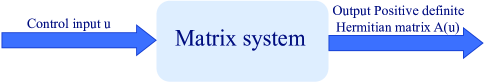
Figure 3.1: Positive definite Hermitian matrix system

The key points for designing an algorithm are then as followings:
1. To define a distance function to measure the difference between the system output and the target.
2. To computer the trajectory of input $u$ so that the output system approximates the target, as close as possible.

In order to make the matrix $A(u)$ to be as close as possible to the given target matrix $B$, we use the geodesic distance (2.8) to measure the difference between the matrices $A(u)$ and $B$. Then we are going to design a controller and obtain the $u_{*}$ such that

$$u_{*}=\arg\min_{u}J(u),$$ (3.1)

where the cost function $J(u)$ is defined by

$$J(u)=d^{2}(A(u),B).$$ (3.2)

Let the system be well defined such that

$$\mathcal{M}=\left\{A(u)\mid u=(u^{1},u^{2},\ldots.,u^{m})\in\Theta\subset\mathbb{R}^{m}\right\}$$ (3.3)

is a submanifold of manifold $P(n)$ where the control input $u$ plays the role of local coordinates.

In the following, the Riemannian gradient descent algorithm and the natural gradient descent algorithm will be used to solve this control problem, respectively. Moreover, we will analyze the suitability of two algorithms in the illustrative examples. In fact, when the target matrix $B$ lies on $\mathcal{M}$, both gradient descent algorithms are applicable. One difference is that the Riemannian gradient descent algorithm realizes the optimisation of the input trajectory while the natural gradient algorithm converges faster than the former. When the target matrix $B$ does not lie on $\mathcal{M}$, however, only the natural gradient algorithm is applicable.

3.1 The Riemannian gradient descent algorithm

Now we consider how to solve the control problem proposed above using the Riemannian gradient descent algorithm, in the case that the target matrix $B$ belongs to the output submanifold $\mathcal{M}$.

Since both the output $A(u)$ and the target matrix $B$ lie on submanifold $\mathcal{M}$, we make use of the geodesic equation to derive the trajectory and the negative gradient of the cost function $J(u)$ about $A(u)$ as the direction to give the iterative formula.

Theorem 3.1.

For the control input $u=(u^{1},u^{2},\ldots,u^{m})$ of a given positive definite Hermitian matrix system, the iterative formula is given by

$$A(u_{k+1})=A^{\frac{1}{2}}(u_{k})\exp\left\{-\eta_{k}\ln\left(A^{-\frac{1}{2}}(u_{k})BA^{-\frac{1}{2}}(u_{k})\right)\right\}A^{\frac{1}{2}}(u_{k})$$ (3.4)

where $\eta_{k}$ is the learning rate at time $k$.

Proof.

If the gradient of $J(u)$ about $A(u)$ is denoted by $\left(\nabla_{A}J\right)(u)$, then (cf. [5])

$$\left(\nabla_{A}J\right)(u_{k})=A^{\frac{1}{2}}(u_{k})\ln\left(A^{-\frac{1}{2}}(u_{k})BA^{-\frac{1}{2}}(u_{k})\right)A^{\frac{1}{2}}(u_{k}).$$ (3.5)

Recall that the Riemannian exponential map $\exp_{A}$ on manifold $P(n)$ is defined by

$$\exp_{A}\{X\}=A^{\frac{1}{2}}\exp\left\{A^{-\frac{1}{2}}XA^{-\frac{1}{2}}\right\}A^{\frac{1}{2}},$$ (3.6)

where $X$ is in the tangent space $T_{A}P(n)$. Then we obtain the iterative formula as

$$A(u_{k+1}) =\exp_{A(u_{k})}\left\{-\eta_{k}\left(\nabla_{A}J\right)(u_{k})\right\}$$ (3.7)

$$=A^{\frac{1}{2}}(u_{k})\exp\left\{-\eta_{k}A^{-\frac{1}{2}}(u_{k})\left(\nabla_{A}J\right)(u_{k})A^{-\frac{1}{2}}(u_{k})\right\}A^{\frac{1}{2}}(u_{k})$$

$$=A^{\frac{1}{2}}(u_{k})\exp\left\{-\eta_{k}\ln\left(A^{-\frac{1}{2}}(u_{k})BA^{-\frac{1}{2}}(u_{k})\right)\right\}A^{\frac{1}{2}}(u_{k}).$$

This finishes the proof. ∎

Now, we give the Riemannian gradient descent algorithm for the proposed control problem for positive definite Hermitian matrix systems.

Algorithm 3.1.

For the control input $u=(u^{1},u^{2},\ldots,u^{m})$ on a given positive definite Hermitian matrix system, the iteration algorithm is
1. Set $u_{0}=(u_{0}^{1},u_{0}^{2},\ldots,u_{0}^{m})$ as an initial input. Choose a fixed learning rate $\eta$ for simplicity and a desired tolerance $\varepsilon>0$.
2. At time $k$, calculate $A(u_{k})$ using (3.4) and $d({A(u_{k})},B)$.
3. If $d({A(u_{k})},B)<\varepsilon$ then stop. Otherwise, move to step $4$.
4. Increase $k$ by one and go back to step $2$.

Remark 3.1.

The initial output matrix $A(u_{0})$ will converge to the final output matrix $A(u_{*})$ along the geodesic connecting them, hence this algorithm realizes the trajectory optimisation of input $u$.

Remark 3.2.

If the target matrix $B$ is not on submanifold $\mathcal{M}$, it is impossible to find a geodesic on submanifold $\mathcal{M}$ such that it connects the output $A(u)$ and the target $B$. Thus, at this time, the Riemannian gradient algorithm needs be improved.

3.2 Natural gradient descent algorithm

The ordinary gradient, commonly used in learning methods on Euclidean spaces, does not give the steepest direction of a cost function on manifold, but the natural gradient does. Next, we will first introduce an important lemma about the natural gradient and then propose the natural gradient algorithm for the control problem.

Let $L(\theta)$ be a function defined in a Riemannian manifold parametrized by $\theta\in\mathbb{R}^{m}$.

Lemma 3.2 ([2]).

The natural gradient algorithm on a Riemannian manifold is given by

$$\theta_{k+1}=\theta_{k}-\eta_{k}G^{-1}{\nabla}L(\theta_{k}),$$ (3.8)

where $G^{-1}=(g^{ij})$ is the inverse of the Riemannian metric $G=(g_{ij})$, $L(\theta)$ is the cost function and

$${\nabla}L(\theta)=\left(\frac{\partial}{\partial\theta^{1}}L(\theta),\frac{\partial}{\partial\theta^{2}}L(\theta),\ldots,\frac{\partial}{\partial\theta^{m}}L(\theta)\right).$$ (3.9)

In this subsection, we will give the natural gradient descent algorithm for the considered system from the viewpoint of information geometry. This algorithm can be applied no matter whether the target matrix $B$ is on the output submanifold $\mathcal{M}$. The following lemma is useful for computing the gradient of cost function.

Lemma 3.3 ([24]).

Let $X(t)$ be a function-valued matrix of the real variable $t$ and let $A,B$ be constant matrices. We assume that, for all $t$ in its domain, $X(t)$ is an invertible matrix which does not have eigenvalues on the closed negative real line. Then

$$\frac{\operatorname{d}}{\operatorname{d}\!t}\operatorname{tr}\left(X^{\operatorname{T}}(t)X(t)\right)=2\operatorname{tr}\left(X^{\operatorname{T}}(t)\frac{\operatorname{d}}{\operatorname{d}\!t}X(t)\right),$$ (3.10)

$$\frac{\operatorname{d}}{\operatorname{d}\!t}\operatorname{tr}\left(\ln X(t)\right)=\operatorname{tr}\left(X^{-1}(t)\frac{\operatorname{d}}{\operatorname{d}\!t}X(t)\right),$$ (3.11)

$$\frac{\operatorname{d}}{\operatorname{d}\!t}\operatorname{tr}\left(AX(t)B\right)=\operatorname{tr}\left(A\frac{\operatorname{d}}{\operatorname{d}\!t}X(t)B\right).$$ (3.12)

Let $u=(u^{1},u^{2},\ldots,u^{m})$ be a parameter space on which a cost function $J(u)$ is defined, we get the following theorem.

Theorem 3.4.

The iterative process on manifold $P(n)$ is given by

$$u_{k+1}=u_{k}-\eta_{k}G^{-1}{\nabla}J(u_{k}),$$ (3.13)

where the component of gradient ${\nabla}J(u_{t})$ satisfies

$$\frac{\partial}{\partial u^{i}_{k}}J(u_{k})=2\operatorname{tr}\left(B^{-\frac{1}{2}}\ln\left(B^{-\frac{1}{2}}A(u_{k})B^{-\frac{1}{2}}\right)B^{\frac{1}{2}}A^{-1}(u_{k})\frac{\partial}{\partial u_{k}^{i}}A(u_{k})\right),~{}~{}i=1,2,\ldots,m.$$ (3.14)

Proof.

According to Lemma 3.2, we can get the iterative process as

$$u_{k+1}=u_{k}-\eta_{k}G^{-1}{\nabla}J(u_{k}),$$ (3.15)

where the Fisher metric matrix $G$ is obtained by (2.3). Let $X(u_{k})=\ln\left(A^{-\frac{1}{2}}(u_{k})BA^{-\frac{1}{2}}(u_{k})\right)$. It is easy to show that $X(t)$ is symmetric. Using Lemma 3.3, we have the fact that

$$\frac{\partial}{\partial u^{i}_{k}}J(u_{k}) =2\operatorname{tr}\left(\ln\left(B^{-\frac{1}{2}}A(u_{k})B^{-\frac{1}{2}}\right)\frac{\partial}{\partial u_{k}^{i}}\ln\left(B^{-\frac{1}{2}}A(u_{k})B^{-\frac{1}{2}}\right)\right)$$ (3.16)

$$=2\operatorname{tr}\left(B^{-\frac{1}{2}}\ln\left(B^{-\frac{1}{2}}A(u_{k})B^{-\frac{1}{2}}\right)B^{\frac{1}{2}}A^{-1}(u_{k})\frac{\partial}{\partial u_{k}^{i}}A(u_{k})\right),\quad i=1,2,\ldots,m.$$

This completes the proof of Theorem 3.4. ∎

From the above discussion, we formulate the natural gradient algorithm for the considered system as follows:

Algorithm 3.2.

For the control of the input $u=(u^{1},u^{2},\ldots,u^{m})$ on the considered Hermitian positive definite matrix system, we have the steps that
1. Set $u_{0}=(u_{0}^{1},u_{0}^{2},\ldots,u_{0}^{m})$ as an initial input. Choose a fixed learning rate $\eta$ and a desired tolerance $\varepsilon>0$.
2. At time $k$, calculate $u_{k}$ using (3.13) and ${\nabla}J(u_{k})$.
3. If $\|{\nabla}J(u_{k})\|_{F}<\varepsilon$, stop. Otherwise, move to step $4$.
4. Increase $k$ by one and go back to step $2$.

3.3 Simulations

From the following examples, we will show the efficiency of the two proposed algorithms, where the tolerance is $\varepsilon=10^{-15}$. In the first example, the target matrix $B$ lies in the submanifold $\mathcal{M}$, while it does not in the second example.

Example 3.1. We assume the target matrix $B$ is a point of the output submanifold, so both algorithms can be used. We choose a 3-dimensional input $u=(u^{1},u^{2},u^{3})$ and define the matrix system as

$$A(u)=\begin{pmatrix}u^{1}&iu^{3}\\ -iu^{3}&u^{2}\end{pmatrix},\quad u^{1}>0,u^{1}u^{2}-(u^{3})^{2}>0.$$ (3.17)

The output submanifold is then

$$\mathcal{M}_{1}=\left\{A(y;u)=\begin{pmatrix}u^{1}&iu^{3}\\ -iu^{3}&u^{2}\end{pmatrix}~{}\Big{|}~{}u^{1}>0,u^{1}u^{2}-(u^{3})^{2}>0\right\}.$$ (3.18)

We take $u_{0}^{1}=1,u_{0}^{2}=2,u_{0}^{3}=1$ as the initial input $u_{0}$ and give the target matrix $B$ by

$$B=\begin{pmatrix}55&2i\\ -2i&45\end{pmatrix},$$ (3.19)

so the coordinates of the target point $B$ is $(55,45,2)$. Using Algorithm 3.1 and Algorithm 3.2, the trajectories of the input $u$ from the initial state $A(u_{0})$ to the target matrix $B$ are obtained efficiently (see Fig. 3.3).

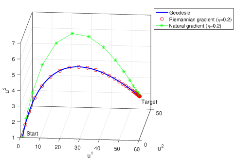
Figure 3.2: Trajectory of $u_{k}$

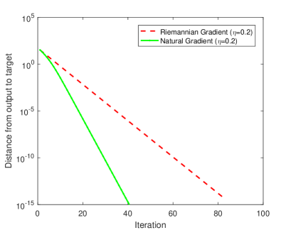
Figure 3.3: The cost function $J(u_{k})$

It is easy to see that the trajectory of the input $u$ given by the Riemannian gradient algorithm is along the geodesic connecting the initial value $u_{0}$ and the target $B$ so that the path is the shortest one. In addition, although the trajectory of the input $u$ given by the natural gradient algorithm is not optimal, the convergence is faster than the Riemannian gradient algorithm (see Fig. 3.3).

Example 3.2. Now, we consider when the target matrix $B$ does not belong to the output submanifold. In this case, only the natural gradient Algorithm 3.2 is applicable to solve the control problem. Setting the input $u$ to be a 2-dimensional vector $(u^{1},u^{2})$ and the output matrix to be that

$$A(u)=\begin{pmatrix}u^{1}&0\\ 0&u^{2}\end{pmatrix},\quad u^{1},u^{2}>0,$$ (3.20)

so output submanifold is

$$\mathcal{M}_{2}=\left\{A(u)=\begin{pmatrix}u^{1}&0\\ 0&u^{2}\end{pmatrix}~{}\Big{|}~{}u^{1},u^{2}>0\right\}.$$ (3.21)

Let us take $u_{0}^{1}=1,u_{0}^{2}=4$ as the coordinates of the initial state $A(u_{0})$ and give the target matrix $B$ by

$$B=\begin{pmatrix}50&20i\\ -20i&40\end{pmatrix}.$$ (3.22)

Then, using Algorithm 3.2 to simulate the control process, we obtain the trajectory of the input $u$ from the initial state $A(u_{0})$ to the approximate matrix $A(u_{*})$ of the target matrix $B$ efficiently. The coordinate of $A(u_{*})$ is $u_{*}=(44.721,35.777)$ which can be taken as the geodesic projection of the target $B$ onto submanifold $\mathcal{M}_{2}$ (see Fig. 3.5). Furthermore, when we set the learning rate $\eta=0.1,0.2,0.5$ respectively, the efficiency and the convergence of Algorithm 3.2 are shown by Fig. 3.5.

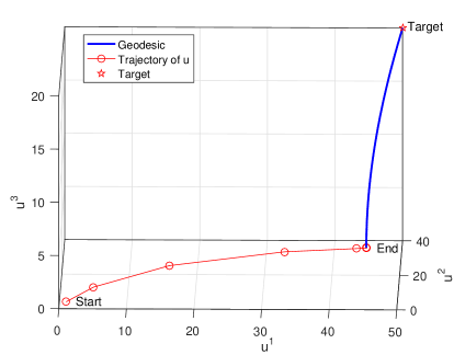
Figure 3.4: Geodesic projection from target onto $\mathcal{M}_{2}$

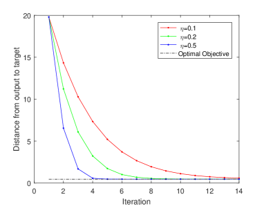
Figure 3.5: Convergence of the natural gradient

4 Karcher mean of Toeplitz positive definite Hermitian matrices

Mean of matrices plays an important role in many fields, such as numerical analysis, probability and statistics, engineering, biological and social sciences (cf. [1, 6, 18, 22]). Many algorithms have been developed to computer such means, see e.g. ([7, 11, 21]). For electromagnetic or acoustic sensors, and more especially for radar, lidar or echography, it is necessary to consider the spatial complex data for the array processing or the time complex data for the Doppler processing: $Z_{n}=[z_{1},z_{2},\ldots,z_{n}]^{\operatorname{T}}$(cf. [5]). The covariance matrices of these complex data $R_{n}=E[Z_{n}Z_{n}^{\operatorname{H}}]$ are the Toeplitz positive definite Hermitian matrices

$$R_{n}=\begin{pmatrix}r_{0}&\overline{r}_{1}&\cdots&\overline{r}_{n-1}\\ r_{1}&r_{0}&\ddots&\vdots\\ \vdots&\ddots&\ddots&\overline{r}_{1}\\ r_{n-1}&\cdots&r_{1}&\overline{r}_{0}\end{pmatrix},$$ (4.1)

where $r_{k}=E[z_{n}\overline{z}_{n-k}]$ and $Z^{\operatorname{H}}R_{n}Z>0,$ for $\forall Z\in\mathbb{C}^{n}$.

In this section, we consider the complex circular multivariate Gaussian distribution of zero mean with probability density function

$$p(Z_{n}|R_{n})=\frac{1}{\pi^{n}\det(R_{n})}\exp\left\{-Z_{n}^{\operatorname{H}}R_{n}^{-1}Z_{n}\right\}.$$ (4.2)

Let us denote the set of all $n\times n$ Toeplitz positive definite Hermitian matrices by $Sym(n,\mathbb{C})$ which is obviously an $(n^{2}-n+1)$-dimensional submanifold of manifold $P(n)$. In the Riemannian sense, the mean $\overline{R}$ of $N$ given positive definite Hermitian matrices $R^{1},R^{2},\ldots,R^{N}$ is defined as [10]

$$\overline{R}=\arg\min_{R\in Sym(n,\mathbb{C})}\frac{1}{N}\sum_{i=1}^{N}d^{2}(R^{i},R),$$ (4.3)

which is called the Karcher mean. For $N$ distributions $p(\cdot|R^{i}),i=1,2,\ldots,N$, we denote their covariance matrices by $R^{k}$ and define the cost function by

$$L(R)=\frac{1}{N}\sum_{i=1}^{N}d^{2}(R^{i},R).$$ (4.4)

Note that the local curvature of complex circular multivariate Gaussian distribution of zero mean is a non-positive constant, so the Karcher mean is unique [14].

In [4], it was shown that the Jacobi field for the Karcher mean vanishes. In order to estimate the Doppler ambiance, Barbaresco [5] computed the Jacobi field and proposed the Riemannian gradient algorithm to compute the Karcher Mean by

$$R_{k+1}=R_{k}^{\frac{1}{2}}\exp\left\{-\eta\sum_{i=1}^{N}\ln\left(R_{k}^{-\frac{1}{2}}R^{i}R_{k}^{-\frac{1}{2}}\right)\right\}R_{k}^{\frac{1}{2}}$$ (4.5)

with $\eta$ the learning rate.

In the following, we will propose the natural gradient algorithm to compute the Karcher mean of $N$ Toeplitz positive definite Hermitian matrices $R^{i}(i=1,2,\ldots,N)$ followed with simulations.

4.1 Natural gradient descent algorithm

Let $\theta=(\theta^{1},\theta^{2},\ldots,\theta^{m})$ be a parameter space on which a function $L(\theta)$ is defined. Analogously to the proof of Theorem 3.4, we have the following theorem:

Theorem 4.1.

The iterative process on manifold $Sym(n,\mathbb{C})$ is given by

$$\theta_{k+1}=\theta_{k}-\eta G^{-1}{\nabla}|_{\theta=\theta_{k}}L(\theta),$$ (4.6)

where

$${\nabla}L(\theta)=\left(\frac{\partial}{\partial\theta^{1}}L(\theta),\frac{\partial}{\partial\theta^{2}}L(\theta),\ldots,\frac{\partial}{\partial\theta^{m}}L(\theta)\right),$$ (4.7)

and the component of gradient ${\nabla}L(\theta)$ satisfies

$$\frac{\partial}{\partial\theta^{j}}L(\theta)=\frac{2}{N}\operatorname{tr}\left(\sum_{i=1}^{N}R_{i}^{-\frac{1}{2}}\ln\left(R_{i}^{-\frac{1}{2}}RR_{i}^{-\frac{1}{2}}\right)R_{i}^{\frac{1}{2}}R^{-1}\frac{\partial}{\partial\theta^{j}}R\right),\quad j=1,2,\ldots,m.$$ (4.8)

Now we are ready to formulate the natural gradient algorithm.

Algorithm 4.1.

The natural gradient algorithm to computer the Karcher mean of $N$ matrices of the manifold $Sym(n,\mathbb{C})$ is as follows:
1. Take the arithmetic mean $\frac{1}{N}\sum_{i=1}^{N}R^{i}$ as the initial point $\theta_{0}$. Choose a learning rate $\eta$ and a desired tolerance $\varepsilon>0$.
2. At time $k$, calculate $\theta_{k}$ using (4.6) and ${\nabla}L(\theta_{k})$.
3. If $\|{\nabla}L(\theta_{k})\|<\varepsilon$, stop. Otherwise, move to step $4$.
4. Increase $k$ by one and go back to step $2$.

4.2 Simulations

In this subsection, we use the two gradient descent algorithms mentioned above to compute Karcher mean of $N$ given Toeplitz positive definite Hermitian matrices, where the tolerance is again $\varepsilon=10^{-15}$. From the following examples, it is shown that the natural gradient algorithm is more efficient than the algorithm (4.5).

For simplicity, we choose a 2-dimensional spatial complex data for the array processing or the time complex data for the Doppler processing: $Z_{2}=[z_{1},z_{2}]^{\operatorname{T}}$. Then, the covariance matrices of these complex data can be written as

$$\begin{pmatrix}\theta_{1}&\theta_{2}+\operatorname{i}\theta_{3}\\ \theta_{2}-\operatorname{i}\theta_{3}&\theta_{1}\end{pmatrix}.$$ (4.9)

Example 4.1. We computer the Karcher mean of $R^{1},R^{2}$ on manifold $Sym(2,\mathbb{C})$ as a first example, where

$$R^{1}=\begin{pmatrix}5&1+2\operatorname{i}\\ 1-2\operatorname{i}&5\end{pmatrix},\quad R^{2}=\begin{pmatrix}4&1-\operatorname{i}\\ 1+\operatorname{i}&4\end{pmatrix}.$$ (4.10)

In fact, it is easy to know their Karcher mean $R^{1}\circ R^{2}$ corresponds to (2.7). To show the algorithm’s efficiency, the natural gradient algorithm and the algorithm (4.5) are used respectively. Choose the arithmetic mean $\frac{1}{2}\sum_{i=1}^{2}R^{i}$ as the initial point $\theta_{0}$. On manifold $Sym(2,\mathbb{C})$, the adjustment of the coordinate vector $\theta$ is given by (4.5) and (4.6). From (2.6), the geodesic between $R^{1}$ and $R^{2}$ is computed (see Fig. 4.1). We denote the Karcher mean by a red pentacle. It is shown that both algorithms converge to the red pentacle. It is also shown that the natural gradient algorithm (4.6) converges faster than the algorithm (4.5) (see Fig. 4.2).

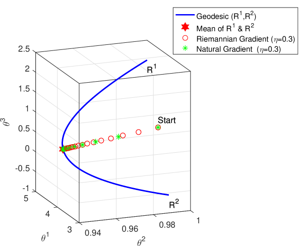
Figure 4.1: Iterative process

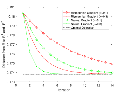
Figure 4.2: Descent process of the cost function

Example 4.2. Here, we consider three $2\times 2$ Toeplitz positive definite Hermitian matrices

$$R^{1}=\begin{pmatrix}3&1.5+2\operatorname{i}\\ 1.5-2\operatorname{i}&3\end{pmatrix},\quad R^{2}=\begin{pmatrix}2&1-\operatorname{i}\\ 1+\operatorname{i}&2\end{pmatrix},\quad R^{3}=\begin{pmatrix}4&1+2\operatorname{i}\\ 1-2\operatorname{i}&4\end{pmatrix}.$$ (4.11)

Using (2.6), we can get the geodesics between each two of the three points $R^{1},R^{2}$ and $R^{3}$ on $Sym(2,\mathbb{C})$, which form a geodesic triangle (see Fig. 4.4). The midpoint of each geodesic is obtained using (2.7). Thus, each median connects a vertex with the midpoint of its opposing side. In Euclidean spaces, these centerlines always meet in a single point which is the Karcher mean. However, in curved spaces, as Fig. 4.4 shows, this is no longer true. In fact, when we change the look angle to Fig. 4.4, it is shown that three midlines are very likely non-coplanar (see Fig. 4.4).

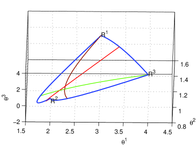
Figure 4.3: Geodesic triangle (position 1)

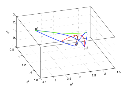
Figure 4.4: Geodesic triangle (position 2)

Now we compute the Karcher mean $p(\cdot|\overline{R})$ of 3 distributions $p(\cdot|R^{i}),i=1,2,3$ using these two algorithms. Similarly to Example 4.1, first we still take the arithmetic mean $\frac{1}{3}\sum_{i=1}^{3}R^{i}$ as the initial point $\theta_{0}$ . On manifold $Sym(2,\mathbb{C})$, the adjustment of the coordinate vector $\theta$ is given by (4.5) and (4.6). Finally, both algorithms converge to the Karcher mean (see Fig. 4.5)

$$\overline{R}=\arg\min_{R\in Sym(2,\mathbb{C})}\frac{1}{3}\sum_{i=1}^{3}d^{2}(R^{i},R)=\begin{pmatrix}2.295&0.980+0.617\operatorname{i}\\ 0.980-0.617\operatorname{i}&2.295\end{pmatrix}.$$ (4.12)

Again the natural gradient algorithm is faster than the algorithm (4.5) (see Fig. 4.6).

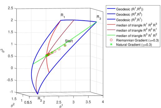
Figure 4.5: Convergence from initial point to the Karcher mean

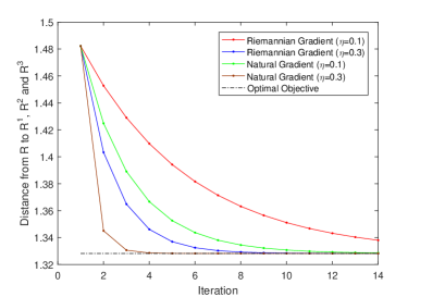
Figure 4.6: Descent process of the cost function

5 Conclusions

In this paper, we applied the Riemannian gradient algorithm and the natural gradient algorithm to the control of positive Hermitian matrix systems as well as the computation of Karcher mean of Toeplitz positive definite Hermitian matrices. Their behaviors were also compared.

For the control system, when the target matrix belongs to the output submanifold, the Riemannian gradient descent algorithm and the natural gradient algorithm are both applicable. It was shown that the former realizes the optimisation of input trajectory while the latter has preferable convergence. We also proposed the natural gradient algorithm to compute the Karcher mean of matrices in the submanifold $Sym(n,\mathbb{C})$, taking the sum of geodesic distances as the cost function. The simulations showed that convergence rate of the natural gradient algorithm is faster than the Riemannian gradient algorithm, which has been widely used to solve such optimisation problems during the last decade.

References

- [1] R. Adamczak, A.E. Litvak, A. Pajor and N. Tomczak-Jaegermann, Quantitative estimates of the convergence of the empirical covariance matrix in Log-concave ensemble, J. Amer. Math. Soc. 23 (2010), 535–561.
- [2] S. Amari, Natural gradient works efficiently in learning, Neural Comput. 10 (1998), 251–276.
- [3] S. Amari and S.C. Douglas, Why natural gradient? ICASSP, pp. 1213–1216, 1998.
- [4] M. Arnaudon and X.M. Li, Barycentres of measures transported by stochastic flows, Ann. Probab. 33 (2005), 1509–1543.
- [5] F. Barbaresco, Interactions between symmetric cones and information geometries: Bruhat–Tits and Siegel spaces models for high resolution autoregressive Doppler imagery, ETCV’08, Springer Lecture Notes in Computer Science, pp. 124–163, 2009.
- [6] R. Bhatia, T. Jain and Y. Lim, Inequalities for the Wasserstein mean of positive definite matrices, Linear Algebra Appl., 2019, in press.
- [7] Z. Chebbi and M. Moakher, Means of Hermitian positive-definite matrices based on the log-determinant -divergence function, Linear Algebra Appl. 436 (2012), 1872–1889.
- [8] X. Duan, H. Sun and X. Zhao, Riemannian Gradient Algorithm for the Numerical Solution of Linear Matrix Equations, J. Appl. Math., 2014(2) (2014), Article ID 507175, 7pp.
- [9] H. Gozde, M.C. Taplamacioglu and İ. Kocaarslan, Comparative performance analysis of Artificial Bee Colony algorithm in automatic generation control for interconnected reheat thermal power system, Int. J. Elec. Power 42 (2012), 167–178.
- [10] K. Grove, H. Karcher and E.A. Ruh, Jacobi fields and Finsler metrics on compact Lie groups with an application to differentiable pinching problem, Math. Ann. 211 (1974), 7–22.
- [11] A. Guven, Approximation of Continuous Functions by Matrix Means of Hexagonal Fourier Series, Results Math. 73:18 (2018), 25pp.
- [12] C.S. Hughes, S.D. Patek, M. Breton and B.P. Kovatchev, Anticipating the next meal using meal behavioral profiles: a hybrid model-based stochastic predictive control algorithm for T1DM, Comput. Methods Programs Biomed. 102 (2011), 138–148.
- [13] J. Jost, Riemannian Geometry and Geometric Analysis, 3rd edn., Springer, Berlin, 2002.
- [14] H. Karcher, Riemannian center of mass and mollifier smoothing, Commun. Pure Appl. Math. 30 (1977), 509–541.
- [15] B.G. Kim and J.W. Lee, Stochastic utility-based flow control algorithm for services with time-varying rate requirements, Comput. Netw. 56 (2012), 1329–1342.
- [16] C. Lenglet, M. Rousson, R. Deriche and O. Faugeras, Statistics on the Manifold of Multivariate Normal Distributions: Theory and Application to Diffusion Tensor MRI Processing, J. Math. Imaging Vis. 25 (2006), 423–444.
- [17] C. Li, E. Zhang, J. Lin and H. Sun, Optimal control on special Euclidean group via natural gradient algorithm, Sci. China Inf. Sci. 59:112203 (2016), 10pp.
- [18] J.K. Liu, X. Wang, T. Wang and L.H. Qu, Application of information geometry to target detection for pulsed-Doppler radar, Journal of National University of Defense Technology 33 (2011), 77–80.
- [19] M. Moakher, A differential geometric approach to the geometric mean of symmetric positive-definite matrices, SIAM J. Matrix Anal. Appl. 26 (2005), 735–747.
- [20] M. Moakher, On the averaging of symmetric positive-pefinite tensors, J. Elast. 82 (2006), 273–296.
- [21] E. Nobari and B.A. Kakavandi, A geometric mean for Toeplitz and Toeplitz-block block-Toeplitz matrices, Linear Algebra Appl. 548 (2018), 189–202.
- [22] R. Takahashi, N. Yoshida, M. Takada, et al., Simulations of baryon acoustic oscillations II: Covariance matrix of the matter power spectrum, Astrophys. J. 700 (2009), 479–490.
- [23] Y. Tang and J. Li, Normalized natural gradient in independent component analysis, Signal Processing 90 (2010), 2773–2777.
- [24] X. Zhang, Matrix Analysis and Applications, Tsinghua University Press, Beijing, 2004.
- [25] Z. Zhang, H. Sun and L. Peng and L. Jiu, A Natural Gradient Algorithm for Stochastic Distribution Systems, Entropy 16 (2014), 4338–4352.
- [26] J. Zhao and X. Yu, Adaptive natural gradient learning algorithms for Mackey–Glass chaotic time prediction, Neurocomputing 157 (2015), 41–45.