Transfer Learning for Performance Modeling of Deep Neural Network Systems

Abstract

Modern deep neural network (DNN) systems are highly configurable with large a number of options that significantly affect their non-functional behavior, for example inference time and energy consumption. Performance models allow to understand and predict the effects of such configuration options on system behavior, but are costly to build because of large configuration spaces. Performance models from one environment cannot be transferred directly to another; usually models are rebuilt from scratch for different environments, for example different hardware. Recently, transfer learning methods have been applied to reuse knowledge from performance models trained in one environment in another. In this paper, we perform an empirical study to understand the effectiveness of different transfer learning strategies for building performance models of DNN systems. Our results show that transferring information on the most influential configuration options and their interactions is an effective way of reducing the cost to build performance models in new environments.

1 Introduction

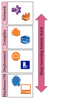
Figure 1: DNN System Stack

Deep neural networks (DNNs) are becoming increasingly complex, with an increased number of parameters to tune, and increased energy consumption for the deployed system [19]. Current state-of-the-art methods for tuning DNNs do not consider how a DNN is deployed in a system stack [1, 19, 2], and do therefore not consider energy consumption. Figure 1 shows a $4$-level deployment environment of a DNN system where options and option interactions from each level contribute to energy consumption [10, 14, 11].

Performance models have been extensively used for understanding the behavior of configurable systems [5, 6, 16, 17, 22, 24]. However, constructing such models requires extensive experimentation because of large parameter spaces, complex interactions, and unknown constraints [23]. Such models are usually designed for fixed environments, i.e., fixed hardware and fixed workloads, and cannot be used directly when the environment changes. Repeating the process of building a performance model every time an environment change occurs is costly and slow. Several transfer learning approaches have been proposed to reuse information from performance models in a new environment for different configurable systems [9, 10, 8, 4]; however, to the best of our knowledge, no approach focuses specifically on DNNs in different environments. We consider the following research question:

How can we efficiently and effectively transfer information from a performance model of a DNN trained for one environment to another environment?

We perform an empirical study comparing different transfer learning strategies for performance models of DNNs for different environmental changes, e.g., different hardware and different workloads. We consider guided sampling (GS)[9], direct model transfer (DM) [21], linear model shift (LMS), and non-linear model shift (NMLS)[10]. We model the non-functional properties inference time and energy consumption in this paper and consider configuration options that affect these properties as the parameters we tune, i.e. hardware-level configuration options. Our results indicate that GS transfer learning outperforms next best learning method, NMLS, by $19.76\%$ and $8.33\%$ using regression trees (RT) and by $23.47\%$ and $12.70\%$ using neural networks (NN) for inference time and energy consumption, respectively. This enabled us to build performance models in new environments using only $2.44\%$ of the configuration space to predict best configurations in our systems with comparable accuracy to the performance models built for the original environment.The difference between the lowest and highest energy consumption can be up to a factor of 20.

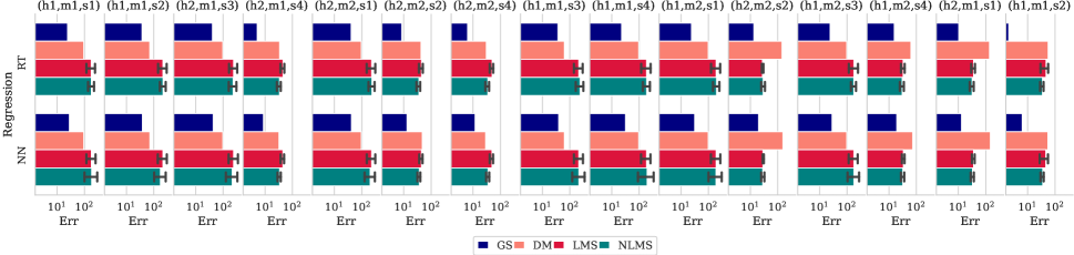
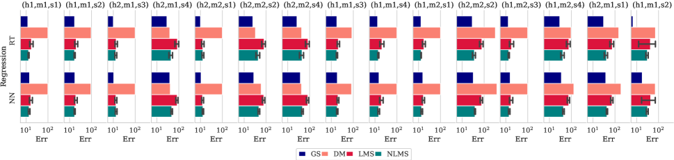
Figure 2: Comparison of prediction error of different transfer learning techniques (GS, DM, LMS, and NLMS) for performance models of DNN systems (Regression Tree and Neural Net) for inference time (top) and energy consumption (bottom). We consider 15 different target environments and show error bars for values aggregated over 10 predictions on a log scale.

2 Methodology

We consider a pre-trained image recognition DNN system in 16 different environments: 2 different hardware platforms (Nvidia Jetson TX1, $h_{1}$, and Jetson TX2, $h_{2}$), 2 pre-trained models (Xception[3], $m_{1}$, and InceptionV3[20], $m_{2}$) and 4 different image sizes ($200\times{}200$, $400\times{}400$, $600\times{}600$, and $800\times{}800$, $s_{1}$ through $s_{4}$). In each environment, we evaluate the performance on the same 10 randomly selected images from the ILSVRC2017[15] image recognition dataset.

The configuration space we consider is composed of the following hardware configuration options: (1) CPU status, (2) CPU frequency, (3) GPU frequency, and (4) memory controller frequency. We evaluate a total of 46,080 configurations on the TX1 platform and 11,616 configurations on the TX2 platform, for a total experimental effort of $\approx$ 43.6 days of computational time across all 16 environments. We chose the TX1 and TX2 platforms due to their limited energy budget to better understand DNN system behavior with changing configuration options.

We construct performance models of the effect of configuration options on DNN system performance using these experimental data with RTs and NNs, which are frequently used in the literature to induce performance models [5, 21, 16, 12, 13]. We measure the performance of these models in terms of mean absolute percentage error, Err[18].

We implement GS using a step-wise regression technique with forward selection (FS) and backward elimination (BE). Each step of FS adds an interaction term to the regression model that increases the coefficient of determination, while BE removes an interaction term if its significance is below a threshold. We study the interaction terms of the final regression model; in particular, we exclude terms with coefficients that are less than $10^{-12}$. These terms guide the sampling towards important configuration options and avoid wasting resources on evaluations that effect no change when building performance models in new environments. The DM transfer learning approach reuses a performance model built for one environment directly in a different environment. The LMS and NMLS transfer learning techniques learn a linear regression model and a non-linear random forest regression model, respectively, to translate the predictions from a performance model trained for one environment into predictions for a different environment. These transfer models are based on a small number of randomly-sampled configurations that are evaluated in both environments.

In our experiments, we select the TX2 platform with the InceptionV3 DNN and $600\times{}600$ images as the source environment to train the performance models for. We transfer these performance models to each of the remaining 15 target environments. The source code and data are available in an online appendix [7].

3 Results and Discussion

We present the results in Figure 2. They demonstrate that GS outperforms DM, LMS, and NMLS in each environment for both inference time and energy consumption. Average Err of the performance models induced using GS are $28.09\%$ and $22.93\%$ lower than DM, $25.64\%$ and $21.59\%$ lower than LMS, and $23.47\%$ and $19.76\%$ lower than NLMS for inference time using NN and RT, respectively. Similarly, they are $42.85\%$ and $39.41\%$ lower than DM, $20.52\%$ and $13.19\%$ lower than LMS, and $12.70\%$ and $8.33\%$ lower than NLMS for energy consumption for NN and RT, respectively. All of GS, LMS, and NLMS incurred the same cost (evaluation of $2.44\%$ of the entire configuration space, $\approx$ 2.48 hours), while the cost for DM was zero as the performance model from the source environment is reused without modification in the target environment. For the DM and GS transfer learning techniques, an increase in computational effort of just 2.48 hours ($\approx$ 0.15% of the effort to train the original performance model) leads to an decrease of ${\sf Err}$ of $28.09\%$ and $22.93\%$ for inference time and $42.85\%$ and $39.41\%$ for energy consumption using NN and RT, consecutively.

If the environment change between source and target includes a hardware change, DM is more effective than LMS and NLMS for inference time modeling; however, for energy consumption, NLMS performs better than DM and LMS.

Guided sampling can help practitioners to quickly develop reliable performance models for new environments based on information they have obtained in the past to tune and optimize a system. Such performance models can guide practitioners to avoid invalid configurations and are useful for design space exploration to quickly find optimal configurations in new environments using influential configurations which typically practitioners miss. These models are also useful to learn the performance landscape of a system for performance debugging, and obtain a better understanding of how the configuration options affect performance in general. In future work, we will consider extending the configuration space with options from all $4$ levels of the DNN system stack.

4 Acknowledgements

This work has been supported by AFRL and DARPA (FA8750-16-2-0042). Lars Kotthoff is supported by NSF grant #1813537.

References

- [1] Ermao Cai, Da-Cheng Juan, Dimitrios Stamoulis, and Diana Marculescu. Neuralpower: Predict and deploy energy-efficient convolutional neural networks. arXiv:1710.05420, 2017.
- [2] Yu-Hsin Chen, Joel Emer, and Vivienne Sze. Eyeriss: A spatial architecture for energy-efficient dataflow for convolutional neural networks. In ACM SIGARCH Computer Architecture News, volume 44, pages 367–379. IEEE Press, 2016.
- [3] François Chollet. Xception: Deep learning with depthwise separable convolutions. arXiv preprint, pages 1610–02357, 2017.
- [4] Daniel Geschwender, Frank Hutter, Lars Kotthoff, Yuri Malitsky, Holger H. Hoos, and Kevin Leyton-Brown. Algorithm Configuration in the Cloud: A Feasibility Study. In LION 8, pages 41–44, February 2014.
- [5] Jianmei Guo, Krzysztof Czarnecki, Sven Apel, Norbert Siegmund, and Andrzej Wasowski. Variability-aware performance prediction: A statistical learning approach. In Proc. Int’l Conf. Automated Software Engineering (ASE), pages 301–311. IEEE, 2013.
- [6] Henry Hoffmann, Stelios Sidiroglou, Michael Carbin, Sasa Misailovic, Anant Agarwal, and Martin Rinard. Dynamic knobs for responsive power-aware computing. In In Proc. of Int’l Conference on Architectural Support for Programming Languages and Operating Systems (ASPLOS), 2011.
- [7] Md Shahriar Iqbal, editor. Opml-DNNPerfModeling. 2019. https://github.com/iqbal128855/OpML19-DNNPerfModeling.
- [8] Pooyan Jamshidi, Norbert Siegmund, Miguel Velez, Christian Kästner, Akshay Patel, and Yuvraj Agarwal. Transfer learning for performance modeling of configurable systems: An exploratory analysis. In Proceedings of the 32nd IEEE/ACM International Conference on Automated Software Engineering (ASE), pages 497–508. IEEE Press, 2017.
- [9] Pooyan Jamshidi, Miguel Velez, Christian Kästner, and Norbert Siegmund. Learning to sample: exploiting similarities across environments to learn performance models for configurable systems. In Proceedings of the 2018 26th ACM Joint Meeting on European Software Engineering Conference and Symposium on the Foundations of Software Engineering (ESEC/FSE), pages 71–82. ACM, 2018.
- [10] Pooyan Jamshidi, Miguel Velez, Christian Kästner, Norbert Siegmund, and Prasad Kawthekar. Transfer learning for improving model predictions in highly configurable software. In Proceedings of the 12th International Symposium on Software Engineering for Adaptive and Self-Managing Systems (SEAMS), pages 31–41. IEEE Press, 2017.
- [11] Irene Manotas, Lori Pollock, and James Clause. Seeds: a software engineer’s energy-optimization decision support framework. In Proceedings of the 36th International Conference on Software Engineering (ICSE), pages 503–514. ACM, 2014.
- [12] Vivek Nair, Tim Menzies, Norbert Siegmund, and Sven Apel. Faster discovery of faster system configurations with spectral learning. Automated Software Engineering (ASE), pages 1–31, 2017.
- [13] Vivek Nair, Tim Menzies, Norbert Siegmund, and Sven Apel. Using bad learners to find good configurations. In Proc. Int’l Symp. Foundations of Software Engineering (FSE), ESEC/FSE 2017, pages 257–267, New York, NY, USA, 2017. ACM.
- [14] Hang Qi, Evan R Sparks, and Ameet Talwalkar. Paleo: A performance model for deep neural networks. 2016.
- [15] Olga Russakovsky, Jia Deng, Hao Su, Jonathan Krause, Sanjeev Satheesh, Sean Ma, Zhiheng Huang, Andrej Karpathy, Aditya Khosla, Michael Bernstein, Alexander C. Berg, and Li Fei-Fei. ImageNet Large Scale Visual Recognition Challenge. International Journal of Computer Vision (IJCV), 115(3):211–252, 2015.
- [16] Atri Sarkar, Jianmei Guo, Norbert Siegmund, Sven Apel, and Krzysztof Czarnecki. Cost-efficient sampling for performance prediction of configurable systems. In Proc. Int’l Conf. Automated Software Engineering (ASE), pages 342–352. IEEE, November 2015.
- [17] Norbert Siegmund, Alexander Grebhahn, Sven Apel, and Christian Kästner. Performance-influence models for highly configurable systems. In Proc. Europ. Software Engineering Conf. Foundations of Software Engineering (ESEC/FSE), pages 284–294. ACM, August 2015.
- [18] P. M. Swamidass. Mape (mean absolute percentage error)mean absolute percentage error (mape). In Encyclopedia of Production and Manufacturing Management, pages 462–462, Boston, MA, 2000. Springer US.
- [19] Vivienne Sze, Yu-Hsin Chen, Tien-Ju Yang, and Joel S Emer. Efficient processing of deep neural networks: A tutorial and survey. Proceedings of the IEEE, 105(12):2295–2329, 2017.
- [20] Christian Szegedy, Vincent Vanhoucke, Sergey Ioffe, Jon Shlens, and Zbigniew Wojna. Rethinking the inception architecture for computer vision. In Proceedings of the IEEE conference on computer vision and pattern recognition (CVPR), pages 2818–2826, 2016.
- [21] Pavel Valov, Jean-Christophe Petkovich, Jianmei Guo, Sebastian Fischmeister, and Krzysztof Czarnecki. Transferring performance prediction models across different hardware platforms. In Proc. Int’l Conf. on Performance Engineering (ICPE), pages 39–50. ACM, 2017.
- [22] Fan Wu, Westley Weimer, Mark Harman, Yue Jia, and Jens Krinke. Deep parameter optimisation. In Proc. of the Annual Conference on Genetic and Evolutionary Computation (GECCO), pages 1375–1382. ACM, 2015.
- [23] Tianyin Xu, Long Jin, Xuepeng Fan, Yuanyuan Zhou, Shankar Pasupathy, and Rukma Talwadker. Hey, you have given me too many knobs!: Understanding and dealing with over-designed configuration in system software. In Proc. Int’l Symp. Foundations of Software Engineering (FSE), pages 307–319, New York, NY, USA, August 2015. ACM.
- [24] Nezih Yigitbasi, Theodore L Willke, Guangdeng Liao, and Dick Epema. Towards machine learning-based auto-tuning of mapreduce. In Proc. Int’l Symp. on Modeling, Analysis and Simulation of Computer and Telecommunication Systems (MASCOTS), pages 11–20. IEEE, 2013.