A Critical Evaluation of Recent Claims Concerning Solar Rotation

Abstract

Fossat et al. (2017) recently reported detecting rotational splitting of g modes indirectly via the interaction with p modes observed directly by the GOLF instrument on SOHO. They concluded that the core of the Sun is rotating $3.8\pm 0.1$ times faster than the surrounding radiative envelope. This is startling, partly because such rapid rotation almost contradicts direct inferences from the p-mode rotational splitting inferred from the same data. Moreover, the inferred amplitudes of the g modes appear to exceed the upper bound reported by Appourchaux et al. (2010). It is also suspect because the theory of the procedure implies that the principal modes claimed to have been measured should be undetectable. We point out that there are other interpretations: one leads to a core rotation about twice faster than the surrounding envelope; another, to a core rotating more slowly than the envelope. Here we also report on an independent assessment of the Fossat et al. analysis by applying their procedure to different representations of the GOLF data, expanding on Schunker et al. (2018). We also analyze seismic data obtained from LOI and MDI (both also on SOHO), from HMI (on SDO) and from the ground-based BiSON and GONG, and found the evidence reported by Fossat et al. not to be robust. We also illustrate that merely fitting model spectra to observations, which Fossat et al. do to support their g-mode detections and as Fossat & Schmider (2018) do for extracting additional g-mode splittings, is not necessarily reliable. We are therefore led to doubt the claim.

1 Introduction

The density and pressure perturbations, and the associated velocity field, produced by g modes modify the propagation of acoustic waves and so influence the p-mode frequencies. As Kennedy et al. (1993) have pointed out, that, in principle, offers a potential probe of the dynamics of solar g modes of even degree, and may be the only way in which accurate constraints on the structure and kinematics of the innermost regions of the Sun can be accessed.

The influence of high-order g modes of low degree can most easily be estimated by noting that the g-mode frequencies are much lower than those of the p modes, and that therefore to a first approximation the effectively instantaneous p-mode frequencies $\omega$ can be estimated by ignoring the explicit g-mode time dependence. The time dependence of the global angular velocity can be ignored too. In that extreme case, g modes modify the frequency of any particular p mode independently of the others, and then the variational integral relation of Lynden-Bell & Ostriker (1967) can be brought to bear to characterize the p-mode frequencies:

$${\cal I}\omega^{2}-2{\cal R}\omega-{\cal K}=0\,,$$ (1)

where ${\cal I}({\boldsymbol{\xi}^{*},\boldsymbol{\xi}})$, ${\cal R}(\boldsymbol{\xi}^{*},\boldsymbol{\xi})$ and ${\cal K}(\boldsymbol{\xi}^{*},\boldsymbol{\xi})$ are integrals depending on the instantaneous underlying state of the star, including the (small) contribution from the g modes but not from the p modes. They depend explicitly on the (complex) adiabatic p-mode displacement eigenfunction $\boldsymbol{\xi}($r$){\rm e}^{{\rm-i}\omega t}$, where r is a position vector in an inertial frame centred on the star, and $t$ is time. Also ${\rm i}=\sqrt{(}-1)$. The integrals are over the volume $\cal V$ of the star; they are given approximately by

$${\cal I}({\boldsymbol{\xi}^{*},\boldsymbol{\xi}})=\int_{\cal V}\boldsymbol{\xi}^{*}.\,\boldsymbol{\xi}\rho{\rm d}V\,,$$ (2)

$${\cal R}({\boldsymbol{\xi}^{*},\boldsymbol{\xi}})={\rm i}\int_{\cal V}\boldsymbol{\xi}^{*}.(\textbf{{v}}.\nabla\boldsymbol{\xi})\rho{\rm d}V$$ (3)

and

$${\cal K}({\boldsymbol{\xi}^{*},\boldsymbol{\xi}})=\int_{\cal V}[\rho c^{2}{\rm div}{\boldsymbol{\xi}^{*}}{\rm div}\boldsymbol{\xi}+(\boldsymbol{\xi}^{*}{\rm div}{\boldsymbol{\xi}}+\boldsymbol{\xi}{\rm div}{\boldsymbol{\xi}^{*}}).\nabla p+\rho^{-1}\boldsymbol{\xi}^{*}.\nabla\rho\;\boldsymbol{\xi}.\nabla p]\,{\rm d}V$$ (4)

(cf. Gough, 1993), in which $p$ is pressure, $\rho$ is density and $c$ is the adiabatic sound speed. The asterisk denotes complex conjugate. The vector v is the background fluid velocity, which accommodates both the angular velocity $\Omega(r,\theta)$, with respect to spherical polar coordinates $(r,\theta,\phi)$, and the (real) velocity $\boldsymbol{u}$ associated with the g modes. For simplicity, we ignore steady meridional circulation. We are therefore presuming the angular velocity to be about the unique axis about which the co-ordinates $(r,\theta,\phi)$ are defined. Because both the p modes and the g modes are of high order, the Cowling approximation (in which the Eulerian perturbation to the gravitational potential is ignored) has been adopted, and for added simplicity a small surface boundary term has been neglected. It would be straightforward to include them. In addition, terms quadratic in $\Omega(r,\theta)$ and in the g-mode perturbation are also neglected. As Lynden-Bell & Ostriker (1967) demonstrated, the integral $\cal R$ is skew symmetric, and $\cal I$ and $\cal K$ are symmetric in $\xi^{*}$ and $\xi$; equation (1) constitutes a variational principle for the p modes, and therefore it is sufficient to employ the displacement eigenfunction $\boldsymbol{\xi}$ of what we call the basic state, namely a spherically symmetric model of the Sun (in which $\nabla p$ and $\nabla\rho$ are both radially directed, and ${\cal K}$ is therefore obviously symmetric), unperturbed by rotation and the modes of oscillation.

The eigenfunctions of the basic state are of the form

$$\boldsymbol{\xi}_{n,l,m}({\boldsymbol{r}})=\left(\xi_{n,l}(r)P^{m}_{l},\frac{\eta_{n,l}(r)}{L}\frac{{\rm d}P^{m}_{l}}{{\rm d}\theta},\frac{{\rm i}m\eta_{n,l}(r)}{L\,{\rm sin}\theta}P^{m}_{l}\right){\rm e}^{{\rm i}m\phi}\,,$$ (5)

$$\psi_{n,l,m}({\boldsymbol{r}})=\psi_{n,l}(r)P^{m}_{l}{\rm e}^{{\rm i}m\phi}\,,$$ (6)

where $\psi$ is a scalar component of the oscillation eigenfunction such as the pressure or density perturbation; $P^{m}_{l}({\rm cos}\theta)$ is the associated Legendre function of the first kind, of degree $l$ and order $m$; and $L=\sqrt{l(l+1)}$. We adopt the normalization $P^{-m}_{l}({\rm cos}\theta)=P^{m}_{l}({\rm cos}\theta)$. The modes can be characterized by their order $n$, degree $l$ and azimuthal order $m$. We note that the modes are degenerate in $m$: any group of modes of like $n$ and $l$ and varying $m$, having a common frequency, is called a multiplet; the individual modes are singlets. Degeneracy is lifted by a dynamically pertinent aspherical perturbation to the basic state.

The multiplet cyclic frequencies $\nu_{n,l}$ of acoustic modes (p modes) of low degree and asymptotically high order have cyclic eigenfrequencies $\nu\,(=\omega/2\pi)$ given by

$$\nu_{n,l}\sim\left(n+\frac{1}{2}l+\alpha_{\rm p}\right)\nu_{0}-(A_{\rm p}L^{2}-B_{\rm p})\frac{\nu_{0}^{2}}{\nu_{n,l}}+...\,,$$ (7)

where

$$\nu_{0}^{-1}=2\int_{0}^{R}c^{-1}{\rm d}r$$ (8)

is the sound travel time across a solar diameter, and $\alpha_{\rm p}$, $A_{\rm p}$ and $B_{\rm p}$ are dimensionless constants of order unity depending only on the basic state; a g mode, whose order $n$ is formally negative (although we shall loosely refer to $|n|$ as the g-mode order), of low-degree $l$ with asymptotically high $|n|$ has period $P_{n,l}$, also degenerate in azimuthal order $m$, given by

$$LP_{n,l}\sim\left(|n|+\frac{1}{2}l+\alpha_{\rm g}\right)P_{0}-(A_{\rm g}L^{2}-B_{\rm g})\frac{P_{0}^{2}}{P_{n,l}}+...\,,$$ (9)

in which

$$P_{0}=2\pi^{2}\left(\int_{0}^{R}\frac{N}{r}{\rm d}r\right)^{-1}\,,$$ (10)

$N=\sqrt{g(H^{-1}-g/c^{2})}$ being the buoyancy (Brunt-Väisäla) frequency; $\alpha_{\rm g}$, $A_{\rm g}$ and $B_{\rm g}$ are also constants of order unity depending only on the basic state (Tassoul, 1980; Provost & Berthomieu, 1986; Ellis, 1988; Gough, 1993). Here, $g$ is the local acceleration due to gravity and $H$ is the density scale height. The coefficients $A_{\rm p}$ and $A_{\rm g}$, multiplying $L^{2}$, depend in a rather simple way on the stratification predominantly near the center of the Sun; the remaining coefficients depend on the stratification principally near the pertinent upper turning points, near the surface of the Sun in the case of $\alpha_{\rm p}$ and $B_{\rm p}$, and in the vicinity of the base of the convection zone in the case of $\alpha_{\rm g}$ and $B_{\rm g}$. Thus, $\alpha_{\rm p}$ and $B_{\rm p}$ depend, for example on the uncertain turbulent boundary layer at the top of the convection zone, and $\alpha_{\rm g}$ and $B_{\rm g}$ on the details of the mixing process in the tachocline. Some typical values are discussed in the aforementioned references. The GOLF (Global Oscillations at Low Frequency, Gabriel et al. (1995)) instrument on SOHO (Solar and Heliospheric Observatory, Domingo et al. (1995)) is sensitive primarily to p modes of degrees $l\leq 3$ with little sensitivity for degrees $l=4,5$. Thus, an incompletely resolved power spectrum is a sequence of peaks, composed alternately of even- and odd-degree components, almost uniformly spaced in frequency by approximately $\nu_{0}/2$. In contrast, g modes form sequences approximately uniformly separated in period for each value of $l$.

It is straightforward to estimate the g-mode-induced perturbations, $\delta_{\rm g}\omega$, to the instantaneous p-mode frequencies by perturbing equation (1) about the basic state, and retaining only terms linear in the perturbation. The outcome is

$$\delta_{\rm g}\omega=[{\cal R}_{\boldsymbol{u}}+(\delta{\cal K}-\omega^{2}\delta{\cal I})/2\omega]/{\cal I}\,$$ (11)

in which ${\cal R}_{\boldsymbol{u}}$ is the component of ${\cal R}$ arising solely from the g-mode velocity eigenfunction of the basic state; the structure perturbations $\delta{\cal I}$ and $\delta{\cal K}$ are also computed from the g-mode eigenfunctions. It is presumed that such perturbations, determined from the GOLF data, are what have been analyzed by Fossat et al. (2017) to obtain the rotational splitting of the g-mode frequencies.

In preparation for our discussion of the analysis, we record first the frequency splitting arising directly from the Sun’s rotation. It is obtained by setting ${\boldsymbol{v}}=\Omega{\boldsymbol{k}}\times{\boldsymbol{r}}$ in equation (3), where ${\boldsymbol{k}}$ is a unit vector parallel to what we presume to be the unique rotation axis. The outcome is

$$\delta_{\Omega}\omega={\cal R}_{\Omega}/{\cal I},$$ (12)

where

$${\cal R}_{\Omega}=\int_{\cal V}[m{\boldsymbol{\xi}^{*}}.{\boldsymbol{\xi}}+{\rm i}{\boldsymbol{k}}.({\boldsymbol{\xi}^{*}}\times{\boldsymbol{\xi}})]\Omega\rho{\rm d}V\,.$$ (13)

For p modes of low degree and high order, which are the diagnosing modes of interest here, the displacement eigenfunctions are predominantly vertical nearly everywhere; therefore their vector products are nearly zero, rendering the second term in the integrand in equation (13) much smaller than the first. Consequently, the p-mode rotational splitting per unit azimuthal order is approximately the eigenmode-energy weighted volume average $<\Omega>_{\rm p}$ of the global angular velocity $\Omega$:

$$\frac{\delta_{\Omega{\rm p}}\omega}{m}\simeq{\cal I}^{-1}\int_{\cal V}{\boldsymbol{\xi}^{*}}.{\boldsymbol{\xi}}\Omega\rho{\rm d}V\,=:\,<\Omega>_{\rm p}\,.$$ (14)

Were the latitudinal variation of $\Omega$ to have been neglected, that average would have been approximately a radial average weighted by the acoustic slowness (i.e. inverse sound speed) when $n/L\gg 1$; in that limit, $<\Omega>_{\rm p}$ is independent of the degree, azimuthal order and frequency of the p mode in question. Fossat et al. (2017) presumed instead its value to be that which, when multiplied by the moment of inertia $I$ of the Sun, yields the total angular momentum $H$:

$$<\Omega>_{\rm p,Fossatetal.}=H/I,$$ (15)

which does not weight the angular velocity $\Omega$ in the same way as do the p-mode inertial terms inducing rotational splitting, although numerically that matters little if the only region where $\Omega$ deviates substantially from its near uniform value in the radiative envelope is in a small central core. The actual contributions from the core, defined here as the region in which most of the nuclear energy is generated, to both ${\cal I}$ and $I$ are fairly small (between about $4\%$ and $7\%$ to $\cal I$ from the p-modes considered here, and about $6\%$ to $I$, if the core radius $r_{\rm c}$ is taken to be $20\%$ of the radius $R$ of the Sun).

For g modes whose order is much greater in magnitude than their degree, the horizontal component of the displacement eigenfunction is dominant. It follows immediately from equations (14) and (5) that if the latitudinal variation of $\Omega$ can be ignored, the frequency splitting is given approximately by

$$\frac{\delta_{\Omega{\rm g}}\omega}{m}\simeq(1-L^{-2})<\Omega>_{\rm g}\,,$$ (16)

where $<\Omega>_{\rm g}$ is again the eigenmode-energy weighted volume average of $\Omega$, this time appropriate to g modes; when the magnitude of $n/L$ is large, it is approximately a radial average (in the radiative interior) weighted by $N/r$, which is independent of the g-mode frequency. The error in equation (16) resulting from the latitudinal variation of the angular velocity in the convection zone is small, because the g modes of interest are evanescent there. Therefore the g-mode frequency spectrum should contain combs of approximately uniformly separated frequencies as $m$ varies, spaced differently for different $l$.

In the analysis that follows, we shall assume that $\Omega$ does not vary with latitude in the radiative interior. It is a good first approximation, and is consistent with the assumptions of Fossat et al. (2017).

2 The procedure of Fossat et al., and a comment on their inference

Broadly speaking, the p-mode frequencies are most sensitive to conditions in the upper layers of the convection zone (yet beneath the upper turning points), where the sound speed is lowest and the energy density the greatest. They are therefore susceptible to temporal variations in the stratification of the outermost regions of the Sun caused by solar activity, which interferes with attempts to detect g modes in the Sun’s radiative interior. However, p modes with similar frequencies would likely be influenced in a similar manner, at least were the Sun to be spherically symmetrical. So Fossat et al. (2017) investigated the time dependence of the so-called large frequency separation, in the hope that there would be sufficient cancellation of near-surface activity for a g-mode signature to emerge from the noise. To this end they considered the power spectrum of the power spectra of 8-hour segments of the GOLF signal, with start times separated by 4 hours (which we refer to as the g-mode cadence). Any temporal variation in the location of a peak, which here we refer to as a p-mode peak, was regarded as an indicator of structural variation within the Sun. The data segments were chosen to be 8 hours long in order that they be short enough not to annihilate the signals from what was hoped to be many of the g modes, yet long enough to gain some idea of the p-mode frequency separations, the latter corresponding to a timescale of about 4 hours. The resolution so obtained is insufficient to differentiate between the frequencies of different modes with like values of $n+\frac{1}{2}l$, let alone modes with like $n$ and $l$ but with different azimuthal orders. However, the hope was that by analysing the whole 16.5-year GOLF time series the stable frequencies of the perturbing g modes would be revealed, and their rotational splitting measured. To achieve that goal, first the power spectrum of the temporal variations in the location of the p-mode peaks in the power spectrum of the power spectrum of the GOLF p-mode signal was established, which it was hoped is a g-mode signal. It could therefore reveal the g-mode frequencies, at least those associated with periods exceeding 8 hours. For such modes, the uniformly spaced components of a rotationally split multiplet merge with the sequence of multiplet frequencies, which are uniformly spaced in period, so to disentangle them in a spectrum is not trivial. Fossat et al. attempted to do so by computing the autocorrelation of that spectrum, with the intent of exposing the uniformly spaced component representing rotational splitting. Here we call that the rotational diagnostic.

Fossat et al. (2017) identified three peaks in their rotational diagnostic, near $\nu_{1}=210\,$nHz, $\nu_{2}=630\,$nHz and $\nu_{3}=1260\,$nHz. For want of a better term, we call them the principal peaks. Fossat et al. presumed that their frequencies represent rotational splitting of dipole and quadrupole g modes according to equation (16), and argued that those frequencies must be Doppler-shifted into the frame rotating with stationary combinations of the p modes, namely the frame rotating with cyclic frequency $<\Omega>_{\rm p}/2\pi$ whose value they took to be $433.5\,$nHz, being an average of $434.5\,$nHz reported by (Komm et al., 2003) and $432.5\,$nHz reported by (Fossat et al., 2003). Thus, each frequency $\nu_{k}$ of the rotational diagnostic is given by

$$2\pi\nu_{k}\simeq s(l,m):=|m(C_{l}<\Omega>_{\rm g}-<\Omega>_{\rm p})|\,,$$ (17)

where $C_{l}=1-1/[l(l+1)]$. Taking into account that their procedure does not reveal the sign of the splitting, Fossat et al. found that the best fit to the data is obtained when the g-mode averaged angular velocity is $<\Omega>_{\rm g}/2\pi\,\,=1277\pm 10$ nHz, granted that the uncertainty in $<\Omega>_{\rm p}/2\pi\,$ is $\pm 10\,$nHz. From that fit, $\nu_{1}$ corresponds to the putative dipole-mode splitting, and $\nu_{2}$ and $\nu_{3}$ correspond to quadrupole-mode splitting for $m=1$ and $m=2$ respectively, the rms deviation of the fit being 2 nHz. Here, and henceforth, the index $m$ refers to the azimuthal order of pertinent g modes. The angular velocity $\Omega$ was assumed to be uniform both beneath and above some radius $r_{\rm c}$ in the Sun, with $\Omega=\Omega_{\rm c}$ where $r<r_{\rm c}$ and $\Omega=\Omega_{0}:=<\Omega>_{\rm p}\,$ where $r>r_{\rm c}$. We shall assume likewise. $<\Omega>_{\rm g}\,$ is, of course, an average over the entire inner radiative zone. Finally, Fossat et al. assumed without comment that $r_{\rm c}/R=0.2$, where $R$ is the radius of the photosphere, and thereby inferred that the central angular velocity $\Omega_{\rm c}$ of the Sun exceeds the value in the surrounding radiative envelope by a factor 3.8. It is interesting to note that the gravitational quadrupole moment that that implies is $J_{2}\simeq 2.6\times 10^{-7}$, some 30% greater than the normally accepted value (cf. Gough, 2015).

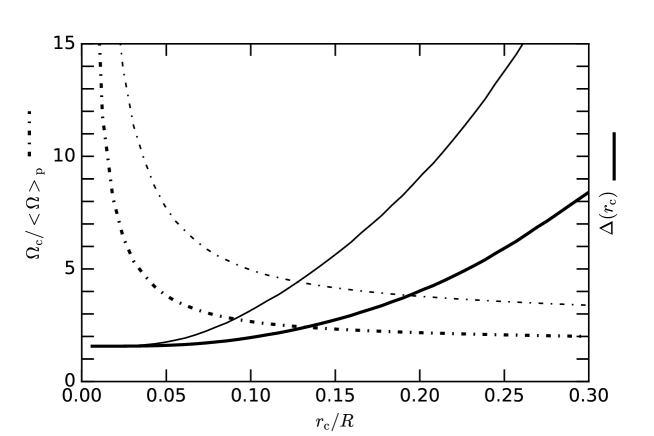
Figure 1: The dot-dashed curves are values of $\Omega_{\rm c}/<\Omega>_{\rm p}$ required to reproduce a g-mode rotational splitting $<\Omega>_{\rm g}$ from a presumed piecewise constant angular velocity $\Omega(r)=\Omega_{\rm c}\,$ where $r<r_{\rm c}$ and $\Omega(r)=<\Omega>_{\rm p}$ where $r>r_{\rm c}$, with $<\Omega>_{\rm p}/2\pi=433.5\,$nHz. The thinner curves were computed with $<\Omega>_{\rm g}/2\pi\,=1277\,$nHz, corresponding to assuming that g modes of degree 1 and 2 were detected by Fossat et al. (2017); the thicker curves correspond to assuming that only the lowest even-degree g modes were detected, implying $<\Omega>_{\rm g}/2\pi\,=789\,$nHz. The solid curves are the corresponding rms deviations $\Delta(r_{\rm c})$ from the GOLF p-mode rotational frequency splittings published by García et al. (2004) and Lazrek et al. (2004) of theoretical splittings resulting from the angular velocity $\Omega(r)$ in units of the standard errors in the splitting data. A similar plot assuming $\Omega(r)$ to exceed $<\Omega>_{\rm p}$ by a half-Gaussian with $r_{\rm c}$ defined as the radius at which the excess is half its central value is hardly different.

One interesting property of this result is that the three putative g-mode sequences (each with varying $n$) that are present at apparently observable amplitudes are associated with values of $s(l,m)$ that form, presumably coincidentally, an harmonic sequence. Yet perhaps the most startling aspect of the result is that, at least in the form presented by Fossat et al. (2017), it is contradicted by inferences of the Sun’s internal rotation obtained from direct measurements of rotational splitting of p modes. For example, Elsworth et al. (1995) inferred from BiSON data that the core of the Sun appears to be rotating no faster than the rest of the radiative interior, and probably even more slowly. And indeed, rotational splitting obtained from the GOLF data themselves (García et al., 2004; Lazrek et al., 2004) are consistent with that inference. Moreover, the rms deviation of the p-mode rotational splitting implied by the piecewise constant $\Omega$, with $r_{\rm c}=0.2R$, is $\Delta=8.9$ mean standard errors (in the rotational splitting data), whereas the deviation implied by uniform rotation is less than 1.6 standard errors. However, it cannot immediately be said that there is a genuine contradiction, because the p modes do not sense the very central regions of the Sun as much as do high-order g modes. It should be appreciated that no constraint on $r_{\rm c}$ has been established; a small very rapidly rotating core cannot be negated by direct p-mode seismology. The value of the core radius $r_{\rm c}$ adopted by Fossat et al. (2017) is quite arbitrary, so it behoves one to consider other values. In Figure 1 we plot against $r_{\rm c}/R$ the rms deviation $\Delta$ from the published GOLF data of the p-mode frequency splittings implied by the assumed piecewise constant $\Omega$, in units of the rms uncertainties in the observations, choosing $\Omega_{\rm c}(r_{\rm c})$ to maintain the value of $<\Omega>_{\rm g}\,$ claimed by Fossat et al. (2017). $\Omega_{\rm c}/\Omega_{0}$ is also plotted. The theoretical splittings were evaluated using rotational splitting kernels computed from Model S of Christensen-Dalsgaard et al. (1996). A similar plot assuming $\Omega(r)$ to exceed $\Omega_{0}$ by a half-Gaussian with $r_{\rm c}$ defined as the radius at which the excess is half its central value: $\Omega(r)=\Omega_{0}+(\Omega_{\rm c}-\Omega_{0}){\rm exp}[-({\rm ln}2)(r/r_{\rm c})^{2}]$ yields values for $\Omega_{\rm c}$ typically about 3% greater. Taking the claim by Fossat et al. at face value, the mean g-mode frequency mismatch from equation (17) is about 4 standard errors.

It seems that the rapidly rotating core would need to be quite small if a significant inconsistency is to be avoided. That would raise serious fluid dynamical issues, although it can be said that the shear layer between the two regimes, provided it were not too thin, could be dynamically stable at least to the Richardson criterion. But there is another obvious, and rather more disturbing, issue that needs first to be addressed, namely that odd-degree g modes should not be detectable in the p-mode spectrum. To that property we now turn our attention.

3 On the strength of the g-mode coupling

The p-mode frequency perturbations can be estimated from equation (11), using degenerate perturbation theory. The g-mode amplitude estimates reported in a second paper, by Fossat & Schmider (2018), imply that ${|[\cal R}_{\boldsymbol{u}}+(\delta{\cal K}-\omega^{2}\delta{\cal I})/2\omega]/{\cal I}\omega|$ is very small (of order $10^{-5}$); therefore the deviation of the eigenfunctions from individual functions of the form given by equations (5) and (6) is also very small. Kennedy et al. (1993) remarked that it had been shown that the integral $\delta{\cal K}-\omega^{2}\delta{\cal I}$ vanishes for density and pressure perturbations with spherical-harmonic dependence of odd degree (Gough, 1993), and concluded that g modes of odd degree cannot be detected from p-mode frequency changes. Formally, that result had been derived for structure perturbations in hydrostatic balance. However, it is straightforward to demonstrate that it holds also for any harmonic structure perturbation of odd degree, whether it be in hydrostatic balance or not, and also that the g-mode velocity contribution to the integral ${\cal R}_{\boldsymbol{u}}$ vanishes too (see Appendix A). Therefore the assumption that dipole g modes are responsible for the principal peak near $\nu_{1}$ in the rotational diagnostic is thrown into very serious doubt. One could, however, adopt the assumption that it is quadrupole and hexadecapole modes that are responsible for the three principal peaks. Applying the argument of Fossat et al. (2017), again recognizing the ambiguity of the signs of the splitting frequencies, then leads to a slower core rotation, but still substantially faster than the surrounding radiative envelope. In that case, $<\Omega>_{\rm g}/2\pi\,\,=789\pm 10$ nHz, and the rms deviation of the inferred splitting of the frequencies of ${\rm g}_{(l=2,m=1)}$ from $\nu_{1}$, ${\rm g}_{(l=4,m=2)}$ from $\nu_{2}$ and ${\rm g}_{(l=4,m=4)}$ from $\nu_{3}$, again when it is assumed that $r_{\rm c}=0.2R$, is 4.4 nHz, which is hardly different from the deviation according to the interpretation of Fossat et al. The rms p-mode misfit from the GOLF frequencies (García et al., 2004; Lazrek et al., 2004) is then $\Delta=4.0$ standard errors. The core rotation, and also the misfit to the p-mode rotational splitting frequencies, are plotted in Figure 1 against putative core radii $r_{\rm c}$ up to $0.3R$.

We add that, following Fossat et al. (2017), one might alternatively, and arguably more naturally, identify the largest (210 nHz) principal peak in the autocorrelation with the detectable (prograde) g modes of lowest degree and azimuthal order, namely $l=2,\,m=1$; that would imply a core rotating somewhat more slowly than the surrounding radiative interior, yielding $<\Omega_{\rm g}>/2\pi=394\,{\rm nHz}$, which is consistent with earlier inferences from BiSON p-mode rotational splitting frequencies (Elsworth et al., 1995; Chaplin et al., 1999). However, it leaves the other principal peaks, if they be significant, unexplained.

Another outcome of the undetectability of odd-degree g modes is that the argument by Fossat et al. (2017) in their §5 based on fitting a theoretical frequency distribution to the GOLF power spectrum as a means of justifying the detection of dipole g modes must evidently be suspect. In §9 here we have more to report about theoretical model fitting for the purpose of establishing, or even merely strengthening, a case for the existence of a proposed phenomenon.

Finally, we point out that in a second paper Fossat & Schmider (2018) estimate, again by model fitting, some amplitudes of the components of the frequency variations of the p-mode peaks induced by what they believe to be the gravest (lowest order $|n|$) of the g modes that they studied. From that information one can make a crude estimate of the g-mode amplitudes from equation (11), using expressions (A7), (A8) and (A9) to determine the coupling integrals. A precise evaluation cannot be made, because we do not know the relative amplitudes of the many p modes to which the g modes were coupled. If they were approximately equal, then the surface velocity amplitude of the quadrupole g mode $g_{36,l=2}$ would be of the order of 50 cm $\rm s^{-1}$; the uncertainty is comparable at least with the value. Nevertheless, this estimate, being seriously in excess of the upper bound estimated by the Phoebus collaboration (Appourchaux et al., 2010), sheds doubt on the fitting procedure.

4 The form of the p-mode signature

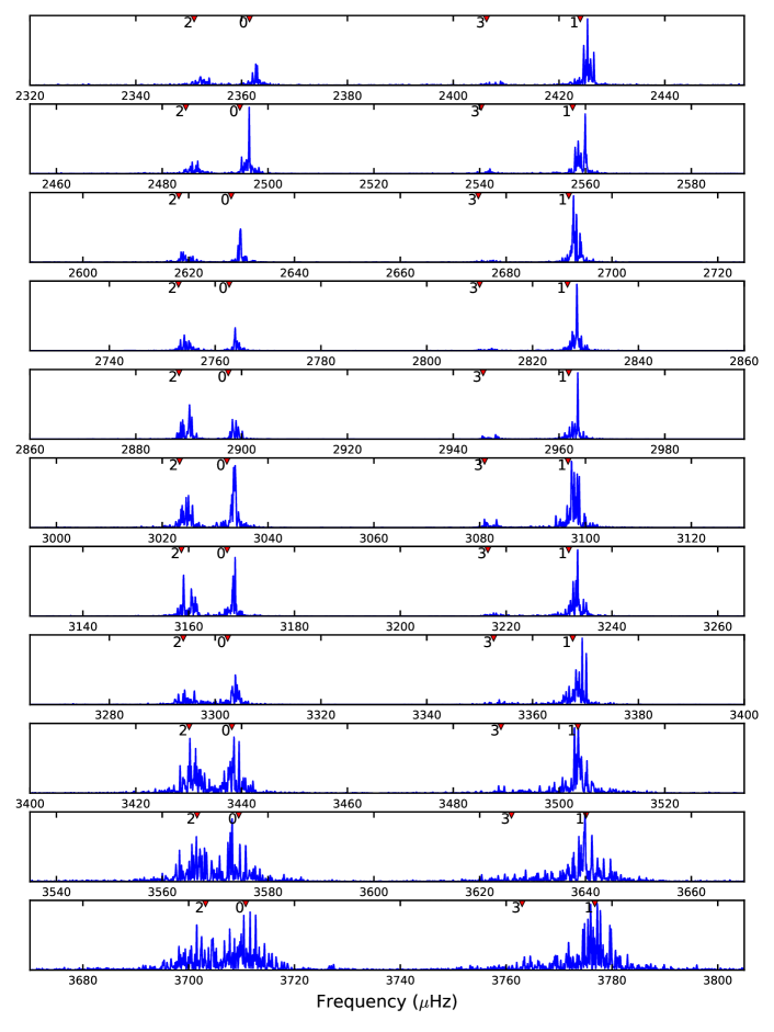
Figure B1: SOHO/GOLF echelle diagram showing stacked sections of the GOLF p-mode spectrum after Grec et al. (1983). Only the frequency range selected by Fossat et al. (2017) is shown. The data here is a 72 day interval of the GOLF data starting in 1996. To aid in identification the locations of the $l=0,1,2,3$ p-mode frequencies from Christensen-Dalsgaard et al. (1996) model S are shown as red triangles at the top of each row with the $l$ value label. Each row is scaled to the maximum power in that row. The effect of shorter lifetimes with increasing frequency is evident.

The low-degree p-mode spectrum is composed of contributions arising principally from the multiplet cyclic frequencies $\nu_{n,l}$ (where here $n$ denotes the order of the p mode) given approximately by equation (7), each of which, broadly speaking, is split by rotation (and further, but to a much lesser degree, by the presence of g modes and any other non-spherical perturbation, which for the moment we ignore) into singlets separated by $<\Omega_{\rm p}>/2\pi$. The so-called small (multiplet) separation $d_{n,l}:=\nu_{n,l}-\nu_{n-1,l+2}\simeq 2(2l+3)A_{\rm p}\nu_{0}^{2}/\nu_{n,l}$ cannot be resolved in a power spectrum of observations of 8 hr duration, and so each peak in the power spectrum is composed of a sum of modes of alternately odd and even degree. In view of the relative sensitivity of the whole-disc GOLF observations (e.g. Christensen-Dalsgaard & Gough, 1982), the major contributors to each peak are alternately $l=0$ and $l=2$, and $l=1$ and $l=3$, whose frequencies are separated by about 10 $\mu$Hz and 17 $\mu$Hz respectively. Stochastic variations of the amplitudes of those contributing components are the major source of the frequency variation of the spectral peaks, whose magnitudes are comparable with the frequency separations of the components. Those variations occur on timescales of typically a few days, the nominal lifetimes of the p modes. We illustrate in the Supporting Material (Figure B1) a typical resolved echelle spectrum in the frequency range adopted by Fossat et al. (2017), which displays, particularly at high frequency, the resulting spread of apparently resolved frequencies. In view of the low sensitivity of whole-disc Doppler observations to modes with $l=3$, the frequencies of the odd-degree peaks in the power spectrum result almost entirely from the apparent frequency variation of the dipole p modes, which is much smaller than the frequency variation of the even-degree peaks, whose principal contribution comes from the variation of the relative surface velocity amplitudes of the more widely spaced (in frequency) radial and quadrupole modes, producing frequency shifts of the p-mode peaks of amplitude about 4 $\mu$Hz. (Note that radial p-mode frequencies are unaffected by the necessarily nonradial g modes.) Superposed on these random frequency variations is a spectrum of phase-coherent g-mode-induced variations, which are of very much lower amplitude. However, most of the g modes are expected to maintain phase over a period comparable with or greater than the 16.5-year duration of the GOLF observations, so there can be hope of detecting them. Did Fossat et al. succeed in doing that?

5 Examination of the GOLF data analysis

Schunker et al. (2018) have already essentially reproduced and extended some of the results reported by Fossat et al. (2017). We first sought to do likewise, following Schunker et al. where the procedure was not described adequately by Fossat et al. At our disposal were two 16.5-year (1996-04-11 through 2012-10-05) whole-disc velocity observations obtained by the GOLF instrument, one averaged with a 60-second cadence, the other, which were the data of whose analysis Fossat et al. report, with a cadence of 80 seconds. We used 60 second GOLF data obtained from the SOHO data archive and 80 second cadence data provided by E. Fossat (personal communication, 2018) to match the same calibration used by Fossat et al. (2017). Each data set was divided into 8-hour overlapping segments whose start times were separated by 4 hours. Acceptable segments, namely those having duty cycles exceeding $90\%$, were zero-padded to $10^{6}$ seconds, and power spectra were computed. The segments of those spectra between 2.32 mHz and 3.74 mHz were extracted and divided by a Gaussian envelope function with standard deviation 0.39 mHz, centered at 3.22 mHz, and then zero-padded to produce a frequency series in the range 0 – 125 mHz. The spectrum of this series was then computed to produce a ‘period spectrum’. The dominant peak in this spectrum is usually near 14800 seconds. This period is associated with half the large p-mode separation, about $(67.54~{}\mu{\rm Hz})^{-1}\simeq 14800~{}{\rm s}$. The period for each 8-hour segment was obtained by fitting to it an inverted parabola of total width 1600 s, as did Fossat et al. This process produced a time series of 36132 possible values for the 80-second data and 36131 for 60-second data. In a two-step process first, ignoring times where insufficient data were available, the mean was removed, then times exceeding $\pm 240s$ were removed, then the mean of the remaining 34095 useful representations of travel-time measurements for the 80-second data (34155 for the 60 second data) was removed and outliers and times with no data were set to zero. The standard deviation for these two series is 52.0 and 51.1 for the 80 and 60 second series respectively. The power spectra of these 4-hour-cadence series were smoothed with a six-pixel-wide boxcar, with weights (0.5,1,1,1,1,1,0.5), and the autocorrelation curves were finally obtained. The outcome from the two data sets are depicted in Figure 2, which is the analog of Figure 10 of Fossat et al. The frequency lags $\nu_{k}$ = 210 nHz, 630 nHz and 1260 nHz, claimed to be g-mode rotational splitting frequencies, are indicated by the vertical dashed lines. Panel (a) was obtained from the data with 80-second cadence; peaks at the frequencies $\nu_{k}$ are clearly evident, although the peak at $\nu_{3}$ is not as high as some of those that follow. Panel (b) was obtained from the data with 60-second cadence; interestingly, not all the frequency lags $\nu_{k}$ correspond to prominent peaks. The standard deviation $\sigma$ about the mean is the same, about 0.015, for both data sets.

It is disturbing that the two different averaging intervals (60 s and 80 s) of the same GOLF data set yield substantially different autocorrelation functions, particularly because the highest principal peak in one is hardly outstanding in the other. We have repeated some of the tests carried out by Schunker et al. (2018), such as the sensitivity of the results to: the cadence of the power spectra of the GOLF data segments (4 hours in the case of the analysis by Fossat et al.); the method of estimating the time interval of the p-mode peak in the power spectrum of those power spectra, which represents the inverse of half the large frequency spacing, approximately twice the sound travel time through a diameter of the solar interior; the method of smoothing the power spectrum of those time intervals; and ignoring a short segment of the GOLF time series, thereby introducing an offset in the segmentation of the data. We are in broad agreement with the earlier work.

f2a.epsf2b.eps

Figure 2: Autocorrelation of power spectrum of p-mode peaks in power spectrum of power spectrum of GOLF data: (a) from 80-second cadence, (b) from 60-second cadence. The vertical dashed lines locate the frequencies 210 nHz, 630 nHz and 1260 nHz claimed by Fossat et al. (2017) to be g-mode rotational splitting frequencies. The horizontal solid, dashed, dotted reference lines show correlation levels 0.0, the mean from 0.023 to 3.5 $\mu$Hz, and one $\sigma$ above the mean respectively.

6 MDI and HMI data

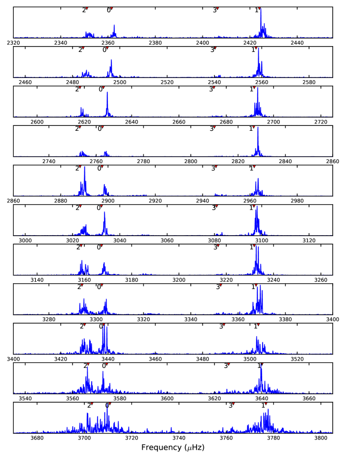
Figure B2: SOHO/MDI $l=0$ echelle diagram for the same interval as B1. The similarity of this figure and B1 shows that using the $l=0$ spherical harmonic for MDI and other instruments providing data as spherical harmonics provides similar mode sampling as the unimaged GOLF data.

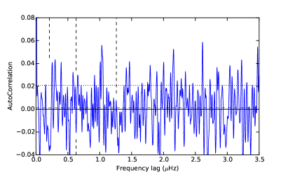
Figure B3: SOHO/MDI 60-second data for the 14.6-year interval from 1996-04-30 through 2010-12-01 (Scherrer et al. (1995)) processed the same as in Figure 10 of Fossat et al. (2017) and Figure 2 here. The vertical and horizontal lines are the same as in Figure 2.

Even given the uncertainties described in the preceding sections, we considered it to be worthwhile to use the same procedure from Fossat et al. (2017) as described above to examine other datasets with comparable sensitivity to p modes and comparable intervals of available data (see Supporting Material, Appendix B) for a list of data sources used. We started with SOHO/MDI (Scherrer et al., 1995) data for the 15.5 year interval 1996-05-01 through 2011.04.11 which is all but the final year examined by Fossat et al. (2017). MDI data processed for use in helioseismology studies are available for spherical harmonic projections of degree 0 through 300. The best match to the GOLF view of the Sun is to use the time series for degree 0, which is available as described in Supporting Material for section 6. Inspection of an echelle diagram similar to Figure B1, available in the Supporting Material as Figure B2, provides confirmation that MDI sees $l$ = 0 through 3 with relative sensitivity similar to GOLF. MDI observed solar photospheric motions at a 60-second cadence, and has nearly as complete a coverage as GOLF. The MDI version of Figure 10 of Fossat et al. (2017), shown in Supporting Material as Figure B3, has a set of peaks superficially similar to those of the GOLF Figure 10, but none of them are near the three identified peaks seen in the GOLF figure. It is interesting that the standard deviation of the semi-large-separation times for MDI is 58.8 seconds, close to the cadence of 60 seconds, for the available 30149 times in the span containing 31967 possible measurements.

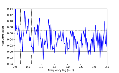
Figure B4: SDO/HMI 45-second data for the 8.5-year interval from 2010-04-30 through 2018-10-20 (Schou et al. (2012)) processed the same as in Figure 10 of Fossat et al. (2017) and Figure 2 here.

We next examined the available 8.5-year interval from 2010-04-30 through 2018-10-20 from SDO/HMI (Schou et al. (2012). HMI is a higher-resolution version of MDI, but with a cadence of 45 seconds and fewer data gaps. We applied the same procedure as described above to analyse the observations for degree 0. For HMI there are 17996 of a possible 18143 semi-large-separation measurements with the 4-hour cadence, the coverage being 99% compared to 94% for MDI and GOLF, and the standard deviation of the set of times is less at 42.9 seconds. There is a peak in the HMI version of Figure 10 near 1260 nHz (Figure B4), but it is only the fourth highest, and there are no substantial peaks at 210 nHz nor 630 nHz. It is possible that effects of solar activity may have leaked into the analysis, or that the putative g-mode signal itself varies with time. We can compare the HMI result with that from GOLF by using data from the same interval.

GOLF observations did not cease in 2012, and Appourchaux et al. (2018) have recently prepared a newly recalibrated 22-year GOLF dataset, now available directly from the GOLF project at https://www.ias.u-psud.fr/golf for Level 2 data. These GOLF data are available at a 20-second cadence, allowing comparison of the 60-second and 80-second cadence versions of Figure 10 with the same calibration. Supporting Material Figure B5 (a) and (b) show the results obtained in the interval 2010-04-30 through 2018-04-30. The standard deviations of the times are 66.6 and 65.2 seconds for 80- and 60-second cadences respectively, with 96% coverage. Fossat et al. (2017) found the peaks of interest in subsets of the GOLF data so one might have expected to see some similar pattern in the HMI data which shows a narrower distribution in the half-separation times than the GOLF data. We have included ”Figure 10” analyses of the Appourchaux et al. (2018) 80-second and 60-second data for the earlier 1996 to 2012 interval for comparison to Figure 2 and Fossat et al. (2017) Figure 10. We see that the key 210 nHz peak is clear in this 80-second data as it was in the original data but not in the 60-second data. In this case the same calibration of the GOLF data was used to generate the 80- and 60- second tests.

7 Analysis of other observations

We have carried out similar analyses of other observations, namely by GONG (Global Oscillation Network Group), by the BiSON (Birmingham Solar Oscillations Network: Davies et al. (2014) and Hale et al. (2016) ), and by VIRGO/LOI (Variability of solar IRradiance and Gravity Oscillations Luminosity Oscillations Imager) on the SOHO spacecraft with broadly similar results (Figures B7, B8, and B9 respectively. In particular, the autocorrelations analogous to Figure 10 of Fossat et al. (2017) and Figure 2 here are superficially similar. However, the principal peaks are not at the same frequency lags. Evidently, the procedure is not robust. Further details are presented in the Supporting Material.

8 Offset start times

The effect of offsetting the start times of the data analysed perhaps provides some clue to interpreting the principal autocorrelation peaks evident in Figure 2. In Figure 3 we plot the heights of those peaks as a function of the offset. They all drop sharply as the offset increases from zero, and remain low until the offset approaches the 4-hour g-mode cadence. The autocorrelations at the offset of the g-mode cadence, and at any moderate integral multiple of it, are hardly distinguishable, because each 4-hour offset simply reduces the length of the 16.5-year data set by just one part in about 36000. However, a non-integral offset changes the phase of the data segment relative to terrestrial time, the effect of which is to reduce the autocorrelation. So maybe the autocorrelation peaks result from perturbations in the spacecraft, such as voltage glitches caused by transmitting data to Earth, whose occurrences are linked to terrestrial time. We have searched for a 210 nHz frequency and its harmonics in those spacecraft procedures of which we are aware, and have found none. Nevertheless, a terrestrially controlled process on SoHO, either directly or indirectly related to GOLF, but not to MDI or VIRGO, remains a candidate for causing the autocorrelation peaks. It is interesting that Fossat et al. chose their g-mode cadence to be 4 hours, which is an integral factor of a day; as Schunker et al. (2018) have pointed out, the principal autocorrelation peaks are smaller at different cadences. That is the case even for a cadence of 3 hours, which is also an integral factor of a day. We have no explanation for that behaviour.

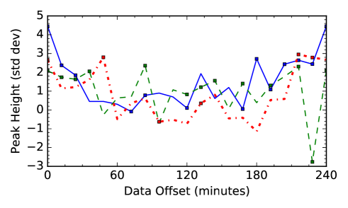
Figure 3: Heights of the purported g-mode peaks with respect to the offset (in seconds) of the start time of the portion of GOLF data analysed. Plotted are the greatest values of the autocorrelation, such as that in Figure 2 (but here in units of the standard deviation $\sigma$ in the entire frequency range 0 – 3500 nHz), in a frequency window $\pm 10$ nHz (the resolution width) about the frequencies $\nu_{k}$. They are joined by straight lines: continuous between peaks at about $\nu_{1}=210\,{\rm nHz}$, dashed about $\nu_{2}=630\,{\rm nHz}$, and dot-dashed about $\nu_{3}=1260\,{\rm nHz}$. The symbols mark peaks in the autocorrelation; where there is no symbol, there is no peak in the frequency range considered, the value plotted then being the autocorrelation at one of the limits of the window.

9 Theoretical-model fitting

Fossat and his colleagues carried out two model-fitting procedures to justify their interpretation of their analysis of the GOLF data. The first, by Fossat et al. (2017), was a two-dimensional fit with respect to uniform asymptotic multiplet dipole period spacing $\sqrt{2}P_{0}$ according to the leading term on the right-hand side of equation (9) and uniform rotational frequency spitting, according to equation (16). We note, in passing, that the dipole assumption is in conflict with the expectation that g modes of only even degree are accessible. The other procedure, reported in the second paper (Fossat & Schmider, 2018), was a simpler, one-dimensional, degree-by-degree fit to the GOLF p-mode power spectrum of the approximate g-mode frequency formula (obtainable from equations (9) and (16)):

$$\nu_{n,l,m}\simeq\frac{L}{(|n|+l/2+\alpha_{\rm g})P_{0}}+\frac{m}{2\pi}(1-L^{-2})<\Omega_{\rm g}>\,,$$ (18)

designed to detect rotational splitting of modes of degree $l=3$ and $l=4$. Here we address only the second procedure.

Once again, odd values of the degree $l$ were considered by Fossat and Schmider, which should be hardly detectable by p modes. The fittings were accomplished by cross-correlating peaks at frequencies given by equation (18) with the power spectrum of the GOLF p-mode peaks, adjusting not only the values of the parameters $P_{0}$, $\alpha_{\rm g}$, $<\Omega_{\rm g}>$, and the relative amplitudes of the modes, but also the frequency range adopted for the cross-correlation, in order to maximize the height of the zero-lag peak. In the expectation that the g-mode frequency splitting is symmetrical with respect to azimuthal order $m$, the cross-correlation was symmetrized against zero lag to ease the optimization.

Such a procedure can surely be used to fine tune a formula for a signal whose source is assured. However, we doubt that it can be used to prove the existence of such a source. To support our opinion, we have carried out a broadly similar analysis for a theoretical asymptotic spectrum of combined quadrupole and hexadecapole g modes in the frequency range 4–35 $\mu$Hz, selecting the relative amplitudes of the modes in such as way as to enhance both the zero lag and two ‘split’ components at $\pm 210$ nHz. An example of the symmetrized cross-correlation is depicted in Figure 4. The frequency splitting in equation (18) was not included: it was not necessary because each entry in the power spectrum against which the theoretical spectrum was cross-correlated was random, drawn from a Boltzmann distribution, and so contained no information whatever about rotational splitting, or even g-mode multiplet frequencies. Moreover, we did not even adjust the other parameters in the right-hand side of equation (18) to enhance the fit. As in Figure 2 of Fossat & Schmider (2018), the height of the peak at zero lag above the mean exceeds 10.5$\sigma$, where $\sigma$ is the standard deviation of the cross-correlation, and the height of the ‘splitting’ peaks exceeds the 4.5$\sigma$. To assess the significance of that result, we carried out 20 such analyses with different independently computed realizations of the Boltzmann distribution. Of those, $10\%$ had a zero-lag height above 10.5$\sigma$, $45\%$ above 9$\sigma$ and $90\%$ above 8$\sigma$; the heights of the ‘splitting’ peaks exceeded the 4.5$\sigma$ achieved by Fossat and Schmider in all cases. We accept that our amplitude-adjustment procedure may have been different from that adopted by Fossat and Schmider (who did not report how their amplitudes were chosen), but we offer this exercise merely to warn against hasty inferences, not only that discussed here in support of the existence of rotationally split g-modes of degrees 3 and 4, but also the two-dimensional fitting reported earlier by Fossat et al. (2017).

Of course, from the point of view of this exercise the choice of a 210 nHz frequency lag for the cross-correlation of the theoretical spectrum with the random artificial power spectrum was arbitrary, and we could equally well have obtained similar results with a different lag. Accordingly, we carried out the same exercise with the power spectrum of the GOLF data (obtained from the 80-s binning), attempting to reproduce peaks at lags other than frequencies $\nu_{k}$ of the principal peaks. We found it to be significantly more difficult to achieve results as clean as those obtained from the random power spectra, such as that illustrated in Figure 4. We therefore conclude that the frequencies of the p-mode peaks obtained from the GOLF data are not random. However, we have no explanation for what the non-randomness might be.

f4a.epsf4b.eps

Figure 4: Cross-correlation of an artificial g-mode power spectrum with a reference power spectrum: (a) Figure 1 of Fossat & Schmider (2018), whose reference is the large-separation spectrum of 80-second GOLF data, (b) the reference spectrum is random, each point having been drawn from a Boltzmann distribution. (Part (a) reproduced with permission from Astronomy & Astrophysics, ©ESO.)

10 Concluding remarks

Our investigation has led us to doubt the report by Fossat et al. (2017) of a detection of solar g modes via their interaction with p modes, and that a measurement of rotational splitting implies that the core of the Sun is rotating rapidly. The exact value of the angular velocity inferred at the centre of the Sun depends on an assumption of the variation with radius – Fossat et al. assume that the region of rapid rotation extends to 20 per cent of the solar radius, from which they obtain a rotation rate 4.8 times that of the surrounding envelope – but that detail is not our major concern. Aside from the near inconsistency with direct inferences from p-mode rotational splitting obtained from the same GOLF data by García et al. (2004) and Lazrek et al. (2004), and the reported g-mode amplitudes appearing to exceed the upper bound reported by the Phoebus group (Appourchaux et al., 2010), the unconfirmed interpretation of the dominant modulation of the p-mode oscillations being due to dipole g modes is at odds with the property that odd-degree (static or slowly varying) spherically harmonic perturbations to the background state of the star do not modify p-mode frequencies in leading order. Our neglect in the analysis we present explicitly here of the latitudinal variation of the angular velocity in the convection zone, and of the slow temporal variation of the g modes compared to the p modes (e.g Lavely & Ritzwoller, 1992; Hanasoge et al., 2017), makes no material difference to that conclusion. Fossat et al. appear to favour the assumption that the coupling, if it is detectable, is to g modes of lowest degree. Therefore it is perhaps more natural in the first instance to adopt a more simplistic presumption: that the dominant peak in their autocorrelation arises from quadrupole modes. That does not explain the other peaks. However, we demonstrate here that those other peaks, and even the dominant peak, are not robustly determined. Interestingly, the simplistic assumption implies that the Sun’s core is rotating somewhat more slowly than the surrounding radiative envelope, which would be consistent with earlier findings from BiSON (Elsworth et al., 1995).

Notwithstanding these immediate reactions, we have been led to investigate the analysis of the GOLF data more thoroughly, seeking to establish how robust are the conclusions of Fossat et al. (2017) to modifications of the procedure adopted. In agreement with a recent investigation by Schunker et al. (2018), and noting that the record lengths and the cadence of the segmented data analysed by Fossat et al. are small factors of a terrestrial day, we have found that the dominance of the autocorrelation peaks depend critically on universal time. We are also suspicious that the frequencies of the principal autocorrelation peaks, despite their apparent disparate physical origins, form an harmonic sequence. Shifting the start times of the data segments by a small non-integral factor of a day reduces, or obliterates, the correlation, as does similarly changing the cadence. Moreover, we find from analysing corresponding seismic data from MDI, HMI, VIRGO, GONG and BiSON that although superficially similar autocorrelations emerge, the frequencies of the peaks do not coincide.

We therefore surmise that the GOLF data have been influenced in some way by terrestrial processes that do not influence the other instruments in the same manner, and that the conclusions of Fossat et al. are premature.

Note added in revision: Appourchaux & Corbard (2019) have performed similar tests and found similar results.

11 Acknowledgments

We are grateful to Todd Hoeksema and Thierry Appourchaux for constructive discussion and Eric Fossat for providing the 80 second data he used. We also thank the SOHO GOLF and VIRGO/LOI teams for making their data available as per the SOHO data access policy, and the Birmingham Solar-Oscillations Network group for access to the BiSON data. This work utilizes data obtained by the Global Oscillation Network Group (GONG) program, managed by the National Solar Observatory, which is operated by AURA, Inc. under a cooperative agreement with the National Science Foundation. The data were acquired by instruments operated by the Big Bear Solar Observatory, High Altitude Observatory, Learmonth Solar Observatory, Udaipur Solar Observatory, Instituto de Astrofísica de Canarias, and Cerro Tololo Interamerican Observatory. We acknowledge support by HMI NASA contract NAS5-02139.

Appendix A g-mode velocity contribution

As explained in the introduction, on the timescale of the diagnosing p modes the temporal variation of the g modes can be ignored, permitting instantaneous p-mode frequencies $\omega$ to be envisaged. These are determined by equations (1) - (4) after linearization about the basic nonrotating equilibrium state of the star with respect to the velocity $\boldsymbol{v}$ and the perturbed structure $\Delta\rho$, $\Delta p$ resulting from the g modes. The former is separated into pure (axisymmetric) rotation $\boldsymbol{\Omega}$ and the (real) g-mode velocity ${\boldsymbol{u}}$, and can be written

$${\boldsymbol{v}}=:{\boldsymbol{\Omega}}\times{\boldsymbol{r}}+\Sigma_{\rm order}\Sigma_{l}{\boldsymbol{u}}_{l}\,,$$ (A1)

where

$${\boldsymbol{u}_{l}}=\Sigma_{m=-l}^{l}A_{l,m}{\boldsymbol{u}_{l,m}}$$ (A2)

is the g-mode velocity component of degree $l$, with azimuthal component amplitudes $A_{l,m}$, in which

$$2\,{\boldsymbol{u}_{l,m}}=\left(W_{l}(r)P^{m}_{l},\frac{U_{l}(r)}{L}\frac{{\rm d}P^{m}_{l}}{{\rm d}\theta},\frac{{\rm i}mU_{l}(r)}{L{\rm sin}\theta}P^{m}_{l}\right){\rm e}^{{\rm i}m\phi}\,+{\rm c.c.}\,,$$ (A3)

$L=\sqrt{(}l(l+1))$ and c.c. denotes complex conjugate. For simplicity and without loss of generality, we take $W_{l}(r)$ and $U_{l}(r)$ to be real. The outer sum in equation (A1) is over all orders of the g modes; the amplitude functions $(W_{l},U_{l})$ are presumed to be normalized to unit inertia for each $l$. To avoid unnecessary notational complication, we have omitted labels indicating mode order from $W_{l}\,,U_{l}$ and the amplitudes $A_{l,m}$. The associated g-mode-induced pressure and density perturbation eigenfunctions, $\Delta p(r)P^{m}_{l}({\rm cos}\theta)$ and $\Delta\rho(r)P^{m}_{l}({\rm cos}\theta)$, are related to the velocity eigenfunctions by the (adiabatic) oscillation equations (e.g. Unno et al., 1989):

$$\frac{{\rm d}\Delta p}{{\rm d}r}+\frac{g}{c^{2}}\Delta p+(N^{2}-\omega_{\rm g}^{2})\omega_{g}^{-1}\rho W=0,$$ (A4)

$$\Delta\rho=c^{-2}\Delta p+g^{-1}N^{2}\omega_{\rm g}^{-1}\rho W$$ (A5)

in an obvious notation; $\omega_{\rm g}$ is the g-mode frequency.

The g-mode-induced perturbations to p-mode eigenfrequencies are given by equation (11). Following normal degenerate perturbation theory, to leading order in the g-mode-induced perturbations, the resulting p modes of degree $\lambda$ can be represented as a sum over azimuthal order $\mu$ of all the zero-order eigenfunctions of degree $\lambda$ (and given order $n$) in the integrals in equation (11):

$$\boldsymbol{\xi}_{n,\lambda,\alpha}=\Sigma_{\mu}c^{\alpha}_{n,\lambda,\mu}\boldsymbol{\xi}_{n,\lambda,\mu}\,;\;\;\;\psi_{n,\lambda,\alpha}=\Sigma_{\mu}c^{\alpha}_{n,\lambda,\mu}\psi_{n,\lambda,\mu}\,,$$ (A6)

where $\alpha$ labels the perturbed eigenmodes. The coefficients $c^{\alpha}_{n,\lambda,\mu}$ are determined by substituting this sum into equation (11). We do not present the entire analysis here, but merely inspect the contributions to the coupling integrals (2)-(4) from a pair of p modes and a single g mode. Beginning with the structure perturbations, we record that

$$\delta_{\lambda,\mu,\mu^{\prime},l,m}{\cal K}=\int_{\cal V}\big{(}\gamma\chi^{\prime*}\chi\Delta_{l,m}p+(\xi^{\prime*}\chi+\xi\chi^{\prime*})\left[\frac{g}{c^{2}}\Delta_{l,m}p+(N^{2}-\omega_{\rm g}^{2})\omega_{\rm g}^{-1}\rho W_{l,m}\right]$$

$$+\frac{\rm d}{{\rm d}r}(g\xi^{\prime*}\xi)\Delta_{l,m}\rho\big{)}P^{m}_{l}P^{\mu}_{\lambda}P^{\mu^{\prime}}_{\lambda}{\rm e}^{{\rm i}(\mu-\mu^{\prime}+m)\phi}{\rm d}V\,,$$ (A7)

$$\delta_{\lambda,\mu,\mu^{\prime},m}{\cal I}=\int_{\cal V}(\xi^{\prime*}\xi+\eta^{\prime*}\eta)\Delta_{l,m}\rho P^{m}_{l}P^{\mu}_{\lambda}P^{\mu^{\prime}}_{\lambda}{\rm e}^{{\rm i}(\mu-\mu^{\prime}+m)\phi}{\rm d}V\,,$$ (A8)

in an obvious notation, where $\chi={\rm div}\boldsymbol{\xi}$ and $\gamma$ is the first adiabatic exponent; the asterisk denotes complex conjugate. The integrand has $P^{m}_{l}P^{\mu}_{\lambda}P^{\mu^{\prime}}_{\lambda}{\rm exp}({\rm i}(\mu-\mu^{\prime}+m)\phi]$ as a factor. Noting that there is another contribution $\delta_{\lambda,\mu,\mu^{\prime},l,-m}{\cal K}$ to $\delta{\cal K}$, it follows that at least one of $\mu-\mu^{\prime}\pm m$ must vanish for the sum of the two integrals not to vanish, from which it follows that $\mu-\mu^{\prime}+m$ is even. Note also that $P^{\mu}_{\lambda}$ is an odd or even function of ${\rm cos}\theta$ according to whether $\lambda+\mu$ is odd or even. Therefore $P^{m}_{l}P^{\mu}_{\lambda}P^{\mu^{\prime}}_{\lambda}$ is odd or even according to whether $l$ is odd or even, because $m+\mu+\mu^{\prime}$ is even. Hence the integrals vanish if $l$ is odd.

Analysis of the advection integral ${\cal R}_{\boldsymbol{u}}$ is algebraically more complicated, but is otherwise essentially the same. The component of the integrand analogous to the structure component (A7), omitting subscripts to the oscillation eigenfunctions on the right-hand side, is given by

$$\boldsymbol{\xi}^{*\mu^{\prime}}_{\lambda}.({\boldsymbol{u}_{l,m}}.\nabla)\boldsymbol{\xi}^{\mu}_{\lambda}=\big{(}\big{(}(W\frac{{\rm d}\xi}{{\rm d}r}-\frac{m\mu U(\xi-\Lambda^{-1}\eta)}{Lr{\rm sin}^{2}\theta})\xi^{\prime*}+(\frac{\mu\mu^{\prime}}{\Lambda^{2}{\rm sin}^{2}\theta}W\frac{{\rm d}\eta}{{\rm d}r}+\frac{m\mu^{\prime}}{L\Lambda r{\rm sin}^{2}\theta}U(\xi-\frac{\mu^{2}}{L\Lambda{\rm sin}^{2}\theta}\eta))\eta^{\prime*}\big{)}P^{m}_{l}P^{\mu}_{\lambda}P^{\mu^{\prime}}_{\lambda}$$

$$+\frac{m{\rm cos}\theta\eta\eta^{\prime*}}{L\Lambda^{2}r{\rm sin}^{3}\theta}UP^{m}_{l}(\mu P^{\mu}_{\lambda}\frac{{\rm d^{2}}P^{\mu}_{\lambda}}{{\rm d}\theta^{2}}+\mu^{\prime}P^{\mu^{\prime}}_{\lambda}\frac{{\rm d}P^{\mu}_{\lambda}}{{\rm d}\theta})+\frac{\mu\mu^{\prime}\eta\eta^{\prime*}}{L\Lambda^{2}r{\rm sin}^{2}\theta}U\frac{{\rm d}P^{m}_{l}}{{\rm d}\theta}(\frac{{\rm d}P^{\mu}_{\lambda}}{{\rm d}\theta}-{\rm cot}\theta\,P^{\mu}_{\lambda})P^{\mu^{\prime}}_{\lambda}$$

$$+\Lambda^{-2}(W\frac{{\rm d}\eta}{{\rm d}r}-\frac{m\mu\eta U}{\Lambda r{\rm sin}^{2}\theta})\eta^{\prime*}P^{m}_{l}\frac{{\rm d}P^{\mu}_{\lambda}}{{\rm d}\theta}\frac{{\rm d}P^{\mu^{\prime}}_{\lambda}}{{\rm d}\theta}+\frac{1}{Lr}(\xi-\Lambda^{-1}\eta)\xi^{\prime*}U\frac{{\rm d}P^{m}_{l}}{{\rm d}\theta}\frac{{\rm d}P^{\mu}_{\lambda}}{{\rm d}\theta}P^{\mu^{\prime}}_{\lambda}+\frac{\xi\eta^{\prime*}}{L\Lambda r}U\frac{{\rm d}P^{m}_{l}}{{\rm d}\theta}P^{\mu}_{\lambda}\frac{{\rm d}P^{\mu^{\prime}}_{\lambda}}{{\rm d}\theta}$$

$$+\frac{\eta\eta^{\prime*}}{L\Lambda^{2}r}U\frac{{\rm d}P^{m}_{l}}{{\rm d}\theta}\frac{{\rm d^{2}}P^{\mu}_{\lambda}}{{\rm d}\theta^{2}}\frac{{\rm d}P^{\mu^{\prime}}_{\lambda}}{{\rm d}\theta}\big{)}{\rm e}^{{\rm i}(\mu-\mu^{\prime}+m)\phi}\,,$$ (A9)

in which $\xi$ and $\eta$ represent components of the displacement eigenfunction of the p-mode of degree $\lambda$ (and order $n$) and azimuthal order $\mu$, and $\chi$ its divergence, and $\xi^{\prime}$, $\eta^{\prime}$ and $\chi^{\prime}$ represent the corresponding mode of azimuthal order $\mu^{\prime}$; also $\Lambda=\sqrt{(}\lambda(\lambda+1))$. Noting that the $\theta$ derivative of an odd function of ${\rm cos}\theta$ is even, and vice versa, it is evident that all the terms in expression (A9) have the same parity as $P^{m}_{l}P^{\mu}_{\lambda}P^{\mu^{\prime}}_{\lambda}$. Consequently the argument in the previous paragraph applies here too.

More directly, expression (A9) is real, which renders ${\cal R}_{\boldsymbol{u}}$ purely imaginary. Therefore advection by the g-mode flow, to first order, does not influence the real part of the p-mode frequencies. This comes about because, unlike rotational flow, the essentially hydrostatic g-mode stream lines are all closed, and the local p-mode Doppler shifts cancel, as is the case also for meridional circulation (e.g Gough & Hindman, 2010).

Therefore, taking all the contributions to the p-mode frequency perturbations into account, it follows that g modes of only even degree $l$ can influence the p-mode frequencies to leading order in the perturbations.

Appendix B Supporting Material

The following pages will consitute the Supporting Material.

The figures are the backup for statements about the Fossat et al. (2017) Figure 10 processing applied to additional long duration helioseismic datasets including GONG, VIRGO/LOI, BiSON. Also figures that support the use of SDO/HMI data from the interval after the end of the Fossat et al. 2017 interval and ’echelle’ format figures that support the use of l$l=0$ for MDI, LOI, HMI, and GONG where the data is available in spherical harmonics versus data collected from instruments that observer the Sun as a star with no spatial resolution namely BiSON and GOLF.

The data sources used for the analyses shown are below.

1. GOLF 60 second data originally from the SOHO archive is now available from http://www.ias.u-psud.fr/golf/assets/data/GOLF_velocity_series_mean_pm1_pm2.fits.gz,

2. GOLF 80 second data used in Fossat et al. (2017) is now found at https://www.ias.u-psud.fr/golf/assets/data/GOLF_series_Fossat_et_al.fits  data starts at 0:00:30 (T.A.I.) on April 11th 1996,

3. GOLF newer calibration 20 second data from Appourchaux et al. (2018) is now found at https://www.ias.u-psud.fr/golf/assets/data/GOLF_22y_MEAN.fits,

4. MDI data is from the JSOC export tool at http://jsoc.stanford.edu/ajax/exportdata.html?ds=mdi.vw_V_sht_gf_72d[1996.05.01_TAI-2011.02.12_TAI][0][0][103680]&limit=none,

5. HMI data is from the JSOC export tool at http://jsoc.stanford.edu/ajax/exportdata.html?ds=hmi.V_sht_gf_72d[2010.04.30_TAI-2018.10.21_TAI][0][0][138240]&limit=none,

6. GONG data is from https://gong2.nso.edu/archive/patch.pl?menutype=t for for $l=0$ for GONG months 1 through 225 useing start date 950507,

7. LOI $l=0$ data is from Thierry Appourchaux on 10 November 2017 and is available from him or Phil Scherrer on request,

8. BISON data is from https://edata.bham.ac.uk/59/, https://doi.org/10.25500/eData.bham.00000059 (catalog doi:10.25500/eData.bham.00000059)

The software used to generate these figures can be found in the Stanford Digital Repository at https://purl.stanford.edu/gt602xp9455

SM6-4a.epsSM6-4b.eps

Figure B5: GOLF data from Appourchaux et al. (2018) for the interval 2010.04-30 through 2018-04-30 for (a) 80-second and (b) 60-second averages of the available 20-second data, processed the same as in Figure 10 of Fossat et al. (2017) and Figure 2 here for comparison to Figure B4 HMI analysis. We note that the peaks seen in the 1996 to 2011 80-second data in both the Fossat et al. (2017) Figure 10 and Appourchaux et al. (2018) calibrations as in Figure 2 are absent in this later interval.

SM6-5a.epsSM6-5b.eps

Figure B6: GOLF data using 80 and 60 second averges of the 20-second data from Appourchaux et al. (2018) in the same format as Figure B5 but for the earlier 1996 to 2012 interval. As in Figure 2 here which used data from an earlier GOLF calibration the 210 nHz peaks are somewhat more visible in the 80-second sampling.

Figure B7: GONG 60-second data processed the same as in Figure 10 of Fossat et al. (2017) and Figure 2 here. The 3 peaks at 210, 630, and 1260 nHz are not significant.

Figure B8: BiSON 40-second data processed the same as in Figure 10 of Fossat et al. (2017) and Figure 2 here. The 3 peaks at 210, 630, and 1260 nHz are not significant.

Figure B9: SOHO/VIRGO/LOI 60-second data processed the same as in Figure 10 of Fossat et al. (2017) and Figure 2 here. The 3 peaks at 210, 630, and 1260 nHz are not significant.

References

- Appourchaux et al. (2018) Appourchaux, T., Boumier, P., Leibacher, J. W., & Corbard, T. 2018, A&A, 617, A108
- Appourchaux & Corbard (2019) Appourchaux, T., & Corbard, T. 2019, Submitted to A&A
- Appourchaux et al. (2010) Appourchaux, T., Belkacem, K., Broomhall, A.-M., et al. 2010, A&A Rev., 18, 197
- Chaplin et al. (1999) Chaplin, W. J., Christensen-Dalsgaard, J., Elsworth, Y., et al. 1999, MNRAS, 308, 405
- Christensen-Dalsgaard & Gough (1982) Christensen-Dalsgaard, J., & Gough, D. O. 1982, MNRAS, 198, 141
- Christensen-Dalsgaard et al. (1996) Christensen-Dalsgaard, J., Dappen, W., Ajukov, S. V., et al. 1996, Science, 272, 1286
- Davies et al. (2014) Davies, G. R., Chaplin, W. J., Elsworth, Y., & Hale, S. J. 2014, MNRAS, 441, 3009
- Domingo et al. (1995) Domingo, V., Fleck, B., & Poland, A. I. 1995, Sol. Phys., 162, 1
- Ellis (1988) Ellis, A. N. 1988, in IAU Symposium, Vol. 123, Advances in Helio- and Asteroseismology, ed. J. Christensen-Dalsgaard & S. Frandsen, 147
- Elsworth et al. (1995) Elsworth, Y., Howe, R., Isaak, G. R., et al. 1995, Nature, 376, 669
- Fossat & Schmider (2018) Fossat, E., & Schmider, F. X. 2018, A&A, 612, L1
- Fossat et al. (2003) Fossat, E., Salabert, D., Cacciani, A., et al. 2003, in ESA Special Publication, Vol. 517, GONG+ 2002. Local and Global Helioseismology: the Present and Future, ed. H. Sawaya-Lacoste, 139–144
- Fossat et al. (2017) Fossat, E., Boumier, P., Corbard, T., et al. 2017, A&A, 604, A40
- Gabriel et al. (1995) Gabriel, A. H., Grec, G., Charra, J., et al. 1995, Solar Physics, 162, 61
- García et al. (2004) García, R. A., Corbard, T., Chaplin, W. J., et al. 2004, Sol. Phys., 220, 269
- Gough (1993) Gough, D. O. 1993, in Astrophysical Fluid Dynamics - Les Houches 1987, ed. J.-P. Zahn & J. Zinn-Justin, 399–560
- Gough (2015) Gough, D. O. 2015, Space Sci. Rev., 196, 15
- Gough (2017) —. 2017, Sol. Phys., 292, 70
- Gough & Hindman (2010) Gough, D. O., & Hindman, B. W. 2010, ApJ, 714, 960
- Grec et al. (1983) Grec, G., Fossat, E., & Pomerantz, M. A. 1983, Sol. Phys., 82, 55
- Hale et al. (2016) Hale, S. J., Howe, R., Chaplin, W. J., Davies, G. R., & Elsworth, Y. P. 2016, Solar Physics, 291, 1
- Hanasoge et al. (2017) Hanasoge, S. M., Woodard, M., Antia, H. M., Gizon, L., & Sreenivasan, K. R. 2017, MNRAS, 470, 1404
- Kennedy et al. (1993) Kennedy, J. R., Jefferies, S. M., & Hill, F. 1993, in Astronomical Society of the Pacific Conference Series, Vol. 42, GONG 1992. Seismic Investigation of the Sun and Stars, ed. T. M. Brown, 273
- Komm et al. (2003) Komm, R., Howe, R., Durney, B. R., & Hill, F. 2003, ApJ, 586, 650
- Lavely & Ritzwoller (1992) Lavely, E. M., & Ritzwoller, M. H. 1992, Philosophical Transactions of the Royal Society of London Series A, 339, 431
- Lazrek et al. (2004) Lazrek, M., Fossat, E., Grec, G., Renaud, C., & Schmider, F. X. 2004, in ESA Special Publication, Vol. 559, SOHO 14 Helio- and Asteroseismology: Towards a Golden Future, ed. D. Danesy, 528
- Lynden-Bell & Ostriker (1967) Lynden-Bell, D., & Ostriker, J. P. 1967, MNRAS, 136, 293
- Provost & Berthomieu (1986) Provost, J., & Berthomieu, G. 1986, A&A, 165, 218
- Scherrer et al. (1995) Scherrer, P. H., Bogart, R. S., Bush, R. I., et al. 1995, Sol. Phys., 162, 129
- Schou et al. (2012) Schou, J., Scherrer, P. H., Bush, R. I., et al. 2012, Sol. Phys., 275, 229
- Schunker et al. (2018) Schunker, H., Schou, J., Gaulme, P., & Gizon, L. 2018, Sol. Phys., 293, 95
- Tassoul (1980) Tassoul, M. 1980, ApJS, 43, 469
- Unno et al. (1989) Unno, W., Osaki, Y., Ando, H., Saio, H., & Shibahashi, H. 1989, Nonradial oscillations of stars, University of Tokyo Press, 1989, 2nd ed.