Image Reconstruction: From Sparsity to Data-adaptive Methods and Machine Learning

Abstract

The field of medical image reconstruction has seen roughly four types of methods. The first type tended to be analytical methods, such as filtered back-projection (FBP) for X-ray computed tomography (CT) and the inverse Fourier transform for magnetic resonance imaging (MRI), based on simple mathematical models for the imaging systems. These methods are typically fast, but have suboptimal properties such as poor resolution-noise trade-off for CT. A second type is iterative reconstruction methods based on more complete models for the imaging system physics and, where appropriate, models for the sensor statistics. These iterative methods improved image quality by reducing noise and artifacts. The FDA-approved methods among these have been based on relatively simple regularization models. A third type of methods has been designed to accommodate modified data acquisition methods, such as reduced sampling in MRI and CT to reduce scan time or radiation dose. These methods typically involve mathematical image models involving assumptions such as sparsity or low-rank. A fourth type of methods replaces mathematically designed models of signals and systems with data-driven or adaptive models inspired by the field of machine learning. This paper focuses on the two most recent trends in medical image reconstruction: methods based on sparsity or low-rank models, and data-driven methods based on machine learning techniques.

I Introduction

Various medical imaging modalities are popular in clinical practice, such as magnetic resonance imaging (MRI), X-ray computed tomography (CT), positron-emission tomography (PET), single-photon emission computed tomography (SPECT), etc. These modalities help image various biological and anatomical structures and physiological functions, and aid in medical diagnosis and treatment. Ensuring high quality images reconstructed from limited or corrupted (e.g., noisy) measurements such as subsampled data in MRI (reducing acquisition time) or low-dose or sparse-view data in CT (reducing patient radiation exposure) has been a popular area of research and holds high value in improving clinical throughput and patient experience. This paper reviews some of the major recent advances in the field of image reconstruction, focusing on methods that use sparsity, low-rankness, and machine learning. We focus partly on PET, SPECT, CT, and MRI examples, but the general methods can be useful for other modalities, both medical and non-medical. This paper is part of a special issue that focuses on sparsity and machine learning in medical imaging. Other papers in this issue emphasize other modalities.

I-A Types of Image Reconstruction Methods

Image reconstruction methods have undergone significant advances over the past few decades, with different paths for various modalities. These advances can be broadly grouped in four categories of methods. The first category consists of analytical and algebraic methods. These methods include the classical filtered back-projection (FBP) methods for X-ray CT (e.g., Feldkamp-Davis-Kress or FDK method [1]) and the inverse Fast Fourier transform and extensions such as the Nonuniform Fast Fourier Transform (NUFFT) [2, 3] for MRI and CT. These methods are based on relatively simple mathematical models of the imaging systems, and although they have efficient and fast implementations, they suffer from suboptimal properties such as poor resolution-noise trade-off for CT.

A second category of reconstruction methods involves iterative reconstruction algorithms that are based on more sophisticated models for the imaging system’s physics and models for sensor and noise statistics. Often called model-based image reconstruction (MBIR) methods or statistical image reconstruction (SIR) methods, these schemes iteratively estimate the unknown image based on the system (physical or forward) model, measurement statistical model, and assumed prior information about the underlying object [4, 5]. For example, minimizing penalized weighted-least squares (PWLS) cost functions has been popular in many modalities including PET and X-ray CT, and these costs include a statistically weighted quadratic data-fidelity term (capturing the imaging forward model and noise variance) and a penalty term called a regularizer that models the prior information about the object [6]. These iterative reconstruction methods improve image quality by reducing noise and artifacts. In MRI, parallel data acquisition methods (P-MRI) exploit the diversity of multiple receiver coils to acquire fewer Fourier or k-space samples [7]. Today, P-MRI acquisition is used widely in commercial systems, and MBIR-type methods in this case include those based on coil sensitivity encoding (SENSE) [7], etc. The iterative medical image reconstruction methods approved by the U.S. food and drug administration (FDA) for SPECT, PET, and X-ray CT have been based on relatively simple regularization models.

A third category of reconstruction methods accommodate modified data acquisition methods such as reduced sampling in MRI and CT to significantly reduce scan time and/or radiation dose. Compressed sensing (CS) techniques [8, 9, 10, 11, 12] have been particularly popular among this class of methods (leading to journal special issues [13] [14]). These methods have been so beneficial for MRI [15, 16] that they recently got FDA approval [17, 18, 19]. CS theory predicts the recovery of images from far fewer measurements than the number of unknowns, provided that the image is sparse in a transform domain or dictionary, and the acquisition or sampling procedure is appropriately incoherent with the transform. Since MR acquisition in Fourier or k-space occurs sequentially over time, making it a relatively slow modality, CS for MRI can enable quicker acquisition by collecting fewer k-space samples. However, the reduced sampling time comes at the cost of slower, nonlinear, iterative reconstruction. The methods for reconstruction from limited data typically exploit mathematical image models based on sparsity or low-rank, etc. In particular, CS-based MRI methods often use variable density random sampling techniques to acquire the data and use sparsifying transforms such as wavelets, finite difference operators (via total variation (TV) penalty), contourlets, etc., for reconstruction [15, 20]. Research about such methods also focused on developing new theory and guarantees for sampling and reconstruction from limited data [21], and on new optimization algorithms for reconstruction with good convergence rates [22].

A fourth category of image reconstruction methods replaces mathematically designed models of images and processes with data-driven or adaptive models inspired by the field of machine learning. Such models (e.g., synthesis dictionaries [23], sparsifying transforms [24], tensor models, etc.) can be learned in various ways such as by using training datasets [25, 26], or even learned jointly with the reconstruction [27, 25, 28, 29], a setting called model-blind reconstruction or blind compressed sensing (BCS) [30]. While most of these methods perform offline reconstruction (where the reconstruction is performed once all the measurements are collected), recent works show that the models can also be learned in a time-sequential or online manner from streaming measurements to reconstruct dynamic objects [31, 32]. The learning can be done in an unsupervised manner employing model-based and surrogate cost functions, or the reconstruction algorithms (such as deep convolutional neural networks (CNNs)) can be trained in a supervised manner to minimize the error in reconstructing training datasets that typically consist of pairs of ground truth and undersampled data [33, 34, 35, 36, 37]. These learning-based reconstruction methods form a very active field of research with numerous conference special sessions and special journal issues devoted to the topic [38].

The categories above are not a strict chronology; for example, NN methods were investigated for image reconstruction as early as 1991 [39], and for MR spectroscopy soon thereafter [40], and some of the earliest methods for X-ray CT were iterative.

I-B Focus and Outline of This Paper

This paper reviews the progress in medical image reconstruction, focusing on the two most recent trends: methods based on sparsity using analytical models, and low-rank models and extensions that combine sparsity and low-rank, etc.; and data-driven models and approaches exploiting machine learning. Some of the mathematical underpinnings and connections between different models and their pros and cons are also discussed.

The paper is organized as follows. Section II describes early image reconstruction approaches, especially those used in current clinical systems. Sections III and IV describe sparsity and low-rank based approaches for image reconstruction. Section V surveys the advances in data-driven image models and related machine learning approaches for image reconstruction. Among the learning-based methods, techniques that learn image models using model-based cost functions from training data, or on-the-fly from measurements are discussed, followed by recent methods relying on supervised learning of models for reconstruction, typically from datasets of high quality images and their corrupted versions. Section VI reviews the very recent works using learned convolutional neural networks (a.k.a. deep learning) for image reconstruction. Section VII discusses some of the current challenges and open questions in image reconstruction and outlines future directions for the field. Section VIII concludes this review paper.

II Iterative Reconstruction Used Clinically

This section focuses on some of the iterative MBIR methods that are in routine clinical use currently, and relates the models used in those systems to the sparsity models used in the contemporary literature. As mentioned in the introduction, MBIR methods have been used routinely for many years in commercial SPECT, PET and CT systems. Early publications on MBIR methods tended to focus on mathematical Bayesian models. In contrast, recent data-driven methods are based on empirical distributions from training data, as discussed later in the paper. The dominant Bayesian approach for reconstructing an image $\hat{\bm{x}}$ from data $\bm{y}$ was the maximum a posteriori (MAP) approach of finding the maximizer of the posterior $p(\bm{x}|\bm{y})$. By Bayes rule, the MAP approach is equivalent to

$$\hat{\bm{x}}=\operatorname*{arg\,min}_{\bm{x}}\left(-\log p(\bm{y}|\bm{x})-\log p(\bm{x})\right),$$ (1)

where $-\log p(\bm{y}|\bm{x})$ denotes the negative log-likelihood that describes the imaging system physics and noise statistics. The benefits of modeling the system noise and physics properties were the primary driver for the early work on MBIR methods for PET and SPECT, compared to classical reconstruction methods like FBP that use quite simple geometric models and lack statistical modeling. In MRI, early iterative methods were driven by non-Cartesian sampling and parallel imaging [41]. The function $p(\bm{x})$ in (1) denotes a Bayesian prior that captures assumptions about the image $\bm{x}$. Markov random field models were particularly popular in early work; these methods typically assign higher prior probabilities for images $\bm{x}$ where neighboring pixels tend to have similar values [42, 43], often using “line sites” to infer the presence of boundaries between pixels [44], sometimes with the guidance of images from other modalities of the same patient (“anatomical priors”) [45, 46] [47, 48].

Although the term sparsity is uncommon in papers about MRF models, the “older” assumption that neighboring pixels tend to have similar values is quite closely related to the “newer” assumption that the differences between neighboring pixel values tend to be sparse.

The form of (1) is equivalent to the following regularized optimization problem:

$$\hat{\bm{x}}=\operatorname*{arg\,min}_{\bm{x}}f(\bm{x})+\beta R(\bm{x}),$$ (2)

where $f(\bm{x})$ denotes a data-fidelity term and $R(\bm{x})$ denotes a regularizer that encourages the image $\hat{\bm{x}}$ to have some assumed properties such as piece-wise smoothness. The positive regularization parameter $\beta$ controls the trade-off between over-fitting the (noisy) data and over-smoothing the image. More recent MBIR papers, and the commercial methods, tend to adopt this regularization perspective rather than using Bayesian terminology. Early commercial PET and SPECT reconstruction methods used unregularized algorithms [49], but more recent methods use edge-preserving regularization involving nonquadratic functions of the differences between neighboring pixels [50], essentially implicitly assuming that the image gradients are sparse, i.e., that those differences are mostly zero or near zero. In 1D, a typical regularizer would be

$$R(\bm{x})=\textstyle\sum_{n=2}^{N}\psi(x_{n}-x_{n-1}),$$ (3)

where $N$ is the number of pixels, and $\psi$ denotes a “potential function” (in Bayesian parlance) such as the hyperbola $\psi(z)=\sqrt{|z|^{2}+\delta^{2}}$ or a generalized Gaussian function [51]. (A few modifications of the regularizer are needed to make it work well in practice [52, 53].) MBIR methods for clinical CT systems also use edge-preserving regularization [54].

The potential functions $\psi$ that are used clinically in FDA-approved methods for CT and PET include a generalized Gaussian function [54] and a relative-difference prior [53]. These potential functions are relatives of the total variation (TV) regularizer that is studied widely in the academic literature. However, TV imposes a strong assumption of gradient sparsity because it uses the nonsmooth absolute value potential $\psi(z)=|z|$ that is well-suited to images that are piece-wise constant but less suitable for images that are piece-wise smooth. In particular, the TV regularizer leads to CT images with undesirable patchy textures; so the commercial systems use an edge-preserving regularizer that does not enforce sparsity as strictly [54]. In summary, the current clinical methods for PET, SPECT and CT use optimization formulations of the form (2) with regularizers akin to (3), thereby moderately encouraging gradient sparsity.

III Sparsity Using Mathematical Models

This section discusses image reconstruction methods that are based on models for the image $\bm{x}$ that involve some form of sparsity. Methods based on sparsity models have a long history in signal processing, e.g., [55, 56]. Such methods are now being used clinically to accelerate MRI scans, making such scans shorter, reducing the effects of patient motion and improving patient comfort.

The regularizer based on finite differences in (3) (e.g., with $\psi(z)=|z|$) is equivalent to assuming the image gradients are sparse. Assumptions of gradient sparsity or piece-wise smoothness have a long history in imaging [42, 57, 43]. This model is a special case of the more general assumption that $\bm{T}\bm{x}$ is sparse for some spatial operator $\bm{T}$. This is called “analysis regularization” and a typical image reconstruction optimization formulation for such models is

$$\hat{\bm{x}}=\operatorname*{arg\,min}_{\bm{x}}\frac{1}{2}\left\|\bm{A}\bm{x}-\bm{y}\right\|_{2}^{2}+\beta\left\|\bm{T}\bm{x}\right\|_{1}.$$ (4)

The $\ell_{1}$ norm is often used as the sparsity regularizer, and can be viewed as a convex relaxation or convex envelope of the nonconvex $\ell_{0}$ “norm” that measures the size of the support of a vector or counts the number of nonzero entries. Alternative penalties such as $\left\|\bm{T}\bm{x}\right\|_{p}^{p}$ for $0<p<1$ that better approximate $\left\|\bm{T}\bm{x}\right\|_{0}$ have also been used for reconstruction [58]. There are many operators $\bm{T}$ that have been used for image reconstruction; the two most popular ones are finite-differences, corresponding to TV, and various wavelet transforms. Wavelets are the sparsifying model used in the JPEG 2000 image compression standard, because they are effective at sparsifying natural images. The combination of both wavelets and TV is particularly common in MRI [15], and, although the details are proprietary, it is likely that such combinations are used in the commercial MRI systems, e.g., [59].

In some settings one has a “prior image” $\bar{\bm{x}}$ available, in which case one can modify (4) to encourage similarity with that prior image using a cost function like:

$$\hat{\bm{x}}=\operatorname*{arg\,min}_{\bm{x}}\frac{1}{2}\left\|\bm{A}\bm{x}-\bm{y}\right\|_{2}^{2}+\beta\left\|\bm{T}(\bm{x}-\bar{\bm{x}})\right\|_{1}.$$ (5)

The prior image constrained compressed sensing (PICCS) approach is an example of this type of approach [60].

An alternative to the analysis regularization model (4) is to assume that the image can be represented as a sparse linear combination of atoms from a dictionary, i.e., $\bm{x}=\bm{D}\bm{z}$ where $\bm{D}$ is a dictionary and $\bm{z}$ is a coefficient vector. One way to express this assumption as an optimization problem is

$$\hat{\bm{x}}=\bm{D}\hat{\bm{z}},\quad\hat{\bm{z}}=\operatorname*{arg\,min}_{\bm{z}}\frac{1}{2}\left\|\bm{A}\bm{D}\bm{z}-\bm{y}\right\|_{2}^{2}+\beta\left\|\bm{z}\right\|_{1},$$ (6)

where $\bm{A}$ denotes the imaging system model. This synthesis formulation is equivalent to the analysis formulation (4) when $\bm{D}$ and $\bm{T}$ are both square and full-rank and $\bm{D}=\bm{T}^{-1}$ (a basis). When $\bm{T}$ is tall and its rows form a frame, then (4) is equivalent to a synthesis formulation ($\bm{D}=\bm{T}^{L}$, a left-inverse of $\bm{T}$), but with $\bm{z}$ in (6) constrained to be in the range space of $\bm{T}$. But usually $\bm{T}$ is a general operator and $\bm{D}$ is wide. A drawback of this synthesis sparsity formulation is that it relies heavily on the assumption that $\bm{x}=\bm{D}\bm{z}$, whereas an approximate form $\bm{x}\approx\bm{D}\bm{z}$ may be more reasonable in practice, particularly when the dictionary $\bm{D}$ comes from a mathematical model that might not perfectly represent natural medical images. An alternative synthesis formulation that allows an approximate sparsity model is:

$$\hat{\bm{x}}=\operatorname*{arg\,min}_{\bm{x}}\frac{1}{2}\left\|\bm{A}\bm{x}-\bm{y}\right\|_{2}^{2}+\beta R(\bm{x}),$$

$$R(\bm{x})=\min_{\bm{z}}\frac{1}{2}\left\|\bm{x}-\bm{D}\bm{z}\right\|_{2}^{2}+\alpha\left\|\bm{z}\right\|_{1}.$$

A drawback of this approach is that it requires one to select two regularization parameters ($\alpha$ and $\beta$). Other sparsity models include generalized analysis models [24], and the balanced sparse model for tight frames [61], where the signal is sparse in a synthesis dictionary and also approximately sparse in the corresponding transform (transpose of the dictionary) domain, with a common sparse representation in both domains. These models have been applied to inverse problems such as in compressed sensing MRI [15, 61, 62].

The drawback of all of the models discussed in this section is that, traditionally, the underlying operators such as $\bm{T}$ and $\bm{D}$ are designed mathematically, typically with empirical validation on real data, rather than being computed directly from training data or adapted to a specific patient’s data. Nevertheless, they are useful, as evidenced by their adoption in clinical MRI systems. Most of the methods in subsequent sections are more data-driven approaches.

IV Low-rank Models

While sparsity models have been popular in image reconstruction, particularly in CS, various alternative models exploiting properties such as the inherent low-rankness of the data have also shown promise in imaging applications. This section reviews some of the low-rank models and their extensions such as when combined with sparsity, followed by recent structured low-rank matrix approaches [63, 64, 65, 66, 67, 68]. The assumption that a matrix is low-rank is equivalent to assuming that its singular values are sparse. Both sparsity and low-rankness involve assumptions of simplicity, and these relationships are unified by the notion of atomic norms [69]. As there are many works on low-rank models for various modalities and applications, we only provide an overview of some low-rank methods, their extensions, and connections to sparsity, rather than an exhaustive review.

IV-A Low-Rank Models and Extensions

Low-rank models have been exploited in many imaging applications such as dynamic MRI [70], functional MRI [71, 72], diffusion-weighted MRI [73], and MR fingerprinting (MRF) [74, 75, 76].

Low-rank assumptions are especially useful when processing dynamic or time-series data, and have been popular in dynamic MRI, where the underlying image sequence tends to be quite correlated over time. In dynamic MRI, the measurements are inherently undersampled because the object changes as the samples are collected. Reconstruction methods therefore typically pool the k-t space data in time to make sets of k-space data (the underlying dynamic object is written in the form of a Casorati matrix [70], whose rows represent voxels and columns denote temporal frames, and the sets of k-space data denote measurements of such frames) that appear to have sufficient samples. However, these methods can have poor temporal resolution and artifacts due to pooling. Careful model-based (CS-type) techniques can help achieve improved temporal or spatial resolution in such undersampled settings.

Several works have exploited low-rankness of the underlying Casorati (space-time) matrix for dynamic MRI reconstruction [70, 77, 78, 79]. Low-rank modeling of local space-time image patches has also been investigated in [80]. Later works combined low-rank (L) and sparsity (S) models for improved reconstruction. Some of these works model the dynamic image sequence as both low-rank and sparse (L & S) [81, 82]. There has also been growing interest in models that decompose the dynamic image sequence into the sum of a low-rank and sparse component (a.k.a. robust principal component analysis (RPCA)) [83, 84]. In this L+S model, the low-rank component can capture the background or slowly changing parts of the dynamic object, whereas the sparse component can capture the dynamics in the foreground such as local motion or contrast changes, etc.

Recent works have applied the L+S model to dynamic MRI reconstruction [85, 86], with the S component modeled as sparse by itself or in a known transform domain. Accurate reconstructions can be obtained [85] when the underlying L and S components are incoherent (distinguishable) and the k-t space acquisition is appropriately incoherent with these components. The L+S reconstruction problem can be formulated as follows:

$$\min_{\bm{x}_{L},\,\bm{x}_{S}} \frac{1}{2}\left\|\bm{A}(\bm{x}_{L}+\bm{x}_{S})-\bm{y}\right\|_{2}^{2}+\lambda_{L}\left\|\bm{R}_{1}(\bm{x}_{L})\right\|_{*}$$

$$\;\;\;\;+\lambda_{S}\left\|\bm{T}\bm{x}_{S}\right\|_{1}.$$ (7)

Here, the underlying vectorized object satisfies the L+S decomposition $\bm{x}=\bm{x}_{L}+\bm{x}_{S}$. The sensing operator $\bm{A}$ acting on it can take various forms. For example, in parallel imaging of a dynamic object, $\bm{A}$ performs frame-by-frame multiplication by coil sensitivities (in the SENSE approach) followed by undersampled Fourier encoding. The low-rank regularization penalizes the nuclear norm of $\bm{R}_{1}(\bm{x}_{L})$, where $\bm{R}_{1}(\cdot)$ reshapes its input into a space-time matrix. The nuclear norm serves as a convex surrogate or envelope for the nonconvex matrix rank. The sparsity penalty on $\bm{x}_{S}$ has a similar form as in CS approaches, and $\lambda_{L}$ and $\lambda_{S}$ are non-negative weights above. Problem (7) is convex and can be solved using various iterative techniques. Otazo et al. [85] used the proximal gradient method, wherein the updates involved simple singular value thresholding (SVT) for the L component and soft thresholding for the S component. Later, we mention a data-driven version of the L+S model in Section V-B. While the above works used low-rank models of matrices (e.g., obtained by reshaping the underlying multi-dimensional dynamic object into a space-time matrix), other recent works also used low-rank tensor models of the underlying object (a tensor) in reconstruction [87, 88, 89, 90].

IV-B Low-Rank Structured Matrix Models

So far, we discussed low-rank and sparsity models that both involve dimensionality reduction. The former involves a low-dimensional subspace, whereas the latter is typically viewed as unions of such subspaces. This section reviews the structured low-rank methods and elaborates on the connections between sparsity and low-rank modeling.

The low-rank Hankel structure matrix approaches [64, 65, 66, 91, 67, 68, 92, 93, 63] have been studied extensively for various imaging problems. Unlike the standard low-rank approaches that are based on the redundancies between similar data, the low-rank Hankel structure matrix approaches are based on the fundamental duality between spatial domain sparsity and the spectral domain Hankel matrix rank, which is also related to local polynomial approximation[57].

To explain this duality, we first review the literature on the sampling theory of signals having finite rate of innovations (FRI) [94, 95, 96]. Consider a superposition of $r$ Dirac impulses as shown in Fig. 1:

$$x(t)=\sum_{j=0}^{r-1}a_{j}\delta\left(t-t_{j}\right),\,\quad t_{j}\in[0,1].$$ (8)

The associated Fourier series coefficients are given by

$$\hat{x}[k]=\sum_{j=0}^{r-1}a_{j}e^{-i2\pi kt_{j}}\ .$$ (9)

The sampling theory for FRI signals [94, 95] showed that there exists an annihilating filter $\hat{h}[k]$ in the Fourier domain, of length $(r+1)$, such that

$$(\hat{h}\ast\hat{x})[k]=\sum_{l=0}^{r}\hat{h}[l]\hat{x}[k-l]=0,$$ (10)

whose $z$-transform representation is given by

$$\hat{h}(z)=\sum_{l=0}^{r}\hat{h}[l]z^{-l}=\prod_{j=0}^{r-1}(1-e^{-i2\pi t_{j}}z^{-1})\ .$$ (11)

As shown in Fig. 1, the annihilating filter relationship implies that the convolution matrix multiplied by an annihilating filter vector vanishes. Accordingly, the following Hankel structured matrix, corresponding to the submatrix of the convolution matrix, is rank-deficient:

$$\bm{\mathbb{H}}_{[d]}^{[n]}(\hat{}\bm{x}):=\left[\begin{array}[]{cccc}\hat{x}[0]&\hat{x}[1]&\cdots&\hat{x}[d-1]\\ \hat{x}[1]&\hat{x}[2]&\cdots&\hat{x}[d]\\ \vdots&\vdots&\ddots&\vdots\\ \hat{x}[n-d]&\hat{x}[n-d+1]&\cdots&\hat{x}[n-1]\\ \end{array}\right]$$

where $[n]:=\{0,\cdots,n-1\}$. Specifically, it was shown in [92] that if the minimum annihilating filter length is $r+1$, then

$$\operatorname{rank}\bm{\mathbb{H}}_{[d]}^{[n]}(\hat{}\bm{x})=r.$$

Thus, given sparsely sampled spectral measurements on the index set $\Omega\subset[n]$, the missing spectrum estimation problem can be formulated as

$$\operatorname*{arg\,min}_{{\bm{m}}\in{\mathbb{C}}^{n}} \|\bm{\mathbb{H}}_{[d]}^{[n]}({\bm{m}})\|_{*}$$ (13)

subject to $$P_{\Omega}({\bm{m}})=P_{\Omega}(\hat{}\bm{x}),$$ (14)

where $P_{\Omega}(\cdot)$ denotes the projection on the measured k-space samples on the index set $\Omega$. Although the above discussion is for Dirac impulses, the same principle holds for general FRI signals that can be converted to Diracs or differentiated Diracs after a whitening operator, since the corresponding Fourier spectrum is a simple element-wise multiplication with the spectrums of the operator and the unknown signal, and the weighted spectrum has a low-rank Hankel structure [64, 92].

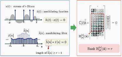
Figure 1: Fundamental duality between sparsity in the image domain and low-rank Hankel matrix in Fourier domain.

In contrast to standard compressed sensing approaches for MRI, the optimization problem in (13) is purely in the measurement domain. After estimating the fully sampled Fourier data, the final reconstruction can be obtained by a simple inverse Fourier transform. This property leads to remarkable flexibility in real-world applications that classical approaches have difficulty exploiting. For example, this formulation has been successfully applied to compressed sensing MRI with state-of-the art performance for single coil imaging [63, 64, 65, 92, 66]. Another flexibility is the recovery of images from multichannel measurements with unknown sensitivities [97, 64]. These schemes rely on the low-rank structure of a structured matrix, obtained by concatenating block Hankel matrices formed from each channel’s data. Similar to L+S decomposition in [85], the L+S model for Hankel structure matrix was also used to remove the $k$-space outliers in MR imaging problems [68]. Such approaches have also been successfully used for super-resolution microscopy [98], image inpainting problems [99], image impulse noise removal [100], etc.

The common thread between sparsity models, low-rank, and structured low-rank models is that they all strive to capture signal redundancies to make up for missing or noisy data.

V Data-Driven and Learning-Based Models

The most recent class of methods constituting the fourth category of image reconstruction schemes exploit data-driven and learning-based models. This section and the next review several of these varied models and methods. The development of efficient algorithms for the often nonconvex learning-based problems is briefly discussed. The pros and cons of various methods, as well as their connections are also discussed.

V-A Partially Data-Adaptive Sparsity-Based Methods

While early reconstruction methods such as in CS MRI used sparsity in known transform domains such as wavelets [15], total variation domain, contourlets [20], etc., later works proposed partially data-adaptive sparsity models by incorporating directional information of patches or block matching, etc., during reconstruction.

A patch-based directional wavelets (PBDW) scheme was proposed for MRI in [101], wherein the regularizer was based on analysis sparsity and was the sum of the $\ell_{1}$ norms of each optimally (adaptively) rearranged and transformed (by fixed 1D Haar wavelets) image patch. The patch rearrangement or permutation involved rearranging pixels parallel to a certain geometric direction, approximating patch rotation. The best permutation for each patch from among a set of pre-defined permutations was pre-computed based on initial reconstructions to minimize the residual between the transformed permuted patch and its thresholded version. An improved reconstruction method was proposed in [102], where the optimal permutations were computed for patches extracted from the subbands in the 2D Wavelet domain (a shift-invariant discrete wavelet transform is used) of the image. A recent work [103] proposed a different effective modification of the PBDW scheme, wherein a unitary matrix is adapted to sparsify the patches grouped with a common (optimal) permutation. In this case, the analysis sparsity penalty during reconstruction used the $\ell_{1}$ norms of patches transformed by the adapted unitary matrices (one per group of patches).

A different fast and effective method (patch-based nonlocal operator or PANO) was proposed in [104], wherein for each patch, a small group of patches most similar to it was pre-estimated (called block matching), and the regularizer during reconstruction penalized the sparsity of the groups of patches in a known transform domain. Another reconstruction scheme based on adaptive clustering of patches was applied to MRI in [105]. All these aforementioned methods are also quite related to the recent transform learning-based methods described in Section V-C, where the sparsifying operators are fully adapted in an optimization framework.

V-B Synthesis Dictionary Learning-Based Approaches for Reconstruction

Among the learning-based approaches that have shown promise for medical image reconstruction, one popular class of methods exploits synthesis dictionary learning.

V-B1 Synthesis Dictionary Model

As briefly discussed in Section III, the synthesis model suggests that a signal can be approximated by a sparse linear combination of atoms or columns of a dictionary, i.e., the signal lives approximately in a subspace spanned by a few dictionary atoms. Because different signals may be approximated with different subsets of dictionary columns, the model is viewed as a union of subspaces model [106].

In imaging, the synthesis model is often applied to image patches (see Fig. 2) or image blocks $\bm{P}_{j}\bm{x}$ as $\bm{P}_{j}\bm{x}\approx\bm{D}\mathbf{z}_{j}$, with $\bm{P}_{j}$ denoting the operator that extracts a vectorized patch (with $n$ pixels) of $\bm{x}$, $\bm{D}\in\mathbb{C}^{n\times K}$ denoting a synthesis dictionary (in general complex-valued), and $\mathbf{z}_{j}\in\mathbb{C}^{K}$ being the sparse representation or code for the patch $\bm{P}_{j}\bm{x}$ with many zeros. While dictionaries based on the discrete cosine transform (DCT), etc., can be used to model image patches, much better representations can be obtained by adapting the dictionaries to data. The learning of synthesis dictionaries has been explored in many works [107, 108, 109] and shown to be promising in inverse problem settings [110, 111, 27].

V-B2 Dictionary Learning for MRI

A dictionary learning-based method for MRI (DL-MRI) was proposed in [27], where the image and the dictionary for its patches are simultaneously estimated from limited measurements. The approach also known as blind compressed sensing (BCS) [30] does not require training data and learns a dictionary that is highly adaptive to the underlying image content. However, the optimization problem is highly nonconvex, and is formulated as follows:

$$\min_{\bm{x},\bm{D},\bm{Z}}\frac{1}{2}\left\|\bm{A}\bm{x}-\bm{y}\right\|_{2}^{2}+\beta\sum_{j=1}^{N}\left\|\bm{P}_{j}\bm{x}-\bm{D}\mathbf{z}_{j}\right\|_{2}^{2}$$

$$\;\;\;\;\text{s.t.}\;\;\begin{Vmatrix}\mathbf{z}_{j}\end{Vmatrix}_{0}\leq s,\;\begin{Vmatrix}\mathbf{d}_{i}\end{Vmatrix}_{2}=1,\;\forall\,i,j.$$ (15)

This corresponds to using a dictionary learning regularizer (weighted by $\beta>0$) of the following form:

$$R(\bm{x})= \min_{\bm{D},\bm{Z}}\sum_{j=1}^{N}\left\|\bm{P}_{j}\bm{x}-\bm{D}\mathbf{z}_{j}\right\|_{2}^{2}$$

$$\;\;\text{s.t.}\;\;\begin{Vmatrix}\mathbf{z}_{j}\end{Vmatrix}_{0}\leq s,\;\begin{Vmatrix}\mathbf{d}_{i}\end{Vmatrix}_{2}=1,\;\forall\,i,j,$$ (16)

where $\bm{Z}$ is a matrix whose columns are the sparse codes $\mathbf{z}_{j}$ that each have at most $s$ non-zeros, and the $\ell_{0}$ “norm” counts the total number of nonzeros in a vector or matrix. The columns $\mathbf{d}_{i}$ of $\bm{D}$ are constrained to have unit norm as otherwise $\mathbf{d}_{i}$ can be scaled arbitrarily along with corresponding inverse scaling of the $i$th row of $\bm{Z}$, and the objective is invariant to this scaling ambiguity.

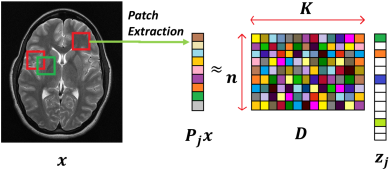
Figure 2: The synthesis dictionary model for image patches: overlapping patches $\bm{P}_{j}\bm{x}$ of the image $\bm{x}$ are assumed approximated by sparse linear combinations of columns of the dictionary $\bm{D}$, i.e., $\bm{P}_{j}\bm{x}\approx\bm{D}\mathbf{z}_{j}$, where $\mathbf{z}_{j}$ has several zeros (denoted with white blocks above).

Problem (15) was optimized in [27] by alternating between solving for the image $\bm{x}$ (image update step) and optimizing the dictionary and sparse coefficients (dictionary learning step). In specific cases such as in single coil Cartesian MRI, the image update step is solved in closed-form using FFTs. However, the dictionary learning step involves a nonconvex and NP-hard optimization problem [112]. Various dictionary learning algorithms exist for this problem and its variants [108, 113, 109] that often alternate between updating the sparse coefficients (sparse coding) and the dictionary. The DL-MRI method for (15) used the K-SVD dictionary learning algorithm [108] and showed significant image quality improvements over previous CS MRI methods that used nonadaptive wavelets and total variation [15]. However, it is slow due to expensive and repeated sparse coding steps, and lacked convergence guarantees. In practice, variable rather than common sparsity levels across patches can be allowed in DL-MRI by using an error threshold based stopping criterion when sparse coding with OMP [114].

V-B3 Other Applications and Variations

Later works applied dictionary learning to dynamic MRI [28, 115, 116], parallel MRI [117], and PET reconstruction [118]. An alternative Bayesian nonparametric dictionary learning approach was used for MRI reconstruction in [119]. Dictionary learning was studied for CT image reconstruction in [25], which compared the BCS approach to pre-learning the dictionary from a dataset and fixing it during reconstruction. The former was found to be more promising when sufficient views (in sparse-view CT) were measured, whereas with very few views (or with very little measured information), pre-learning performed better. Tensor-structured (patch-based) dictionary learning has also been exploited recently for dynamic CT [120] and spectral CT [121] reconstructions.

V-B4 Recent Efficient Dictionary Learning-Based Methods

Recent work proposed efficient dictionary learning-based reconstruction algorithms, dubbed SOUP-DIL image reconstruction algorithms [122] that used the following regularizer:

$$\min_{\bm{D},\bm{Z}}\sum_{j=1}^{N}\begin{Bmatrix}\left\|\bm{P}_{j}\bm{x}-\bm{D}\mathbf{z}_{j}\right\|_{2}^{2}+\lambda^{2}\begin{Vmatrix}\mathbf{z}_{j}\end{Vmatrix}_{0}\end{Bmatrix}\;\;\text{s.t.}\;\;\begin{Vmatrix}\mathbf{d}_{i}\end{Vmatrix}_{2}=1,\;\forall\,i.$$ (17)

Here, the aggregate sparsity penalty $\sum_{j=1}^{N}\left\|\mathbf{z}_{j}\right\|_{0}$ with weight $\lambda^{2}$ automatically enables variable sparsity levels across patches. The dictionary learning step of the SOUP-DIL reconstruction algorithm efficiently optimized (17) using an exact block coordinate descent scheme by decomposing $\bm{D}\bm{Z}$ as a sum of outer products (SOUP) of dictionary columns and rows of $\bm{Z}$, and solving for $\mathbf{d}_{i}$ and then the $i$th row of $\bm{Z}$ (by thresholding) in closed-form, and cycling over all such pairs ($1\leq i\leq K$).

(a)	(b)
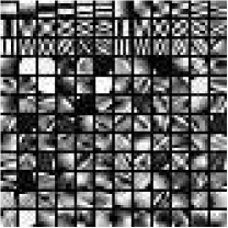
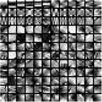
(c)	(d)

Figure 3: Dictionary Learning for MRI (images from [122]): (a) SOUP-DILLO MRI [122] reconstruction (with $\ell_{0}$ penalty) of the water phantom [102]; (b) sampling mask in k-space with 2.5x undersampling; and (c) real and (d) imaginary parts of the dictionary learned during reconstruction, with atoms shown as $6\times 6$ patches.

While the earlier DL-MRI used inexact (greedy) and expensive sparse code updates and lacked convergence analysis, the SOUP-DIL scheme used efficient, exact updates and was proved to converge to the critical points (generalized stationary points) of the underlying problems and improved image quality over several schemes [122]. Fig. 3 shows an example reconstruction with this BCS method along with the learned dictionaries. Another recent work [123] extended the L+S model for dynamic image reconstruction in (7) to a low-rank and adaptive sparse signal model that incorporated a dictionary learning regularizer similar to (17) for the $\bm{x}_{S}$ component.

V-B5 Alternative Convolutional Dictionary Model

One can replace the patch-based dictionary model with a convolutional model as $\bm{x}\approx\sum_{i=1}^{K}\mathbf{d}_{i}\otimes\mathbf{c}_{i}$ that directly represents the image as a sum of (possibly circular) convolutions of dictionary filters $\mathbf{d}_{i}$ and sparse coefficient maps $\mathbf{c}_{i}$ [124, 125]. The convolutional synthesis dictionary model is distinct from the patch-based model. However, its main drawback is the inability to represent very low-frequency content in images, necessitating pre-processing of images to remove very low-frequency content prior to convolutional dictionary learning. The utility of convolutional synthesis dictionary learning for biomedical image reconstruction is an open and interesting area for future research; see [126] for a denoising formulation that could be extended to inverse problems.

V-C Sparsifying Transform Learning-Based Methods

Several recent works have studied the learning of the efficient sparsifying transform model for biomedical image reconstruction [127, 29, 26]. This subsection reviews these advances (see [128] for an MRI focused review).

V-C1 Transform Model

The sparsifying transform model is a generalization [24] of the analysis dictionary model. The latter assumes that applying an operator $\bm{W}$ to a signal $\mathbf{f}$ produces several zeros in the output, i.e., the signal lies in the null space of a subset of rows of the operator. The sparsifying transform model allows for a sparse approximation as $\bm{W}\mathbf{f}=\mathbf{z}+e$, where $\mathbf{z}$ has several zeros and $e$ is a transform domain modeling error. Natural images are well-known to be approximately sparse in transform domains such as the DCT and wavelets, a property that has been exploited for image compression [129], denoising, and inverse problems. A key advantage of the sparsifying transform model compared to the synthesis dictionary model is that the transform domain sparse approximation can be computed exactly and cheaply by thresholding $\bm{W}\mathbf{f}$ [24].

V-C2 Early Efficient Transform Learning-Based Methods

Recent works [127, 29] proposed transform learning based image reconstruction methods that involved computationally cheap, closed-form updates in the iterative algorithms. The following square transform learning [24] regularizer was used for reconstruction in [127]:

$$R(\bm{x})= \min_{\bm{W},\bm{Z}}\sum_{j=1}^{N}\left\|\bm{W}\bm{P}_{j}\bm{x}-\mathbf{z}_{j}\right\|_{2}^{2}+\gamma Q(\bm{W})\;\;\text{s.t.}\;\;\begin{Vmatrix}\bm{Z}\end{Vmatrix}_{0}\leq s,$$ (18)

where $\bm{W}\in\mathbb{C}^{n\times n}$ is a square matrix and the transform learning regularizer $Q(\bm{W})=-\log\left|\det\bm{W}\right|+0.5\left\|\bm{W}\right\|_{F}^{2}$ with weight $\gamma>0$ prevents trivial solutions in learning such as the zero matrix or matrices with repeated rows. Moreover, it also helps control the condition number of the transform [24]. The term $\sum_{j=1}^{N}\left\|\bm{W}\bm{P}_{j}\bm{x}-\mathbf{z}_{j}\right\|_{2}^{2}$ denotes the transform domain modeling error or sparsification error, which is minimized to learn a good sparsifying transform. The constraint in (18) on the $\ell_{0}$ “norm” of the matrix $\bm{Z}$ controls the net or aggregate sparsity of all patches’ sparse coefficients.

The image reconstruction problem with regularizer (18) was solved in [127] using a highly efficient block coordinate descent (BCD) approach that alternates between minimizing with respect to $\bm{Z}$ (transform sparse coding step), $\bm{W}$ (transform update step), and $\bm{x}$ (image update step). Importantly, the transform sparse coding step has a closed-form solution, where the matrix $\bm{B}$, whose columns are $\bm{W}\bm{P}_{j}\bm{x}$, is thresholded to its $s$ largest magnitude elements, with other entries set to zero. When the sparsity constraint is replaced with alternative sparsity promoting functions such as the $\ell_{0}$ sparsity penalty or $\ell_{1}$ penalty, the sparse coding solution is obtained in closed-form by hard or soft thresholding. The transform update step has a simple solution involving the singular value decomposition (SVD) of a small matrix [127] and the image update step involves a least squares problem (e.g., in the case of single coil Cartesian MRI, it is solved in closed-form using FFTs [127]). This efficient BCD scheme was proven to converge in general to the critical points of the nonconvex reconstruction problem [127].

In practice, the sparsity controlling parameter can be varied over algorithm iterations (a continuation strategy), allowing for faster artifact removal initially and then reduced bias over the iterations [29]. The scheme in [127] was shown to be much faster than the previous DL-MRI scheme. Tanc and Eksioglu [130] further combined transform learning with global sparsity regularization in known transform domains for CS MRI.

Square transform learning has also been applied to CT reconstruction [131]. Another recent work used square transform learning for low-dose CT image reconstruction [132] with a shifted-Poisson likelihood penalty for the data-fidelity term in the cost (instead of the conventional weighted least squares penalty), but pre-learned the transform from a dataset and fixed it during reconstruction to save computation.

Other works have explored alternative formulations for transform learning (e.g., overcomplete or tall [133] transforms) that could be potentially used for image reconstruction.

V-C3 Learning Rich Unions of Transforms for Reconstruction

Since, images typically contain a diversity of textures, features, and edge information, recent works [134, 29, 26] learned a union of transforms (a rich model) for image reconstruction. In this setting, a collection of $K$ transforms are learned and the image patches are grouped or clustered into $K$ classes, with each class of (similar) patches best matched to and using a particular transform. The UNITE (UNIon of Transforms lEarning) image reconstruction formulation in [29] uses the following regularizer:

$$R(\bm{x})= \min_{\begin{Bmatrix}\bm{W}_{k},C_{k},\mathbf{z}_{j}\end{Bmatrix}}\sum_{k=1}^{K}\sum_{j\in C_{k}}\begin{Bmatrix}\left\|\bm{W}_{k}\bm{P}_{j}\bm{x}-\mathbf{z}_{j}\right\|_{2}^{2}+\lambda^{2}\begin{Vmatrix}\mathbf{z}_{j}\end{Vmatrix}_{0}\end{Bmatrix}$$

$$\;\;\;\;\;\;\;\;\;\text{s.t.}\;\;\bm{W}_{k}^{H}\bm{W}_{k}=\mathbf{I}\;\forall\,k,\;\begin{Bmatrix}C_{k}\end{Bmatrix}\in G.$$ (19)

Here, $C_{k}$ is a set containing the indices of all patches matched to the transform $\bm{W}_{k}$, and $G$ denotes the set of all partitions of $[1:N]$ into $K$ disjoint subsets, where $N$ is the total number of overlapping patches. Note that when indexed variables are enclosed in braces (in (19) and later equations), we mean the set of all variables over the range of the indices.

The UNITE reconstruction formulation jointly learns a collection of transforms, clusters and sparse codes patches, and reconstructs the image $\bm{x}$ from measurements. An efficient BCD algorithm with convergence guarantees was proposed for optimizing the problem in [29]. The $K$ transforms in (19) are unitary, which simplifies the BCD updates. For MRI, UNITE-MRI achieved improved image quality over the square transform learning-based scheme when reconstructing from undersampled k-space measurements [29].

Figure 4: Cone-beam CT reconstructions (images from [26]) of the XCAT phantom [135] using the FDK, PWLS-EP [136] (with edge-preserving regularizer), and PWLS-ULTRA [26] ($K=15$) methods at dose $I_{0}=5\times 10^{3}$ incident photons per ray, shown along with the ground truth (top left). The central axial, sagittal, and coronal planes of the 3D reconstruction are shown. The learning-based PWLS-ULTRA removes noise and preserve edges much better than the other schemes.

Recent works applied learned unions of transforms to other applications. For example, the union of transforms model was pre-learned (from a dataset) and used in a clustering-based low-dose 3D CT reconstruction scheme [26]. Fig. 4 shows an example of high quality reconstructions obtained with this scheme. While the work used a PWLS-type reconstruction cost, a more recent method [132] replaced the weighted least squares data-fidelity term with the shifted-Poisson likelihood penalty, which further improved image quality and reduced bias in the reconstruction in ultra low-dose settings. Other recent works combined learned union of transforms models with material image models and applied it to image-domain material decomposition in dual-energy CT with high quality results [137, 138].

V-C4 Learning Structured Transform Models

It is often useful to incorporate various structures and invariances in learning to better model natural data, and to prevent learning spurious features in the presence of noise and corruptions. Flipping and rotation invariant sparsifying transform learning was recently proposed and applied to image reconstruction in [139]. The regularization is similar to (19), but using $\bm{W}_{k}=\bm{W}\mathbf{\Phi}_{k}$ with a common parent transform $\bm{W}$ and $\begin{Bmatrix}\mathbf{\Phi}_{k}\end{Bmatrix}$ denoting a set of known flipping and rotation operators that apply to each (row) atom of $\bm{W}$ and approximate flips and rotations by permutations (similar to [101], but which used fixed 1D Haar wavelets as the parent). This enables learning a much more structured but flexible (depending on the number of operators $\mathbf{\Phi}_{k}$) model than in (19), with clustering done more based on similar directional properties. Images with more directional features are better modeled by such learned transforms [139].

V-C5 Learning Complementary Models – Low-rank and Transform Sparsity

A recent work [140] proposed an approach called STROLLR (Sparsifying TRansfOrm Learning and Low-Rank) that combines two complementary regularizers: one exploiting (non-local) self-similarity between regions, and another exploiting transform learning that is based on local patch sparsity. Non-local similarity and block matching models are well-known to have excellent performance in image processing tasks such as image denoising (with BM3D [141]). The STROLLR regularizer has the form $R(\bm{x})=R_{1}(\bm{x})+R_{2}(\bm{x})$, where the low-rank regularizer is as follows:

$$R_{1}(\bm{x})=\min_{\begin{Bmatrix}\mathbf{U}_{j}\end{Bmatrix}}\sum_{j=1}^{N}\begin{Bmatrix}\begin{Vmatrix}{\color[rgb]{0,0,0}\mathcal{M}_{j}(\bm{x})}-\mathbf{U}_{j}\end{Vmatrix}_{F}^{2}+\eta^{2}\,\text{rank}(\mathbf{U}_{j})\end{Bmatrix},$$ (20)

and the transform learning regularizer is

$$R_{2}(\bm{x})= \min_{\bm{W},\begin{Bmatrix}\mathbf{z}_{j}\end{Bmatrix}}\sum_{j=1}^{N}\begin{Bmatrix}\begin{Vmatrix}\bm{W}\mathbf{H}_{j}\bm{x}-\mathbf{z}_{j}\end{Vmatrix}_{2}^{2}+\lambda^{2}\,\begin{Vmatrix}\mathbf{z}_{j}\end{Vmatrix}_{0}\end{Bmatrix}$$

$$\;\;\;\;\;\;\text{s.t.}\;\;\bm{W}^{H}\bm{W}=\mathbf{I}.$$ (21)

Here, the operator $\mathcal{M}_{j}$ is a block matching operator that extracts the $j$th patch $\bm{P}_{j}\bm{x}$ and the $L-1$ patches most similar to it and forms a matrix, whose columns are the $j$th patch and its matched siblings, ordered by degree of match. This matrix is approximated by a low-rank matrix $\mathbf{U}_{j}$ in (20), with $\eta>0$. The vector $\mathbf{H}_{j}\bm{x}$ is a vectorization of the submatrix that is the first $P$ columns of $\mathcal{M}_{j}(\bm{x})$. Thus the regularizer in (21) learns a higher-dimensional transform (e.g., 3D transform for 2D patches), and jointly sparsifies non-local but similar patches.

STROLLR-MRI [140] was shown to achieve better CS MRI image quality over several methods including the supervised (deep) learning based ADMM-Net [142]. Fig. 5 shows example MRI reconstructions and comparisons. Similar to UNITE-MRI, there is an underlying grouping of patches, but STROLLR-MRI exploits block matching and sparsity to implicitly perform grouping.

V-D Online Learning for Reconstruction

Recent works have proposed online learning of sophisticated models for reconstruction particularly of dynamic data from time-series measurements [143, 32, 144]. In this setting, the reconstructions are produced in a time-sequential manner from the incoming measurement sequence, with the models also adapted simultaneously and sequentially over time to track the underlying object’s dynamics and aid reconstruction. Such methods allow greater adaptivity to temporal dynamics and can enable dynamic reconstruction with less latency, memory use, and computation than conventional methods. Potential applications include real-time medical imaging, interventional imaging, etc., or they could be used even for more efficient and (spatially, temporally) adaptive offline reconstruction of large-scale (big) data.

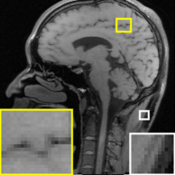
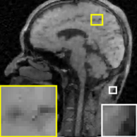
Ground Truth	Sparse MRI
ADMM-Net	STROLLR-MRI

Figure 5: MRI reconstructions (images from [128]) with pseudo-radial sampling and 5x undersampling using Sparse MRI [15] (PSNR = $27.92$ dB), ADMM-Net [142] (PSNR = $30.67$ dB), and STROLLR-MRI [140] (PSNR = $31.98$ dB), along with the original image from [142]. STROLLR-MRI clearly outperforms the nonadaptive Sparse MRI, while ADMM-Net also produces undesirable artifacts.

A recent work efficiently adapted low-rank tensor models in an online manner for dynamic MRI [144]. Online learning for dynamic image reconstruction was shown to be promising in [143, 32], which adapted synthesis dictionaries to spatio-temporal patches. In this setup [32], measurements corresponding to a group (called mini-batch) of frames are processed at a time using a sliding window strategy. The objective function for reconstruction is a weighted time average of instantaneous cost functions, each corresponding to a group of processed frames. An exponential weighting (forgetting) factor for the instantaneous cost functions controls the past memory in the objective. The instantaneous cost functions include both a data-fidelity and a regularizer (corresponding to patches in the group of frames) term. The objective function thus changes over time and is optimized at each time point with respect to the most recent mini-batch of frames and corresponding sparse coefficients (with older frames and coefficients fixed), but the dictionary is itself adapted therein to all the data. Each frame can be reconstructed from multiple overlapping temporal windows and a weighted average of those used as the final estimate.

The online learning algorithms in [32] achieved computational efficiency by using warm start initializations (that improve over time) for variables and frames based on estimates in previous windows, and thus running only a few iterations of optimization for each new window. They stored past information in small (cumulatively updated) matrices for the dictionary update (low memory usage). The methods were significantly more efficient and more effective than batch learning-based techniques for dynamic MRI that iteratively learn and reconstruct from all k-t space measurements. Given the potential of online learning methods to transform dynamic and large-scale imaging, we expect to see growing interest and research in this domain.

V-E Connections between Transform Learning Approaches and Convolutional Network Models

The sparsifying transform models in Section V-C have close connections with convolutional filterbanks. This subsection and the next review some of these connections and implications for reconstruction.

V-E1 Connections to Filterbanks

Transform learning and its application to regularly spaced image patches [145] can be equivalently performed using convolutional operations. For example, applying an atom of the transform to all the overlapping patches of an (2D) image via inner products is equivalent to convolving the image with a transform filter that is the (2D) flipped version of the atom. Thus, sparse coding in the transform model can be viewed as convolving the image with a set of transform filters (obtained from the transform atoms) and thresholding the resulting filter coefficient maps, and transform learning can be viewed as equivalently learning convolutional sparsifying filters [146, 147]. When using only a regularly spaced subset of patches, the above interpretation of transform sparse coding modifies to convolving the image with the transform filters, downsampling the results, and then thresholding [145]. Transform models based on clustering [29] add non-trivial complexities to this process.

Applying the matrix $\bm{W}^{H}$ to the sparse codes of all overlapping patches and spatially aggregating the results, an operation used in iterative transform-based reconstruction algorithms [29], is equivalent to filtering the thresholded filter coefficient maps with corresponding matched filters (complex conjugate of transform atoms) and summing the results over the channels. These equivalences between patch-based and convolutional operations for the transform model contrast with the case for the synthesis dictionary model in Section V-B, where the patch-based and convolutional versions of the model are not equivalent in general. When a disparate set of (e.g., randomly chosen) image patches or operations such as block matching [140], etc., are used with the transform model, the underlying operations do not correspond to convolutions (thus, the transform learning frameworks can be viewed as more general). Typically the convolutional implementation of transforms is more computationally efficient than the patch-based version for large filter sizes [145].

Recent works have exploited the filterbank interpretation of the transform model [145, 148, 149]. For example, [150] learned filterbanks for MRI reconstruction. In  [145], the authors studied alternative properties and regularizers for transform learning.

V-E2 Multi-layer Transform Learning

A recent work [149] proposed learning multi-layer extensions of the transform model (dubbed deep residual transforms (DeepResT)) that mimic convolutional neural networks (CNNs) by incorporating components such as filtering, nonlinearities, pooling, and stacking; however, the learning was done using unsupervised model-based transform learning-type cost functions.

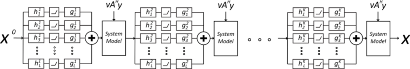
Figure 6: The reconstruction model (see [148]) derived from the image update step of the square transform learning-based image reconstruction algorithm in [29]. The model here has $K$ layers corresponding to $K$ iterations. Each layer first has a decorruption step that computes the second term in (22) using filtering and thresholding operations, assuming a transform model with $L$ filters. This is followed by a system model block that adds the fixed bias term $\nu\bm{A}^{H}\bm{y}$ to the output of the decorruption step and performs a least-squares type image update (e.g., using CG) to enforce the imaging forward model.

In the conventional transform model, the image is passed through a set of transform filters and thresholded (the non-linearity) to generate the sparse coefficient maps. In the DeepResT model, the residual (difference) between the filter outputs and their sparse versions is computed and these residual maps for different filters are stacked together to form a residual volume that is jointly sparsified in the next layer. To prevent dimensionality explosion, each filtering of the residual volume in the second and subsequent layers produces a 2D output (for a 2D initial image). The multi-layer model thus consists of successive joint sparsification of residual maps several times (cf. Fig. 1 in [149] and Fig. 9 in [128]). The filters and sparse maps in all layers of the (encoder) network are jointly and efficiently learned in [149] from images to provide the smallest sparsification residuals in the final (output) layer, a transform learning-type cost. The learned model and multi-layer sparse coefficient maps can then be backpropagated in a linear fashion (decoder) to generate image approximations. The DeepResT model also downsampled (pooled) the residual maps (along the filter channel dimension) in each encoder layer before further filtering them, providing robustness to noise and data corruptions. The learned models were shown [149] to provide promising performance for denoising images when learning directly from noisy data, and moreover learning stacked multi-layer encoder-decoder modules was shown to improve performance, especially at high noise levels. Application of such deep transform models to medical image reconstruction is an ongoing area [151] of potent research.

V-F Physics-Driven Deep Training of Transform-Based Reconstruction Models

There has been growing recent interest in supervised learning approaches for image reconstruction [33]. These methods learn the parameters of reconstruction algorithms from training datasets (typically consisting of pairs of ground truth images and initial reconstructions from measurements) to minimize the error in reconstructing the training images from their typically limited or corrupted measurements. For example, the reconstruction model can be a deep CNN (typically consisting of encoder and decoder parts) that can be trained (as a denoiser) to produce a reconstruction from an initial corrupted version [34]. Section VI discusses such approaches in more detail. These methods can often require large training sets to learn billions of parameters (e.g., filters, etc.). Moreover, learned CNNs (deep learning) may not typically or rigorously incorporate the imaging measurement model or the information about the Physics of the imaging process, which are a key part of solving inverse problems. Hence, there has been recent interest in learning the parameters of iterative algorithms that solve regularized inverse problems [142, 35] (cf. Section VI for more such methods). These methods can also typically have fewer free parameters to train.

Recent works have interpreted early transform-based BCS algorithms as deep physics-driven convolutional networks learned on-the-fly, i.e., in a blind manner, from measurements [35, 148]. For example, the image update step in the square transform BCS (that learns a unitary transform) algorithm in [29] involves a least squares-type optimization with the following normal equation:

$$\bm{G}\bm{x}^{k}=\nu\bm{A}^{H}\bm{y}+\sum_{j=1}^{N}\bm{P}_{j}^{T}\bm{D}^{k}\bm{H}_{\lambda}(\bm{W}^{k}\bm{P}_{j}\bm{x}^{k-1}),$$ (22)

where $\nu=1/\beta$ (for $\beta$ in Section V-B or V-C) and $k$ denotes the iteration number in the block coordinate descent reconstruction algorithm. Matrix $\bm{D}^{k}\triangleq\begin{pmatrix}\bm{W}^{k}\end{pmatrix}^{H}$ is a (matched) synthesis operator, and $\bm{G}\triangleq\sum_{j=1}^{N}\bm{P}_{j}^{T}\bm{P}_{j}+\nu\bm{A}^{H}\bm{A}$ is a fixed matrix. The hard-thresholding in (22) corresponds to the solution of the sparse coding step of the BCD algorithm [29].

Fig. 6 shows an unrolling of $K$ iterations (layers) of (22), with fresh filters in each iteration. Each layer has a system model block that solves (22) (e.g., with FFTs or CG), whose inputs are the two terms on the right hand side of (22): the first term is a fixed bias term; and the second term (denotes a decorruption step) is computed via convolutions by first applying the transform filters (denoted by $h_{l}^{k}$, $1\leq l\leq L$ in Fig. 6) followed by thresholding (the non-linearity) and then matched synthesis filters (denoted by $g_{l}^{k}$, $1\leq l\leq L$), and summing the outputs over the filters. This is clear from writing the second term in (22) as $\sum_{l=1}^{L}\sum_{j=1}^{N}\bm{P}_{j}^{T}\mathbf{d}_{l}^{k}\bm{H}_{\lambda}(\mathbf{r}_{l}^{k^{T}}\bm{P}_{j}\bm{x}^{k-1})$, with $\mathbf{d}_{l}$ and $\mathbf{r}_{l}$ denoting the $l$th columns of $\bm{D}$ and $\mathbf{R}=\bm{W}^{T}$, respectively. Each of the $L$ terms forming the outer summation here corresponds to the output of an arm (of transform filtering, thresholding, and synthesis filtering) in the decorruption module of Fig. 6. Since the BCS scheme in [29] does not use training data, but rather learns the transform filters as part of the iterative BCD algorithm (hence, the transform could change from iteration to iteration or layer to layer), it can be interpreted as learning the model in Fig. 6 in an on-the-fly sense from measurements.

Recent works [35, 148] learned the filters in this multi-layer model (a block coordinate descent or BCD Net [152]) with soft-thresholding ($\ell_{1}$ norm-based) nonlinearities and trainable thresholds using a greedy scheme to minimize the error in reconstructing a training set from limited measurements. These and similar approaches (including the transform-based ADMM-Net [142]) involving unrolling of typical image reconstruction algorithms are physics-driven deep training methods due to the systematic inclusion of the imaging forward model in the convolutional network. Once learned, the reconstruction model can be efficiently applied to test data using convolutions, thresholding, and least squares-type updates. While [35, 148] did not enforce the corresponding synthesis and transform filters (in each arm of the decorruption module) to be matched in each layer, recent work [152] learned matched filters, improving image quality. The learning of such physics-driven networks is an active area of research, with interesting possibilities for new innovation in the convolutional models in the architecture motivated by more recent transform and dictionary learning based (or other) reconstruction methods. In such methods, the thresholding operation is the key to exploiting sparsity.

VI Deep Learning Methods

One of the most important recent developments in the field of image reconstruction is the introduction of deep learning approaches [38]. Motivated by the tremendous success of deep learning for image classification[153, 154], image segmentation[155], denoising [156], etc, many groups have recently successfully applied deep learning approaches to various image reconstruction problems such as in X-ray CT [157, 158, 159, 160, 161, 162, 163], MRI [164, 165, 166, 167, 162, 33, 168], PET [169, 170] ultrasound [171, 172], and optics [173, 174, 175]. As of mid 2019, two commercial CT vendors received FDA approval for deep learning image reconstruction [176] [177].

The sharp increase in deep learning approaches for image reconstruction problems may be due to the “perfect storm” resulting from a combination of multiple attributes in perfect timing: availability of large public data, well-established GPU infrastructure in the image reconstruction community, easy-to-access deep learning toolboxes, industrial push, and open publications using arXiv, etc.

For example, one important public data set that has significantly contributed to this wave is the 2016 American Association of Physicists in Medicine (AAPM) Low-Dose X-ray CT Grand Challenge data set [178]. The training data sets consist of normal-dose and quarter-dose abdominal CT data from ten patients. Another emerging important data set is the fast MRI data set by NYU Langone Health and Facebook [179]. The dataset comprises raw k-space data from more than 1,500 fully sampled knee MRIs and DICOM images from 10,000 clinical knee MRIs obtained at 3 Tesla or 1.5 Tesla.

In addition, GPU methods have been extensively implemented to accelerate iterative methods in the field of image reconstruction. As a result, open deep learning toolboxes such as Tensorflow, pyTorch, MatConvNet, etc., based on GPU programming, are easily accessible to researchers in the field of image reconstruction. Moreover, the industry has been engaging in a big push in this development from the early phase, since deep learning based image reconstruction methods are well-suited to their business models. This is because the training can be done by the vendors with large databases and the users could enjoy high quality reconstruction results at near real-time reconstruction speed.

Given the relatively long publication cycle for regular journals in the field of image reconstruction, most new developments are found in arXiv preprints, well before they are formally accepted by the journals. This new trend of open publication facilitates the significant progress in this area within a short time period. The following subsection reviews the recent developments based on the peer-reviewed publications and arXiv preprints.

VI-A Categories of the existing approaches

This section starts with reviews of various network architectures and design principles for image reconstruction problems. Fig. 7 illustrates typical architectures at a high level, which are commonly used in the literature. However, this field is rapidly growing, so a complete review of the design principles is beyond the scope of the paper.

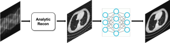
(a) Image-domain Learning

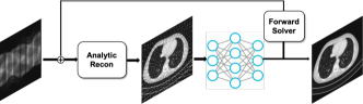
(b) Hybrid-domain Learning

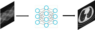
(c) AUTOMAP

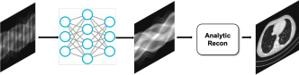
(d) Sensor-domain Learning

Figure 7: Various realizations of deep learning for image reconstruction.

VI-A1 Image-domain learning

In image domain approaches [165, 180, 157, 181, 162, 167, 163, 158, 161], artifact-corrupted images are first generated from the measurement data using some analytic methods (e.g., FBP, Fourier transform, etc.), from which neural networks are trained to learn the artifacts (see Fig. 7(a)). For example, the low-dose and sparse CT neural networks [157, 181, 162, 163, 158, 161] belong to this class, where the noise corrupted images are first generated from the noisy or sparse view sinogram data using FBP, after which the artifacts are learned by comparing with the noiseless label images. In MR applications, the early U-Net architectures for compressed sensing MRI [182, 167] were also designed to remove the aliasing artifacts after obtaining the Fourier inversion image from the downsampled k-space data.

In particular, FBPConvNet [162] showed that image domain networks can be derived by unrolling sparse recovery for one specific class of inverse problems: those where the normal operator associated with the forward model is a convolution. For this class of inverse problems, a CNN then emerges. This class of normal operators includes MRI, parallel-beam X-ray CT, and diffraction tomography (DT).

A current trend in image domain learning is to use more sophisticated loss functions to overcome the observed smoothing artifacts. For example, in [183], the authors used the perceptual loss and Wasserstein distance loss to improve the resolution.

VI-A2 Hybrid-domain learning

In this class of approaches [165, 142, 164, 142, 33, 184, 160, 166, 159, 185, 186, 187, 188, 189], the data consistency term is imposed in the neural network training and inference to improve the performance as shown in Fig. 7(b). The physics-driven deep training methods in Section V-F included the full data-fidelity based image update in each layer.

The Learned ISTA (LISTA) [190] is one of the earliest unfolding approaches that uses a time unfolded version of the iterative soft-threshodling (ISTA) [191]. Specifically, the weight matrices and sparsifying soft-thresholding operator are learned from the data (as also done in later works discussed in Section V-F).

The variational neural network for compressed sensing MRI [165] derived an unrolled neural network that uses a data consistency term for each layer. Specifically, the variational network is based on unfolding the following optimization problem:

$$\min_{\bm{x}}\frac{\lambda}{2}\|\bm{y}-\bm{A}\bm{x}\|^{2}+\mathcal{R}(\bm{x}),$$ (23)

where the regularization term $\mathcal{R}(\bm{x})$ is represented as a sum of multichannel operations:

$$\mathcal{R}(\bm{x})=\sum_{i=1}^{M}\langle\Phi_{i}(\bm{K}_{i}\bm{x}),\mathbf{1}\rangle,$$ (24)

where $\bm{K}_{i}$ denotes the $i$th linear operator represented by the $i$th channel convolution (like the transform filters in Section V), and $\Phi_{i}$ denotes the associated activation function. In a variational network [165], the convolution-based linear operator $\bm{K}_{i}$, the gradient of the activation function $\Phi_{i}^{\prime}$, and the regularization parameter $\lambda^{k}$ are learned for each unfolded Landweber iteration steps. Related approaches have been taken in dynamic cardiac MRI [33].

In ADMM-Net [142], the unrolled steps of the alternating direction method of multipliers (ADMM) based reconstruction algorithm are mapped to each layer of a deep neural network. Recently, the primal-dual algorithm was extended to obtain a CNN-based learned primal-dual approach [160]. In this approach, two neural networks are learned for the primal step and dual step. The projected gradient method has also been extended to a neural network approach [184].

Another class of popular hybrid domain approaches is based on the CNN penalty and plug-and-play model. Specifically, in CNN penalty approaches [164], a neural network is used as a prior model within an MBIR framework. Rather than using a CNN penalty explicitly, in the plug-and-play approach [189, 188], the denoising step of an iteration like ADMM is replaced with a neural network denoiser. Similarly, the deep image prior approach [192] formulates the image reconstruction problem as

$$\min_{{\bm{\theta}}} \frac{\lambda}{2}\|\bm{y}-\bm{A}\bm{z}({\bm{\theta}})\|^{2}+\mathcal{R}(\bm{z}({\bm{\theta}}))$$ (25)

subject to $$\bm{z}({\bm{\theta}})=\bm{G}_{{\bm{\theta}}}(\mathbf{v}),$$ (26)

where $\bm{G}_{\bm{\theta}}$ is a deep neural network parameterized by ${\bm{\theta}}$. The dimension of the parameter ${\bm{\theta}}$ is usually determined by the neural network architecture. In the original deep prior model [192], the input ($\mathbf{v}$) for the neural network was a noise vector. Instead, in its recent application to PET image reconstruction [170], simultaneously acquired MRI data was used as the input to the neural network for PET reconstruction using deep image prior.

VI-A3 AUTOMAP

The Automated Transform by Manifold Approximation (AUTOMAP) [168] (see Fig. 7(c)) approach learns a direct mapping from the measurement domain to image domain using a neural network. This approach requires a fully connected layer followed by convolution layers, leading to high memory requirements for storing that fully connected layer, currently limiting AUTOMAP applications to small size reconstruction problems in MRI.

VI-A4 Sensor-domain learning

Sensor-domain learning approaches try to learn the sensor domain interpolation and denoising using a neural network as shown in Fig. 7(d). For low-dose CT, [193] designed a neural network in the projection domain, yet the neural network is trained in an end-to-end manner from the sinogram to the image domain. Accordingly, the final output of the neural network is a data-driven ramp filter designed by minimizing the image domain loss. Metal artifact correction in CT is another opportunity for sensor-domain learning [194, 195]. For low-dose CT and sparse view CT, direct sinogram domain processing using deep neural network was also proposed [196, 197]. In k-space deep learning for accelerated MRI [198, 199, 200], neural networks were designed to learn k-space interpolation kernels in an end-to-end manner from k-space to the image domain using an image domain loss.

VI-A5 Some variations

In [157], the neural networks were designed to learn the relationship between contourlet transform coefficients of the low-dose input and high dose label data. Later, this problem is formally extended to wavelet domain residual network (WavResNet) to improve the performance [159] (see Fig. 8 for an example). Here, the choice of appropriate transform domain facilitating efficient learning is important and usually based on domain expertise. For example, in a recent deep neural network architecture for interior tomography problems, [201] observed that the neural network is more robust with respect to different ROI sizes, detector pitch, short scan and sparse view artifacts, if the neural network is designed in the differentiated backprojection (DBP) domain. The DBP is well-known in the CT community for its robustness to short scan artifact, interior tomography, etc, which clearly shows the importance of domain expertise in designing neural networks.

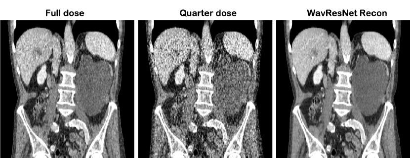
Figure 8: Left to right: full-dose FBP reconstruction, quarter-dose FBP reconstruction, and WavResNet denoising results [159] applied to 25% dose FBP images. The detailed textures, vessel structure, and cancer lesions are clearly seen in the denoised results.

VI-B Semi-supervised and Unsupervised Learning

Most deep learning approaches for image reconstruction have been based on the supervised learning framework. For example, in the low-dose CT reconstruction problems, the neural network is trained to learn the mapping between the noisy image and the noiseless (or high dose) label images. Similar approaches are taken in accelerated MRI, where the relationship between highly accelerated and artifact corrupted input and the fully sampled label data are learned using training data.

Unfortunately, in many imaging scenarios the noiseless label images are difficult to obtain or even impossible to acquire. For example, in low-dose CT problems, an institutional reviewer board (IRB) rarely approves experiments that would require two exposures at low and high dose levels due to the potential risks to patients. This is why in the AAPM X-ray CT Low-Dose Grand Challenge, the matched low-dose images were generated by adding synthetic noise to the full dose sinogram data. Even in accelerated MRI, high-resolution fully sampled k-space data is very difficult to acquire due to the long scan time, and impossible to collect for dynamic MRI data sets that are all inherently under-sampled. Therefore, neural network training without reference or with small reference pairs are very important in the field of image reconstruction.

One of the earliest works in this regard was a low-dose CT denoising network [161]. Instead of using matched high-dose data, the authors employ the GAN loss to match the probability distribution. One of the limitations of this work is that the network is very sensitive and, without careful training, spurious artifacts are often generated due to the generative nature of GAN. To address this problem, a cycleGAN architecture employed cyclic loss and identity loss for multiphase cardiac CT problems [202]. Thanks to the two loss functions, the authors demonstrated that no spurious artifact appeared in their results even without reference data.

Besides, several of the learning approaches in Section V also do not require reference data (or can use limited reference data) to provide high quality reconstructions.

VI-C Interpretation of Deep Models

One of the major hurdles of the deep learning approaches for image reconstruction is the black-box nature of neural networks. This is especially problematic for medical imaging applications, since many clinicians are concerned about whether the performance improvement is real or cosmetic.

The modern reconstruction techniques, such as compressed sensing, can be considered as representation learning methods that aim at finding the optimal parsimonious representation under the data fidelity term. Unfortunately, the classical approaches usually require computationally expensive optimization methods to find the optimal representation. One of the important take-home messages of this section is to show that deep learning approaches are indeed another form of representation learning approaches, which have advantages compared to the classical approaches. In the following, we start to revisit the classical approaches in this aspect.

VI-C1 Image Reconstruction via Representation Learning

One can formulate image reconstruction problems as

$$\min_{\bm{x}\in{\bm{\mathcal{X}}}} \|\bm{y}-\bm{A}\bm{x}\|^{2},$$ (27)

where ${\bm{\mathcal{X}}}$ denotes the low dimensional manifold where the unknown $\bm{x}$ lives. For example, ${\bm{\mathcal{X}}}$ can be represented by

$${\bm{\mathcal{X}}}=\left\{\bm{x}~{}|~{}\bm{x}=\sum_{i\in I}\langle{\bm{b}}_{i},\bm{x}\rangle\tilde{\bm{b}}_{i},\right\}$$ (28)

where $I\subseteq\mathbb{N}$ is an index set (for example, in compressed sensing, $I$ is a sparse index set such that the signal can be represented as a sparse combination of basis elements.) Here, a family of functions $\{{\bm{b}}_{i}\}_{i\in\mathbb{N}}$ is usually selected as a frame that satisfies the following equality [203]:

$$A\|\bm{x}\|^{2}\leq\sum_{i\in\mathbb{N}}|\langle{\bm{b}}_{i},\bm{x}\rangle|^{2}\leq B\|\bm{x}\|^{2},\quad\forall\bm{x}\in H,$$ (29)

where $A,B>0$ are called the frame bounds, and $H$ denotes the specific Hilbert space. If $A=B$, then the frame is called a tight frame. In (28), another family of functions $\{\tilde{\bm{b}}_{i}\}_{i\in\mathbb{N}}$ form the dual frame satisfying the equality:

$$\sum_{i\in\mathbb{N}}\langle{\bm{b}}_{i},\tilde{\bm{b}}_{i}\rangle=1.$$

If the frame basis is chosen in a multiresolution manner, it is called framelet. In compressed sensing, the frames are usually chosen from wavelet transforms, learned dictionaries, or other redundant bases, where the sparse combination of a subset of the frame can represent the unknown signals with high accuracy.

Even for recent approaches such as low-rank Hankel structured matrix completion approaches, the same frame interpretation exists. Specifically, for a given low-rank Hankel matrix $\bm{\mathbb{H}}_{[d]}^{[n]}(\bm{x})$, let ${\bm{\Phi}}=[{\bm{\phi}}_{1},\cdots,{\bm{\phi}}_{n}]\in{\mathbb{R}}^{n\times n}$ and ${\bm{\Psi}}=[{\bm{\psi}}_{1},\cdots,{\bm{\psi}}_{d}]\in{\mathbb{R}}^{d\times d}$ denote the arbitrary basis matrices that are multiplied to the left and right of the Hankel matrix, respectively. Yin et al. derived the following signal expansion, which they called the convolution framelet expansion [204]:

$$\bm{x} = \frac{1}{d}\sum_{i=1}^{n}\sum_{j=1}^{d}\langle\bm{x},{\bm{\phi}}_{i}\circledast{\bm{\psi}}_{j}\rangle{\bm{\phi}}_{i}\circledast{\bm{\psi}}_{j},$$ (30)

implying that $\{{\bm{\phi}}_{i}\circledast{\bm{\psi}}_{j}\}_{i,j=1}^{n,d}$ is a tight frame.

The observations imply that an efficient and concise signal representation is important for the success of modern image reconstruction approaches, and specific algorithms may differ in their choice of the frame basis and specific method to identify the sparse subset that concisely represents the signal.

In this perspective, the classical approaches such as CS, structured low-rank Hankel matrix approaches, etc. have two fundamental limitations. First, the choice of the underlying frame (and its dual) is based on top-down design principles. For example, most of wavelet theory has been developed around the edge-adaptive basis representations such as curvelet [205], contourlet [206], etc., whose design principle is based on top-down mathematical modeling. Moreover, the search for the sparse index set $I$ for the case of compressed sensing is usually done using a computationally expensive optimization framework. The following section shows that these limitations of classical representation learning approaches can be largely overcome by deep learning approaches.

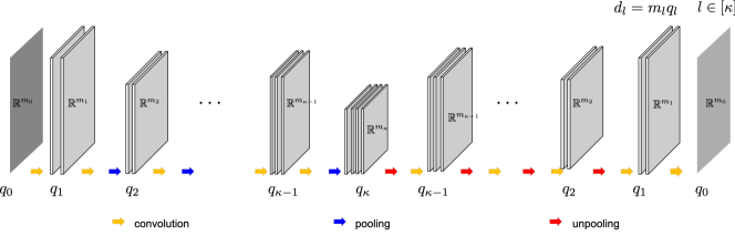
Figure 9: An example of encoder-decoder CNN. The encoder is composed of the first $\kappa$ layers, while the latter $\kappa$ layers form a decoder network.

VI-C2 Deep Neural Networks as Combinatorial Representation Learning

The recent theory of deep convolutional framelets claims that a deep neural network can be interpreted as a framelet representation, whose frame basis is learned from the training data [207]. Moreover, a recent follow-up study [208] showed how this frame representation can be automatically adapted to various input signals in a real-time manner.

To understand these findings, consider the symmetric encoder-decoder CNN in Fig. 9, which has been used for image reconstruction problems [162, 163]. Specifically, the encoder network maps a given input signal $\bm{x}\in{\bm{\mathcal{X}}}\subset{\mathbb{R}}^{d_{0}}$ to a feature space $\bm{z}\in{\bm{\mathcal{Z}}}\subset{\mathbb{R}}^{d_{\kappa}}$, whereas the decoder takes this feature map as an input, processes it, and produces an output $\bm{y}\in{\bm{\mathcal{Y}}}\subset{\mathbb{R}}^{d_{0}}$. At the $l$th layer, $m_{l}$, $q_{l}$, and $d_{l}:=m_{l}q_{l}$ denote the dimension of the signal, the number of filter channels, and the total feature vector dimension, respectively. We consider a symmetric configuration, where both the encoder and decoder have the same number of layers, say $\kappa$; and the encoder layer ${{\mathcal{E}}}^{l}$ and the decoder layer ${{\mathcal{D}}}^{l}$ are symmetric.

$${{\mathcal{E}}}^{l}:{\mathbb{R}}^{d_{l-1}} \mapsto {\mathbb{R}}^{d_{l}},$$

$${{\mathcal{D}}}^{l}:{\mathbb{R}}^{d_{l}} \mapsto {\mathbb{R}}^{d_{l-1}}$$

The $j$th channel output from the the $l$th layer encoder can be represented by a multi-channel convolution operation [208]:

$$\bm{x}_{j}^{l}=\sigma\left({\bm{\Phi}}^{l\top}\sum_{k=1}^{q_{l-1}}\left(\bm{x}_{k}^{l-1}\circledast\overline{\bm{\psi}}_{j,k}^{l}\right)\right),$$ (31)

where $\bm{x}_{k}^{l-1}$ denotes the $k$th input channel signal, $\overline{\bm{\psi}}_{j,k}^{l}\in{\mathbb{R}}^{r}$ denotes the $r$-tap convolutional kernel that is convolved with the $k$th input channel to contribute to the $j$th channel output, and ${\bm{\Phi}}^{l\top}$ is the pooling operator. Here, $\overline{\bm{v}}$ is the flipped version of the vector $\bm{v}$ such that $\overline{v}[n]=v[-n]$ with the periodic boundary condition, and $\circledast$ is the circular convolution. (Using periodic boundary conditions simplifies the mathematical treatments.) Similarly, the $j$th channel decoder layer convolution output is given by [208]

$$\tilde{}\bm{x}_{j}^{l-1}=\sigma\left(\sum_{k=1}^{q_{l}}\left(\tilde{\bm{\Phi}}^{l}\tilde{}\bm{x}^{l}_{k}\circledast{\tilde{\bm{\psi}}_{j,k}^{l}}\right)\right),$$ (32)

where $\tilde{\bm{\Phi}}^{l}$ denotes the unpooling operator, $\tilde{}\bm{x}_{k}^{l}$ denotes the $k$th input channel signal for the decoder, and $\tilde{\bm{\psi}}_{j,k}^{l}\in{\mathbb{R}}^{r}$ denotes the $r$-tap convolutional kernel that is convolved with the $k$th input channel to contribute to the $j$th channel output.

By concatenating the multi-channel signal in column direction as

$$\bm{x}^{l}:=\begin{bmatrix}\bm{x}^{l\top}_{1}&\cdots&\bm{x}^{l\top}_{q_{l}}\end{bmatrix}^{\top},$$

the encoder and decoder convolution in (31) and (32) can be represented using matrix notation:

$$\bm{x}^{l}=\sigma({\bm{E}}^{l\top}\bm{x}^{l-1}), \tilde{}\bm{x}^{l-1}=\sigma({\bm{D}}^{l}\tilde{}\bm{x}^{l})$$ (33)

where $\sigma(\cdot)$ denotes the element-wise rectified linear unit (ReLU) and

$$\bm{E}^{l}=\begin{bmatrix}{\bm{\Phi}}^{l}\circledast{\bm{\psi}}^{l}_{1,1}&\cdots&{\bm{\Phi}}^{l}\circledast{\bm{\psi}}^{l}_{q_{l},1}\\ \vdots&\ddots&\vdots\\ {\bm{\Phi}}^{l}\circledast{\bm{\psi}}^{l}_{1,q_{l-1}}&\cdots&{\bm{\Phi}}^{l}\circledast{\bm{\psi}}^{l}_{q_{l},q_{l-1}}\end{bmatrix}$$ (34)

$${\bm{D}}^{l}=\begin{bmatrix}\tilde{\bm{\Phi}}^{l}\circledast\tilde{\bm{\psi}}^{l}_{1,1}&\cdots&\tilde{\bm{\Phi}}^{l}\circledast\tilde{\bm{\psi}}^{l}_{1,q_{l}}\\ \vdots&\ddots&\vdots\\ \tilde{\bm{\Phi}}^{l}\circledast\tilde{\bm{\psi}}^{l}_{q_{l-1},1}&\cdots&\tilde{\bm{\Phi}}^{l}\circledast\tilde{\bm{\psi}}^{l}_{q_{l-1},q_{l}}\end{bmatrix}$$ (35)

and

$${\bm{\Phi}}^{l}=\begin{bmatrix}{\bm{\phi}}^{l}_{1}&\cdots&{\bm{\phi}}^{l}_{m_{l}}\end{bmatrix},$$

$$\begin{bmatrix}{\bm{\Phi}}^{l}\circledast{\bm{\psi}}_{i,j}^{l}\end{bmatrix}:=\begin{bmatrix}{\bm{\phi}}^{l}_{1}\circledast{\bm{\psi}}_{i,j}^{l}&\cdots&{\bm{\phi}}^{l}_{m_{l}}\circledast{\bm{\psi}}_{i,j}^{l}\end{bmatrix}.$$

Then, one of the most important observations is that the output of the encoder-decoder CNN can be represented as follows [208]:

$$\bm{y} = \sum_{i}\langle{\bm{b}}_{i}(\bm{x}),\bm{x}\rangle\tilde{\bm{b}}_{i}(\bm{x}),$$ (36)

where ${\bm{b}}_{i}(\bm{x})$ and $\tilde{\bm{b}}_{i}(\bm{x})$ denote the $i$th columns of the following frame basis and its dual:

$$\bm{B}(\bm{x}) = {\bm{E}}^{1}{\bm{\Sigma}}^{1}(\bm{x}){\bm{E}}^{2}\cdots{\bm{\Sigma}}^{\kappa-1}(\bm{x}){\bm{E}}^{\kappa},~{}\quad$$ (37)

$$\tilde{}\bm{B}(\bm{x}) = {\bm{D}}^{1}\tilde{\bm{\Sigma}}^{1}(\bm{x}){\bm{D}}^{2}\cdots\tilde{\bm{\Sigma}}^{\kappa-1}(\bm{x}){\bm{D}}^{\kappa},$$ (38)

and ${\bm{\Sigma}}^{l}(\bm{x})$ and $\tilde{\bm{\Sigma}}^{l}(\bm{x})$ denote diagonal matrices with 0 and 1 values that are determined by the ReLU output in the previous convolution steps. Similar basis representation holds for the encoder-decoder CNNs with skipped connection. For more details, see [208].

In the absence of ReLU nonlinearities, the authors in [207, 208] showed that, assuming that the pooling and unpooling operators and the filter matrices satisfy appropriate frame conditions for each $l$, the representation (36) is indeed a frame representation of $\bm{x}$ as in (28), ensuring perfect signal reconstruction. However, in neural networks the input and output should differ, so the perfect reconstruction condition is not of practical interest. Furthermore, the signal representation in (36) should generalize well for various inputs rather than for specific inputs at the training phase.

Indeed, [208] shows that the explicit dependence on the input $\bm{x}$ in (37) and (38) due to the ReLU nonlinearity solves the riddle, and CNN generalizability comes from the combinatorial nature of the expansion in (36) due to the ReLU.

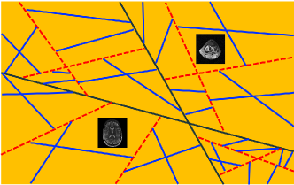
Figure 10: A high level illustration of input space partitioning for the three layer neural network with two filter channels for each layer. Input images at each partition share the same linear representation, but not across different partitions.

Specifically, since the nonlinearity is applied after the convolution operation, the on-and-off activation pattern of each ReLU determines a binary partition of the feature space at each layer across the hyperplane that is determined by the convolution. Accordingly, in deep neural networks, the input space ${\bm{\mathcal{X}}}$ is partitioned into multiple non-overlapping regions as shown in Fig. 10 so that input images for each region share the same linear representation, but not accross the partition. This implies that two different input images in Fig. 10 are automatically switched to two distinct linear representations that are different from each other.

This input adaptivity poses an important computational advantage over the classical representation learning approaches that rely on computationally expensive optimization techniques. Moreover, the representations are entirely dependent on the filter sets that are learned from the training data set, which is different from the classical representation learning approaches that are designed by mathematical principles. Furthermore, the number of input space partitions and the associated distinct linear representations increases exponentially with the network depth, width, and the skipped connection thanks to the combinatorial nature of ReLU nonlinearities [208]. This exponentially large expressivity of the neural network is another important advantage, which may, with the combination of the aforementioned adaptivity, may explain the origin of the success of deep neural networks for image reconstruction.

VII Open Questions and Future Directions

There are various challenges, open questions, and directions for image reconstruction that require further research. This section discusses some possible directions.

As background for this section, it is useful to recall the general topics of past (and ongoing) image reconstruction research, many of which are encapsulated in (1). The likelihood $p(\bm{y};\bm{x})$ depends on both accurate physical modeling of the imaging system, and accurate statistical modeling of the measurements. Numerous papers have focused on improving image quality by more accurate models for imaging physics or statistics. Often more accurate models require more computation so there is an engineering challenge to make accurate models computationally tractable for routine use. Some imaging systems, like MRI, have quite flexible sampling patterns and the chosen sampling pattern is also embedded in the likelihood. The design of effective sampling patterns is an active research area in MRI. The prior $p(\bm{x})$, or the regularizer $R(\bm{x})$ depends on models for the signal $\bm{x}$. Numerous papers have focused on this aspect, and many of the open problems listed below also relate to signal models. The “$\arg\min$” in (1) requires an optimization algorithm, and numerous papers have proposed algorithms (often with various properties such as rapid theoretical or empirical convergence, or whose computations scale well to large-scale settings, etc.) for specific image reconstruction problems. This will continue to be an active research area because new signal models lead to new optimization problems. Furthermore, many deep-learning methods for image reconstruction are based on “unrolling” some optimization algorithm.

After performing optimization to get an image $\hat{\bm{x}}$, the research continues because the field needs task-based metrics to quantify the quality of $\hat{\bm{x}}$. Objective assessment of image quality is an ongoing research area [209] that should have more influence on image reconstruction research in the future because traditional measures like mean-squared error [210] are unlikely to predict how well a given imaging system and reconstruction method will perform in clinical tasks.

Several learning-driven iterative algorithms have been proposed for image reconstruction particularly from limited or corrupted data, and have shown promise in imaging applications. Some of these methods have proven convergence guarantees. For example, recent works [127, 29] show the convergence of block coordinate descent transform learning-based blind compressed sensing algorithms to the critical points of the underlying nonconvex problems. However, analysis of theoretical conditions on the learned models, cost functions, algorithm initializations, and (e.g., k-space) sampling guaranteeing accurate and stable image recovery in learning-based setups requires further research. Such results would shed light on appropriate model properties and constraints for different modalities and also aid the development of better behaved iterative algorithms. Theoretical results on desirable properties and invariances for filters and non-linearities and provable ways to incorporate physics in the algorithm architecture would also benefit CNN based reconstruction methods [34] and physics-driven deep training-based reconstruction approaches [35, 152].

In online learning based reconstruction, adapting relatively simple models may speed up the algorithm (particularly when real-time reconstruction is needed), but at the cost of image quality and vice-versa. Developing online learning based approaches that achieve optimal trade-offs between complexity or richness of the learned model, runtime per minibatch, convergence (over time), and image quality is an important area of future research.

A rigorous understanding of the pros and cons of different learning-based approaches and the regimes (signal-to-noise ratios, dose levels, or undersampling) where they work well is lacking. For example, some methods learn models such as dictionaries or sparsifying transforms using model-based cost functions from training data. These methods require fairly modest training data (e.g., several images or patches), and can learn some general properties of images that generalize fairly well [26] to new data (e.g., unseen anomalies may contain similar directional features). Blind compressed sensing methods on the other hand learn models on-the-fly from measurements without requiring training data, mimicking multi-layer (iterative) networks but learned in a completely unsupervised and highly adaptive manner. Supervised learning approaches learn the parameters of reconstruction models often from large datasets of input-output pairs, but may be less likely to generalize to unseen data [211] or could produce spurious reconstructions of unseen features [128] and anomalies (which are much less likely to occur in training sets). Moreover, supervised learning-based methods typically do not incorporate instance-adaptive components such as optimizing clustering for each test case within a network. A rigorous analysis of the different learning methodologies and their efficacy and drawbacks in different (training and testing) data and noise regimes would enable better use of such methods as well as aid the development of better models and improved learning-based reconstruction. Effectively and efficiently combining the benefits of both supervised and unsupervised or model-based learning methods is an interesting line of future research.

There is also increasing interest in learning-driven sampling of data, particularly limited measurements, in medical imaging. Some recent works [212, 213] proposed learning the undersampling pattern for CS MRI to minimize error in reconstructing a set of training images (e.g., pre-scans). The underlying optimization problems for learning the sampling were combinatorial and moreover, the reconstruction error that is optimized would depend on the chosen reconstruction algorithm and could be a highly nonconvex function as well. These works [212, 213] proposed adapting the sampling to both the training data and the reconstruction algorithm including learning-based reconstruction schemes, and showed improved image quality compared to conventional sampling strategies such as variable density random sampling for MRI. However, the learning could be computationally very expensive (e.g., in [213]) and the convergence behavior of these sampling adaptation algorithms is unknown. Development of efficient sampling learning algorithms with guarantees would be a promising direction of future research.

Although we have discussed recent interpretation of deep neural networks with the perspective of combinatorial representation learning, there still remains open questions. For example, our understanding of the theory explains input-dependent automatic adaptation to distinct representation, but it does not prove whether the adaptation provides the optimal representation for given input. This question is closely related to the generalization power of deep neural networks, which is still an ongoing research area with many open questions. Another important open question is that even if such optimal adaptation from a filter set exists, our understanding is lacking on whether the neural network training can find such optimal filter sets. Understanding the optimization landscape is another important research area in deep neural networks, with many open questions [214, 215, 216]. Recent discoveries show that in many deep neural networks, there are many global minimizers during training, but depending on the optimization algorithms, different minimizers are selected [217, 218]. Understanding and exploiting this “implicit bias” of the optimization algorithm is another exciting direction for future research.

Finally, given the recent trends and breakthroughs in learning for biomedical imaging, we expect that the next generation imaging systems would leverage learning in all aspects of the imaging system. Such smart imaging systems may learn from big datasets (available locally in hospitals or in the cloud) as well as from real-time patient inputs and optimize the sampling for rapid (e.g., with limited measurements) or low-dose imaging, and also optimize the underlying models for efficient and effective reconstruction and analytics (e.g., classification, segmentation, disease feature detection, etc.). Such adaptation of the data acquisition, reconstruction, and analytics components could be done jointly in an end-to-end manner to maximize performance in specific clinical tasks and allowing for both radiologist and patient inputs in the learning process. The development of these next generation learning-driven systems would involve research thrusts in both modeling and algorithmic directions coupled with innovations in physics, hardware, pulse sequence design, etc. Importantly, we expect models, algorithms, and computation to play an important and key role in the development of medical imaging in the near future.

VIII Conclusions

This paper surveyed various advances in the field of medical image reconstruction beginning with analytical approaches and simple model-based iterative reconstruction methods based on better models of the imaging system physics and sensor statistics and simple image regularization. Then the paper focused on techniques exploiting improved image models and properties such as sparsity and low-rankness that enable reconstructions from limited or corrupted data, and then discussed several recent works on sophisticated data-driven or adaptive models and machine learning techniques for reconstruction. Examples based on specific modalities, and discussions were used to provide insight into the behavior and limitations of various types of surveyed methods. We discussed the different regimes of adaptivity and learning and some of the connections between different learning-based models and methods. While the field of modeling and learning-based imaging and the concurrent interest in smart imaging systems is growing, we discussed some of the challenges, open questions, and future directions for the field in this paper.

References

- [1] L. A. Feldkamp, L. C. Davis, and J. W. Kress, “Practical cone beam algorithm,” J. Opt. Soc. Am. A, vol. 1, pp. 612–9, June 1984.
- [2] J. A. Fessler and B. P. Sutton, “Nonuniform fast Fourier transforms using min-max interpolation,” IEEE Trans. Sig. Proc., vol. 51, pp. 560–74, Feb. 2003.
- [3] S. De Francesco and A. M. Ferreira da Silva, “Efficient NUFFT-based direct Fourier algorithm for fan beam CT reconstruction,” in Proc. SPIE 5370 Medical Imaging: Image Proc., pp. 666–77, 2004.
- [4] K. Sauer and C. Bouman, “A local update strategy for iterative reconstruction from projections,” IEEE Trans. Sig. Proc., vol. 41, pp. 534–48, Feb. 1993.
- [5] J.-B. Thibault, C. A. Bouman, K. D. Sauer, and J. Hsieh, “A recursive filter for noise reduction in statistical iterative tomographic imaging,” in Proc. SPIE 6065 Computational Imaging IV, p. 60650X, 2006.
- [6] A. R. De Pierro, “On the relation between the ISRA and the EM algorithm for positron emission tomography,” IEEE Trans. Med. Imag., vol. 12, pp. 328–33, June 1993.
- [7] K. P. Pruessmann, “Encoding and reconstruction in parallel MRI,” NMR in Biomedicine, vol. 19, no. 3, pp. 288–299, 2006.
- [8] P. Feng and Y. Bresler, “Spectrum-blind minimum-rate sampling and reconstruction of multiband signals,” in ICASSP, vol. 3, pp. 1689–1692, may 1996.
- [9] Y. Bresler and P. Feng, “Spectrum-blind minimum-rate sampling and reconstruction of 2-D multiband signals,” in Proc. 3rd IEEE Int. Conf. on Image Processing, ICIP’96, pp. 701–704, 1996.
- [10] D. L. Donoho, “Compressed sensing,” IEEE Trans. Information Theory, vol. 52, no. 4, pp. 1289–1306, 2006.
- [11] C. Emmanuel, J. Romberg, and T. Tao, “Robust uncertainty principles: Exact signal reconstruction from highly incomplete frequency information,” IEEE Trans. Information Theory, vol. 52, pp. 489–509, 2006.
- [12] J. C. Ye, Y. Bresler, and P. Moulin, “A self-referencing level-set method for image reconstruction from sparse fourier samples,” International Journal of Computer Vision, vol. 50, no. 3, pp. 253–270, 2002.
- [13] R. G. Baraniuk, E. Candes, M. Elad, and Y. Ma, “Applications of sparse representation and compressive sensing,” Proc. IEEE, vol. 98, pp. 906–9, June 2010.
- [14] G. Wang, Y. Bresler, and V. Ntziachristos, “Guest editorial compressive sensing for biomedical imaging,” IEEE Transactions on Medical Imaging, vol. 30, no. 5, pp. 1013–1016, 2011.
- [15] M. Lustig, D. Donoho, and J. M. Pauly, “Sparse MRI: The application of compressed sensing for rapid MR imaging,” Magnetic resonance in medicine, vol. 58, no. 6, pp. 1182–1195, 2007.
- [16] M. Lustig, D. L. Donoho, J. M. Santos, and J. M. Pauly, “Compressed sensing mri,” IEEE Signal Processing Magazine, vol. 25, no. 2, pp. 72–82, 2008.
- [17] FDA, “510k premarket notification of HyperSense (GE Medical Systems),” 2017.
- [18] FDA, “510k premarket notification of Compressed Sensing Cardiac Cine (Siemens),” 2017.
- [19] FDA, “510k premarket notification of Compressed SENSE,” 2018.
- [20] X. Qu, W. Zhang, D. Guo, C. Cai, S. Cai, and Z. Chen, “Iterative thresholding compressed sensing MRI based on contourlet transform,” Inverse Problems in Science and Engineering, vol. 18, no. 6, pp. 737–758, 2010.
- [21] B. Adcock, A. C. Hansen, C. Poon, and B. Roman, “Breaking the coherence barrier: A new theory for compressed sensing,” arXiv preprint arXiv:1302.0561, 2013.
- [22] D. Kim, S. Ramani, and J. A. Fessler, “Combining ordered subsets and momentum for accelerated X-ray CT image reconstruction,” IEEE Trans. Med. Imag., vol. 34, pp. 167–78, Jan. 2015.
- [23] M. Aharon, M. Elad, and A. Bruckstein, “K-SVD : An algorithm for designing overcomplete dictionaries for sparse representation,” IEEE Transactions on Signal Processing, vol. 54, no. 11, pp. 4311–4322, 2006.
- [24] S. Ravishankar and Y. Bresler, “Learning sparsifying transforms,” IEEE Transactions on Signal Processing, vol. 61, no. 5, pp. 1072–1086, 2013.
- [25] Q. Xu, H. Yu, X. Mou, L. Zhang, J. Hsieh, and G. Wang, “Low-dose X-ray CT reconstruction via dictionary learning,” IEEE Trans. Med. Imag., vol. 31, no. 9, pp. 1682–1697, 2012.
- [26] X. Zheng, S. Ravishankar, Y. Long, and J. A. Fessler, “PWLS-ULTRA: An efficient clustering and learning-based approach for low-dose 3D CT image reconstruction,” IEEE Trans. Med. Imag., vol. 37, pp. 1498–510, June 2018.
- [27] S. Ravishankar and Y. Bresler, “MR image reconstruction from highly undersampled k-space data by dictionary learning,” IEEE transactions on medical imaging, vol. 30, no. 5, pp. 1028–1041, 2011.
- [28] S. G. Lingala and M. Jacob, “Blind compressive sensing dynamic MRI,” IEEE Transactions on Medical Imaging, vol. 32, no. 6, pp. 1132–1145, 2013.
- [29] S. Ravishankar and Y. Bresler, “Data-driven learning of a union of sparsifying transforms model for blind compressed sensing,” IEEE Transactions on Computational Imaging, vol. 2, no. 3, pp. 294–309, 2016.
- [30] S. Gleichman and Y. C. Eldar, “Blind compressed sensing,” IEEE Transactions on Information Theory, vol. 57, no. 10, pp. 6958–6975, 2011.
- [31] M. Mardani, G. Mateos, and G. B. Giannakis, “Subspace learning and imputation for streaming big data matrices and tensors,” IEEE Transactions on Signal Processing, vol. 63, no. 10, pp. 2663–2677, 2015.
- [32] B. E. Moore, S. Ravishankar, R. R. Nadakuditi, and J. A. Fessler, “Online adaptive image reconstruction (OnAIR) using dictionary models,” IEEE Transactions on Computational Imaging, 2018. arXiv preprint, arXiv:1809.01817.
- [33] J. Schlemper, J. Caballero, J. V. Hajnal, A. N. Price, and D. Rueckert, “A deep cascade of convolutional neural networks for dynamic MR image reconstruction,” IEEE Transactions on Medical Imaging, vol. 37, no. 2, pp. 491–503, 2018.
- [34] D. Lee, J. Yoo, S. Tak, and J. C. Ye, “Deep residual learning for accelerated MRI using magnitude and phase networks,” IEEE Transactions on Biomedical Engineering, vol. 65, no. 9, pp. 1985–1995, 2018.
- [35] S. Ravishankar, I. Y. Chun, and J. A. Fessler, “Physics-driven deep training of dictionary-based algorithms for mr image reconstruction,” in 2017 51st Asilomar Conference on Signals, Systems, and Computers, pp. 1859–1863, 2017.
- [36] G. Wang, “A perspective on deep imaging,” IEEE Access, vol. 4, pp. 8914–24, Nov. 2016.
- [37] H. Shan, A. Padole, F. Homayounieh, U. Kruger, R. D. Khera, C. Nitiwarangkul, M. K. Kalra, and G. Wang, “Competitive performance of a modularized deep neural network compared to commercial algorithms for low-dose CT image reconstruction,” Nature Mach. Intel., vol. 1, no. 6, pp. 269–76, 2019.
- [38] G. Wang, J. C. Ye, K. Mueller, and J. A. Fessler, “Image reconstruction is a new frontier of machine learning,” IEEE Trans. Med. Imag., vol. 37, pp. 1289–96, June 2018.
- [39] C. E. Floyd, “An artificial neural network for SPECT image reconstruction,” IEEE Trans. Med. Imag., vol. 10, pp. 485–7, Sept. 1991.
- [40] S. Venkataraman, Z.-P. Liang, and R. L. Magin, “A neural network approach to NMR spectral estimation,” in Proc. Intl. Soc. Mag. Res. Med., p. 1214, 1994.
- [41] K. P. Pruessmann, M. Weiger, P. Boernert, and P. Boesiger, “Advances in sensitivity encoding with arbitrary k-space trajectories,” Mag. Res. Med., vol. 46, pp. 638–51, Oct. 2001.
- [42] S. Geman and D. Geman, “Stochastic relaxation, Gibbs distributions, and Bayesian restoration of images,” IEEE Trans. Patt. Anal. Mach. Int., vol. 6, pp. 721–41, Nov. 1984.
- [43] J. Besag, “On the statistical analysis of dirty pictures,” J. Royal Stat. Soc. Ser. B, vol. 48, no. 3, pp. 259–302, 1986.
- [44] C.-M. Kao, X. Pan, and C.-T. Chen, “Image restoration and reconstruction with a Bayesian approach,” Med. Phys., vol. 25, pp. 600–13, May 1998.
- [45] C. T. Chen, X. Ouyang, W. H. Wong, X. Hu, V. E. Johnson, C. Ordonez, and C. Metz, “Sensor fusion in image reconstruction,” IEEE Trans. Nuc. Sci., vol. 38, pp. 687–92, Apr. 1991.
- [46] G. Gindi, M. Lee, A. Rangarajan, and I. G. Zubal, “Bayesian reconstruction of functional images using anatomical information as priors,” IEEE Trans. Med. Imag., vol. 12, pp. 670–80, Dec. 1993.
- [47] Y. Cao and D. N. Levin, “Using prior knowledge of human anatomy to constrain MR image acquisition and reconstruction: Half k-space and full k-space techniques,” Mag. Res. Im., vol. 15, no. 6, pp. 669–77, 1997.
- [48] Z.-P. Liang and P. C. Lauterbur, “A generalized series approach to MR spectroscopic imaging,” IEEE Trans. Med. Imag., vol. 10, pp. 132–7, June 1991.
- [49] H. M. Hudson and R. S. Larkin, “Accelerated image reconstruction using ordered subsets of projection data,” IEEE Trans. Med. Imag., vol. 13, pp. 601–9, Dec. 1994.
- [50] S. Ahn, S. G. Ross, E. Asma, J. Miao, X. Jin, L. Cheng, S. D. Wollenweber, and R. M. Manjeshwar, “Quantitative comparison of OSEM and penalized likelihood image reconstruction using relative difference penalties for clinical PET,” Phys. Med. Biol., vol. 60, pp. 5733–52, Aug. 2015.
- [51] C. Bouman and K. Sauer, “A generalized Gaussian image model for edge-preserving MAP estimation,” IEEE Trans. Im. Proc., vol. 2, pp. 296–310, July 1993.
- [52] J. A. Fessler and W. L. Rogers, “Spatial resolution properties of penalized-likelihood image reconstruction methods: Space-invariant tomographs,” IEEE Trans. Im. Proc., vol. 5, pp. 1346–58, Sept. 1996.
- [53] J. Nuyts, D. Beque, P. Dupont, and L. Mortelmans, “A concave prior penalizing relative differences for maximum-a-posteriori reconstruction in emission tomography,” IEEE Trans. Nuc. Sci., vol. 49, pp. 56–60, Feb. 2002.
- [54] J.-B. Thibault, K. Sauer, C. Bouman, and J. Hsieh, “A three-dimensional statistical approach to improved image quality for multi-slice helical CT,” Med. Phys., vol. 34, pp. 4526–44, Nov. 2007.
- [55] R. M. Leahy and B. D. Jeffs, “On the design of maximally sparse beamforming arrays,” IEEE Trans. Attenas. Propagat., vol. 39, pp. 1178–87, Aug. 1991.
- [56] G. Harikumar and Y. Bresler, “A new algorithm for computing sparse solutions to linear inverse problems,” in Proc. IEEE Conf. Acoust. Speech Sig. Proc., vol. 3, pp. 1331–4, 1996.
- [57] Z.-P. Liang, E. M. Haacke, and C. W. Thomas, “High-resolution inversion of finite Fourier transform data through a localised polynomial approximation,” Inverse Prob., vol. 5, pp. 831–48, Oct. 1989.
- [58] R. Chartrand, “Fast algorithms for nonconvex compressive sensing: Mri reconstruction from very few data,” in 2009 IEEE International Symposium on Biomedical Imaging: From Nano to Macro, pp. 262–265, June 2009.
- [59] L. Geerts-Ossevoort, E. . Weerdt, A. Duijndam, G. van I Jperen, H. Peeters, M. Doneva, M. Nijenhuis, and A. Huang, “Compressed SENSE,” 2018. Philips white paper 4522 991 31821 Nov. 2018.
- [60] G.-H. Chen, J. Tang, and S. Leng, “Prior image constrained compressed sensing (PICCS): A method to accurately reconstruct dynamic CT images from highly undersampled projection data sets,” Med. Phys., vol. 35, pp. 660–3, Feb. 2008.
- [61] Y. Liu, J.-F. Cai, Z. Zhan, D. Guo, J. Ye, Z. Chen, and X. Qu, “Balanced sparse model for tight frames in compressed sensing magnetic resonance imaging,” PLOS ONE, vol. 10, pp. 1–19, Apr 2015.
- [62] Y. Liu, Z. Zhan, J. F. Cai, D. Guo, Z. Chen, and X. Qu, “Projected iterative soft-thresholding algorithm for tight frames in compressed sensing magnetic resonance imaging,” IEEE Transactions on Medical Imaging, vol. 35, no. 9, pp. 2130–2140, 2016.
- [63] J. P. Haldar, “Low-rank modeling of local-space neighborhoods (LORAKS) for constrained MRI,” IEEE Transactions on Medical Imaging, vol. 33, no. 3, pp. 668–681, 2014.
- [64] K. H. Jin, D. Lee, and J. C. Ye, “A general framework for compressed sensing and parallel MRI using annihilating filter based low-rank Hankel matrix,” IEEE Transactions on Computational Imaging, vol. 2, no. 4, pp. 480–495, 2016.
- [65] D. Lee, K. H. Jin, E. Y. Kim, S.-H. Park, and J. C. Ye, “Acceleration of MR parameter mapping using annihilating filter-based low rank Hankel matrix (ALOHA),” Magnetic resonance in medicine, vol. 76, no. 6, pp. 1848–1864, 2016.
- [66] G. Ongie and M. Jacob, “Off-the-grid recovery of piecewise constant images from few fourier samples,” SIAM Journal on Imaging Sciences, vol. 9, no. 3, pp. 1004–1041, 2016.
- [67] G. Ongie and M. Jacob, “A fast algorithm for convolutional structured low-rank matrix recovery,” IEEE transactions on computational imaging, vol. 3, no. 4, pp. 535–550, 2017.
- [68] K. H. Jin, J.-Y. Um, D. Lee, J. Lee, S.-H. Park, and J. C. Ye, “MRI artifact correction using sparse+ low-rank decomposition of annihilating filter-based Hankel matrix,” Magnetic resonance in medicine, vol. 78, no. 1, pp. 327–340, 2017.
- [69] V. Chandrasekaran, B. Recht, P. A. Parrilo, and A. S. Willsky, “The convex geometry of linear inverse problems,” Found. Comp. Math., vol. 12, pp. 805–49, Dec. 2012.
- [70] Z. P. Liang, “Spatiotemporal imaging with partially separable functions,” in IEEE International Symposium on Biomedical Imaging: From Nano to Macro, pp. 988–991, 2007.
- [71] V. Singh, A. H. Tewfik, and D. B. Ress, “Under-sampled functional mri using low-rank plus sparse matrix decomposition,” in 2015 IEEE International Conference on Acoustics, Speech and Signal Processing (ICASSP), pp. 897–901, 2015.
- [72] M. Chiew, N. N. Graedel, J. A. McNab, S. M. Smith, and K. L. Miller, “Accelerating functional mri using fixed-rank approximations and radial-cartesian sampling,” Magnetic Resonance in Medicine, vol. 76, no. 6, pp. 1825–1836, 2016.
- [73] Y. Hu, E. G. Levine, Q. Tian, C. J. Moran, X. Wang, V. Taviani, S. S. Vasanawala, J. A. McNab, B. A. Daniel, and B. L. Hargreaves, “Motion-robust reconstruction of multishot diffusion-weighted images without phase estimation through locally low-rank regularization,” Magnetic Resonance in Medicine, vol. 81, no. 2, pp. 1181–1190, 2019.
- [74] G. Mazor, L. Weizman, A. Tal, and Y. C. Eldar, “Low-rank magnetic resonance fingerprinting,” Medical Physics, vol. 45, no. 9, pp. 4066–4084, 2018.
- [75] B. Zhao, K. Setsompop, E. Adalsteinsson, B. Gagoski, H. Ye, D. Ma, Y. Jiang, P. Ellen Grant, M. A. Griswold, and L. L. Wald, “Improved magnetic resonance fingerprinting reconstruction with low-rank and subspace modeling,” Magnetic Resonance in Medicine, vol. 79, no. 2, pp. 933–942, 2018.
- [76] G. Lima da Cruz, A. Bustin, O. Jaubert, T. Schneider, R. M. Botnar, and C. Prieto, “Sparsity and locally low rank regularization for mr fingerprinting,” Magnetic Resonance in Medicine, vol. 81, no. 6, pp. 3530–3543, 2019.
- [77] J. P. Haldar and Z. P. Liang, “Spatiotemporal imaging with partially separable functions: A matrix recovery approach,” in IEEE International Symposium on Biomedical Imaging: From Nano to Macro, pp. 716–719, 2010.
- [78] B. Zhao, J. P. Haldar, C. Brinegar, and Z. P. Liang, “Low rank matrix recovery for real-time cardiac MRI,” in IEEE International Symposium on Biomedical Imaging: From Nano to Macro, pp. 996–999, 2010.
- [79] H. Pedersen, S. Kozerke, S. Ringgaard, K. Nehrke, and W. Y. Kim, “k-t pca: Temporally constrained k-t blast reconstruction using principal component analysis,” Magnetic Resonance in Medicine, vol. 62, no. 3, pp. 706–716, 2009.
- [80] J. Trzasko and A. Manduca, “Local versus global low-rank promotion in dynamic MRI series reconstruction,” in Proc. ISMRM, p. 4371, 2011.
- [81] S. G. Lingala, Y. Hu, E. DiBella, and M. Jacob, “Accelerated dynamic MRI exploiting sparsity and low-rank structure: k-t SLR,” IEEE Transactions on Medical Imaging, vol. 30, no. 5, pp. 1042–1054, 2011.
- [82] B. Zhao, J. P. Haldar, A. G. Christodoulou, and Z. P. Liang, “Image reconstruction from highly undersampled (k, t) -space data with joint partial separability and sparsity constraints,” IEEE Transactions on Medical Imaging, vol. 31, no. 9, pp. 1809–1820, 2012.
- [83] E. J. Candès, X. Li, Y. Ma, and J. Wright, “Robust principal component analysis?,” J. ACM, vol. 58, no. 3, pp. 11:1–11:37, 2011.
- [84] H. Guo, C. Qiu, and N. Vaswani, “An online algorithm for separating sparse and low-dimensional signal sequences from their sum,” IEEE Transactions on Signal Processing, vol. 62, no. 16, pp. 4284–4297, 2014.
- [85] R. Otazo, E. Candès, and D. K. Sodickson, “Low-rank plus sparse matrix decomposition for accelerated dynamic MRI with separation of background and dynamic components,” Magnetic Resonance in Medicine, vol. 73, no. 3, pp. 1125–1136, 2015.
- [86] B. Trémoulhéac, N. Dikaios, D. Atkinson, and S. R. Arridge, “Dynamic mr image reconstruction - separation from undersampled ( k,t )-space via low-rank plus sparse prior,” IEEE Transactions on Medical Imaging, vol. 33, no. 8, pp. 1689–1701, 2014.
- [87] D. Banco, S. Aeron, and W. S. Hoge, “Sampling and recovery of mri data using low rank tensor models,” in 2016 38th Annual International Conference of the IEEE Engineering in Medicine and Biology Society (EMBC), pp. 448–452, 2016.
- [88] B. Yaman, S. Weingärtner, N. Kargas, N. D. Sidiropoulos, and M. Akcakaya, “Locally low-rank tensor regularization for high-resolution quantitative dynamic MRI,” in 2017 IEEE 7th International Workshop on Computational Advances in Multi-Sensor Adaptive Processing (CAMSAP), pp. 1–5, 2017.
- [89] J. He, Q. Liu, A. G. Christodoulou, C. Ma, F. Lam, and Z. Liang, “Accelerated high-dimensional mr imaging with sparse sampling using low-rank tensors,” IEEE Transactions on Medical Imaging, vol. 35, pp. 2119–2129, Sep. 2016.
- [90] A. G. Christodoulou, J. L. Shaw, C. Nguyen, Q. Yang, Y. Xie, N. Wang, and D. Li, “Magnetic resonance multitasking for motion-resolved quantitative cardiovascular imaging,” Nature Biomedical Engineering, vol. 2, no. 4, pp. 215–226, 2018.
- [91] J. Lee, K. H. Jin, and J. C. Ye, “Reference-free single-pass EPI Nyquist ghost correction using annihilating filter-based low rank Hankel matrix (ALOHA),” Magnetic resonance in medicine, vol. 76, no. 6, pp. 1775–1789, 2016.
- [92] J. C. Ye, J. M. Kim, K. H. Jin, and K. Lee, “Compressive sampling using annihilating filter-based low-rank interpolation,” IEEE Transactions on Information Theory, vol. 63, pp. 777–801, Feb. 2017.
- [93] G. Ongie, S. Biswas, and M. Jacob, “Convex recovery of continuous domain piecewise constant images from nonuniform Fourier samples,” IEEE Transactions on Signal Processing, vol. 66, no. 1, pp. 236–250, 2017.
- [94] M. Vetterli, P. Marziliano, and T. Blu, “Sampling signals with finite rate of innovation,” IEEE Trans. on Signal Processing, vol. 50, no. 6, pp. 1417–1428, 2002.
- [95] I. Maravic and M. Vetterli, “Sampling and reconstruction of signals with finite rate of innovation in the presence of noise,” IEEE Trans. on Signal Processing, vol. 53, no. 8, pp. 2788–2805, 2005.
- [96] E. M. Haacke, Z.-P. Liang, and S. H. Izen, “Superresolution reconstruction through object modeling and parameter estimation,” IEEE Transactions on Acoustics, Speech, and Signal Processing, vol. 37, no. 4, pp. 592–595, 1989.
- [97] P. J. Shin, P. E. Larson, M. A. Ohliger, M. Elad, J. M. Pauly, D. B. Vigneron, and M. Lustig, “Calibrationless parallel imaging reconstruction based on structured low-rank matrix completion,” Magnetic resonance in medicine, vol. 72, no. 4, pp. 959–970, 2014.
- [98] J. Min, K. H. Jin, M. Unser, and J. C. Ye, “Grid-free localization algorithm using low-rank hankel matrix for super-resolution microscopy,” IEEE Transactions on Image Processing, vol. 27, no. 10, pp. 4771–4786, 2018.
- [99] K. H. Jin and J. C. Ye, “Annihilating filter-based low-rank Hankel matrix approach for image inpainting,” IEEE Transactions on Image Processing, vol. 24, no. 11, pp. 3498–3511, 2015.
- [100] K. H. Jin and J. C. Ye, “Sparse and low-rank decomposition of a Hankel structured matrix for impulse noise removal,” IEEE Transactions on Image Processing, vol. 27, no. 3, pp. 1448–1461, 2018.
- [101] X. Qu, D. Guo, B. Ning, Y. Hou, Y. Lin, S. Cai, and Z. Chen, “Undersampled mri reconstruction with patch-based directional wavelets,” Magnetic resonance imaging, vol. 30, no. 7, pp. 964–977, 2012.
- [102] B. Ning, X. Qu, D. Guo, C. Hu, and Z. Chen, “Magnetic resonance image reconstruction using trained geometric directions in 2D redundant wavelets domain and non-convex optimization,” Magnetic resonance imaging, vol. 31, no. 9, pp. 1611–1622, 2013.
- [103] Z. Zhan, J.-F. Cai, D. Guo, Y. Liu, Z. Chen, and X. Qu, “Fast multiclass dictionaries learning with geometrical directions in MRI reconstruction,” IEEE Transactions on Biomedical Engineering, vol. 63, no. 9, pp. 1850–1861, 2016.
- [104] X. Qu, Y. Hou, F. Lam, D. Guo, J. Zhong, and Z. Chen, “Magnetic resonance image reconstruction from undersampled measurements using a patch-based nonlocal operator,” Medical image analysis, vol. 18, no. 6, pp. 843–856, 2014.
- [105] M. Akcakaya, T. A. Basha, B. Goddu, L. A. Goepfert, K. V. Kissinger, V. Tarokh, W. J. Manning, and R. Nezafat, “Low-dimensional-structure self-learning and thresholding: Regularization beyond compressed sensing for MRI Reconstruction,” Mag. Res. Med., vol. 66, no. 3, pp. 756–67, 2011.
- [106] R. Vidal, “Subspace clustering,” IEEE Signal Processing Magazine, vol. 28, no. 2, pp. 52–68, 2011.
- [107] B. A. Olshausen and D. J. Field, “Emergence of simple-cell receptive field properties by learning a sparse code for natural images,” Nature, vol. 381, no. 6583, pp. 607–609, 1996.
- [108] M. Aharon, M. Elad, and A. Bruckstein, “K-SVD: An algorithm for designing overcomplete dictionaries for sparse representation,” IEEE Transactions on signal processing, vol. 54, no. 11, pp. 4311–4322, 2006.
- [109] J. Mairal, F. Bach, J. Ponce, and G. Sapiro, “Online learning for matrix factorization and sparse coding,” J. Mach. Learn. Res., vol. 11, pp. 19–60, 2010.
- [110] M. Elad and M. Aharon, “Image denoising via sparse and redundant representations over learned dictionaries,” IEEE Trans. Image Process., vol. 15, no. 12, pp. 3736–3745, 2006.
- [111] J. Mairal, M. Elad, and G. Sapiro, “Sparse representation for color image restoration,” IEEE Trans. on Image Processing, vol. 17, no. 1, pp. 53–69, 2008.
- [112] A. M. Bruckstein, D. L. Donoho, and M. Elad, “From sparse solutions of systems of equations to sparse modeling of signals and images,” SIAM Review, vol. 51, no. 1, pp. 34–81, 2009.
- [113] R. Rubinstein, M. Zibulevsky, and M. Elad, “Double sparsity: Learning sparse dictionaries for sparse signal approximation,” IEEE Transactions on Signal Processing, vol. 58, no. 3, pp. 1553–1564, 2010.
- [114] Y. Pati, R. Rezaiifar, and P. Krishnaprasad, “Orthogonal matching pursuit : recursive function approximation with applications to wavelet decomposition,” in Asilomar Conf. on Signals, Systems and Comput., pp. 40–44 vol.1, 1993.
- [115] Y. Wang and L. Ying, “Compressed sensing dynamic cardiac cine mri using learned spatiotemporal dictionary,” IEEE Transactions on Biomedical Engineering, vol. 61, no. 4, pp. 1109–1120, 2014.
- [116] J. Caballero, A. N. Price, D. Rueckert, and J. V. Hajnal, “Dictionary learning and time sparsity for dynamic MR data reconstruction,” IEEE Transactions on Medical Imaging, vol. 33, no. 4, pp. 979–994, 2014.
- [117] D. Weller, “Reconstruction with dictionary learning for accelerated parallel magnetic resonance imaging,” in 2016 IEEE Southwest Symposium on Image Analysis and Interpretation (SSIAI), pp. 105–108, 2016.
- [118] S. Chen, H. Liu, P. Shi, and Y. Chen, “Sparse representation and dictionary learning penalized image reconstruction for positron emission tomography,” Physics in Medicine and Biology, vol. 60, no. 2, pp. 807–823, 2015.
- [119] Y. Huang, J. Paisley, Q. Lin, X. Ding, X. Fu, and X. P. Zhang, “Bayesian nonparametric dictionary learning for compressed sensing MRI,” IEEE Trans. Image Process., vol. 23, no. 12, pp. 5007–5019, 2014.
- [120] S. Tan, Y. Zhang, G. Wang, X. Mou, G. Cao, Z. Wu, and H. Yu, “Tensor-based dictionary learning for dynamic tomographic reconstruction,” Physics in Medicine and Biology, vol. 60, no. 7, pp. 2803–2818, 2015.
- [121] Y. Zhang, X. Mou, G. Wang, and H. Yu, “Tensor-based dictionary learning for spectral ct reconstruction,” IEEE Transactions on Medical Imaging, vol. 36, no. 1, pp. 142–154, 2017.
- [122] S. Ravishankar, R. R. Nadakuditi, and J. A. Fessler, “Efficient sum of outer products dictionary learning (SOUP-DIL) and its application to inverse problems,” IEEE Transactions on Computational Imaging, vol. 3, no. 4, pp. 694–709, 2017.
- [123] S. Ravishankar, B. E. Moore, R. R. Nadakuditi, and J. A. Fessler, “Low-rank and adaptive sparse signal (LASSI) models for highly accelerated dynamic imaging,” IEEE Transactions on Medical Imaging, vol. 36, no. 5, pp. 1116–1128, 2017.
- [124] C. Garcia-Cardona and B. Wohlberg, “Convolutional dictionary learning: A comparative review and new algorithms,” IEEE Transactions on Computational Imaging, vol. 4, pp. 366–381, Sept 2018.
- [125] B. Wohlberg, “Efficient algorithms for convolutional sparse representations,” IEEE Transactions on Image Processing, vol. 25, pp. 301–315, Jan 2016.
- [126] I. Y. Chun and J. A. Fessler, “Convolutional dictionary learning: acceleration and convergence,” IEEE Trans. Im. Proc., vol. 27, pp. 1697–712, Apr. 2018.
- [127] S. Ravishankar and Y. Bresler, “Efficient blind compressed sensing using sparsifying transforms with convergence guarantees and application to magnetic resonance imaging,” SIAM Journal on Imaging Sciences, vol. 8, no. 4, pp. 2519–2557, 2015.
- [128] B. Wen, S. Ravishankar, L. Pfister, and Y. Bresler, “Transform learning for magnetic resonance image reconstruction: From model-based learning to building neural networks,” 2019. arXiv preprint, arXiv:1903.11431.
- [129] M. W. Marcellin, M. J. Gormish, A. Bilgin, and M. P. Boliek, “An overview of JPEG-2000,” in Proc. Data Compression Conf., pp. 523–541, 2000.
- [130] A. K. Tanc and E. M. Eksioglu, “MRI reconstruction with joint global regularization and transform learning,” Computerized Medical Imaging and Graphics, vol. 53, pp. 1–8, 2016.
- [131] L. Pfister and Y. Bresler, “Model-based iterative tomographic reconstruction with adaptive sparsifying transforms,” in SPIE International Symposium on Electronic Imaging: Computational Imaging XII, vol. 9020, pp. 90200H–1–90200H–11, 2014.
- [132] S. Ye, S. Ravishankar, Y. Long, and J. A. Fessler, “Adaptive sparse modeling and shifted-poisson likelihood based approach for low-dose CT image reconstruction,” in 2017 IEEE 27th International Workshop on Machine Learning for Signal Processing (MLSP), pp. 1–6, 2017.
- [133] S. Ravishankar and Y. Bresler, “Learning overcomplete sparsifying transforms for signal processing,” in 2013 IEEE International Conference on Acoustics, Speech and Signal Processing, pp. 3088–3092, 2013.
- [134] B. Wen, S. Ravishankar, and Y. Bresler, “Structured overcomplete sparsifying transform learning with convergence guarantees and applications,” International Journal of Computer Vision, vol. 114, no. 2-3, pp. 137–167, 2015.
- [135] W. P. Segars, M. Mahesh, T. J. Beck, E. C. Frey, and B. M. W. Tsui, “Realistic CT simulation using the 4D XCAT phantom,” Med. Phys., vol. 35, pp. 3800–3808, Aug. 2008.
- [136] J. H. Cho and J. A. Fessler, “Regularization designs for uniform spatial resolution and noise properties in statistical image reconstruction for 3D X-ray CT,” IEEE Trans. Med. Imag., vol. 34, pp. 678–689, Feb. 2015.
- [137] Z. Li, S. Ravishankar, Y. Long, and J. A. Fessler, “DECT-MULTRA: dual-energy CT image decomposition with learned mixed material models and efficient clustering,” arXiv preprint arXiv:1901.00106, 2019.
- [138] Z. Li, S. Ravishankar, and Y. Long, “Image-domain multi-material decomposition using a union of cross-material models,” in Proceedings 15th International Meeting on Fully Three-Dimensional Image Reconstruction in Radiology and Nuclear Medicine, vol. 11072, pp. 1107210–1–1107210–5, 2019.
- [139] B. Wen, S. Ravishankar, and Y. Bresler, “FRIST- flipping and rotation invariant sparsifying transform learning and applications,” Inverse Problems, vol. 33, no. 7, p. 074007, 2017.
- [140] B. Wen, Y. Li, and Y. Bresler, “The power of complementary regularizers: Image recovery via transform learning and low-rank modeling,” arXiv preprint arXiv:1808.01316, 2018.
- [141] K. Dabov, A. Foi, V. Katkovnik, and K. Egiazarian, “Image denoising by sparse 3D transform-domain collaborative filtering,” IEEE Trans. on Image Processing, vol. 16, no. 8, pp. 2080–2095, 2007.
- [142] Y. Yang, J. Sun, H. Li, and Z. Xu, “Deep ADMM-Net for compressive sensing MRI,” in Advances in Neural Information Processing Systems, pp. 10–18, 2016.
- [143] S. Ravishankar, B. E. Moore, R. R. Nadakuditi, and J. A. Fessler, “Efficient online dictionary adaptation and image reconstruction for dynamic MRI,” in 2017 51st Asilomar Conference on Signals, Systems, and Computers, pp. 835–839, 2017.
- [144] M. Mardani, G. B. Giannakis, and K. Ugurbil, “Tracking tensor subspaces with informative random sampling for real-time MR imaging,” arXiv preprint, arXiv:1609.04104, 2016.
- [145] L. Pfister and Y. Bresler, “Learning filter bank sparsifying transforms,” IEEE Transactions on Signal Processing, vol. 67, no. 2, pp. 504–519, 2019.
- [146] I. Y. Chun and J. A. Fessler, “Convolutional analysis operator learning: Application to sparse-view CT,” in Proc., IEEE Asilomar Conf. on Signals, Systems, and Comp., pp. 1631–5, 2018. Invited.
- [147] I. Y. Chun and J. A. Fessler, “Convolutional analysis operator learning: acceleration and convergence,” 2018. arXiv preprint, arXiv:1802.05584.
- [148] S. Ravishankar, A. Lahiri, C. Blocker, and J. A. Fessler, “Deep dictionary-transform learning for image reconstruction,” in 2018 IEEE 15th International Symposium on Biomedical Imaging (ISBI 2018), pp. 1208–1212, 2018.
- [149] S. Ravishankar and B. Wohlberg, “Learning multi-layer transform models,” in 2018 56th Annual Allerton Conference on Communication, Control, and Computing (Allerton), pp. 160–165, 2018.
- [150] L. Pfister and Y. Bresler, “Learning sparsifying filter banks,” in Proc. SPIE 9597, Wavelets and Sparsity XVI, pp. 959703–1–959703–10, 2015.
- [151] X. Zheng, S. Ravishankar, Y. Long, M. L. Klasky, and B. Wohlberg, “Multi-layer residual sparsifying transform learning for image reconstruction,” arXiv preprint arXiv:1906.00165, 2019.
- [152] Y. Chun and J. A. Fessler, “Deep BCD-Net using identical encoding-decoding CNN structures for iterative image recovery,” in 2018 IEEE 13th Image, Video, and Multidimensional Signal Processing Workshop (IVMSP), pp. 1–5, 2018.
- [153] A. Krizhevsky, I. Sutskever, and G. E. Hinton, “Imagenet classification with deep convolutional neural networks,” in Advances in neural information processing systems, pp. 1097–1105, 2012.
- [154] K. He, X. Zhang, S. Ren, and J. Sun, “Deep residual learning for image recognition,” in Proceedings of the IEEE conference on computer vision and pattern recognition, pp. 770–778, 2016.
- [155] O. Ronneberger, P. Fischer, and T. Brox, “U-net: Convolutional networks for biomedical image segmentation,” in 18th International Conference on Medical image computing and computer-assisted intervention, Munich, Germany, 2015.
- [156] K. Zhang, W. Zuo, Y. Chen, D. Meng, and L. Zhang, “Beyond a gaussian denoiser: Residual learning of deep CNN for image denoising,” IEEE Transactions on Image Processing, vol. 26, no. 7, pp. 3142–3155, 2017.
- [157] E. Kang, J. Min, and J. C. Ye, “A deep convolutional neural network using directional wavelets for low-dose X-ray CT reconstruction,” Medical physics, vol. 44, no. 10, 2017.
- [158] H. Chen, Y. Zhang, M. K. Kalra, F. Lin, Y. Chen, P. Liao, J. Zhou, and G. Wang, “Low-dose CT with a residual encoder-decoder convolutional neural network,” IEEE transactions on medical imaging, vol. 36, no. 12, pp. 2524–2535, 2017.
- [159] E. Kang, W. Chang, J. Yoo, and J. C. Ye, “Deep convolutional framelet denosing for low-dose CT via wavelet residual network,” IEEE transactions on medical imaging, vol. 37, no. 6, pp. 1358–1369, 2018.
- [160] J. Adler and O. Öktem, “Learned primal-dual reconstruction,” IEEE transactions on medical imaging, vol. 37, no. 6, pp. 1322–1332, 2018.
- [161] J. M. Wolterink, T. Leiner, M. A. Viergever, and I. Išgum, “Generative adversarial networks for noise reduction in low-dose CT,” IEEE transactions on medical imaging, vol. 36, no. 12, pp. 2536–2545, 2017.
- [162] K. H. Jin, M. T. McCann, E. Froustey, and M. Unser, “Deep convolutional neural network for inverse problems in imaging,” IEEE Transactions on Image Processing, vol. 26, no. 9, pp. 4509–4522, 2017.
- [163] Y. Han and J. C. Ye, “Framing U-Net via deep convolutional framelets: Application to sparse-view CT,” IEEE Transactions on Medical Imaging, vol. 37, no. 6, pp. 1418–1429, 2018.
- [164] S. Wang, Z. Su, L. Ying, X. Peng, S. Zhu, F. Liang, D. Feng, and D. Liang, “Accelerating magnetic resonance imaging via deep learning,” in Biomedical Imaging (ISBI), 2016 IEEE 13th International Symposium on, pp. 514–517, IEEE, 2016.
- [165] K. Hammernik, T. Klatzer, E. Kobler, M. P. Recht, D. K. Sodickson, T. Pock, and F. Knoll, “Learning a variational network for reconstruction of accelerated MRI data,” Magnetic resonance in medicine, vol. 79, no. 6, pp. 3055–3071, 2018.
- [166] D. Lee, J. Yoo, S. Tak, and J. C. Ye, “Deep residual learning for accelerated MRI using magnitude and phase networks,” IEEE Transactions on Biomedical Engineering, vol. 65, no. 9, pp. 1985–1995, 2018.
- [167] Y. Han, J. Yoo, H. H. Kim, H. J. Shin, K. Sung, and J. C. Ye, “Deep learning with domain adaptation for accelerated projection-reconstruction MR,” Magnetic resonance in medicine, vol. 80, no. 3, pp. 1189–1205, 2018.
- [168] B. Zhu, J. Z. Liu, S. F. Cauley, B. R. Rosen, and M. S. Rosen, “Image reconstruction by domain-transform manifold learning,” Nature, vol. 555, no. 7697, p. 487, 2018.
- [169] K. Gong, J. Guan, K. Kim, X. Zhang, J. Yang, Y. Seo, G. El Fakhri, J. Qi, and Q. Li, “Iterative PET image reconstruction using convolutional neural network representation,” IEEE transactions on medical imaging, 2018.
- [170] K. Gong, C. Catana, J. Qi, and Q. Li, “PET image reconstruction using deep image prior,” IEEE transactions on medical imaging, 2018.
- [171] A. C. Luchies and B. C. Byram, “Deep neural networks for ultrasound beamforming,” IEEE transactions on medical imaging, vol. 37, no. 9, pp. 2010–2021, 2018.
- [172] Y. H. Yoon, S. Khan, J. Huh, and J. C. Ye, “Efficient B-mode ultrasound image reconstruction from sub-sampled RF data using deep learning,” IEEE transactions on medical imaging, vol. 38, no. 2, pp. 325–336, 2019.
- [173] Y. Rivenson, Z. Göröcs, H. Günaydin, Y. Zhang, H. Wang, and A. Ozcan, “Deep learning microscopy,” Optica, vol. 4, no. 11, pp. 1437–1443, 2017.
- [174] E. Nehme, L. E. Weiss, T. Michaeli, and Y. Shechtman, “Deep-STORM: super-resolution single-molecule microscopy by deep learning,” Optica, vol. 5, no. 4, pp. 458–464, 2018.
- [175] A. Sinha, J. Lee, S. Li, and G. Barbastathis, “Lensless computational imaging through deep learning,” Optica, vol. 4, no. 9, pp. 1117–1125, 2017.
- [176] FDA, “510k premarket notification of AiCE Deep Learning Reconstruction (Canon),” 2019.
- [177] FDA, “510k premarket notification of Deep Learning Image Reconstruction (GE Medical Systems),” 2019.
- [178] C. H. McCollough, A. C. Bartley, R. E. Carter, B. Chen, T. A. Drees, P. Edwards, D. R. Holmes III, A. E. Huang, F. Khan, S. Leng, et al., “Low-dose CT for the detection and classification of metastatic liver lesions: Results of the 2016 low dose CT grand challenge,” Medical physics, vol. 44, no. 10, pp. e339–e352, 2017.
- [179] J. Zbontar, F. Knoll, A. Sriram, M. J. Muckley, M. Bruno, A. Defazio, M. Parente, K. J. Geras, J. Katsnelson, H. Chandarana, et al., “fastMRI: An open dataset and benchmarks for accelerated MRI,” arXiv preprint arXiv:1811.08839, 2018.
- [180] K. Kwon, D. Kim, and H. Park, “A parallel MR imaging method using multilayer perceptron,” Medical physics, vol. 44, no. 12, pp. 6209–6224, 2017.
- [181] H. Chen, Y. Zhang, W. Zhang, P. Liao, K. Li, J. Zhou, and G. Wang, “Low-dose CT via convolutional neural network,” Biomedical Optics Express, vol. 8, no. 2, pp. 679–694, 2017.
- [182] D. Lee, J. Yoo, and J. C. Ye, “Deep residual learning for compressed sensing MRI,” in Biomedical Imaging (ISBI 2017), 2017 IEEE 14th International Symposium on, pp. 15–18, IEEE, 2017.
- [183] Q. Yang, P. Yan, Y. Zhang, H. Yu, Y. Shi, X. Mou, M. K. Kalra, Y. Zhang, L. Sun, and G. Wang, “Low-dose CT image denoising using a generative adversarial network with Wasserstein distance and perceptual loss,” IEEE transactions on medical imaging, vol. 37, no. 6, pp. 1348–1357, 2018.
- [184] H. Gupta, K. H. Jin, H. Q. Nguyen, M. T. McCann, and M. Unser, “CNN-based projected gradient descent for consistent image reconstruction,” arXiv preprint arXiv:1709.01809, 2017.
- [185] T. M. Quan, T. Nguyen-Duc, and W.-K. Jeong, “Compressed sensing MRI reconstruction using a generative adversarial network with a cyclic loss,” IEEE Transactions on Medical Imaging, 2018.
- [186] H. Chen, Y. Zhang, Y. Chen, J. Zhang, W. Zhang, H. Sun, Y. Lv, P. Liao, J. Zhou, and G. Wang, “LEARN: Learned experts? assessment-based reconstruction network for sparse-data CT,” IEEE Transactions on Medical Imaging, 2018.
- [187] H. K. Aggarwal, M. P. Mani, and M. Jacob, “MoDL: Model based deep learning architecture for inverse problems,” arXiv preprint arXiv:1712.02862, 2017.
- [188] D. Wu, K. Kim, G. El Fakhri, and Q. Li, “Iterative low-dose CT reconstruction with priors trained by artificial neural network,” IEEE transactions on medical imaging, vol. 36, no. 12, pp. 2479–2486, 2017.
- [189] K. Gong, J. Guan, K. Kim, X. Zhang, G. E. Fakhri, J. Qi, and Q. Li, “Iterative PET image reconstruction using convolutional neural network representation,” arXiv preprint arXiv:1710.03344, 2017.
- [190] K. Gregor and Y. LeCun, “Learning fast approximations of sparse coding,” in Proceedings of the 27th International Conference on International Conference on Machine Learning, pp. 399–406, Omnipress, 2010.
- [191] A. Beck and M. Teboulle, “A fast iterative shrinkage-thresholding algorithm for linear inverse problems,” SIAM journal on imaging sciences, vol. 2, no. 1, pp. 183–202, 2009.
- [192] D. Ulyanov, A. Vedaldi, and V. Lempitsky, “Deep image prior,” in Proceedings of the IEEE Conference on Computer Vision and Pattern Recognition, pp. 9446–9454, 2018.
- [193] T. Würfl, F. C. Ghesu, V. Christlein, and A. Maier, “Deep learning computed tomography,” in International Conference on Medical Image Computing and Computer-Assisted Intervention, pp. 432–440, Springer, 2016.
- [194] M. U. Ghani and W. C. Karl, “Fast accurate CT metal artifact reduction using data domain deep learning,” 2019.
- [195] M. U. Ghani and W. C. Karl, “Deep learning based sinogram correction for metal artifact reduction,” Electronic Imaging, vol. 2018, no. 15, pp. 472–1, 2018.
- [196] H. Lee, J. Lee, H. Kim, B. Cho, and S. Cho, “Deep-neural-network-based sinogram synthesis for sparse-view ct image reconstruction,” IEEE Transactions on Radiation and Plasma Medical Sciences, vol. 3, no. 2, pp. 109–119, 2018.
- [197] M. U. Ghani and W. C. Karl, “Deep learning-based sinogram completion for low-dose ct,” in 2018 IEEE 13th Image, Video, and Multidimensional Signal Processing Workshop (IVMSP), pp. 1–5, IEEE, 2018.
- [198] Y. Han and J. Ye, “k-space deep learning for accelerated MRI,” arXiv 2018(1805.03779), 2018.
- [199] J. Lee, Y. Han, and J. C. Ye, “k-space deep learning for reference-free epi ghost correction,” Magnetic Resonance in Medicine (in press), also available as arXiv preprint arXiv:1806.00153, 2019.
- [200] M. Akçakaya, S. Moeller, S. Weingärtner, and K. Uğurbil, “Scan-specific robust artificial-neural-networks for k-space interpolation (raki) reconstruction: Database-free deep learning for fast imaging,” Magnetic Resonance in Medicine, vol. 81, no. 1, pp. 439–453, 2019.
- [201] Y. Han and J. C. Ye, “One network to solve all ROIs: Deep learning CT for any ROI using differentiated backprojection,” Medical Physics (in press), Also available as arXiv preprint arXiv:1810.00500, 2018.
- [202] E. Kang, H. J. Koo, D. H. Yang, J. B. Seo, and J. C. Ye, “Cycle-consistent adversarial denoising network for multiphase coronary CT angiography,” Medical physics, vol. 46, no. 2, pp. 550–562, 2019.
- [203] R. J. Duffin and A. C. Schaeffer, “A class of nonharmonic Fourier series,” Transactions of the American Mathematical Society, vol. 72, no. 2, pp. 341–366, 1952.
- [204] R. Yin, T. Gao, Y. M. Lu, and I. Daubechies, “A tale of two bases: Local-nonlocal regularization on image patches with convolution framelets,” SIAM Journal on Imaging Sciences, vol. 10, no. 2, pp. 711–750, 2017.
- [205] E. Candes, L. Demanet, D. Donoho, and L. Ying, “Fast discrete curvelet transforms,” Multiscale Modeling & Simulation, vol. 5, no. 3, pp. 861–899, 2006.
- [206] M. N. Do and M. Vetterli, “The contourlet transform: an efficient directional multiresolution image representation,” IEEE Transactions on image processing, vol. 14, no. 12, pp. 2091–2106, 2005.
- [207] J. C. Ye, Y. Han, and E. Cha, “Deep convolutional framelets: A general deep learning framework for inverse problems,” SIAM J. Imaging Sci., vol. 11, pp. 991–1048, Jan. 2018.
- [208] J. C. Ye and W. K. Sung, “Understanding geometry of encoder-decoder CNNs,” in Proceedings of the 36th International Conference on Machine Learning (K. Chaudhuri and R. Salakhutdinov, eds.), vol. 97 of Proceedings of Machine Learning Research, (Long Beach, California, USA), pp. 7064–7073, PMLR, 09–15 Jun 2019.
- [209] H. H. Barrett, C. K. Abbey, and E. Clarkson, “Objective assessment of image quality III: ROC metrics, ideal observers and likelihood-generating functions,” J. Opt. Soc. Am. A, vol. 15, pp. 1520–35, June 1998.
- [210] Z. Wang and A. C. Bovik, “Mean squared error: Love it or leave it? A new look at signal fidelity measures,” IEEE Sig. Proc. Mag., vol. 26, pp. 98–117, Jan. 2009.
- [211] S. Ye, S. Ravishankar, Y. Long, and J. A. Fessler, “SPULTRA: low-dose CT image reconstruction with joint statistical and learned image models,” arXiv preprint arXiv:1808.08791, 2018.
- [212] S. Ravishankar and Y. Bresler, “Adaptive sampling design for compressed sensing MRI,” in 2011 Annual International Conference of the IEEE Engineering in Medicine and Biology Society, pp. 3751–3755, 2011.
- [213] B. Gözcü, R. K. Mahabadi, Y. Li, E. Ilıcak, T. Çukur, J. Scarlett, and V. Cevher, “Learning-based compressive MRI,” IEEE Transactions on Medical Imaging, vol. 37, no. 6, pp. 1394–1406, 2018.
- [214] Q. Nguyen and M. Hein, “Optimization landscape and expressivity of deep CNNs,” in International Conference on Machine Learning, pp. 3727–3736, 2018.
- [215] R. Ge and T. Ma, “On the optimization landscape of tensor decompositions,” in Advances in Neural Information Processing Systems, pp. 3656–3666, 2017.
- [216] S. S. Du, J. D. Lee, Y. Tian, A. Singh, and B. Poczos, “Gradient descent learns one-hidden-layer cnn: Don’t be afraid of spurious local minima,” in International Conference on Machine Learning, pp. 1338–1347, 2018.
- [217] S. Gunasekar, J. D. Lee, D. Soudry, and N. Srebro, “Implicit bias of gradient descent on linear convolutional networks,” in Advances in Neural Information Processing Systems, pp. 9461–9471, 2018.
- [218] D. Soudry, E. Hoffer, M. S. Nacson, S. Gunasekar, and N. Srebro, “The implicit bias of gradient descent on separable data,” The Journal of Machine Learning Research, vol. 19, no. 1, pp. 2822–2878, 2018.