Carbon Abundance Inhomogeneities and Deep Mixing Rates in Galactic Globular Clusters

Abstract

Among stars in Galactic globular clusters the carbon abundance tends to decrease with increasing luminosity on the upper red giant branch, particularly within the lowest metallicity clusters. While such a phenomena is not predicted by canonical models of stellar interiors and evolution, it is widely held to be the result of some extra mixing operating during red giant branch ascent which transports material exposed to the CN(O)-cycle across the radiative zone in the stellar interior and into the base of the convective envelope, whereupon it is brought rapidly to the stellar surface.

Here we present measurements of [C/Fe] abundances among 67 red giants in 19 globular clusters within the Milky Way. Building on the work of Martell et al., we have concentrated on giants with absolute magnitudes of $M_{\mathrm{V}}\sim-1.5$ within clusters encompassing a range of metallicity (-2.4 $<$ [Fe/H] $<$ -0.3). The Kitt Peak National Observatory (KPNO) 4 m and Southern Astrophysical Research (SOAR) 4.1 m telescopes were used to obtain spectra covering the $\lambda$4300 CH and $\lambda$3883 CN bands. The CH absorption features in these spectra have been analyzed via synthetic spectra in order to obtain [C/Fe] abundances. These abundances and the luminosities of the observed stars were used to infer the rate at which C abundances change with time during upper red giant branch evolution (i.e., the mixing efficiency). By establishing rates over a range of metallicity, the dependence of deep mixing on metallicity is explored. We find that the inferred carbon depletion rate decreases as a function of metallicity, although our results are dependent on the initial [C/Fe] composition assumed for each star.

1 Introduction

It is known from a number of observational studies that as low-mass (0.5 $\leq$ $M_{\odot}$ $\leq$ 2.0), metal-poor stars in globular clusters (GCs) evolve up the red giant branch (RGB) and reach absolute magnitudes brighter than $M_{\mathrm{V}}\sim 0$ their surface carbon abundance ([C/Fe]) declines markedly with continued increasing luminosity (see Gratton et al., 2004, and references therein). This phenomenon (first identified in GCs, but later observed in field stars as well as open clusters; see e.g., Keller et al. 2001; Szigeti et al. 2018) defies canonical stellar models that predict surface abundances of evolved giants remain static after the first dredge-up event. Once metal-poor giants evolve beyond this point, a radiative zone separates the hydrogen-burning shell and the surface, and canonical models typically do not allow for mass motion within this zone. This has lead to the suggestion of several possible extra mixing mechanisms that could enable the transport of CN(O) exposed material to the base of the convective envelope, e.g., Sweigart & Mengel (1979) who developed a model of deep meridional circulation within the radiative zone induced by stellar rotation. Other drivers of a deep mixing process such as turbulent diffusion (Denissenkov & Pinsonneault, 2008), or Rayleigh-Taylor (Eggleton, Dearborn, & Lattanzio, 2006) or thermohaline instabilities (Charbonnel & Zahn, 2007; Denissenkov & Pinsonneault, 2008) also have been also considered. Theoretical modeling studies of extra mixing in metal-poor red giants include those of Denissenkov & Weiss (1996), Denissenkov & Tout (2000), Weiss et al. (2000), Denissenkov & VandenBerg (2003), Palacios et al. (2006), Suda & Fujimoto (2006), Cantiello & Langer (2010), Angelou et al. (2011, 2012), Lagarde et al. (2012), and Henkel et al. (2017).

However, common to all theories of extra mixing is a metallicity sensitivity to its efficiency (extra mixing becoming less efficient with metallicity) and the expectation that extra mixing only occurs in stars that have evolved beyond a local maximum in the RGB luminosity function of GCs. This local maximum (denoted herein as the LMLF) is a result of a stutter in evolution when the hydrogen-burning shell advances outwards and encounters a significant gradient in mean molecular weight (a $\mu$-barrier) that formed during the first dredge-up event. When the hydrogen-burning shell eventually encounters the $\mu$-barrier, the sudden influx of hydrogen-rich material causes a short-term reversal in the luminosity evolution of the star. In a collection of GC giants having the same ages and initial compositions, the effect is to produce a local maximum in the luminosity function. Once a star has evolved beyond the RGB LMLF, any inhibiting effects of the $\mu$-barrier to mass transport across the radiative zone have been removed. The location of the LMLF is also a function of metallicity. For higher metallicity stars, the base of the convective envelope is driven lower during the first dredge-up phase, which means that the hydrogen-burning envelope will reach the $\mu$-barrier earlier in the evolution up the RGB. Because the $\mu$-barrier is reached earlier in the evolution of the star, the LMLF will therefore occur at a lower luminosity for clusters with higher metallicities (Zoccali et al., 1999).

Here we have estimated the carbon depletion rate as a function of metallicity for GC stars that have surpassed the LMLF event in their evolution up the RGB. Stars were observed from multiple Milky Way GCs across a range in [Fe/H] metallicity. Using a similar method to Martell, Smith, & Briley (2008), a carbon depletion rate for each star has been derived based on the measured [C/Fe] abundance, an assumed initial abundance, and the time since each star evolved through the LMLF event, the latter being found through the use of isochrones for each cluster. The observations and results are discussed below.

2 Observations

The goal of this project was to study the carbon abundances of evolved red giants chosen to be of comparable absolute magnitude and selected from multiple GCs encompassing a wide range of metallicities. Spectra were obtained for 67 stars chosen on the basis of various photometric surveys for 19 GCs. Observations of the majority of the stars (60) were obtained at Kitt Peak National Observatory (KPNO) with the Mayall 4 m telescope, while 11 additional stars were observed using the Southern Astrophysical Research Telescope (SOAR). The program stars were chosen to have an absolute magnitude of $M_{\mathrm{V}}\sim-1.5$ in order to guarantee that they were sufficiently evolved beyond the LMLF of the RGB of the parent cluster, but still distinguishable from asymptotic giant branch (AGB) stars.

2.1 KPNO Data

The observations made at KPNO used the 4 m Mayall telescope with the R-C Spectrograph under NOAO Program 2010A-0388. This system employs the UV Fast camera to transmit light to a 2048$\times$2048 Tektronix (T2KB) CCD detector with 24 $\mu$m pixels. The dispersive element used was the KPC-007 grating (632 l mm^-1 in first order blazed at 5200 Å), which produces a nominal inverse dispersion of 1.4 Å pixel^-1 at the CCD detector for a resolution of 4 Å FWHM. Wavelength coverage ranged from the violet cutoff to $\sim$ 5500 Å, and so includes the $\lambda$4300 CH band and the $\lambda$3883 CN band. The spectrograph was used in the long-slit mode, with a width of 2” (300 $\mu$m). Each program star was placed at approximately the same location on the slit. For each star, usually 1-2 exposures were taken for total exposure times of 900-1800 s. The resultant spectra had a typical signal-to-noise ratio (S/N) of $\sim$ 40 per pixel just blueward of the CH feature. Calibrations, including observations of a He, Ar, Ne comparison arc before or after each exposure, biases, and flats, followed standard practices. The observations were made over a five-night period from 2010 June 10 to 14. Weather was mostly clear. A sample spectrum is shown as the top panel in Figure 1.

2.2 SOAR Data

Observations with the SOAR 4.1 m telescope were made under NOAO Program 2011A-0352 during the three-day period of 2011 July 27-29. The Goodman High Throughput Spectrograph was utilized. The spectrograph was configured with a 600 l mm^-1 diffraction grating, such that the resulting spectra have a resolution of 2.3 Å FWHM and cover a wavelength range from the atmospheric violet cutoff to 6200 Å. A slit width of 3” was used. For each star, two to three exposures were taken to provide 1800 s of total exposure time. Poor weather conditions limited the observing time to 2.5 nights instead of the intended 3. The square root of the photons detected per pixel just red of the $\lambda$4300 CH band in each spectrum was taken to give an approximate S/N characterizing the spectra. Typical spectra had an S/N of $\sim 50$ per pixel just blueward of the CH feature. A sample spectrum is shown as the bottom panel in Figure 1.

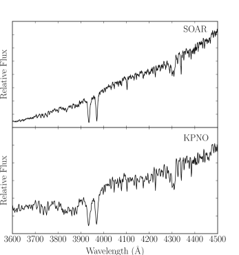
Figure 1: Top Panel: a sample spectrum taken from the SOAR observations. The spectrum is that of a giant from M30, a cluster with ${\rm[Fe/H]}=-2.3$. (Harris 1996; 2010 edition) Bottom Panel: a sample spectrum taken from the KPNO observations. The spectrum is that of a giant from M10, which has an [Fe/H] value of $-1.56$. (Harris 1996; 2010 edition) The CN and CH bands can be seen around 3800 Å and 4300 Å, respectively.

2.3 Reduction

Spectra for each star from the KPNO observations were reduced following standard reduction procedures using the Image Reduction and Analysis Facility (IRAF). The CCD frames were bias and flat-field corrected prior to the extraction of one-dimensional spectra. Initial wavelength calibrations were obtained from the comparison arc exposures accompanying each stellar observation. There is a considerable range in radial velocities among the clusters observed at KPNO. A radial velocity for each star was consequently calculated by cross-correlating the stellar spectrum against a synthetic spectrum of a typical red giant to check for membership. Shifts obtained from the cross-correlation were used to place each spectrum in a stellar rest frame. Spectra were flux calibrated.

For the SOAR observations, a different method was used to reduce the spectra due to a large reflection in the flat-field images obtained from the telescope. To eliminate the reflection, a series of flats were taken at an additional grating angle that moved the reflection to a different location on the detector. The region in the original flat with the reflection was then replaced with a section from the new flat after normalization.

Another issue encountered with the SOAR observations was that the arc lamp exposures for each the program were underexposed. Here a well-exposed arc taken at the start of the night was used to obtain the general shape of the pixel-wavelength solution, which was then applied to the program stars. A cross-correlation between the resulting program spectrum and a synthetic template was then used to shift the observed spectra into the rest frame. A consequence of this approach was the loss of any radial-velocity information. However, all SOAR program stars are believed to be members based on their positions on the color magnitude diagrams of the clusters.

3 Analysis

Carbon and nitrogen abundances were derived for each star by modeling two spectroscopic indices measured from the spectra, one being a CH index covering a strong CH absorption band located at 4300 Å (the so-called $G$ band), with a second index chosen to be sensitive to a CN absorption feature with a bandhead at 3883 Å. The CN index that was measured is denoted $S(3839)$ and was introduced by Norris et al. (1981) specifically for comparing the intensity in the violet CN band at 3883 Å with a nearby redward comparison region of $\lambda\lambda$3883-3916 Å that avoids CN absorption. The $I{\rm(CH)}$ absorption index used employs two pseudo-continuum bandpasses, a blueward region of 4240-4280 Å, and a redward bandpass from 4390 to 4460 Å. The CH feature bandpass itself covers the wavelength range of $\lambda\lambda$4285-4315 Å (Harbeck et al., 2003). In the case of the $I{\rm(CH)}$ absorption index, each bandpass (continuum and feature) were normalized by their width by dividing the sum of the bandpass by its width in angstroms. Equations 1 and 2 show how the $S(3839)$ and $I{\rm(CH)}$ indices were calculated with $F_{X-Y}$ being the total integrated flux between wavelengths $X$ and $Y$.

$$S(3839)=-2.5\log\frac{F_{3846-3883}}{F_{3883-3916}}$$ (1)

$$I{\rm(CH)}=-2.5\log\frac{F_{4285-4315}/30}{0.5(C_{1}+C_{2})}$$ (2)

$$C_{1}=F_{4240-4280}/40$$ (3)

$$C_{2}=F_{4390-4460}/70$$ (4)

The model atmospheres generated for each star were computed using the MARCS program (Gustafsson et al., 2008) and the Synthetic Spectrum Generator (SSG; Bell & Gustafsson, 1978, 1989). Effective temperatures and surface gravities required for the stellar models were derived using the $V-K$ color of a star, the absolute magnitude, and an [Fe/H] value based on cluster membership. The apparent $V$ magnitudes for the program stars came from the sources referenced in Table 1, while the $K_{s}$ magnitudes were taken from the 2MASS catalog (Skrutskie, Cutri, Stiening, et al., 2006). The Harris catalog (Harris 1996; 2010 edition) was the source for the [Fe/H] adopted for each cluster.

Determination of stellar temperatures and surface gravities was done according to the method described in Alonso, Arribas, & Martinez-Roger (1999) and Alonso, Arribas, & Martinez-Roger (2001). The equation in Alonso, Arribas, & Martinez-Roger (2001) that gives the stellar effective temperature as a function of the $V-K$ color uses the Carlos Sanchez Telescope (TCS) photometric system. Thus $V-K$ colors from 2MASS were first converted to the TCS system using the method described in Johnson et al. (2004). The $V-K$ color on the TCS system was then corrected for reddening by subtracting the $E(B-V)$ values from Harris (1996, 2010 edition) multiplied by 2.74, which is the adopted reddening ratio from Prisinzano et al. (2012).

Synthetic spectra were calculated for each effective temperature and $\log g$ with the appropriate [Fe/H] then smoothed to match the observed spectrum for the individual stars. Carbon and nitrogen were adjusted simultaneously to match the CN and CH indices. Due to the role of the CO molecule in setting molecular equilibrium abundances in red giant photospheres, the [O/Fe] abundance used in generating the synthetic spectra for each star is an important constraint. Whenever possible, we used the literature values for any star in our study with measured [O/Fe] abundances (Sneden et al., 2004; Cohen & Melendez, 2005; Carretta et al., 2009a, b; Johnson & Pilachowski, 2012; Boberg et al., 2015, 2016; Rojas-Arriagada et al., 2016; Villanova et al., 2016; Marino et al., 2018). If a star did not have a direct measurement, but belonged to a cluster with other [O/Fe] measurements, we assigned an [O/Fe] equal to the cluster average for that star. In the cases where no measurements were available for a cluster, an [O/Fe] abundance of 0.3 dex was assumed. This value is based on Figure 6 of Carretta et al. (2009a) that shows [O/Fe] measurements for 19 GCs all approximately centered on 0.3 dex. $\xi=2.0$ km s^-1 and ${}^{12}{\rm C}/^{13}{\rm C}=4.0$ were also assumed for the synthetic spectra, which are reasonable estimates for GC RGB stars (e.g., Suntzeff & Smith, 1991; Pavlenko et al., 2003). The resulting carbon abundances are plotted in Fig. 2 as a function of the metallicity of each cluster. The derived [C/Fe] and [N/Fe] values are presented in Table 3.

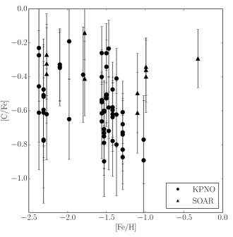
Figure 2: Carbon abundance [C/Fe] vs. [Fe/H] for each star in the KPNO/SOAR sample. The circles indicate stars observed with the KPNO 4 m telescope and triangles are those observed with the SOAR telescope. The error bars represent uncertainties from multiple observations of the same star. There is no clear correlation between [C/Fe] and [Fe/H].

To evaluate our uncertainties of the resulting abundances based on the sensitivity to [O/Fe], [Fe/H], the ${}^{12}{\rm C}/^{13}{\rm C}$ ratio, and errors in temperatures, gravities, and band strengths, we repeated the C and N abundance determinations using different values for these input parameters as shown in Table 2. We chose to vary [O/Fe] by $\pm$ 0.3 dex as this range encompasses the [O/Fe] of most stars observed by Carretta et al. (2009a, b). Maximum uncertainties for effective temperatures based on the method in Alonso, Arribas, & Martinez-Roger (1999) and Alonso, Arribas, & Martinez-Roger (2001) are 150 K, which results in uncertainties in surface gravity of 0.2, so we varied these parameters by these values. For the band strength uncertainties, we subtracted the uncertainty in $I(\rm{CH})$ and added the uncertainty in $S(3839)$ to maximize the effect of these uncertainties since the bands are negatively correlated. A final uncertainty for each star is then calculated by adding the changes from each of these assumptions in quadrature and provided in Table 3. The average change on [C/Fe] and [N/Fe] from each of these parameters for the sample is also given in Table 2, which shows that the greatest sensitivity is to $T_{\rm{eff}}$ and [O/Fe] and demonstrates the importance of our careful selection of [O/Fe] values.

A further check on our methods for assigning parameters such as O abundances comes from comparisons with the study of Martell, Smith, & Briley (2008). We note that our study has nine stars in common with Martell, Smith, & Briley (2008) who determined carbon abundances for RGB stars in GCs through a similar method to ours (matching CN and CH bands with synthetic spectra). We find that for eight of these nine stars our carbon abundances agree within the uncertainties. The one star that does not agree was likely the result of a poor observation by Martell, Smith, & Briley (2008) as it was left out of the main analysis of that paper. This comparison and consistency between the two studies provides additional support that our methods for determining parameters for each star are appropriate.

Table 1: Abundances for program stars

Globular Cluster	[Fe/H]	$V$	$M_{\mathrm{V}}$	$T_{\rm eff}$ (K)	log($g$)	$S(3839)$	$I{\rm(CH)}$	[C/Fe]	[N/Fe]	Telescope
NGC 6362 (1)
4	-0.99	13.32	-1.36	4328	1.36	0.311	0.389	-0.34 $\pm$ 0.17	0.79 $\pm$ 0.12	SOAR
6	-0.99	13.23	-1.45	4216	1.24	0.483	0.402	-0.36 $\pm$ 0.19	1.10 $\pm$ 0.24	SOAR
25	-0.99	13.32	-1.36	4108	1.19	0.228	0.408	-0.40 $\pm$ 0.21	0.78 $\pm$ 0.24	SOAR
NGC 6723 (2)
1-5	-1.1	13.30	-1.54	3942	0.97	0.432	0.396	-0.61 $\pm$ 0.24	1.76 $\pm$ 0.3	SOAR
2-4-62	-1.1	13.38	-1.46	4004	1.06	0.414	0.400	-0.50 $\pm$ 0.23	1.42 $\pm$ 0.25	SOAR
NGC 7099 (M30) (3), (4)
PE-19	-2.27	13.04	-1.6	4537	1.39	0.037	0.255	-0.27 $\pm$ 0.24	1.41 $\pm$ 0.10	SOAR
38	-2.27	13.24	-1.4	4642	1.53	-0.027	0.189	-0.38 $\pm$ 0.29	1.56 $\pm$ 0.11	SOAR
157	-2.27	13.00	-1.64	4419	1.30	-0.014	0.278	-0.32 $\pm$ 0.21	1.15 $\pm$ 0.10	SOAR

Note. — This table is available in its entirety in machine-readable form.

References. — (1)Alcaino (1972), (2)Menzies (1974), (3)Alcaino (1978), (4)Dickens (1972)

Table 2: Sensitivity of the derived [C/Fe] abundance to input parameters for SSG synthetic spectra

Parameter Change	Average $\Delta$[C/Fe]	$\Delta$[N/Fe]
$T_{\rm eff}\pm 150$ K	0.16	0.12
log(g) $\pm$ 0.2	0.03	0.04
$[$O/Fe$]$ $\pm$ 0.3 dex	0.10	0.05
$[$Fe/H$]$ $\pm$ 0.1 dex	0.05	0.03
$S(3839)$ and $I{\rm(CH)}$ $\pm$ 0.01	0.05	0.08
${{}^{12}{\rm C}}/{}{{}^{13}{\rm C}}$ $\sim+10$	0.02	0.02

4 Results

A summary of the carbon abundances derived in this program is shown in Fig. 2, which is a plot of [C/Fe] versus [Fe/H] for each star in the sample (circles for stars observed at KPNO; triangles for stars observed at SOAR). All but one star has ${\rm[C/Fe]}<-0.2$, with some being carbon depleted by as much as ${\rm[C/Fe]}\sim-1.0$. Such non-solar [C/Fe] ratios are signs that carbon has likely been depleted at the surfaces of the cluster giants (halo subdwarfs, for example, more typically have near-solar [C/Fe]; see for example, Laird (1985), Carbon et al. (1987), Gratton et al. (2000)). If GC stars were formed with initial carbon abundances commensurate with those of subdwarfs then the implication of the abundances in Fig. 2 is that a process has been at work within the cluster giants that has brought about a reduction in the surface carbon abundance. Within the context of the interior structure of the GC giants, some physical mechanism has caused carbon-depleted material from the CNO-bi-cycle hydrogen-burning shell to be transported across the radiative region that surrounds the shell and thence carried into the convective envelope, whereupon it is rapidly convected to the surface of the red giant. We colloquially use the term extra mixing to refer to the process that produces these carbon depletions. This refers to a non-convective mixing or mass transport of material across the interior radiative zone of the red giant, i.e., it is a mixing process that acts in addition to the outer convective envelope. Although there may seem to be no pattern to the distribution of points in Fig. 2, there is an underlying dependence of deep mixing on metallicity implicit in these data.

Stellar interior theory indicates that mixing between the base of the convective envelope of a cluster giant and the outer parts of the hydrogen-burning shell can only take place after this shell has burned through a molecular weight discontinuity left within the star at a location corresponding to the deepest inward extent of the base of the convective envelope during evolution up the RGB (Iben, 1965, 1968). The occurrence of this burn through event produces a local maximum in the RGB luminosity function. Taking this conventional theory as being correct, for each of the clusters in our sample the absolute magnitude of the LMLF can be predicted. Through further application of stellar evolution models the time since each star in our sample has evolved through the LMLF can be calculated. Assuming a primordial [C/Fe] for each cluster, a comparison with the observed [C/Fe] values then allows the calculation of a carbon depletion rate on the RGB to be derived for each star. A depletion rate is defined here as the ratio of the change incurred in the [C/Fe] abundance to the time since a star evolved through the LMLF. Such calculated depletion rates can be correlated with metallicity - the prime goal of our project.

The absolute magnitude of the LMLF for each cluster was estimated using a correlation between this magnitude and cluster metallicity that was derived from the cluster data set of Fusi Pecci et al. (1990). The correlation is shown in Fig. 3. A linear interpolation was used with the data from Fusi Pecci et al. (1990) to calculate a value of $M_{\mathrm{V}}$(LMLF) for each cluster in our sample. The LMLF magnitudes from Fusi Pecci et al. (1990), as well as the values derived for the clusters in our sample, are both shown in Fig. 3.

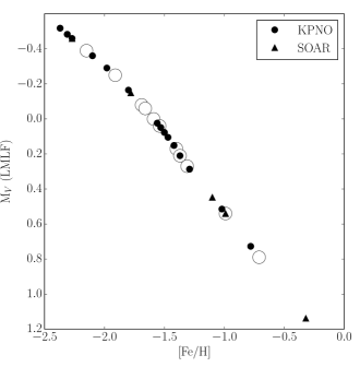
Figure 3: Absolute magnitude of the local maximum in the luminosity function of a globular cluster as a function of metallicity. The data points are taken from Fusi Pecci et al. (1990). The solid circles represent clusters observed as part of the KPNO sample, and the triangles represent clusters observed with the SOAR telescope. Clusters from Fusi Pecci et al. (1990) not in our sample are shown as open circles. The solid lines are linear interpolations between the data points.

Following the method of Martell, Smith, & Briley (2008), we use Yale Y² isochrones (Yi et al., 2001) to determine a characteristic rate for the luminosity evolution, $\Delta M_{\mathrm{V}}/\Delta t$, of stars with metallicities corresponding to each GC in the observational program. A stellar model for a given [Fe/H] was chosen within 0.05 mag of the LMLF from an isochrone calculated with an age of 12 Gyr. This model sets the mass of a 12-Gyr-old star that is evolving through the LMLF for a cluster of the given [Fe/H]. Additional isochrones of greater age were then reviewed until one was found where a model of the appropriate mass had evolved to an absolute magnitude of $M_{\mathrm{V}}=-1.5\pm 0.05$. The age difference, $\Delta t$ between the two isochrones provided a value for the ratio $\Delta M_{\mathrm{V}}/\Delta t$, representing the mean rate at which a star evolves up the RGB past the LMLF in each cluster.

Once a change in magnitude as a function of time had been calculated for each star, a change in carbon abundance as a function of magnitude was determined from (i) the difference in [C/Fe] from an assumed initial solar [C/Fe] and (ii) the difference in absolute magnitude of the star from the LMLF of the cluster. With $\Delta{\rm[C/Fe]}/\Delta M_{\mathrm{V}}$ thereby established for each star in the sample, a value for the carbon depletion rate, $\Delta{\rm[C/Fe]}/\Delta t$, was derived with units of dex per gigayear.

A plot of the carbon depletion rate for each star as a function of metallicity is shown in Fig. 4 with error bars showing the propagated uncertainty that was calculated for our [C/Fe] measurements from Section 3. A correlation with [Fe/H] is evident, and in this sense our result is analogous to that of Martell, Smith, & Briley (2008), whose methodology we have followed so far. However, there is a large spread in the calculated depletion rate at each metallicity, especially around ${\rm[Fe/H]}\sim-1.5$ where the sample is most numerous.

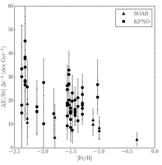
Figure 4: Inferred carbon depletion rate as a function of [Fe/H] for each member of our sample. Members from the SOAR observations are shown as triangles and the KPNO observations are shown as circles. To obtain this diagram the assumption has been made that all stars formed with the same initial solar [C/Fe], which is later modified by deep mixing. A general decrease in the carbon depletion rate is seen with increasing [Fe/H] metallicity, although there is considerable scatter (especially around ${\rm[Fe/H]}\sim-1.5$).

One complication is that in some clusters it is known that there is a relation between CN and CH band strengths among red giants of similar abundance magnitudes (Gratton et al., 2004, and references therein). This translates into a scatter in [C/Fe] at a given $M_{\mathrm{V}}$ in such a way that the [C/Fe] and [N/Fe] are anticorrelated, with CN-strong giants having [C/Fe] abundances lower than those of CN-weak giants of comparable luminosity. Thus one might expect to derive different values of $\Delta{\rm[C/Fe]}/\Delta M_{\mathrm{V}}$ for CN-strong and CN-weak giants. To make allowance for this scatter, [N/Fe], having been derived by simultaneously fitting the $\lambda$3883 CN index, was noted for each star in order to assign it to a nitrogen-rich (CN-strong) or nitrogen-normal (CN-weak) category. If a star is nitrogen-rich, it is taken here to indicate that the star formed from gas that incorporated CN(O)-cycled material through some poorly understood process very early in the cluster history. While the initial CN(O)-cycled material was nitrogen-enhanced, it also had been depleted in carbon; therefore, stars that were formed as nitrogen-rich would generally have had a lower initial carbon abundance than nitrogen-normal stars within the same cluster. An analysis of a histogram of [N/Fe] for the sample showed two peaks clearly separated at [N/Fe] $\sim$ 1.1. Therefore, stars with [N/Fe] greater than 1.1 in this sample were considered nitrogen-rich, and those with [N/Fe] less than 1.1 were considered nitrogen-normal.

A plot of carbon depletion rate versus metallicity is shown in Fig. 5 with the stars indicated as nitrogen-rich or nitrogen-normal. In general, it appears as though nitrogen-rich giants have higher carbon depletion rates than nitrogen-normal ones. However, the carbon depletion rates are likely overestimated for the nitrogen-rich stars because their initial carbon abundances are likely lower than assumed in the calculation of $\Delta$[C/Fe]. If the initial [C/Fe] is lowered to $-0.3$ for the nitrogen-rich stars, the resulting $\Delta$[C/Fe] is reduced as well as the calculated carbon depletion rate. Lowering the carbon depletion rates in the nitrogen-rich stars according to this recipe results in values of $\Delta{\rm[C/Fe]}/\Delta t$ that are plotted versus [Fe/H] in Fig. 6. The scatter in depletion rate at a given [Fe/H] is reduced as compared with the spread seen in Figure 4, particularly around stars in clusters with a metallicity of ${\rm[Fe/H]}\sim-1.5$.

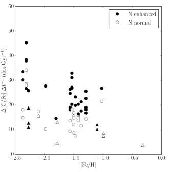
Figure 5: Carbon depletion rate vs. metallicity. Analogous to Fig. 4, except that nitrogen-normal stars are depicted as open circles for the KPNO data and open triangles for the SOAR data. Likewise, filled circles and triangles depict nitrogen-enhanced stars observed at these two telescopes. The error bars are removed for clarity, but are the same as in Fig. 4.

Comparison between Figs. 4 and 6 illustrates the degree to which the inferred carbon depletion rates are dependent upon assuming an initial [C/Fe] for the red giants in our cluster sample. To precisely determine $\Delta{\rm[C/Fe]}/\Delta t$ for a given RGB star, one would need to know the initial [C/Fe] for that star before it began deep mixing. Determining [C/Fe] and [N/Fe] for stars on the main sequence of a cluster, or just before the point of mixing (the subgiant or early giant phase), could provide an estimate for the initial [C/Fe] for nitrogen-rich RGB stars. However, recent studies have shown that in some clusters the [C/Fe] and [N/Fe] abundances of main sequence and early turn-off stars spread over a wide range ($\sim 0.5$ dex) rather than forming a bimodal distribution that could conveniently be identified with nitrogen-rich and nitrogen-normal abundances (e.g., Briley et al. (2004); Cohen, Briley, & Stetson (2005)). Because of the range in initial [C/Fe] and [N/Fe] abundances before mixing has begun, a value for the initial [C/Fe] of any particular star currently in a deep mixing phase on the upper RGB may be difficult to determine. Such uncertainty will inevitably limit the precision with which $\Delta{\rm[C/Fe]}/\Delta t$ can be determined through the type of technique that we have employed in this observational program. The more robust, but more telescope time intensive, approach to deriving $\Delta{\rm[C/Fe]}/\Delta t$ for a particular cluster would be to measure $\Delta{\rm[C/Fe]}/\Delta M_{\mathrm{V}}$ for CN-strong and CN-weak giants separately spanning a large luminosity range on the RGB, similar to what has been done by Suntzeff (1981), Carbon et al. (1982), Trefzger et al. (1983), Langer et al. (1986), Bellman et al. (2001), Shetrone et al. (2010), Kirby et al. (2015), and Gerber et al. (2018) for various clusters.

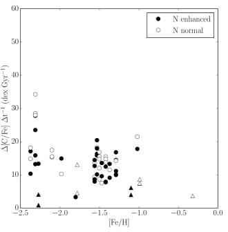
Figure 6: Carbon depletion rate as a function of metallicity after allowing for initial differences in [C/Fe] between nitrogen-rich and nitrogen-normal giants. The carbon depletion rates for the nitrogen-rich giants have been lowered to account for their lower initial carbon abundance. The spread in carbon depletion rates within each cluster is reduced, especially around ${\rm[Fe/H]}\sim-1.5$.

5 Conclusions

We have presented our findings for carbon depletion rates among GC red giants for a range of metallicities following a method similar to Martell, Smith, & Briley (2008). While we were unable to reduce the star-to-star scatter observed by that work, we were able to determine that the scatter is caused by more than variability in mixing rates. We found that this method of determining mixing rates is heavily dependent on the assumed initial carbon abundance for each star. Laird (1985), Carbon et al. (1987), and Gratton et al. (2000) have shown that a solar [C/Fe] value is a reasonable assumption for the initial abundance based on values measured in halo subdwarfs, but the multiple populations now known to exist in most Galactic GCs (see, e.g., Piotto et al., 2015) add complications since the initial carbon abundance will be dependent on the population a RGB star belongs to.

Taking this into consideration, we find the typical rate of carbon depletion to range from $\sim$20 to 50 dex Gyr^-1, with higher rates being found among metal-poorer clusters. Extra mixing has been assumed here to commence when a star evolves through the magnitude corresponding to the LMLF. In the clusters of our sample, the typical time taken to evolve from the $M_{\mathrm{V}}$(LMLF) to the tip of the RGB is $\sim$30-50 Myr (depending on the cluster, with lower metallicity clusters taking less time). If mixing were to continue at the same average rate throughout the entire upper RGB, the total amounts of carbon depletion incurred by GC red giants just prior to the core-helium flash would be $\sim$1.0-1.5 dex dependent upon metallicity. Thus some quite substantial carbon depletion would be anticipated among GC stars as they evolve onto the horizontal branch. We also note that the complications from multiple populations mean that more observationally intensive methods that measure large samples of red giants in each cluster will be needed to separate changes caused by deep mixing from those caused by multiple populations.

6 Acknowledgements

We would like to thank Roger A. Bell for making the SSG program available to us. M. M. Briley and G. H. Smith gratefully acknowledge support by the National Science Foundation through the grants AST-0908924 and AST-0908757, respectively.

This publication makes use of data products from the Two Micron All Sky Survey, which is a joint project of the University of Massachusetts and the Infrared Processing and Analysis Center/California Institute of Technology, funded by the National Aeronautics and Space Administration and the National Science Foundation.

References

- Alcaino (1972) Alcaino, G. 1972, A&A, 16, 220
- Alcaino (1978) Alcaino, G. 1978, A&AS, 33, 185
- Alonso, Arribas, & Martinez-Roger (1999) Alonso, A., Arribas, S., & Martinez-Roger, C. 1999, A&AS, 140, 261
- Alonso, Arribas, & Martinez-Roger (2001) Alonso, A., Arribas, S., & Martinez-Roger, C. 2001, A&A, 376, 1039
- Angelou et al. (2011) Angelou, G. C., Church, R. P., Stancliffe, R. J., Lattanzio, J. C., & Smith, G. H. 2011, ApJ, 728, 79
- Angelou et al. (2012) Angelou, G. C., Stancliffe, R. J., Church, R. P., Lattanzio, J. C., & Smith, G. H. 2012, ApJ, 749, 128
- Arp (1955) Arp, H. C. 1955, AJ, 60, 317
- Asplund et al. (2009) Asplund, M., Grevesse, N., Sauval, A. J., & Scott, P. 2009, ARA&A, 47, 481
- Bell & Gustafsson (1978) Bell, R. A., & Gustafsson, B. 1978, A&AS, 34, 229
- Bell & Gustafsson (1989) Bell, R. A., & Gustafsson, B. 1989, MNRAS, 236, 653
- Bellman et al. (2001) Bellman, S., Briley, M. M., Smith, G. H., & Claver, C. F. 2001, PASP, 113, 326
- Boberg et al. (2015) Boberg, O. M., Friel, E. D., & Vesperini, E. 2015, ApJ, 804, 109
- Boberg et al. (2016) Boberg, O. M., Friel, E. D., & Vesperini, E. 2016, ApJ, 824, 5
- Briley et al. (2004) Briley, M. M., Harbeck, D., Smith, G. H., & Grebel, E. K. 2004, AJ, 127, 1588
- Buonanno et al. (1983) Buonanno, R., Buscema, G., Corsi, C. E., et al. 1983, A&AS, 53, 1
- Buonanno et al. (1983) Buonanno, R., Buscema, G., Corsi, C. E., Iannicola, G., & Fusi Pecci, F. 1983, A&AS, 51, 83
- Cantiello & Langer (2010) Cantiello, M., & Langer, N. 2010, A&A, 521, A9
- Carbon et al. (1987) Carbon, D. F., Barbuy, B., Kraft, R. P., Friel, E. D., & Suntzeff, N. B. 1987, PASP, 99, 335
- Carbon et al. (1982) Carbon, D. F., Langer, G. E., Butler, D., et al. 1982, ApJS, 49, 207
- Carretta et al. (2009a) Carretta, E., Bragaglia, A., Gratton, R., et al. 2009, A&A, 505, 117
- Carretta et al. (2009b) Carretta, E., Bragaglia, A., Gratton, R., & Lucatello, S. 2009, A&A, 505, 139
- Cayrel de Strobel et al. (2001) Cayrel de Strobel, G., Soubiran, C., & Ralite, N. 2001, A&A, 373, 159
- Charbonnel, Brown, & Wallerstein (1998) Charbonnel, C., Brown, J. A., & Wallerstein, G. 1998, A&A, 332, 204
- Charbonnel & Zahn (2007) Charbonnel, C., & Zahn, J.-P. 2007, A&A, 476, L29
- Cohen, Briley, & Stetson (2005) Cohen, J. G., Briley, M. M., & Stetson, P. B. 2005, AJ, 130, 1177
- Cohen & Melendez (2005) Cohen, J. G., & Melendez, J. 2005, AJ, 129, 1607
- Cuffey (1961) Cuffey, J. 1961, PGLO, 45, 364
- Dékány & Kovács (2009) Dékány, I., & Kovács, G. 2009, A&A, 507, 803
- Denissenkov & Pinsonneault (2008) Denissenkov, P. A., & Pinsonneault, M. 2008, ApJ, 684, 626
- Denissenkov & Tout (2000) Denissenkov, P. A., & Tout, C.A 2000, MNRAS, 316, 395
- Denissenkov & VandenBerg (2003) Denissenkov, P. A., & VandenBerg, D. A. 2003, ApJ, 593, 509
- Denissenkov & Weiss (1996) Denissenkov, P. A., & Weiss, A. 1996, A&A, 308, 773
- Dickens (1972) Dickens, R. J. 1972, MNRAS, 157, 299
- Eggleton, Dearborn, & Lattanzio (2006) Eggleton, P. P., Dearborn, D. S. P., & Lattanzio, J. C. 2006, Sci, 314, 1580
- Fusi Pecci et al. (1990) Fusi Pecci, F., Ferraro, F. R., Crocker, D. A., Rood, R. T., & Buonanno, R. 1990, A&A, 238, 95
- Gerber et al. (2018) Gerber, J. M., Friel, E. D., & Vesperini, E. 2018, AJ, 156, 6
- Gratton et al. (2004) Gratton, R., Sneden, C., & Carretta, E. 2004, ARA&A, 42, 385
- Gratton et al. (2000) Gratton, R. G., Sneden, C., Carretta, E., & Bragaglia, A. 2000, å, 354, 169
- Gustafsson et al. (2008) Gustafsson, B., Edvardsson, B., Eriksson, K., et al. 2008, A&A, 486, 951
- Harbeck et al. (2003) Harbeck, D., Smith, G. H., & Grebel, E. K. 2003, AJ, 125, 197
- Harris, & Racine (1973) Harris, W. E., & Racine, R. 1973, AJ, 78, 242
- Harris et al. (1976) Harris, W. E., Racine, R., & de Roux, J. 1976, ApJS, 31, 13
- Harris (1996) Harris, W. E. 1996, AJ, 112, 1487
- Hatzidimitriou et al. (2004) Hatzidimitriou, D., Antoniou, V., Papadakis, I., et al. 2004, MNRAS, 348, 1157
- Henkel et al. (2017) Henkel, K., Karakas, A. I., & Lattanzio, J. C. 2017, MNRAS, 469, 4600
- Iben (1965) Iben, I., Jr. 1965, ApJ, 142, 1447
- Iben (1968) Iben, I., Jr. 1968, ApJ, 154, 581
- Johnson et al. (2004) Johnson, C. I., Kraft, R. P., Pilachowski, C. A., et al. 2005, PASP, 117, 1308
- Johnson & Pilachowski (2012) Johnson, C. I., & Pilachowski, C. A. 2012, ApJ, 754, L38
- Keller et al. (2001) Keller, L. D., Pilachowski, C. A., & Sneden, C. 2001, AJ, 122, 2554
- Kirby et al. (2015) Kirby, E. N., Guo, M., Zhang, A. J., et al. 2015, ApJ, 801, 125
- Lagarde et al. (2012) Lagarde, N., Decressin, T., Charbonnel, C., et al. 2012, A&A, 543, A108
- Laird (1985) Laird, J. B. 1985, ApJ, 289, 556
- Langer et al. (1986) Langer, G. E., Kraft, R. P., Carbon, D. F., Friel, E., & Oke, J. B. 1986, PASP, 98, 473
- Marino et al. (2018) Marino, A. F., Yong, D., Milone, A. P., et al. 2018, ApJ, 859, 81
- Martell, Smith, & Briley (2008) Martell, S. L., Smith, G. H., & Briley, M. M. 2008, AJ, 136, 2522
- Menzies (1974) Menzies, J. 1974, MNRAS, 168, 177
- Meszaros et al. (2008) Mészáros, S., Dupree, A. K., & Szentgyorgyi, A. 2008, AJ, 135, 1117
- Mészáros et al. (2009) Mészáros, S., Dupree, A. K., & Szalai, T. 2009, AJ, 137, 4282
- Norris et al. (1981) Norris, J., Cottrell, P. L., Freeman, K. C., & Da Costa, G. S. 1981, ApJ, 244, 205
- Palacios et al. (2006) Palacios, A., Charbonnel, C., Talon, S., & Siess, L. 2006, A&A, 453, 261
- Pavlenko et al. (2003) Pavlenko, Y. V., Jones, H. R. A., & Longmore, A. J. 2003, MNRAS, 345, 311
- Piotto et al. (2015) Piotto, G., Milone, A. P., Bedin, L. R., et al. 2015, AJ, 149, 91
- Prisinzano et al. (2012) Prisinzano, L., Micela, G., Sciortino, S., Affer, L., Damiani, F., 2012, A&A 546, 9
- Racine (1971) Racine, R. 1971, AJ, 76, 331
- Rey et al. (1998) Rey, S.-C., Lee, Y.-W., Byun, Y.-I., & Chun, M.-S. 1998, AJ, 116, 1775
- Rojas-Arriagada et al. (2016) Rojas-Arriagada, A., Zoccali, M., Vásquez, S., et al. 2016, A&A, 587, A95
- Sandage (1953) Sandage, A. R. 1953, AJ, 58, 61
- Sandage & Walker (1955) Sandage, A. R., & Walker, M. F. 1955, AJ, 60, 230
- Sandage & Katem (1964) Sandage, A., & Katem, B. 1964, ApJ, 139, 1088
- Sandage et al. (1977) Sandage, A., Katem, B., & Johnson, H. L. 1977, AJ, 82, 389
- Sandquist & Bolte (2004) Sandquist, E. L., & Bolte, M. 2004, ApJ, 611, 323
- Sarajedini & Layden (1997) Sarajedini, A., & Layden, A. 1997, AJ, 113, 264
- Sawyer Hogg (1973) Sawyer Hogg, H. 1973, Publications of the David Dunlap Observatory, 3, 6
- Shetrone et al. (2010) Shetrone, M., Martell, S. L., Wilkerson, R., et al. 2010, AJ, 140, 1119
- Skrutskie, Cutri, Stiening, et al. (2006) Skrutskie, M. F., Cutri, R. M., Stiening, R., et al. 2006, AJ, 131, 1163
- Sneden et al. (2004) Sneden, C., Kraft, R. P., Guhathakurta, P., Peterson, R. C., & Fulbright, J. P. 2004, AJ, 127, 2162
- Suda & Fujimoto (2006) Suda, T., & Fujimoto, M. Y. 2006, ApJ, 643, 897
- Suntzeff (1981) Suntzeff, N. B. 1981, ApJS, 47, 1
- Suntzeff & Smith (1991) Suntzeff, N. B., & Smith, V. V. 1991, ApJ, 381, 160
- Sweigart & Mengel (1979) Sweigart, A. V., & Mengel, J. G. 1979, ApJ, 229, 624
- Szigeti et al. (2018) Szigeti, L., Mészáros, S., Smith, V. V., et al. 2018, MNRAS, 474, 4810
- Trefzger et al. (1983) Trefzger, D. V., Langer, G. E., Carbon, D. F., Suntzeff, N. B., & Kraft, R. P. 1983, ApJ, 266, 144
- Villanova et al. (2016) Villanova, S., Monaco, L., Moni Bidin, C., & Assmann, P. 2016, MNRAS, 460, 2351
- Weiss et al. (2000) Weiss, A., Denissenkov, P. A., & Charbonnel, C. 2000, A&A, 356, 181
- Yi et al. (2001) Yi, S., Demarque, P., Kim, Y.-C., et al. 2001, ApJS, 136, 417
- Zoccali et al. (1999) Zoccali, M., Cassisi, S., Piotto, G., Bono, G., & Salaris, M. 1999, ApJ, 518, L49