Understanding Detailed Balance for an Electron–Radiation System Through Mixed Quantum–Classical Electrodynamics

Abstract

We investigate detailed balance for a quantum system interacting with thermal radiation within mixed quantum–classical theory. For a two-level system coupled to classical radiation fields, three semiclassical methods are benchmarked: (1) Ehrenfest dynamics over-estimate the excited state population at equilibrium due to the failure of capturing vacuum fluctuations. (2) The coupled Maxwell–Bloch equations, which supplement Ehrenfest dynamics by damping at the full golden rule rate, under-estimate the excited state population due to double-counting of the self-interaction effect. (3) Ehrenfest+R dynamics recover detailed balance and the correct thermal equilibrium by enforcing the correct balance between the optical excitation and spontaneous emission of the quantum system. These results highlight the fact that, when properly designed, mixed quantum–classical electrodynamics can simulate thermal equilibrium in the field of nanoplasmonics.

I Introduction

For a quantum system in contact with a thermal bath at temperature $T$, detailed balance implies that the equilibrium population of quantum state $i$ with energy $E_{i}$ should satisfy the Boltzmann distribution: $P_{i}\propto e^{-\beta E_{i}}$ where $\beta=1/k_{B}T$ and $k_{B}$ is the Boltzmann constant. This principle of detailed balance is one of the most fundamental aspects underlying chemical kinetics and absorption/emission of radiation(Onsager, 1931; Loudon, 2000; Milonni, 2013). For example, the Onsager reciprocal relations in thermodynamics and Einstein’s famous A and B coefficients in his theory of radiation are both based on detailed balance. Thus, maintaining detailed balance is considered an important measure of validity for any theoretical model of coupled system–bath equilibrium. For decades, achieving the correct equilibrium populations has been a long-standing challenge for semiclassical simulations of electronic–nuclear dynamics(Parandekar and Tully, 2005, 2006; Schmidt, Parandekar, and Tully, 2008; Bastida et al., 2007) and electron–radiation interactions(Milonni, 1976; Slavcheva et al., 2002; Ruggenthaler et al., 2014).

Within the field of electronic–nuclear dynamics, semiclassical simulations rely on a mixed quantum–classical framework that treats the electronic/molecular system with quantum mechanics and the bath degrees of freedom with classical mechanics. Within this framework, recovering detailed balance requires both energy conservation of the entire system and the correct energy exchange rates between the quantum and classical subsystems. Already a decade ago, Tully showed that the equilibrium populations of a coupled electron–nuclei problem as attained by Ehrenfest dynamics deviates from the correct Boltzmann distribution when the nuclear bath temperature decreases(Parandekar and Tully, 2005). This deviation can be attributed to the deficiency of Ehrenfest mean-field theory to properly account for non-adiabatic electronic transitions (even though the total energy is conserved)(Parandekar and Tully, 2006). To capture non-adiabatic effects within a mixed quantum–classical framework, the most common solution is either to design a stochastic mechanism to simulate electronic transitions, such as surface hopping algorithms(Tully, 1990, 1998; Schmidt, Parandekar, and Tully, 2008; Jain and Subotnik, 2015; Bellonzi, Jain, and Subotnik, 2016; Sifain, Wang, and Prezhdo, 2016), or to introduce binning as in the symmetrical quasi-classical (SQC) approach(Cotton and Miller, 2013; Miller and Cotton, 2015), both of which can almost recover detailed balance for coupled electron–nuclei equilibrium.

If we now turn to electron–radiation dynamics, the equations of motion within a mixed quantum–classical framework are formally similar to those for electronic–nuclear dynamics. And yet, because thermal radiation fields cannot be properly modeled by classical electrodynamics (due to the notorious blackbody radiation problem), the applicability of Tully’s argument to electron–radiation equilibrium is unclear. And more generally, the feasibility of semiclassical techniques to model electrodynamics and to reach detailed balance quantitatively remains an open question. While many semiclassical schemes for electrodynamics have been introduced(Milonni, 1976; Miller, 1978), including the coupled Maxwell–Bloch equations(Castin and Mo/lmer, 1995; Ziolkowski, Arnold, and Gogny, 1995; Slavcheva et al., 2002), mean-field Ehrenfest dynamics(Li et al., 2018; Li, Chen, and Subotnik, 2019; Hoffmann et al., 2018, 2019), Ehrenfest+R method(Chen et al., 2019a, b, c), and quantum electrodynamical density functional theory (QEDFT)(Ruggenthaler et al., 2014; Flick et al., 2017; Ruggenthaler et al., 2018), the capacity of these semiclassical approaches to recover detailed balance has never been fully benchmarked. It is a common presumption that mixed quantum–classical electrodynamics cannot satisfy detailed balance due to the failure of classical electrodynamics to describe the blackbody radiation spectrum—modeling thermal radiation fields classically should inevitably lead to the incorrect Rayleigh–Jeans spectrum(Boyer, 1969; Milonni, 1976, 2013).

Nevertheless, Boyer recently showed that detailed balance can be achieved by considering a fully classical model composed of a classical charged harmonic oscillator coupled to a set of classical electromagnetic (EM) fields(Boyer, 2018). Boyer’s analysis is based on relativistic classical mechanics and random electrodynamics theory that characterizes the fluctuations of thermal radiation using an ensemble of classical EM fields with a random phase(Boyer, 1969, 1975). As shown by Boyer, this classical model of thermal radiation fields can overcome the failure of classical electrodynamics and recover the correct Planck spectrum and zero-point energy(Boyer, 1969, 1976, 1975, 2016) . As such, there is at least one example for how classical electrodynamics can recover the quantum blackbody radiation without invoking the quantization of light as photons.

In this paper, our goal is to employ Boyer’s framework for classically modeling thermal radiation fields and then evaluate the capacity of various mixed quantum–classical methods to recover detailed balance for the electron–radiation equilibrium; note that, unlike Boyer, we will not invoke relativity but rather treat the electronic subsystem with quantum mechanics. Our approach will be to model an electronic two-level system (TLS) coupled to a bath of incoming radiation EM fields at temperature $T$ and then to compare the equilibrium population with the Boltzmann distribution. This paper is organized as follows. In Sec. II, we set up the model Hamiltonian and formulate the boundary conditions for thermal radiation fields. In Sec. III, we briefly review three semiclassical approaches for electron–radiation dynamics. In Sec. IV, we compare the mixed quantum–classical equilibrium as attained by these three different semiclassical models against the correct Boltzmann distribution. We conclude with an outlook for the future in Sec. V.

For notation, we use a bold symbol to denote a space vector $\mathbf{r}=x\boldsymbol{\epsilon}_{x}+y\boldsymbol{\epsilon}_{y}+z\boldsymbol{\epsilon}_{z}$ where $\boldsymbol{\epsilon}$ denotes a unit vector in Cartesian coordinate. We use $\int dv=\int dxdydz$ for integration over 3D space. We work below in SI units.

II The Hamiltonian and boundary conditions

For a model of electron–radiation equilibrium, we consider an electronic TLS coupled to thermal radiation fields in a 3D space. The TLS Hamiltonian is $\widehat{H}_{s}=\hbar\omega_{0}\left|e\right\rangle\left\langle e\right|$ where the ground state $\left|g\right\rangle$ and the excited state $\left|e\right\rangle$ are separated by an energy difference $\hbar\omega_{0}$. For a quantum electrodynamics (QED) description, the TLS is coupled to a set of photon fields that describe thermal radiation fields. Such a model should reach thermal equilibrium when the optical excitation by thermal radiation fields are balanced against the spontaneous emission of the TLS. In the end, the equilibrium populations should follow the Boltzmann distribution (obeying the principle of detailed balance)

$$P_{e}/P_{g}=e^{-\beta\hbar\omega_{0}}.$$ (1)

In general, recovering detailed balance requires an accurate treatment of spontaneous emission. It is well-known that, in QED, spontaneous emission includes two subprocesses: self-interaction and the vacuum fluctuations(Dalibard, Dupont-Roc, and Cohen-Tannoudji, 1982, 1984). Self-interaction is the subprocess induced by the emitted field interacting back with the TLS. The vacuum fluctuations are purely quantum effects that arise from the zero-point energy of the quantum EM fields inducing decay of the TLS.

II.1 Semiclassical Electronic Hamiltonian

For mixed quantum–classical electrodynamics, the TLS is described by an electronic reduced density matrix $\rho\left(t\right)$ while the EM fields, $\mathbf{E}\left(\mathbf{r},t\right)$ and $\mathbf{B}\left(\mathbf{r},t\right)$, are classical. The electric dipole coupling is $\widehat{V}\left(t\right)=-\int\mathrm{d}v\widehat{\mathbf{P}}\left(\mathbf{r}\right)\cdot\mathbf{E}\left(\mathbf{r},t\right)$, which couple the TLS to the total electric field. The polarization density operator of the TLS is defined as $\widehat{\mathbf{P}}\left(\mathbf{r}\right)=\mathbf{d}\left(\mathbf{r}\right)\left(\left|e\right\rangle\left\langle g\right|+\left|g\right\rangle\left\langle e\right|\right)$. We assume that the polarization density takes the form $\mathbf{d}\left(\mathbf{r}\right)=\mu\frac{2e^{-r^{2}/2\sigma^{2}}}{\left(2\pi\sigma^{2}\right)^{3/2}}\boldsymbol{\epsilon}_{z}$ where $\left|\mathbf{r}\right|=r$. Here, $\mu$ is the magnitude of the transition dipole moment and $\sigma$ represents the length scale of the TLS. Note that, for simplicity, we set the polarization to be along the $z$ direction. In practice, we usually make the long-wavelength approximation, assuming that the wavelength of the dominant absorption/emission mode ($2\pi c/\omega_{0}$) is much larger than the size of the TLS (usually on the order of a Bohr radius). With this assumption, we can approximate the polarization density as a point dipole, i.e. $\mathbf{d}\left(\mathbf{r}\right)\rightarrow\mu\delta^{3}\left(r\right)\boldsymbol{\epsilon}_{z}$. For the TLS in vacuum, the spontaneous emission rate is given by the Fermi’s golden rule (FGR) rate, $\kappa=\mu^{2}\omega_{0}^{3}/3\pi\hbar\epsilon_{0}c^{3}$.

Explicitly, the semiclassical electronic Hamiltonian in matrix form reads

$$\widehat{H}^{\mathrm{el}}=\widehat{H}_{s}+\widehat{V}\left(t\right)=\left(\begin{array}[]{cc}0&v\left(t\right)\\ v\left(t\right)&\hbar\omega_{0}\end{array}\right),$$ (2)

where the electric dipole coupling is $v\left(t\right)=-\mu\boldsymbol{\epsilon}_{z}\cdot\mathbf{E}\left(0,t\right)$. Here, we can decompose the total electric field as $\mathbf{E}=\mathbf{E}_{\mathrm{in}}+\mathbf{E}_{\mathrm{scatt}}$ in terms of the incoming thermal radiation fields ($\mathbf{E}_{\mathrm{in}}$) and the scattered field ($\mathbf{E}_{\mathrm{scatt}}$) generated by the stimulated and spontaneous emission processes. In the end, the electric dipole coupling includes two terms: (i) the self-interaction term $\mu\boldsymbol{\epsilon}_{z}\cdot\mathbf{E}_{\mathrm{scatt}}\left(0,t\right)$ and (ii) the optical excitation term $\mu\boldsymbol{\epsilon}_{z}\cdot\mathbf{E}_{\mathrm{in}}\left(0,t\right)$. As is common, we will assume that the effects of these two processes are essentially independent(Cohen-Tannoudji, Dupont-Roc, and Grynberg, 1998).

II.2 Boundary Conditions: Thermal Radiation as Random Electromagnetic Fields

The optical excitation term $\mu\boldsymbol{\epsilon}_{z}\cdot\mathbf{E}_{\mathrm{in}}\left(0,t\right)$ represents the coupling between the TLS and the incoming classical EM fields. As discussed in the introduction, we will employ Boyer’s random electrodynamical model to simulate thermal radiation fields.

As it was originally formulated(Boyer, 1969), random electrodynamics constitute a classical model of thermal radiation fields in terms of a sum over transverse plane waves with a random phase in 3D space (see Eq. (5)). These transverse plane waves follow homogeneous Maxwell equations: $\frac{\partial}{\partial t}\mathbf{B}_{\mathrm{in}}=-\boldsymbol{\nabla}\times\mathbf{E}_{\mathrm{in}}$, $\frac{\partial}{\partial t}\mathbf{E}_{\mathrm{in}}=c^{2}\boldsymbol{\nabla}\times\mathbf{B}_{\mathrm{in}}$. With this random electrodynamical model of thermal radiation fields, the optical excitation term for the electric dipole coupling can be written as a sum over harmonic oscillators with discrete frequency modes (see Appendix A)

$$\mu\boldsymbol{\epsilon}_{z}\cdot\mathbf{E}_{\mathrm{in}}\left(0,t\right)=\sum_{\omega}\mu A\left(\omega,\beta\right)\cos\left[\omega t+\theta_{\omega}\right].$$ (3)

The random phase $\theta_{\omega}\in\left[0,2\pi\right)$ is chosen independently for each frequency $\omega$. Here, the coupling strength for frequency mode $\omega$ is determined by the spectrum

$$\left|A\left(\omega,\beta\right)\right|^{2}=\frac{2\hbar}{3\pi^{2}\epsilon_{0}c^{3}}\frac{\omega^{3}}{e^{\beta\hbar\omega}-1}d\omega,$$ (4)

which corresponds to the true QM energy density within the frequency range $\left(\omega,\omega+d\omega\right)$, though ignoring zero-point energy.

Finally, we emphasize that random electrodynamics theory exploits an ensemble of classical EM fields to simulate the statistical variations of a quantum electrodynamical field. We denote $\left\langle\cdot\right\rangle_{\theta}$ as an average with respect to the random phase $\{\theta_{\omega}\}$. For example, the radiation energy density can be evaluated by $\frac{\epsilon_{0}}{2}\langle\mathbf{E}_{\mathrm{in}}^{2}\rangle_{\theta}+\frac{1}{2\mu_{0}}\langle\mathbf{B}_{\mathrm{in}}^{2}\rangle_{\theta}=\sum_{\omega}U\left(\omega,\beta\right)/V$ and the total electric field is $\langle\mathbf{E}_{\mathrm{in}}\rangle_{\theta}=0$ due to the random phase cancellation. In what follows, we will run multiple trajectories with $\{\theta_{\omega}\}$ chosen randomly and average over those trajectories to evaluate physical observables, such as the average density matrix $\langle\rho\rangle_{\theta}$.

III Mixed Quantum–Classical Electrodynamics

In this section, we briefly review three semiclassical methods for simulating electron–radiation dynamics: (1) Ehrenfest dynamics, (2) the coupled Maxwell–Bloch equations, and (3) the Ehrenfest+R approach. While these methods treat the optical excitation by the incoming thermal radiation fields in the same manner, the incorporation of spontaneous emission effects for the TLS is considered at different levels of accuracy(Li, Chen, and Subotnik, 2019). Since we are interested in the equilibrium population, we focus on the equation of motion for the TLS below.

III.1 Ehrenfest dynamics

Ehrenfest dynamics is the most straightforward, mean–field semiclassical ansatz for electrodynamics(Li et al., 2018). The density matrix of the TLS evolves according to the Liouville equation: $\dot{\rho}=-\frac{i}{\hbar}[\widehat{H}^{\mathrm{el}},\rho]$. The scattered EM fields follow the inhomogeneous Maxwell’s equations: $\frac{\partial}{\partial t}\mathbf{B}_{\mathrm{scatt}}=-\boldsymbol{\nabla}\times\mathbf{E}_{\mathrm{scatt}}$, $\frac{\partial}{\partial t}\mathbf{E}_{\mathrm{scatt}}=c^{2}\boldsymbol{\nabla}\times\mathbf{B}_{\mathrm{scatt}}-\mathbf{J}/\epsilon_{0}$. Here, the current source $\mathbf{J}=\frac{\partial}{\partial t}\text{Tr}\{\rho\widehat{\mathbf{P}}\}$ is generated by the average polarization of the electronic system. Within Ehrenfest dynamics, the total energy of the TLS and the scatted EM fields is conserved. However, as shown in Refs. Li et al., 2018; Chen et al., 2019a, Ehrenfest dynamics completely ignore the effects of vacuum fluctuations and fail to capture spontaneous emission quantitatively. More specifically, for a TLS in vacuum, the population decay rate is $k_{\mathrm{Eh}}(t)=\kappa\rho_{gg}(t)$, i.e. Ehrenfest dynamics tend to be more accurate in the weak excitation limit ($\rho_{gg}\rightarrow 1$, $\rho_{ee}\rightarrow 0$) than in the strong excitation limit ($\rho_{gg}\rightarrow 0$, $\rho_{ee}\rightarrow 1$).

III.2 Coupled Maxwell–Bloch equations

The most common scheme to improve Ehrenfest dynamics is to add some phenomenological dissipation to the Liouville equation: $\dot{\rho}=-\frac{i}{\hbar}[\widehat{H}^{\mathrm{el}},\rho]+{\cal L}_{\mathrm{SE}}[\rho]$ (forming the so-called the coupled Maxwell–Bloch equations(Castin and Mo/lmer, 1995; Ziolkowski, Arnold, and Gogny, 1995)) while the scattered EM fields follow the same equations of motion as Ehrenfest dynamics. The dissipation term takes the form of a Lindblad operator: ${\cal L}_{\mathrm{SE}}[\rho]=\kappa\left(\widehat{a}\rho\widehat{a}^{\dagger}-\frac{1}{2}\widehat{a}^{\dagger}\widehat{a}\rho-\frac{1}{2}\rho\widehat{a}^{\dagger}\widehat{a}\right)$ where $\widehat{a}=\left|g\right\rangle\left\langle e\right|$. Note that the full FGR rate $\kappa$ is used in this phenomenological dissipation. The Lindblad operator can be derived from a QED calculation to describe the overall effects of spontaneous emission.

Unfortunately, naively supplementing Ehrenfest dynamics by this phenomenological damping at the full FGR rate causes many disadvantages for the coupled Maxwell–Bloch equations. First, the total energy of the TLS and the radiation fields is not conserved: there is no EM field emission corresponding to the additional dissipation of the TLS. Second, the effect of the self-interaction is double-counted: the phenomenological Lindblad operator with the FGR rate ($\kappa$) ignores the fact that self-interaction has already been included in Ehrenfest dynamics and only the vacuum fluctuations must be addressed. As has been shown recently(Li, Chen, and Subotnik, 2019), this naive implementation of the coupled Maxwell–Bloch equations almost always over-estimates the population decay rate of the TLS.

III.3 Ehrenfest+R approach

In contract to the coupled Maxwell–Bloch equations, the Ehrenfest+R approach correctly adds only the effect of vacuum fluctuations on top of the Ehrenfest dynamics(Chen et al., 2019a). Explicitly, the +R correction enforces three effects: (1) population relaxation, which adjusts the electronic population to recover spontaneous emission, (2) stochastic dephasing, which introduces a stochastic random phase to the electronic wavefunction, (3) EM field rescaling, which enforces total energy conservation. A detailed implementation of the Ehrenfest+R method is presented in Ref. Chen et al., 2019a; Li, Chen, and Subotnik, 2019.

Now, we emphasize that, within Ehrenfest+R dynamics, the scattered EM fields are described on the same footing as the incoming thermal radiation within random electrodynamics. Since the stochastic random phase $\phi$ is introduced by the +R correction, the scattered EM fields in Ehrenfest+R dynamics constitute an ensemble of classical EM fields. Thus, in the end, when evaluating physical observables, we must average over both $\theta$ (from thermal radiation) and $\phi$ (from the +R correction). For example, if we use an electronic wavefunction to describe the TLS $\left|\psi\left(t\right)\right\rangle=c_{g}\left(t\right)\left|g\right\rangle+c_{e}\left(t\right)\left|e\right\rangle$, the excited state population of the TLS $P_{e}\left(t\right)=\langle\left|c_{e}\left(t\right)\right|^{2}\rangle_{\phi}\rangle_{\theta}$.

IV Results and Discussion

To reach thermal equilibrium between the TLS and the incoming radiation fields, we simulate the dynamics of the TLS for long time ($t=200/\kappa$). We vary the temperature of the thermal radiation ($k_{B}T=1/\beta$) and compare the excited state populations at equilibrium with the Boltzmann distribution: $P_{e}=1/(1+e^{\beta\hbar\omega_{0}})$. Here, we choose $\kappa\ll\omega_{0}$ so as to operate in the FGR regime. The coupling strength $A\left(\omega,\beta\right)$ is discretized by $51$ modes with $d\omega=\kappa/300$ near $\omega_{0}$. For each $\beta$, we run $2000$ trajectories for convergence.

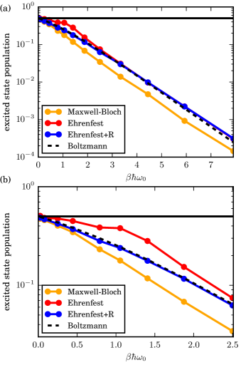
Figure 1: Equilibrium populations of the excited state of the TLS as a function of inverse temperature parameter $\beta\hbar\omega_{0}$. The dashed black lines are the correct Boltzmann distribution. The solid black lines correspond to the saturate population at infinite temperature ($P_{e}=P_{g}=0.5$). The solid circles are the average data obtained by Ehrenfest dynamics (colored red), the coupled Maxwell–Bloch equations (colored orange), and the Ehrenfest+R approach (colored blue). (a) For a large range of temperature, Ehrenfest+R dynamics recover the correct Boltzmann distribution. The coupled Maxwell–Bloch equations almost always under-estimate equilibrium population due to the double-counting of the self-interaction. Surprisingly, Ehrenfest dynamics results agree with the correct Boltzmann distribution at low temperature. (b) In the high temperature regime, Ehrenfest dynamics over-estimate the excited state population due to the failure to fully recover spontaneous emission. For all regimes, Ehrenfest+R dynamics can achieve detailed balance.

Fig. 1(a) shows that Ehrenfest dynamics can recover the Boltzmann distribution for a large range of temperature. Surprisingly, Ehrenfest dynamics results turn out to be more accurate when $\beta$ become larger (low temperature). This observation is the opposite of Tully’s analysis for electron–nuclei equilibrium(Parandekar and Tully, 2005). To rationalize this unexpected temperature dependence, we note that, within the regime of electron–nuclei interactions, one can separate the system–bath coupling strength from the temperature of the bath. By contrast, for electron–radiation interactions, the coupling strength $A\left(\omega,\beta\right)$ itself depends on the temperature of the radiation fields and low temperature generally leads to weak excitation. Now, if we recall that Ehrenfest dynamics can almost recover spontaneous emission for a weakly excited TLS(Li et al., 2018; Li, Chen, and Subotnik, 2019) (because the overall effect of spontaneous emission is dominated by the effect of self-interaction), we must conclude that, at low temperature, excitation of the TLS by thermal radiation will be balanced by the Ehrenfest decay rate (that is almost the correct spontaneous emission rate).

Next, as shown in Fig. 1(b), at high temperature, the equilibrium population obtained by Ehrenfest dynamics is larger than the Boltzmann distribution. At high temperature, the TLS is strongly excited by the incoming thermal radiation and the effects of vacuum fluctuations become more important for spontaneous emission. And thus, due to the failure of Ehrenfest dynamics to include vacuum fluctuations, the Ehrenfest decay rate will be insufficient to balance with the incoming thermal radiation. As a result, Ehrenfest dynamics predict equilibrium populations that are too large and do not satisfy detailed balance.

Now, we turn our attention to the results of the coupled Maxwell–Bloch equations. Due to the double-counting of the self-interaction effect, the coupled Maxwell–Bloch equations almost always produce a smaller equilibrium population than the Boltzmann distribution. Following a similar analysis as for Ehrenfest dynamics, at high temperature ($\beta\hbar\omega_{0}<0.5$), the TLS will be strongly excited and the effect of vacuum fluctuations should dominate the overall effect of spontaneous emission. Therefore, the results of the coupled Maxwell–Bloch equations become closer to the Boltzmann distribution.

Finally, the equilibrium populations as attained by the Ehrenfest+R approach agrees with the Boltzmann distribution for the whole range of temperature. The success of the Ehrenfest+R approach demonstrates that the “+R” correction provides a subtle patch for mean-field Ehrenfest dynamics to achieve detailed balance by recovering spontaneous emission. In contrast to the coupled Maxwell–Bloch equation, Ehrenfest+R dynamics incorporate the correct dissipation rate that only account for vacuum fluctuations. Note that we require only a quantum system and an ensemble of classical EM fields to fully satisfy detailed balance, and we never have a quantized EM field or any other QED calculation.

V Conclusion

In conclusion, we have shown that mixed quantum–classical electrodynamics can recover detailed balance when satisfying the requirements of: (a) an appropriate classical model for thermal radiation fields and (b) an accurate treatment of spontaneous emission. For (a), we employ random electrodynamics to classically model thermal radiation fields as boundary conditions. For (b), the Ehrenfest+R approach can capture spontaneous emission quantitatively, including the self-interaction and vacuum fluctuations. With this framework, unlike standard Ehrenfest dynamics and the Maxwell–Bloch equations, Ehrenfest+R dynamics can achieve the correct Boltzmann distribution by balancing the optical excitation of the incoming thermal radiation and the overall effect of spontaneous emission.

Given these promising results, we can envisage many exciting developments. First, it will be interesting to evaluate the capability of the semiclassical scheme to capture thermal equilibrium for a set of spatially separated quantum emitters or a $N$-level quantum system(Parandekar and Tully, 2006; Tully, 2012). Such models can be employed for studying superradiant thermal emitter assemblies(Zhou et al., 2015; Mallawaarachchi et al., 2017). Second, with mixed quantum–classical electrodynamics, one will soon be able to simulate exciting phenomena in the field of nanoplasmonics, including thermal excitation of surface plasmon (Liu, Liu, and Shen, 2014; Guo et al., 2014) and thermalization of plasmon–exciton polaritons(Rodriguez et al., 2013). This work should pave the way to many new applications of mixed quantum–classical electrodynamics.

Appendix A Derivation of the discrete spectral density for thermal radiation

Within the theory of random electrodynamics(Boyer, 1975; Milonni, 1976; Boyer, 2016, 2018), thermal radiation can be described as a sum over transverse plane waves with a characteristic thermal spectrum corresponding to the blackbbody radiation spectrum. We consider a large space of volume $V$ with an incoming-wave boundary condition(Boyer, 2016). The electric field can be written as a sum over all wave vectors $\mathbf{k}$ and polarizations $\lambda=1,2$:

$$\mathbf{E}_{\mathrm{in}}\left(\mathbf{r},t\right)=\sum_{\mathbf{k},\lambda}\boldsymbol{\epsilon}_{\mathbf{k},\lambda}\sqrt{\frac{2U\left(\omega,\beta\right)}{\epsilon_{0}V}}\cos[\mathbf{k}\cdot\mathbf{r}-\omega t+\theta_{\mathbf{k},\lambda}],$$ (5)

where $\theta_{\mathbf{k},\lambda}$ is a random phase chosen for each $\mathbf{k},\lambda$. The magnetic field is obtained from $\frac{\partial}{\partial t}\mathbf{B}_{\mathrm{in}}\left(\mathbf{r},t\right)=-\boldsymbol{\nabla}\times\mathbf{E}_{\mathrm{in}}\left(\mathbf{r},t\right)$. Here, $\boldsymbol{\epsilon}_{\mathbf{k},\lambda}$ denotes the polarization unit vectors of the classical EM fields such that $\boldsymbol{\epsilon}_{\mathbf{k},1}\bot\boldsymbol{\epsilon}_{\mathbf{k},2}$ and $\mathbf{k}\bot\boldsymbol{\epsilon}_{\mathbf{k},\lambda}$ for $\lambda=1,2$. As is common, we assume that the radiation fields are isotropic. $U\left(\omega,\beta\right)$ is the energy per mode of random electromagnetic radiation ($\omega=c\left|\mathbf{k}\right|=ck$). Following Ref. Boyer, 2016, we use the Planck radiation spectrum given by

$$U\left(\omega,\beta\right)=\frac{\hbar\omega}{e^{\beta\hbar\omega}-1}.$$ (6)

Note that we do not include the zero-point energy term ($\frac{1}{2}\hbar\omega$) in Eq. (6). For random electrodynamics, as shown by Boyer(Boyer, 1969), the zero-point energy can be derived from the effects of the walls. In this paper, however, the effect of zero-point energy is ignored in the boundary conditions, but spontaneous emission is included heuristically in our semiclassical treatments.

From Eq. 5, we can show that the statistical properties of the random electrodynamic fields agree with QED when averaged over the random phase $\theta$. First, the average electric field of the incoming thermal radiation is zero, $\left\langle\mathbf{E}_{\mathrm{in}}\right\rangle_{\theta}=0$. Second, the average intensity is associated with the energy density

$$\left\langle\left|\mathbf{E}_{\mathrm{in}}\right|^{2}\right\rangle_{\theta}=\sum_{\mathbf{k},\lambda}\frac{U\left(\omega,\beta\right)}{\epsilon_{0}V}.$$ (7)

Here, we use the random phase correlation $\left\langle\cos\left[\mathbf{k}\cdot\mathbf{r}-\omega t+\theta_{\mathbf{k},\lambda}\right]\cos\left[\mathbf{k}^{\prime}\cdot\mathbf{r}^{\prime}-\omega^{\prime}t+\theta_{\mathbf{k}^{\prime},\lambda^{\prime}}\right]\right\rangle_{\theta}=\frac{1}{2}\delta^{3}\left(\mathbf{k}-\mathbf{k}^{\prime}\right)\delta_{\lambda\lambda^{\prime}}$. For a very large $V$ and isotropic fields, we can replace the summation using

$$\sum_{\mathbf{k},\lambda}\rightarrow 2\frac{V}{\left(2\pi\right)^{3}}\int k^{2}\mathrm{d}k\mathrm{d}\Omega=\sum_{j=1}^{{\cal N}}\frac{V}{\pi^{2}c^{3}}\omega_{j}^{2}d\omega,$$ (8)

where we discretize the integral by $\omega_{j}=jd\omega$ with small enough $d\omega$. Thus, the average intensity can be written as a summation of the energy density within the frequency range $\left(\omega_{j},\omega_{j}+d\omega\right)$

$$\left\langle\left|\mathbf{E}_{\mathrm{in}}\right|^{2}\right\rangle_{\theta}=\sum_{j}\frac{\omega_{j}^{2}}{\pi^{2}\epsilon_{0}c^{3}}U\left(\omega_{j},\beta\right)d\omega.$$ (9)

Note that both $\left\langle\mathbf{E}_{\mathrm{in}}\right\rangle_{\theta}$ and $\langle\left|\mathbf{E}_{\mathrm{in}}\right|^{2}\rangle_{\theta}$ are independent of position and time for thermal radiation fields.

For a TLS emitter at $\mathbf{r}=0$ and $\mathbf{d}\left(\mathbf{r}\right)\rightarrow\mu\delta^{3}\left(r\right)\boldsymbol{\epsilon}_{z}$, we can write the electric coupling as

$$\mu\boldsymbol{\epsilon}_{z}\cdot\mathbf{E}_{\mathrm{in}}\left(0,t\right)=\mu\sum_{\omega}A\left(\omega,\beta\right)\cos\left[\omega t+\theta_{\omega}\right]$$ (10)

To find the coupling strength $A\left(\omega,\beta\right)$, we utilize the isotropic property of the EM field, such that the $z$-component of the random electric field should satisfy

$$\left\langle\left|\boldsymbol{\epsilon}_{z}\cdot\mathbf{E}_{\mathrm{in}}\right|^{2}\right\rangle_{\theta}=\frac{1}{3}\left\langle\left|\mathbf{E}_{\mathrm{in}}\right|^{2}\right\rangle_{\theta}.$$ (11)

Next, we use the random phase correlation $\left\langle\cos\left[\omega t+\theta_{\omega}\right]\cos\left[\omega^{\prime}t+\theta_{\omega^{\prime}}\right]\right\rangle_{\theta}=\frac{1}{2}\delta\left(\omega-\omega^{\prime}\right)$ to express

$$\left\langle\left|\boldsymbol{\epsilon}_{z}\cdot\mathbf{E}_{\mathrm{in}}\right|^{2}\right\rangle_{\theta}=\sum_{\omega}\frac{1}{2}\left|A\left(\omega,\beta\right)\right|^{2}.$$ (12)

Therefore, from Eq. (6) and (9), we can conclude

$$\left|A\left(\omega,\beta\right)\right|^{2}=\frac{2\hbar}{3\pi^{2}\epsilon_{0}c^{3}}\frac{\omega^{3}}{e^{\beta\hbar\omega}-1}d\omega.$$ (13)

References

- Onsager (1931) L. Onsager, Physical Review 37, 405 (1931).
- Loudon (2000) R. Loudon, The Quantum Theory of Light (OUP Oxford, 2000) google-Books-ID: AEkfajgqldoC.
- Milonni (2013) P. W. Milonni, The Quantum Vacuum: An Introduction to Quantum Electrodynamics (Academic press, 2013).
- Parandekar and Tully (2005) P. V. Parandekar and J. C. Tully, The Journal of Chemical Physics 122, 094102 (2005).
- Parandekar and Tully (2006) P. V. Parandekar and J. C. Tully, J. Chem. Theory Comput. 2, 229 (2006), detail balance.
- Schmidt, Parandekar, and Tully (2008) J. R. Schmidt, P. V. Parandekar, and J. C. Tully, The Journal of Chemical Physics 129, 044104 (2008).
- Bastida et al. (2007) A. Bastida, C. Cruz, J. Zúñiga, A. Requena, and B. Miguel, The Journal of Chemical Physics 126, 014503 (2007).
- Milonni (1976) P. W. Milonni, Physics Reports 25, 1 (1976).
- Slavcheva et al. (2002) G. Slavcheva, J. M. Arnold, I. Wallace, and R. W. Ziolkowski, Phys. Rev. A 66, 063418 (2002).
- Ruggenthaler et al. (2014) M. Ruggenthaler, J. Flick, C. Pellegrini, H. Appel, I. V. Tokatly, and A. Rubio, Physical Review A 90 (2014), 10.1103/PhysRevA.90.012508.
- Tully (1990) J. C. Tully, J. Chem. Phys. 93, 1061 (1990).
- Tully (1998) J. C. Tully, Faraday Discuss. 110, 407 (1998).
- Jain and Subotnik (2015) A. Jain and J. E. Subotnik, The Journal of Chemical Physics 143, 134107 (2015).
- Bellonzi, Jain, and Subotnik (2016) N. Bellonzi, A. Jain, and J. E. Subotnik, The Journal of Chemical Physics 144, 154110 (2016).
- Sifain, Wang, and Prezhdo (2016) A. E. Sifain, L. Wang, and O. V. Prezhdo, The Journal of Chemical Physics 144, 211102 (2016).
- Cotton and Miller (2013) S. J. Cotton and W. H. Miller, J. Phys. Chem. A 117, 7190 (2013).
- Miller and Cotton (2015) W. H. Miller and S. J. Cotton, The Journal of Chemical Physics 142, 131103 (2015).
- Miller (1978) W. H. Miller, The Journal of Chemical Physics 69, 2188 (1978).
- Castin and Mo/lmer (1995) Y. Castin and K. Mo/lmer, Physical Review A 51, R3426 (1995).
- Ziolkowski, Arnold, and Gogny (1995) R. W. Ziolkowski, J. M. Arnold, and D. M. Gogny, Phys. Rev. A 52, 3082 (1995).
- Li et al. (2018) T. E. Li, A. Nitzan, M. Sukharev, T. Martinez, H.-T. Chen, and J. E. Subotnik, Phys. Rev. A 97, 032105 (2018).
- Li, Chen, and Subotnik (2019) T. E. Li, H.-T. Chen, and J. E. Subotnik, J. Chem. Theory Comput. , Article ASAP (2019), arXiv: 1812.03265.
- Hoffmann et al. (2018) N. M. Hoffmann, H. Appel, A. Rubio, and N. T. Maitra, Eur. Phys. J. B 91, 180 (2018).
- Hoffmann et al. (2019) N. M. Hoffmann, C. Schäfer, A. Rubio, A. Kelly, and H. Appel, arXiv:1901.01889 [quant-ph] (2019), arXiv: 1901.01889.
- Chen et al. (2019a) H.-T. Chen, T. E. Li, M. Sukharev, A. Nitzan, and J. E. Subotnik, J. Chem. Phys. 150, 044102 (2019a).
- Chen et al. (2019b) H.-T. Chen, T. E. Li, M. Sukharev, A. Nitzan, and J. E. Subotnik, J. Chem. Phys. 150, 044103 (2019b).
- Chen et al. (2019c) H.-T. Chen, T. E. Li, A. Nitzan, and J. E. Subotnik, The Journal of Physical Chemistry Letters , 1331 (2019c).
- Flick et al. (2017) J. Flick, M. Ruggenthaler, H. Appel, and A. Rubio, Proceedings of the National Academy of Sciences 114, 3026 (2017).
- Ruggenthaler et al. (2018) M. Ruggenthaler, N. Tancogne-Dejean, J. Flick, H. Appel, and A. Rubio, Nature Reviews Chemistry 2, 0118 (2018).
- Boyer (1969) T. H. Boyer, Physical Review 182, 1374 (1969).
- Boyer (2018) T. H. Boyer, Journal of Physics Communications 2, 105014 (2018).
- Boyer (1975) T. H. Boyer, Physical Review D 11, 790 (1975).
- Boyer (1976) T. H. Boyer, Physical Review D 13, 2832 (1976).
- Boyer (2016) T. H. Boyer, European Journal of Physics 37, 055206 (2016).
- Dalibard, Dupont-Roc, and Cohen-Tannoudji (1982) J. Dalibard, J. Dupont-Roc, and C. Cohen-Tannoudji, J. Phys. France 43, 1617 (1982).
- Dalibard, Dupont-Roc, and Cohen-Tannoudji (1984) J. Dalibard, J. Dupont-Roc, and C. Cohen-Tannoudji, Journal de Physique 45, 637 (1984).
- Cohen-Tannoudji, Dupont-Roc, and Grynberg (1998) C. Cohen-Tannoudji, J. Dupont-Roc, and G. Grynberg, Atom-Photon Interactions: Basic Processes and Applications (Wiley, New York, 1998).
- Tully (2012) J. C. Tully, J. Chem. Phys. 137, 22A301 (2012).
- Zhou et al. (2015) M. Zhou, S. Yi, T. S. Luk, Q. Gan, S. Fan, and Z. Yu, Physical Review B 92 (2015), 10.1103/PhysRevB.92.024302.
- Mallawaarachchi et al. (2017) S. Mallawaarachchi, M. Premaratne, S. D. Gunapala, and P. K. Maini, Physical Review B 95 (2017), 10.1103/PhysRevB.95.155443.
- Liu, Liu, and Shen (2014) B. Liu, Y. Liu, and S. Shen, Physical Review B 90 (2014), 10.1103/PhysRevB.90.195411.
- Guo et al. (2014) Y. Guo, S. Molesky, H. Hu, C. L. Cortes, and Z. Jacob, Applied Physics Letters 105, 073903 (2014).
- Rodriguez et al. (2013) S. R. K. Rodriguez, J. Feist, M. A. Verschuuren, F. J. Garcia Vidal, and J. Gómez Rivas, Physical Review Letters 111 (2013), 10.1103/PhysRevLett.111.166802.