Brane cosmology and the self-tuning of the cosmological constant

Abstract:

The cosmology of branes undergoing the self-tuning mechanism of the cosmological constant is considered. The equations and matching conditions are derived in several coordinate systems, and an exploration of possible solution strategies is performed. The ensuing equations are solved analytically in the probe brane limit. We classify the distinct behavior for the brane cosmology and we correlate them with properties of the bulk (static) solutions. Their matching to the actual universe cosmology is addressed.

1 Introduction and summary

The cosmological constant problem can be seen as a clash between two frameworks which, each on its own, have been widely successful in describing physical phenomena. On one side, Effective (quantum) Field Theory (EFT) has established itself as the correct description of micro-physics of non-gravitational interactions; on the other hand, General Relativity (GR) gives an accurate description of the observed gravitational phenomena from macroscopic down to sub-millimeter scales.

The clash between these frameworks can be phrased as the fact that any EFT calculation of the vacuum energy density receives large contributions from all short distance (UV) modes, and at the same time it is a source for the gravitational fields on very large scales (IR). This however is at odds with the currently observed (tiny) value of the space-time curvature on large scales (as inferred from the acceleration of the expansion of the visible universe).

One possible resolution of this clash is the introduction of new degrees of freedom which implement a dynamical mechanism for the relaxation of the cosmological constant to a small value. A mechanism such that, regardless of the value of vacuum energy, flat four-dimensional space-time is a solution of the gravitational field equations -without fine tuning the coupling constants of the theory- is called self-tuning.

Within the context of local 4d field theory coupled to 4d general relativity , this is very hard to achieve, as explained long ago by Weinberg [3]. Examples of 4d theories evading his argument require specific non-minimal couplings between gravity and the extra sector [4, 5] or a more drastic violation of the IR-UV decoupling.

In [6], a self-tuning theory was proposed based on the holographic AdS/CFT duality. The theory is formulated in the language of braneworld scenarios [8], and consists of a five-dimensional scalar-tensor (bulk) theory (5d Einstein gravity minimally coupled to a scalar field) coupled to a four-dimensional theory localized on a codimension-one defect (brane) and including the Standard Model fields. In the dual, field theoretical language, the bulk theory is interpreted as a strongly interacting, UV complete quantum field theory coupled to the weakly interacting brane fields, along the lines of the well-established connection between holography and brane-world phenomenology [9, 10, 11, 7]. The interaction between the two sectors can be thought of arising from a heavy messenger sector, which at scales below their mass $\Lambda$ (which effectively acts as a UV cut-off) can be replaced by effective couplings between the brane and the bulk, which take the form of induced brane potentials multiplying the standard four-dimensional Einstein-Hilbert, cosmological and scalar kinetic term on the brane.

In the class of models in [6], a working self-tuning mechanism is in place, due to the higher-dimensional nature of gravity and the interplay between the brane and the bulk. Solutions are determined by solving the system of bulk Einstein equations plus Israel’s matching conditions across the brane. For generic values of the brane vacuum energy, solutions in which the brane geometry is flat Minkowski space can generically exist. These solutions correspond to the Poincaré-invariant vacua of the theory. The brane is static and its location in the bulk is stabilized at a fixed radial position. At the same time, a mechanism for gravity quasi-localization analogous to the DGP mechanism [15] in curved space-time allows gravitational interactions to behave as four-dimensional in a range of scales. As it was shown in [6], under some mild assumptions on the values of the brane potentials at the location of the brane, the vacuum solutions are stable under small fluctuations. The embedding of this model in a consistent holographic framework, as well as the introduction of general bulk-brane couplings (including an induced Einstein-Hilbert term) allows this model to bypass the problems of previous proposals along the same lines [12, 13, 14]. In particular, solutions with no bulk singularities, or with holographically acceptable ones, can be found.

The work [6] analyzed in detail the Poincaré-invariant vacuum solutions that lead to a brane embedding with a flat world-volume. The next logical step is to explore curved-brane solutions, in particular the ones which can be related to cosmological evolution as seen by brane observers.

A first step in this direction, taken in [16], was to consider solutions in which the brane position is still time-independent but now its intrinsic geometry is allowed to be curved and maximally symmetric (four-dimensional de Sitter or anti-de Sitter space-time). It was shown that such solutions do not generically exist, if the bulk is dual to the ground-state of a holographic QFT on a flat space-time. For these solutions to exist, instead, a modification of the bulk metric is required all the way to the boundary of five-dimensional AdS: essentially, the slicing of the bulk must be adapted to the brane geometry at all values of the radial coordinate. In the holographic, dual QFT language, this means that these solutions can only exist if the metric on which the dual 4d QFT lives (and determines the bulk solutions) is itself curved (in this case, dS or AdS). This has two important consequences: on the one hand, it shows that the only vacuum solutions with a Poincaré-invariant UV metric are the self-tuning, stabilized flat brane-worlds previously found in [6], and that to have static curved solutions one must introduce a hard modification of the UV theory (i.e. a change in the background metric seen by the UV QFT). In other words, there is no competition in the same theory between static solutions with different curvatures. On the other hand, the analysis of [16] showed also an interesting way of obtaining four-dimensional de Sitter space, which evades the “swampland” constraints. Such constraints, if valid, seem to rule out de Sitter as a solution of the effective supergravity equations arising from string theory.

The purpose of this paper is to initiate a detailed investigation of the cosmology of the self-tuning theories. Our approach here is complementary to the one undertaken in [16]: rather than looking for static curved solutions, here we focus on non-vacuum, time-dependent solutions, where the brane is moving in the bulk, but the leading (radial) boundary conditions on the metric and scalar field near the AdS boundary are static. In the holographic dictionary, these solutions correspond to time-dependent states in the same theory that contains the vacuum self-tuning solutions of [6], rather than states in a different theory with a deformed background metric (as was the case studied in [16].

The time-dependence of the brane position in a curved bulk as well as, generically, a time-dependent bulk metric, result in an FRW-like induced metric on the brane. i.e. in cosmological solutions. Our goal here will be to understand what are the general features of the cosmological evolutions in self-tuning models, what types of cosmological histories are possible, and what is the relation between the cosmology and the self-tuning mechanism (in particular whether at late times the brane can relax into a self-tuning vacuum or possibly in a weakly curved de Sitter geometry).

The general problem we set out to solve involves non-linear PDEs in time and the radial direction, and the most effective approach will likely be a numerical analysis. In order to have an analytic handle on the dynamics, in most of the paper we make the further simplifying assumption that the brane can be treated as a probe in a static bulk. Even in this case, the brane motion in a curved bulk results in a cosmological brane metric, as was found earlier in [17].

The probe limit has the advantage that the equations governing the brane dynamics can be reduced to a single, ordinary differential equation equivalent to the one describing the relativistic dynamics of a point particle in one dimension. This will allow us to understand analytically the motion of the brane, and the resulting cosmology, especially in scaling regions of the bulk and close to the stable self-tuning vacua. These, in particular, will take on a very simple interpretation in the probe limit, as extrema of the effective potential for the one-dimensional brane motion.

Another virtue of the probe-brane approximation is that, since the bulk solution is static, one can manifestly read-off the regularity in the IR of the bulk geometry. This is not so in time-dependent bulk geometries, for which the question of IR-regularity requires identifying the presence of apparent horizons and switching to in-falling coordinates. This however makes it harder to apply the holographic dictionary close to the UV boundary.

The probe-brane approximation requires constraining assumptions on the size of the brane potentials in relation to the bulk curvature scale. Although this is a limitation of this approach, it nevertheless gives a qualitative understanding of what kind of cosmological evolutions are possible, and we expect that many of these qualitative features will carry on to the general (fully backreacted) system. Moreover, as we shall see, there are certain regimes (namely, when the brane approaches the asymptotic UV region of the bulk) where the probe approximation becomes universally accurate, and does not depend on particular assumptions for the brane potentials. Interestingly, the universal behavior of the UV bulk region is one of the key points of the self tuning mechanism [6]. Below we summarize our main results.

Our first result is a derivation of the fully backreacted equations for time-dependent backgrounds of general Einstein-scalar theory coupled to a general co-dimension one defect, in the presence of brane induced cosmological and kinetic terms. We derive the set of bulk equations and Israel matching conditions, in different coordinate systems. This is a generalization of previous work on brane-world cosmology in the absence of bulk scalars, and/or brane-induced induced terms, [18]-[27].

We then proceed to study the system in the probe-brane approximation. In this case, the only degree of freedom is the brane radial position as a function of time, $u(\tau)$. The dynamics can be recast in terms of the (non-canonical) Lagrangian dynamics of a point-particle in one dimension. The induced metric on the brane has the cosmological FRW form, and it is completely determined by the brane trajectory $u(\tau)$ and the bulk scale factor.

In this context, several analytic results are obtained:

1. As a general statement, a brane moving in the radial direction towards the IR (small bulk scale factor) region of the bulk corresponds to a contracting FRW universe; similarly, a brane moving towards the UV (large bulk scale factor) corresponds to an expanding universe. This is because the induced brane time-dependent scale factor is essentially the same as the bulk scale factor, which is monotonically decreasing from the UV to the IR. This setup provides an interesting answer to the question posed in [28] where a holographic view of cosmology was postulated. In this view, an expanding universe cosmology is seen as an inverse RG flow. In the probe brane setup, we can see clearly that expansion can only occur when the brane has enough intrinsic energy (i.e. kinetic energy in the bulk), so it can move opposite to the gravitational force.

2. Stationary points of the one-dimensional effective potential felt by the brane correspond to equilibrium points. The stationarity condition is shown to arise as the probe approximation of the fully backreacted Israel condition for self-tuning vacua. Similarly, the stability conditions for fluctuations around a self-tuning solution, discussed in [6], imply the stability in the Lagrangian system (positive kinetic term and second derivative of the effective potential at the minimum). The converse is not true: stability in the probe approximation is a weaker condition than full stability, since some of the bulk modes decouple in this limit.

3. In the extreme UV, corresponding to the near-AdS boundary region, with a diverging bulk scale factor, we find a universal behavior for an expanding brane: in the expanding regime the cosmology approximates a 4d de Sitter geometry at late times. The effective Hubble constant is determined by the values of the UV limits of the brane cosmological constant and induced Planck scale (as these quantities are functions of the brane position in the bulk). This regime, once reached, lasts forever, and the geometry approaches de Sitter better and better as the brane moves towards the boundary. Remarkably, the probe brane approximation is always a good one in the UV expanding regime, regardless of the details of the brane potentials. In general, however, it is not guaranteed that a brane coming from the IR region will always reach the extreme UV, because depending on the signs of the brane potentials this may lie in a classically forbidden region (see point 5 below).

4. The extreme IR, corresponding to a vanishing bulk scale factor, is perceived on the brane as a big-bang or big crunch singularity, depending whether the system is going away from or falling into the IR. This may coincide with a (good) bulk singularity, or with a Cauchy horizon if the IR corresponds to a regular AdS-like fixed point of the dual field theory. Depending on the behavior of the bulk and brane scalar potentials in the extreme IR, as well as on the total “energy” (in the analog Lagrangian language) of the brane, the cosmology can mimic the one driven by perfect fluids with various equations of state parameter $w$, ranging from a cosmological constant ($w=-1$) up to radiation ($w=1/3$).

5. As in any Lagrangian system, the potential may contain a classically forbidden region where the brane velocity becomes imaginary. When reaching the boundary of a classically allowed region, the brane motion is inverted and turns (for example) from contracting to expanding. In cosmological terms, this corresponds to a regular bounce, which is forbidden in purely 4d general relativity with sources obeying the null energy condition, but is allowed in mirage cosmology, [17, 29].

In this paper we have paved the way for a comprehensive study of the cosmology of general (self-tuning or not) Einstein-scalar theories coupled to a general codimension-one defect with induced gravity. Several directions and improvements beyond the present work can be foreseen.

The most important ingredient we have omitted in this paper, beside the brane backreaction, is the presence of four-dimensional, cosmologically active matter on the brane. This of course has to be included if we want the system to undergo a phase where cosmological history is the standard one, with a period driven by sources situated on the brane. Four-dimensional matter can be included as a brane-localized perfect fluid source in the field equations , and the interplay between brane and bulk will depend on the coupling between the fluid and the holographic (bulk) sector. Particularly intriguing is the possibility that the “energy” of the probe brane one-dimensional motion may be dissipated and converted into ordinary matter on the brane, allowing for the brane to become trapped by a self-tuning solution along the way.

Another interesting development would be the analysis of the mirage cosmology over the dS and AdS brane solutions (ie with curved sliced bulk) studied in [16]. This would allow broader possibilities due to the more general boundary conditions in the UV. Other generalizations include for example the probe-brane motion in a more general geometry like an dilatonic five-dimensional black hole: although this does not correspond to a Poincaré-invariant vacuum state, it may be still relevant for cosmology as it possesses the same symmetries of a four-dimensional FRW slice.

Finally, we mention the possibility of looking for exact solutions of the bulk/brane system [30], by taking as a starting point special classes of known exact solutions of five-dimensional Einstein-dilaton theories, for example the ones obtained in [31],[32].

The paper is organized as follows.

In section 2 we establish the setup, review the self-tuning vacuum solutions and discuss on general grounds what type of ansatz will lead to cosmological solutions.

In section 3 we establish the probe-brane approximation and derive the corresponding equations of motion in the language of relativistic Lagrangian mechanics. We then derive the corresponding FRW cosmology on the brane and the associated cosmological parameters. Finally, we discuss the non-relativistic limit and stationary points of the system.

In section 4 we consider the probe-brane motion in the asymptotic regions (IR and UV) of the bulk geometry. Introducing a general parametrization of the bulk and brane potentials, we find approximate analytical scaling solutions in these regions, and analyze the corresponding cosmology induced on the brane.

From the results obtained in the previous sections, in Section 5 we draw general conclusions about the possible cosmological histories of a probe brane universe in these models.

The Appendix contains several technical details. In Appendix A we collect the full set of bulk field equations and Israel matching conditions for time-dependent ansatz, in various coordinate systems. In Appendix B we investigate a simplified ansatz for a time-dependent background and discuss why it generically does not lead to a solution of the full system. In Appendix C and D we provide technical details of the probe-brane action and equation of motion. Appendix E contains computational details of the solutions in the asymptotic regimes.

2 Self-tuning setup and time-dependent solutions

We consider a scalar-tensor Einstein theory in a five-dimensional bulk space-time parametrized by coordinates $x^{a}\equiv(u,x^{\mu})$ along the lines described in [6]. This theory describes a holographic CFT, and the scalar is dual to the operator driving the RG flow in that QFT. We consider a four-dimensional brane embedded in the bulk parametrized by coordinates $x^{\mu}$ . The most general 2-derivative action to consider reads,

$$S=S_{bulk}+S_{brane}$$ (2.1)

where,

$$S_{bulk}=M^{3}\int d^{5}x\sqrt{-g}\left[R-{1\over 2}g^{ab}\partial_{a}\varphi\partial_{b}\varphi-V(\varphi)\right]+S_{GH},$$ (2.2)

$$S_{brane}=M^{3}\int d^{4}\xi\sqrt{-\gamma}\left[-W_{B}(\varphi)-{1\over 2}Z_{B}(\varphi)\gamma^{\mu\nu}\partial_{\mu}\varphi\partial_{\nu}\varphi+U_{B}(\varphi)R^{(\gamma)}\right]+\cdots,$$ (2.3)

where $M$ is the bulk Planck mass, $g_{ab}$ is the bulk metric, $R$ is its associated Ricci scalar, $\xi^{\mu}$ are world-volume coordinates, $\gamma_{\mu\nu}$, $R^{(\gamma)}$ are respectively the induced metric and intrinsic curvature of the brane, while $V(\varphi)$ is the bulk scalar potential. $S_{GH}$ is the Gibbons-Hawking term at the space-time boundary (e.g. the UV boundary if the bulk is asymptotically $AdS$).

The ellipsis in the brane action involves higher-derivative terms of the gravitational sector fields ($\varphi,\gamma_{\mu\nu}$) as well as the action of the brane-localized fields (the “Standard Model” (SM), in the case of interest to us). $W_{B}(\varphi),Z_{B}(\varphi)$ and $U_{B}(\varphi)$ are scalar potentials which are generated by the quantum corrections of the brane-localized fields (that couple to the bulk fields, see [7]). As such, they are localized on the brane. In particular, $W_{B}(\varphi)$ contains the brane vacuum energy, which takes contributions from the brane matter fields. All of $W_{B}(\varphi),Z_{B}(\varphi)$ and $U_{B}(\varphi)$ are cutoff dependent and generically, $W_{B}(\varphi)\sim\Lambda^{4}$, $Z_{B}(\varphi)\sim U_{B}(\varphi)\sim\Lambda^{2}$ where $\Lambda$ is the UV cutoff of the brane physics as described here.

2.1 Field equations and matching conditions

The bulk field equations depend only on $V(\varphi)$ and are given by:

$$R_{ab}-{1\over 2}g_{ab}R={1\over 2}\partial_{a}\varphi\partial_{b}\varphi-{1\over 2}g_{ab}\left({1\over 2}g^{cd}\partial_{c}\varphi\partial_{d}\varphi+V(\varphi)\right),$$ (2.4)

$$\partial_{a}\left(\sqrt{-g}g^{ab}\partial_{b}\varphi\right)-{\partial V\over\partial\varphi}=0$$ (2.5)

The brane, being codimension-1, separates the bulk in two parts, denoted by “$UV$” (which contains the conformal $AdS$ boundary region or more generally, in non-asymptotically $AdS$ solutions, the region where the volume form becomes infinite ) and “$IR$” (where the volume form eventually vanishes, and may contain the $AdS$ Poincaré horizon, or a (good) singularity, or a black hole horizon, [31, 33, 34, 35]). We take the coordinate $u$ to increase towards the IR region.

Denoting $g^{UV}_{ab},g^{IR}_{ab}$ and $\varphi^{UV},\varphi^{IR}$ the solutions for the metric and scalar field on each side of the brane, and by $\Big{[}X\Big{]}^{IR}_{UV}$ the jump of a quantity $X$ across the brane, Israel’s junction conditions are:

1. Continuity of the metric and scalar field:

   $$\Big{[}g_{ab}\Big{]}^{UV}_{IR}=0,\qquad\Big{[}\varphi\Big{]}^{IR}_{UV}=0$$ (2.6)

2. Discontinuity of the extrinsic curvature and normal derivative of $\varphi$:

   $$\Big{[}K_{\mu\nu}-\gamma_{\mu\nu}K\Big{]}^{IR}_{UV}={1\over\sqrt{-\gamma}}{\delta S_{brane}\over\delta\gamma^{\mu\nu}},\qquad\Big{[}n^{a}\partial_{a}\varphi\Big{]}^{IR}_{UV}=-{1\over\sqrt{-\gamma}}{\delta S_{brane}\over\delta\varphi},$$ (2.7)

   where $K_{\mu\nu}$ is the extrinsic curvature of the brane, $K=\gamma^{\mu\nu}K_{\mu\nu}$ its trace, and $n^{a}$ a unit normal vector to the brane, oriented towards the $IR$.

Using the form of the brane action, equations (2.7) are given explicitly by:

$$\Big{[}K_{\mu\nu}-\gamma_{\mu\nu}K\Big{]}^{IR}_{UV}=\Bigg{[}\frac{1}{2}W_{B}(\varphi)\gamma_{\mu\nu}+U_{B}(\varphi)G^{(\gamma)}_{\mu\nu}-Z_{B}(\varphi)\left(\partial_{\mu}\varphi\partial_{\nu}\varphi-\frac{1}{2}\gamma_{\mu\nu}(\partial\varphi)^{2}\right)+$$ (2.8)

$$\qquad+\left(\gamma_{\mu\nu}\gamma^{\rho\sigma}\nabla^{(\gamma)}_{\rho}\nabla^{(\gamma)}_{\sigma}-\nabla^{(\gamma)}_{\mu}\nabla^{(\gamma)}_{\nu}\right)U_{B}(\varphi)\Bigg{]}_{\varphi_{0}(x)},$$

$$\Big{[}n^{a}\partial_{a}\varphi\Big{]}^{IR}_{UV}=\left[{dW_{B}\over d\varphi}-{dU_{B}\over d\varphi}R^{(\gamma)}+\frac{1}{2}{dZ_{B}\over d\varphi}(\partial\varphi)^{2}-{1\over\sqrt{\gamma}}\partial_{\mu}\left(Z_{B}\sqrt{\gamma}\gamma^{\mu\nu}\partial_{\nu}\varphi\right)\right]_{\varphi_{0}(x)},$$ (2.9)

where $\varphi_{0}(x^{\mu})\equiv\varphi(x^{\mu},u_{0})$ is the scalar field evaluated at the brane position $u_{0}$.

2.2 Review of vacuum solutions and self-tuning

Before discussing the brane cosmology, in this section we review the vacuum solutions of the model introduced in the previous section, and the corresponding self-tuning mechanism for the cosmological constant. By vacuum here we mean time-independent bulk solutions displaying four-dimensional Poincaré invariance. They are dual to the ground-state of the corresponding dual QFT. More details can be found in previous work, [6].

The most general solution of the bulk equations (2.4-2.5) and junction conditions (2.6-2.7) enjoying full 4d Poincaré invariance consists in two halves of time-independent five-dimensional geometries (which we call UV and IR, to use the holographic terminology, as we explain below) separated by a flat static brane sitting at a fixed radial position $u_{*}$:

$$ds^{2}=\left\{\begin{array}[]{ll}du^{2}+e^{2A_{UV}(u)}\eta_{\mu\nu}dx^{\mu}dx^{\nu}&\>\>u<u_{*}\\ &\\ du^{2}+e^{2A_{IR}(u)}\eta_{\mu\nu}dx^{\mu}dx^{\nu}&\>\>u>u_{*}\end{array}\right.,\qquad\varphi(u)=\left\{\begin{array}[]{ll}\varphi_{UV}(u)&\>\>u<u_{*}\\ &\\ \varphi_{IR}(u)&\>\>u>u_{*}\end{array}\right.$$ (2.10)

with the brane embedding given simply by $\xi^{\mu}=x^{\mu}$, $u=u_{*}$. The scale factor and scalar field are continuous across the brane, while their first derivatives have a jump, determined by Israel’s junction conditions at $u=u_{*}$, as we shall discuss in a moment. It is convenient to rewrite the bulk solution in terms of a first order formulation by introducing UV and IR superpotentials [36] $W_{UV}(\varphi)$ and $W_{IR}(\varphi)$, i.e. scalar functions of $\varphi$ such that

$${dA_{UV}\over du}=-{W_{UV}(\varphi_{UV}(u))\over 6},\qquad{dA_{IR}\over du}=-{W_{IR}(\varphi_{IR}(u))\over 6},$$ (2.11)

$${d\varphi_{UV}\over du}=-{dW_{UV}\over d\varphi}(\varphi_{UV}(u)),\qquad{d\varphi_{IR}\over du}=-{dW_{UV}\over d\varphi}(\varphi_{IR}(u)).$$ (2.12)

Both $W_{UV,IR}$ satisfy the superpotential equation,

$$-{W^{2}\over 3}+{1\over 2}\left(dW\over d\varphi\right)^{2}=V(\varphi).$$ (2.13)

Israel’s jump conditions (2.7) are most easily written in terms of the superpotentials as

$$W_{IR}(\varphi_{*})-W_{UV}(\varphi_{*})=W_{B}(\varphi_{*}),\quad{dW_{IR}\over d\varphi}(\varphi_{*})-{dW_{UV}\over d\varphi}(\varphi_{*})={dW_{B}\over d\varphi}(\varphi_{*}),$$ (2.14)

where $\varphi_{*}\equiv\varphi_{UV}(u_{*})=\varphi_{IR}(u_{*})$ is the value of the scalar at the position of the brane. Below, we review the main features of the UV and IR geometry and of the solution of the junction conditions.

2.2.1 The UV geometry

We call the “UV geometry” the half which connects to an asymptotic AdS boundary. To guarantee the presence of the UV half we have to take a bulk scalar potential which admits at least one (local) maximum (which we set at $\varphi=0$ without loss of generality) , and which therefore allows for $AdS$ solutions with $\varphi=0$, and

$$A(u)=-{u\over\ell}\;\;\;,\;\;\;V(0)=-{12\over\ell^{2}}$$ (2.15)

where $\ell$ is the AdS length determined by the relevant maximum of the potential.

Close to the maximum,

$$V(\varphi)=-{12\over\ell^{2}}+{m^{2}\over 2}\varphi^{2}+O(\varphi^{3})$$ (2.16)

where $m$ is restricted by the BF bound, which in 5d reads

$$m^{2}\geq-{4\over\ell^{2}}.$$ (2.17)

Domain-wall solutions with non-trivial $\varphi(u)$ connecting to the maximum are dual to RG flows driven by a relevant operator with dimension $\Delta=\Delta_{+}$ where

$$\Delta_{\pm}=2\pm\sqrt{4+{m^{2}\ell^{2}}}$$ (2.18)

where we have assumed the standard holographic dictionary. Since $\varphi=0$ is a maximum of the bulk potential, we have $m^{2}<0$, $0<\Delta_{-}<2$, and $2<\Delta_{+}<4$ (the dual operator is relevant).

Close to $\varphi=0$, the metric and scalar field profile behave as

$$A_{UV}(u)=-{u\over\ell}+\ldots,\quad\varphi_{UV}(u)=\varphi_{-}\ell^{\Delta_{-}}e^{\Delta_{-}u/\ell}+\ldots+\varphi_{+}\ell^{\Delta_{+}}e^{\Delta_{+}u/\ell}+\ldots,\quad u\to-\infty$$ (2.19)

where $\varphi_{-}$ and $\varphi_{+}$ are the two independent integration constants of the bulk Klein-Gordon equation and in the dual QFT they correspond respectively to the source and the vev of the relevant operator deforming the CFT in the UV. The ellipses indicate subleading terms which are completely fixed by the integration constants. Since the scale factor diverges as $u\to\-\infty$, the UV region can be thought of as the large-volume half of the geometry.

The superpotential $W_{UV}$ corresponding to the solution (2.19) takes two possible asymptotic forms:

$$W_{-}(\varphi)={6\over\ell}+{\Delta_{-}\over 2\ell}\varphi^{2}+\ldots+C\varphi^{4\over\Delta_{-}}+\ldots\qquad\varphi\to 0$$ (2.20)

or

$$W_{+}(\varphi)={6\over\ell}+{\Delta_{+}\over 2\ell}\varphi^{2}+\ldots\qquad\varphi\to 0$$ (2.21)

The $W_{-}$-type solution corresponds to the generic case $\varphi_{-}\neq 0$ and describes in the dual language a relevant deformation of the CFT obtained by giving a source to the relevant operator dual to $\varphi$ (this source is $\phi_{-}$). In the subleading terms, we have highlighted a particular non-analytic term, proportional to a free constant $C$, which plays the role of the single integration constant of the first order differential equation (2.13). It determines the ratio between the vev and the source of the dual operator. All other subleading terms we omitted, are either $C$-independent or they are fixed in terms of $C$. Notice that, since $C$ enters at subleading order, the leading UV behavior of the superpotential as $\varphi\to 0$ is universal. Notice also that $W_{-}$ does not contain $\varphi_{-}$, which is to be thought of as a boundary condition for the first order flow of $\varphi_{UV}$ (equation 2.12) for a given $W_{UV}$. Therefore, a choice of $W_{-}$ corresponds to a family of holographic RG flows, differing from each other by the value of the UV source. The subleading coefficient $\varphi_{+}$ in equation (2.19) is proportional to $C\varphi_{-}^{\Delta_{+}/\Delta_{-}}$.

The $W_{+}$-type superpotential (2.21) corresponds to solutions with $\varphi_{-}=0$, which are dual to a pure vev deformation with no source. Notice that this superpotential does not contain any free parameter, so it is a single point in the space of solutions of the superpotential equation (2.13). As it will be clear when we discuss the IR below, solutions of this type are generically singular in the IR, unless the bulk potential is appropriately tuned.

We always refer as “UV limit” a $u\to-\infty$ asymptotic solution of the form (2.19) or equivalently as the $\varphi\to 0$ limit of a superpotential of the form (2.20-2.21).

2.2.2 The IR Geometry

The IR name indicates the far interior of the geometry in analogy with standard holography. For generic solutions of the form (2.10), the interior contains a singularity (which is typically at a finite coordinate position $u_{0}>u_{*}$) where the scale factor vanishes and the scalar field diverges ( a full classification of IR geometries can be found e.g. in [37]). The only exception is the case when the geometry is asymptotically $AdS$ in the IR too, in which case the singularity is replaced by a Poincaré horizon. Certain special types of singularities are acceptable in holography (for example, they describe color confinement of the dual gauge theory and the presence a mass gap), but they have to satisfy certain criteria (which we loosely refer to as “regularity”) which strongly constrains the IR superpotential, to the point of selecting a single solution of the superpotential equation (2.13). Moreover, certain classes of bulk potentials do not admit a “regular” solution at all and therefore they belong to a holographic swampland, [33, 34, 35].

In all cases discussed above, the scale factor vanishes in the IR limit, therefore the IR is the small-volume part of the solution. The type of geometry in the IR depends on the bulk potential. We shall consider two classes of IR solutions: mildly singular ones (with constraints on the type of singularity) and asymptotically AdS in the IR. We start from the latter.

IR-AdS.

These are solutions where the scalar field reaches a second extremum of the bulk potential (a minimum) at $\varphi=\bar{\varphi}$, corresponding to an IR conformal fixed point of the dual QFT. Close to the minimum,

$$V(\varphi)=-{12\over\ell_{IR}^{2}}+{m^{2}_{IR}\over 2}(\varphi-\bar{\varphi})^{2}+\ldots,\qquad\varphi\to\bar{\varphi}$$ (2.22)

with $m^{2}_{IR}>0$. Now we have $\Delta^{IR}_{-}<0$ and $\Delta^{IR}_{+}>4$ (these quantities are defined as in (2.18) with $m$ replaced by $m_{IR}$). The scale factor and scalar field profile are given by

$$A_{IR}(u)=-{u\over\ell_{IR}}+\ldots,\quad\varphi_{IR}(u)=\bar{\varphi}+\varphi_{-}\ell^{\Delta_{-}^{IR}}e^{\Delta_{-}^{IR}u/\ell}+\ldots,\quad u\to+\infty$$ (2.23)

and there is no place for the $\varphi_{+}$-type contribution since this would diverge as $u\to+\infty$ and drive the solution away from the fixed point (i.e. the dual operator is irrelevant at the IR fixed point). Correspondingly, there is a single solution of the superpotential equation which reaches the fixed point, and it is given by

$$W_{IR}={6\over\ell_{IR}}+{\Delta_{-}^{IR}\over 2\ell_{IR}}(\varphi-\bar{\varphi})^{2}+\ldots\qquad\varphi\to\bar{\varphi}.$$ (2.24)

Since this contains no free integration constant, requiring the solution to reach the IR fixed point completely fixes $W_{IR}$. All other solutions to the superpotential equation miss the IR fixed point, and what happens to them depends on the behavior of the potential for $\varphi>\bar{\varphi}$. If the solution misses all possible IR fixed points, this behavior is captured by the the general classification of the large-$\varphi$ asymptotics given below.

Exponential IR.

If the solution misses all finite-$\varphi$ fixed points, then it must reach the large-field region $\varphi\to\infty$. We can classify the solutions assuming the potential $V(\varphi)$ is dominated in this limit by a single exponential,

$$V(\varphi)\simeq-V_{\infty}e^{2\kappa\varphi}\qquad\varphi\to+\infty$$ (2.25)

where $V_{\infty}$ and $\kappa$ are positive constants. This allows a general classification , as the cases of constant or power-law asymptotics are essentially captured by setting $\kappa=0$ (as we shall see in section 4).

In this case we always find a curvature singularity at a finite coordinate value $u_{0}$. For generic solutions, the singularity is unacceptable according to various criteria. As it turns out, the only solution which has an acceptable (or “good” in the holographic sense) IR singularity (which we call henceforth “regular” by an abuse of terminology) are those associated to IR superpotentials with asymptotics

$$W_{IR}=W_{\infty}e^{\kappa\varphi}\quad W_{\infty}=\sqrt{2V_{\infty}\over 2/3-\kappa^{2}}\qquad\varphi\to+\infty$$ (2.26)

These asymptotics are special in the sense that (as it was the case for the IR AdS geometry) they do not admit any free parameter, and the solution behaving as in (2.26) is an isolated point in the space of solutions of the superpotential equation (2.13). One key point is that this special solution exists only if

$$\kappa<\sqrt{2\over 3},$$ (2.27)

which is usually referred to as the Gubser bound.

The other solutions of (2.13), which do depend on a free integration constant, have an exponential divergence independent of $\kappa$, given by

$$W\sim\exp\left[{\sqrt{2\over 3}\varphi}\right]\;.$$ (2.28)

Due to the Gubser bound (2.27) this is a stronger divergence than the one in (2.26) and one can show that it always leads to a bad singularity. For more details we refer the reader to the discussion in [34, 37] and references therein.

As a consequence, if (2.27) is not satisfied, the potential does not admit any “regular” solution reaching $\varphi\to\infty$. Therefore, we always assume that the bulk potential asymptotics satisfy Gubser’s bound at large $\varphi$.

With a superpotential of the form (2.26), the scale factor vanishes and the scalar field diverges close to the singularity at $u_{0}$ as

$$A_{IR}(u)\sim(u_{0}-u)^{1\over 6\kappa^{2}},\qquad\varphi_{IR}(u)\sim-{1\over\kappa}\log\left[W_{\infty}\kappa^{2}(u_{0}-u)\right],$$ (2.29)

where we assumed the singularity is reached from below, i.e. $u$ is a monotonic coordinate going from the UV at $u=-\infty$ to the IR at $u=u_{0}$.

In either the AdS or exponential asymptotic case, we found that the IR superpotential $W_{IR}$ is uniquely fixed by “regularity”. This means that, generically (forgetting the brane for a moment) it will match in the UV with one of the solutions of the type $W_{-}$ in (2.20) , with a specific value of the integration constant. It is only in very special cases (which require a tuning of the bulk potential) that the regular solution will match the $W_{+}$ solution in the UV. Examples of this kind were recently discussed in [37].

2.2.3 The junction conditions and the self-tuning mechanism

From our discussion of the UV and IR halves of the bulk we can derive the following conclusions:

1. The UV behavior is universal and common to a continuous family of solutions, parametrized by the integration constant $C$ appearing in $W_{UV}$ as in equation (2.20).

2. In contrast, the IR behavior is restricted by the regularity requirement, which completely fixes the IR superpotential $W_{IR}$.

With these considerations in mind, we can now look at the junction conditions across the brane (2.14). Since $W_{IR}$ is completely fixed by regularity, we can look at (2.14) as a system of two non-linear equations in two unknowns: the scalar field value at the brane $\varphi_{*}$, and the value of the integration constant $C$ hidden in $W_{UV}$ (or alternatively, the value of $W_{UV}$ at the brane, which serves as an initial condition for the superpotential equation in the UV). Generically, theses equations will admit a solution $(\varphi_{*},C_{*})$ which fixes both the brane position (in $\varphi$-space) and the UV superpotential $W_{UV}(\varphi)$. Finally, the position of the brane in the $u$-coordinate is determined by integrating the flow equation for $\varphi_{UV}(u)$ by giving as extra input the UV boundary condition $\varphi_{-}$ in (2.19) (which is one of the boundary data defining the holographic theory).

The essence of the self-tuning mechanism is that the procedure above leads to solutions with Minkowski brane geometry, for generic brane cosmological term $W_{B}(\varphi)$. Moreover, the brane is stabilized at $u_{*}$ since solutions of this kind typically come in discrete sets, as the system of equation is, generically, non-degenerate.

2.3 Searching for cosmological solutions

Having discussed the vacua of the bulk brane system, we now turn to states describing a cosmology. We emphasize that we are looking for time-dependent solutions in the same holographic theory (i.e. with the same UV boundary conditions) that gives us the Minkowski vacuum state discussed in the previous section. In other words, here we do not want the time-dependence of the solution to arise because we turn on time-dependent sources (couplings) in the dual QFT. In this sense, the approach we follow here is orthogonal to the one pursued in [16], where de-Sitter brane geometries were found by deforming the QFT boundary metric to be de Sitter, and which could be extended to more general FRW metrics. The reason is that in that case it was shown that the only way to generically obtain such solutions was to consider the bulk QFT to be defined (at the boundary) on a similar curved manifold, dS₄ or AdS₄.

More specifically, we look for time-dependent solutions of the bulk equations plus junction conditions such that all the source terms in the UV (i.e. the leading terms in the metric and scalar field asymptotics close to the AdS boundary) are unmodified with respect to the vacuum solution (2.19)

$$ds^{2}_{UV}\to du^{2}+e^{-2u/\ell}\left(\eta_{\mu\nu}+\ldots\right)dx^{\mu}dx^{\nu},\quad\varphi_{UV}\to\varphi_{-}\ell^{\Delta_{-}}e^{\Delta_{-}u}+\ldots,\quad u\to-\infty$$ (2.30)

and all the time dependence is buried in the subleading terms (e.g. the vev term $\varphi_{+}$ in (2.19), as well as subleading corrections to the metric starting at order $e^{4u/\ell}$, are allowed to be time-dependent).

The general form of a cosmological solution with the features sketched above consists of a bulk metric and dilaton profile which, on each side of the brane, can be put (up to bulk diffeomorphisms) in the general form

$$ds^{2}_{bulk}=b_{\alpha}(t,z)^{2}dz^{2}-n_{\alpha}(t,z)^{2}dt^{2}+a_{\alpha}(t,z)\delta_{ij}dx^{i}dx^{j},\quad\varphi=\varphi_{\alpha}(z,t),\qquad\alpha=\{UV,IR\}$$ (2.31)

where we assume a spatially-flat universe . The brane is described, up to world-volume reparametrizations, by the world-volume coordinates $(t,x_{i})$ and an embedding function $z=z_{0}(t)$. Although there are three unknown functions in the ansatz (2.31), they can be reduced to two by a further gauge-fixing, but we leave equation (2.31) general for convenience. Examples of gauged-fixed metrics can be found in Appendix A.

Close to the UV boundary, the functions $b_{UV},n_{UV},a_{UV}$ and $\varphi_{UV}$ must be such that equation (2.31) takes the asymptotic form (2.30). One then has to solve Einstein’s equations (2.4-2.5) and Israel’s junction conditions (2.6-2.7), subject to the UV boundary conditions, and to IR regularity. The detailed form of the field equations and junction conditions in the ansatz (2.31) can be found in Appendix A.1. In appendices A.2, A.3 and A.4 we also report the bulk equations and junction conditions for different, gauge-fixed forms of the bulk ansatz. Each of them may be more useful for specific purposes (e.g. the ansatz discussed in appendix A.3 is convenient for discussing the presence of apparent horizons in the IR, and for possible numerical implementations).

A quick look at the form of Einstein’s equations and junction conditions is enough to convince one-self that it is not easy, to obtain some insight from these equations, let alone solve them for general enough time-dependent backgrounds. Therefore, it is natural to look for simplifying assumptions which could make the system more tractable. In the rest of this section, we discuss some possible attempts at a simplification, and whether or not one expects them to work.

We insist on looking for solutions in generic theories, i.e. which do not need special relations to be imposed on the bulk and brane potentials.

Static bulk, moving brane.

The first thing one might try is to look for solutions in which the time-dependence is completely encoded in the brane embedding, which describes a trajectory in the $(t,z)$ plane in a static bulk. If such a solution were possible, it would be very simple to impose the same UV boundary conditions and IR regularity requirement as for a static brane, and one would be left with the problem of solving for the brane embedding in a vacuum bulk solution of the form (2.10), but with a time-dependent $u_{*}$.

In the absence of a bulk scalar field, or if the latter is constant, such an ansatz is actually the most general one: the bulk theory is pure gravity with a (negative) cosmological constant, and due to a careful application of Birkhoff ’s theorem including braneworld boundaries [22], the solution can be always be put in a static form, which is the AdS-Schwarzschild metric. This ansatz is widely used when discussing brane-world cosmology in the context of e.g. the Randall-Sundrum model with no bulk scalars [21, 22, 27].

On the other hand, if we look for solutions with a non-trivial scalar-field profile, such a simplification is generically impossible. In the presence of a bulk scalar, it is generically inconsistent to impose Israel’s junction conditions for a moving brane in a static bulk, unless the brane-potentials are tuned to the bulk solution. A proof of this fact can be found in appendix A of [16]. The argument relies on the fact that, in a static, fixed bulk, Israel’s junction conditions for the metric (plus eventually the brane matter content) completely determine the brane-induced cosmology, and this in turn is generically inconsistent with the junction conditions for the jump in the derivative of the scalar field.

The above argument can be evaded in special situations in which the brane potentials are specifically adjusted to the bulk solutions, in such a way that the bulk metric and scalar field are smooth across the brane, and the brane does not backreact. This results in an evanescent brane [16] which does not affect the bulk geometry. As mentioned above, such solutions do not arise in generic theories and require special fine-tunings. We shall not pursue this direction here. The constraints arising from the junction conditions are relaxed when we consider a probe brane, which will be analysed in detail in the following sections. Another possibility is to look for moving branes in more general static bulk solutions (e.g. dilatonic black holes, which preserve the same symmetries as the cosmological solutions in which we are interested), and investigate if this allows to relax some constraints. This will not be pursued here, and we leave it for future work.

Time-dependent domain-wall ansatz

Since generically one has to abandon the idea of a static bulk, one may look for special ansatze which may simplify the analysis. For example, instead of working with the general bulk metric (2.31), one may try and look for solutions generalising the static ansatz (2.10) by promoting, on each side of the brane, the scale factor to a function of $u$ and $t$,

$$ds^{2}=du^{2}+e^{A(u,t)}\eta_{\mu\nu}dx^{\mu}dx^{\nu},\quad\varphi=\varphi(u,t).$$ (2.32)

This is a special case of (2.31) with $b=1$ and $n=a$. From the counting of degrees of freedom and gauge-invariance, it is already quite clear that this generically cannot work, as general coordinate invariance usually allows to impose only one condition (and not two) on the metric coefficients. In Appendix B, we perform a linearized analysis (around the static case) of the solutions with the simplified bulk ansatz (2.32) and the corresponding junction conditions. There, it is shown that, in the linear regime, the existence of a solution of this form is only possible if a certain (non-generic) condition on the brane potentials is satisfied, in agreement with the above expectation. Although obtained explicitly only in the linear regime, this result strongly suggests that a similar non-generic condition will arise also in the full non-linear system.

Half-static bulk.

A third possibility to find a somewhat simplified cosmological solution is to assume a generic ansatz (2.31) on one side of the brane, while allowing the other side to be static. In this case, a solution to the junction conditions is possible if the moving brane “cancels out” the time-dependence of the time-varying half of the bulk. This situation is particularly convenient if we assume the static half to be the IR, because in this case the regularity condition is unchanged with respect to the discussion in subsection 2.2.2. On the other hand, the motion of the brane will result in a general UV geometry with time-dependent vevs.

Although this possibility is interesting, there are indications that it cannot generically lead to a solution, based once again on a linearized analysis around an equilibrium position. Indeed, based on small fluctuations analysis performed in [6], one arrives at the conclusion that there are no (harmonic) perturbations of the static solutions such that one side of the brane is time-independent. Below we sketch the argument in a quantum-mechanical framework, for the details of which we refer the reader to [6].

Choosing $z$ as the conformal radial coordinate, the bulk fluctuations are first decomposed in spatially homogeneous harmonic modes on both the UV and IR side, $\psi_{{uv}}(z,t;\omega)$, $\psi_{{ir}}(z,t;\omega)$, satisfying $\partial_{t}^{2}\psi_{{uv,ir}}=-\omega^{2}\psi_{{uv,ir}}$. As shown in [6], the problem of scalar perturbations of the brane/bulk system around an equilibrium position can be put in the form of an equivalent Schrödinger equation for the two-component vector $\Psi$ with components $(\psi_{{uv}},\psi_{{ir}})$,

$${\cal H}\Psi=\omega^{2}\Psi,\qquad{\cal H}\equiv\left(\begin{array}[]{cc}H_{{uv}}&0\\ 0&H_{{ir}}\end{array}\right),\qquad\Psi\equiv\left(\begin{array}[]{c}\psi_{{uv}}\\ \psi_{{ir}}\end{array}\right)$$ (2.33)

where the ${uv}$ and ${ir}$ Hamiltonians are completely determined by the background bulk solution in the UV and IR. One must impose a normalizability condition both at the UV and IR boundaries of the problem for $\psi_{{uv}}$ and $\psi_{{ir}}$, respectively. Furthermore, the matching conditions across the brane at $z_{*}$ translate into a linear relation between $\Psi$ and its normal derivative at the interface,

$$\partial_{z}\Psi=\left[\Gamma^{(1)}+\omega^{2}\Gamma^{(2)}\right]\Psi$$ (2.34)

where $\Gamma^{(1)}$ and $\Gamma^{(2)}$ are constant, $\omega$-independent two-by-two matrices which depend on the bulk data and the brane potentials evaluated on the background static solution, and are given explicitly in Appendix D of [6]. The fluctuation in the brane position is not an independent dynamical variable, but it is completely determined by $\psi_{{uv}}$ and $\psi_{{ir}}$ at the interface.

We now search for a solution which is static in the IR. For $\omega\neq 0$, this implies that $\psi_{{ir}}(r,t)=0$ identically. This in turn requires that the two-by-two matrix on the right hand side of (2.34) must be upper-triangular, i.e. its $\tiny{ir,uv}$ component must vanish,

$$\Gamma^{(1)}_{{ir,uv}}+\omega^{2}\Gamma^{(2)}_{{ir,uv}}=0$$ (2.35)

This is possible in either one of the following two cases:

1. Either $\Gamma^{(1)}_{{ir,uv}}=\Gamma^{(2)}_{{ir,uv}}=0$;

2. Or, if the matrix components do not vanish, the frequency must be fixed to be

   $$\omega^{2}_{*}=-{\Gamma^{(1)}_{{ir,uv}}\over\Gamma^{(2)}_{{ir,uv}}}.$$ (2.36)

The first case requires a special relation to be imposed at the interface on the value of the bulk data and brane potentials, and is therefore non-generic. In the second case, we must proceed to solve the Schrodinger problem for $\psi_{{uv}}$ for $z<z_{*}$, with Hamiltonian $H_{uv}$, energy $\omega_{*}^{2}$, normalizability condition at the UV boundary, plus the condition at the interface

$$\partial_{z}\psi_{{uv}}=\left[\Gamma^{(1)}_{{uv,uv}}+\omega^{2}_{*}\Gamma^{(2)}_{{uv,uv}}\right]\psi_{{uv}}$$ (2.37)

This problem is clearly over-determined: it is equivalent to a one-dimensional Schrödinger problem in a box with linear boundary conditions at both ends and specified energy. The only way this can admit a non-trivial solution is if the frequency $\omega_{*}$ (which is purely fixed by the data at the interface, by equation (2.36)) is also part of the spectrum of the bulk Scrhödinger operator in the UV. This is not generically the case, but rather it requires special relations to be imposed between the bulk and brane data.

According to the argument above, in a generic theory, there are no solutions in which one side of the bulk is static and the other is time-dependent, at least at the linearized level. This does not exclude the existence of non-perturbative solutions of this kind (i.e. far from the static regime), but the argument we gave makes it unlikely, because it ultimately amounts to counting equations vs. degrees of freedom. Therefore, it should be used as a warning that looking for such simplified solutions in the full system may not be a fruitful enterprise, and it is another avenue we shall not follow.

The conclusion of the analysis performed in this subsection is that some easy shortcuts do not seem to work: to determine a cosmological solution in a generic theory, one must start with the general ansatz (2.31), possibly in one of the fully gauge-fixed forms we give in Appendix A. As it is apparent from the explicit form of the junction conditions, this is a non-trivial problem in general, and little can be said of generic solutions, including the discussion of the IR regularity conditions. Although one may hope to find concrete examples, by looking at very specific exact solutions e.g. with purely exponential potentials [31], we shall not pursue this here.

Our principal aim here is to build a general picture of possible cosmologies, even approximate, in order to assess the cosmological potential of this setup and how cosmology intertwines with the mechanism of the self-tuning of the cosmological constant that was presented in [6]. To do this generically, we are led to make a different simplifying assumption: in the rest of the paper we study the brane motion in the probe limit, in which the size of the brane-induced terms is small compared to the bulk curvature scale, and one can neglect the brane backreaction. This situation is similar, but more generic, to the one of an evanescent brane described at the beginning of this section: in the latter case, a special relation must be imposed between the brane potentials, so that similar sized terms cancel each other in the junction conditions. The probe limit that we follow here, on the other hand, is an approximation which requires order of magnitude hierarchies but no specific tunings between different brane-induced terms. In this sense, it is more generic. As we shall see, the gain is important, since the probe brane motion is, essentially, exactly solvable in any given bulk solution.

The probe limit has been used in the past to define mirage cosmology [17], essentially driven by the motion of (universe)-branes in non-trivial bulk fields. Such a motion is perceived as a cosmological evolution on the brane, because the induced metric becomes time-dependent due to the brane motion.

We therefore proceed, in the rest of this paper, to a full analysis of the probe limit in a generic bulk background with the asymptotic features discussed in section 2.2.

3 The probe brane limit

The probe approximation consists of studying the brane motion in a given geometry satisfying the bulk Einstein’s equations (2.4-2.5) while ignoring the brane backreaction on the bulk solution. This means that all terms in the brane-induced action are small compared to the corresponding bulk terms, i.e. that when we construct the bulk solution, we can effectively set to zero anything appearing on the right hand side of the matching conditions (2.7). Strictly speaking this implies that we are outside of the self-tuning framework reviewed in section 2, i.e. we cannot assume e.g. the brane cosmological term to be arbitrarily large. Although this is a caveat of the probe approximation, the cosmological solutions we shall find will be useful, among other things, for studying the cosmology of theories that self-tune the cosmological constant. There may be also special cases like eg. evanescent branes [16], where, although each individual term on the right hand side of (2.7) is large, they effectively cancel and the probe approximation is still valid. Finally, as we shall see explicitly in section 4, the probe approximation is always valid if the brane reaches the UV region, no matter the details or the magnitude of the induced terms. Interestingly, we will find that in this regime the induced brane geometry is close to de Sitter.

In the approximation in which the right hand sides of the matching conditions (2.7) can be neglected, the bulk geometry is smooth across the brane. We must just solve the bulk equations unperturbed by the presence of the brane. Moreover, since we are looking for a solution with the same sources as the vacuum, the simplest possibility is to consider the whole of the bulk to be in a Poincaré-invariant, time-independent vacuum state, and the cosmological evolution to arise solely due to the motion of the brane. The bulk geometry is therefore specified by a single time-independent scale-factor and scalar field profile,

$$ds^{2}\equiv g_{MN}dx^{M}dx^{N}=du^{2}+e^{2A(u)}(-dt^{2}+dx^{i}dx^{i})\;\;\;,\;\;\;\varphi(u)\;.$$ (3.1)

This solution is described in the first order formalisms in terms of a single superpotential $W=W_{UV}=W_{IR}$, which is completely fixed by regularity in the IR, and satisfies the relations

$${dA\over du}=-{W\over 6}\;\;\;,\;\;\;{d\varphi\over du}=\frac{dW}{d\varphi}\;\;\;,\;\;\;-{W^{2}\over 3}+{1\over 2}\left(\frac{dW}{d\varphi}\right)^{2}=V$$ (3.2)

We now turn to the brane dynamics in the probe limit, in the fixed bulk geometry described above. Using world-volume coordinates $\xi^{\mu}$, the world-volume action in full gauge invariant form is

$$S_{b}=M^{3}\int d^{4}\xi\sqrt{-\hat{g}}\left(-W_{B}(\varphi)+U_{B}(\varphi)\hat{R}-{Z_{B}\over 2}(\partial\varphi)^{2}+\cdots\right)\;,$$ (3.3)

where hats indicate induced quantities. Considering the static gauge, $\xi^{\mu}=x^{\mu}$, the only dynamical variable describing the brane dynamics is $u(x^{\mu})$ that we take to be only function of time, therefore the probe brane limit is described by a single degree of freedom $u(t)$.

The induced metric is given by

$$d\hat{s}^{2}\equiv\hat{g}_{\mu\nu}d\xi^{\mu}d\xi_{\nu}=-(e^{2A}-\dot{u}^{2})dt^{2}+e^{2A}dx^{i}dx^{i}$$ (3.4)

where a dot denotes a derivative with respect to $t$.

Using the induced metric and scalar field in the brane action (3.3), the problem of probe brane motion translates into a Lagrangian mechanics problem governed by the action (see appendix C ):

$$S_{b}[u(t)]=M^{3}V_{3}\int dt~{}e^{4A}\left[{F\over\sqrt{1-e^{-2A}\dot{u}^{2}}}-\sqrt{1-e^{-2A}\dot{u}^{2}}\left(W_{B}+F\right)\right]\equiv\int dt~{}L_{b}$$ (3.5)

where $V_{3}$ is the spatial volume (measured in the bulk coordinates) and

$$F(\varphi)=-{U_{B}W^{2}\over 6}+W{dW\over d\varphi}{dU_{B}\over d\varphi}+{1\over 2}Z_{B}\left({dW\over d\varphi}\right)^{2}~{}.$$ (3.6)

3.1 The general solution

The action in (3.5) is explicitly time-independent and therefore the Hamiltonian is conserved. The momentum conjugate to $u$ and the Hamiltonian are given by

$$p_{u}={\delta L_{b}\over\delta\dot{u}}={e^{2A}\dot{u}\over(1-e^{-2A}\dot{u}^{2})^{3\over 2}}\left[F+(1-e^{-2A}\dot{u}^{2})(W_{B}+F)\right]$$ (3.7)

and

$$H=\dot{u}p_{u}-L_{b}={e^{2A}[e^{2A}W_{B}+(F-W_{B})\dot{u}^{2}]\over(1-e^{-2A}\dot{u}^{2})^{3\over 2}}=E\;,$$ (3.8)

where $E$ above is a real constant, and we have omitted the overall factors $M^{3}V_{3}$ for simplicity.

For a given value of the integration constant $E$, we may now solve equation (3.8) to find $\dot{u}$:

$$E(1-e^{-2A}\dot{u}^{2})^{3/2}=e^{2A}[e^{2A}W_{B}+(F-W_{B})\dot{u}^{2}]$$ (3.9)

This equation expresses $\dot{u}^{2}$ as a function of $e^{2A(u)}$ and of $\varphi(u)$, hidden inside $W_{B}$ and $F$. Solving for the trajectory is then reduced to a single integration to obtain $u(t)$.

Equation (3.9) can be cast in a simpler form, by expressing it in terms of the brane proper time coordinate $\tau$, defined by a world-volume coordinate transformation that brings the induced metric to the form

$$d\hat{s}^{2}\equiv-d\tau^{2}+e^{2A(\tau)}dx^{i}dx^{i}$$ (3.10)

From (3.4) we obtain

$$\sqrt{e^{2A}-\dot{u}^{2}}~{}dt=d\tau\quad\rightarrow\quad\frac{du}{dt}=\frac{e^{A}}{\sqrt{1+\left(\frac{du}{d\tau}\right)^{2}}}\frac{du}{d\tau}\;.$$ (3.11)

We define the new variable $y$ as

$$y\equiv\sqrt{1+\left(\frac{du}{d\tau}\right)^{2}}={1\over\sqrt{1-e^{-2A}\dot{u}^{2}}}\;.$$ (3.12)

By its definition $y$ satisfies

$$y\geq 1$$ (3.13)

Then equation (3.9) becomes

$$E=e^{4A}y[F(y^{2}-1)+W_{B}]$$ (3.14)

This is a cubic equation in $y$, whose solutions are discussed in appendix D. Therefore, the problem of probe brane motion for a given “energy” $E$ reduces to finding solutions $y(u)$ to the algebraic equation (3.14) and restricting to $y(u)\geq 1$. The energy $E$ is the only relevant initial condition for the brane motion. It can be scaled to 1, if non-zero, by scaling the boundary coordinates. The other initial condition to the brane motion corresponds to a trivial shift of the initial time point.

3.2 The Mirage Cosmology

Once a solution of the cubic equation (3.14) has been obtained, it is possible to find the brane motions by solving the differential equation for the brane trajectory $u(\tau)$, in terms of proper time:

$$\frac{du}{d\tau}=\pm\sqrt{y^{2}(u)-1},$$ (3.15)

which can be immediately integrated to give

$$\int_{u_{0}}^{u(\tau)}{du\over\sqrt{y^{2}(u)-1}}=\pm(\tau-\tau_{0})$$ (3.16)

After inverting equation (3.16) for $u(\tau)$, the cosmological scale factor is then determined by the bulk geometry plus the brane trajectory $u(\tau)$,

$$a(\tau)=e^{A(u(\tau))},$$ (3.17)

and the effective brane Hubble parameter is given by

$$H\equiv{dA\over d\tau}={dA\over du}{du\over d\tau}=\pm\frac{W(\varphi(u(\tau)))}{6}\sqrt{y^{2}(u(\tau))-1}$$ (3.18)

Since the bulk scale factor $e^{A(u)}$ is monotonically decreasing with $u$ from the UV to the IR, expansion or contraction depends on the sign of the velocity in equation (3.18): a brane going towards the UV describes an expanding universe, and a brane going towards the IR describes a contracting one, [17].

Integrating equation (3.15) directly may sometimes be impractical, because it requires using the explicit form of the bulk solution $\varphi(u)$ to write $y(u)$. Alternatively, we will often find it more convenient to solve (3.14) for $y$ in terms of $\varphi$ (on which $F$ and $W_{B}$ depend), then integrate the equation for $\varphi(\tau)$.

$$\frac{d\varphi}{d\tau}=\frac{d\varphi}{du}\frac{du}{d\tau}=\pm\frac{dW}{d\varphi}\sqrt{y^{2}(\varphi)-1}.$$ (3.19)

where we have used equation (3.2) to rewrite $d\varphi/du$ in terms of $W$. Then, knowing the form of the bulk solution $\varphi(u)$ and inverting the relation between $\varphi$ and $u$, will give us the trajectory $u(\tau)$. But this is unnecessary, if we are interested only in the scale factor $a(\tau)$: the latter we can obtain directly by solving from $A(\varphi)$ the equation

$${dA\over d\varphi}=-{6\over W}{dW\over d\varphi},$$ (3.20)

which follows from (3.2), and substituting the solution $\varphi(\tau)$ of (3.19).

3.3 The non-relativistic limit

Although we have formally solved the problem in general, it is not easy to read-off directly from the probe-brane action (3.5) what the brane motion will be, since the Lagrangian is highly non-canonical. Things however simplify, and a certain degree of intuition can be gained by looking at the action, in the limit when the brane motion is non-relativistic, i.e. when

$$e^{-A}|\dot{u}(t)|\ll 1.$$ (3.21)

In terms of proper time $u(\tau)$, from equation (3.11-3.12) it is clear that this condition corresponds to solutions near unity, $y\simeq 1$.

By expanding the action (3.5) for small $\dot{u}^{2}$ we can approximate it as

$$S_{b}\simeq V_{3}\int dt~{}\left[-W_{B}~{}e^{4A}+{1\over 2}(W_{B}+2F)e^{2A}\dot{u}^{2}+{\cal O}(\dot{u}^{4})\right].$$ (3.22)

The effective potential for slow brane motion is

$$V_{eff}(u)=e^{4A}~{}W_{B}\;.$$ (3.23)

Note however, that the effective “mass” is $u$ dependent. Consider the small velocity action from (3.5)

$$S_{\rm linear}=V_{3}\int dt~{}\left[-V_{eff}+{1\over 2}M(\varphi)\dot{u}^{2}\right]\;\;\;,\;\;\;M(\varphi)=(W_{B}+2F)e^{2A}$$ (3.24)

with $V_{eff}$ given in (3.23). The equations of motion stemming from this action are

$${d\over dt}\left({1\over 2}M(\varphi)\dot{u}^{2}+V_{eff}\right)=0$$ (3.25)

so that

$${1\over 2}M(\varphi)\dot{u}^{2}+V_{eff}=E~{}~{}~{}\to~{}~{}~{}\dot{u}=\pm\sqrt{2(E-V_{eff})\over M}$$ (3.26)

This equation can be written in terms of the proper time $\tau$ giving

$$\frac{du}{d\tau}=\pm\sqrt{\frac{2(E-e^{4A}W_{B})}{(2F+3W_{B})e^{4A}-E}}\simeq\pm\sqrt{\frac{2(E-e^{4A}W_{B})}{(2F+W_{B})e^{4A}}}$$ (3.27)

where we used the fact that in the non relativistic regime $E\simeq V_{eff}$.

We can obtain this equation also by expanding the cubic equation (3.14) in the non-relativistic regime. It corresponds to $\frac{du}{d\tau}\rightarrow 0$ ($y^{2}\rightarrow 1^{+}$). In this case the cubic equation (3.14) further simplifies as

$$E=e^{4A}(F(y^{2}-1)+W_{B})=e^{4A}\left(F\left(\frac{du}{d\tau}\right)^{2}+W_{B})\right)$$ (3.28)

Solving for $\frac{du}{d\tau}$ gives back equation (3.27).

3.4 Self-tuning extrema in the probe limit

In the previous section we derived the equations describing a generic probe-brane trajectory. Before analyzing the resulting cosmology, it is interesting to revisit the static self-tuning solutions discussed in [6]. They correspond to bulk metrics of the form (3.1) but different scale factors $A_{UV}(u)$, $A_{IR}(u)$ and scalar field profiles $\varphi_{UV}(u)$, $\varphi_{IR}(u)$. Self-tuning solutions at a fixed brane position $u_{*}$ are found by imposing the junction conditions (2.8-2.9), which in this case simplify to

$$W_{IR}(\varphi_{*})-W_{UV}(\varphi_{*})=W_{B}(\varphi_{*}),\quad W_{IR}^{\prime}(\varphi_{*})-W_{UV}^{\prime}(\varphi_{*})=W_{B}^{\prime}(\varphi_{*}),$$ (3.29)

where $\varphi_{*}\equiv\varphi(u_{*})$ and $W_{UV,IR}(\varphi)$ are the superpotentials in the UV and IR, respectively. As shown in [6], these equations fix a discrete set of values for the brane position $\varphi_{0}$, which in turn determine the coordinate of the brane $u_{0}$ once the UV boundary conditions on $A$ and $\varphi$ are fixed.

These static solutions lead to a Minkowski induced metric on the brane, and can be considered as the “vacuum states” of the theory. As we now show, in the probe-brane limit, these solutions correspond to extrema of the effective potential for non-relativistic brane motion, (3.23) and therefore to static (flat) brane solutions.

A static solution in the probe brane limit is found by setting $\ddot{u}=\dot{u}=0$ in equation (C.15), which results in the condition

$$\partial_{u}\Big{(}{e^{4A(u)}W_{B}(\varphi(u))}\Big{)}\Big{|}_{u=u_{*}}=0$$ (3.30)

This is the same as the extremality condition for the effective potential $V_{eff}(u)$ defined in (3.23), as it can be understood intuitively in the non-relativistic Lagrangian description (3.22).

Using equation (3.2), the left hand side of equation (3.30) can be rewritten as

$$\partial_{u}\Big{(}{e^{4A(u)}W_{B}(\varphi(u))}\Big{)}=W_{B}^{\prime}W^{\prime}-{2\over 3}WW_{B}\;,$$ (3.31)

where we have used the first order equations in (3.2). The vanishing of the right hand side should be thought of as an equation for the equilibrium position $\varphi_{*}$:

$$W_{B}^{\prime}(\varphi_{*})W^{\prime}(\varphi_{*})={2\over 3}W(\varphi_{*})W_{B}(\varphi_{*}),\qquad\varphi_{*}=\varphi(u_{*})$$ (3.32)

We now show that this condition comes from equations (3.29) in the probe limit. The probe approximation is effective if the right-hand sides of those equations above are small. We call the IR superpotential $W(\varphi)$. This is fixed by regularity, as discussed in section 2.2. In the probe approximation, the $W_{UV}$ solution will be very close to $W(\varphi)$. We can therefore write

$$W_{IR}=W(\varphi)\;\;\;,\;\;\;W_{UV}=W(\varphi)-\delta W,$$ (3.33)

with $\delta W\ll W$. $\delta W$ satisfies the linearized perturbation of equation (3.2) namely

$$-{2\over 3}W\delta W+W^{\prime}\delta W^{\prime}=0$$ (3.34)

We may now write the Israel matching conditions in (3.29) as

$$\delta W(\varphi_{*})=W_{B}(\varphi_{*})\;\;\;,\;\;\;\delta W^{\prime}(\varphi_{*})=W^{\prime}_{B}(\varphi_{*})$$ (3.35)

Therefore (3.35) and (3.34) are equivalent to (3.32). We conclude that the extremality condition for equilibrium we found, (3.29), is the probe limit of the Israel conditions, (3.29).

We now discuss the stability of such an equilibrium position, by looking at small fluctuations $u(t)=u_{*}+\delta u(t)$. For small $\delta u$, we can expand the probe action (3.5) to quadratic order, and we obtain

$$S^{(2)}[\delta u(t)]=V_{3}\int dt~{}\left[-V_{eff}^{\prime\prime}(u_{*})(\delta u)^{2}+{1\over 2}M(\varphi(u_{*}))\left(\dot{\delta u}\right)^{2}\right]$$ (3.36)

where

$$M(\varphi)=(W_{B}+2F)e^{2A},\;\;\;,\;\;\;V_{eff}=e^{4A}W_{B}.$$ (3.37)

This is the same action (3.22) we found in the non-relativistic limit, expanded to quadratic order around the extremum.

Stability of the extremum at $u_{*}$ requires

$${d^{2}V_{eff}\over du^{2}}(u_{*})>0,\quad M(\varphi(u_{*}))\geq 0$$ (3.38)

These requirements follow from the probe limit of a set of sufficient conditions for the absence of ghostlike and tachyonic modes around a static solution, which were formulated in [6] for the fully backreacted system, namely

$$W_{B}^{\prime\prime}(\varphi_{*})>W_{IR}^{\prime\prime}(\varphi_{*})-W_{UV}^{\prime\prime}(\varphi_{*})\quad\Rightarrow\quad\text{no tachyons}$$ (3.39)

and

$$\left\{\begin{array}[]{l}\left[{W_{B}\over W_{IR}W_{UV}}-{U_{B}\over 3}\right]_{\varphi_{*}}>0\\ \\ \quad\text{and}\\ \\ Z_{B}(\varphi_{*})\left[{W_{B}\over W_{IR}W_{UV}}-{U_{B}\over 3}\right]_{\varphi_{*}}>\left(U_{B}^{\prime}(\varphi_{*})\right)^{2}\end{array}\right.\quad\Rightarrow\quad\text{no ghosts}$$ (3.40)

Notice that these two conditions also require $Z_{B}(\varphi_{*})>0$.

We first consider the condition (3.39). In the probe limit (3.33), this becomes

$$W_{B}^{\prime\prime}(\varphi_{*})>\delta W^{\prime\prime}(\varphi_{*})$$ (3.41)

To compute the left hand side, we can take a derivative with respect to $\varphi$ of equation (3.34) to obtain

$$\delta W^{\prime\prime}=\left({4\over 9}\left({W\over W^{\prime}}\right)^{2}-{2\over 3}{WW^{\prime\prime}\over(W^{\prime})^{2}}+{2\over 3}\right)\delta W$$ (3.42)

On the other hand, the second derivative with respect to $u$ of the effective potential is given by

$${d^{2}V_{eff}\over du^{2}}= \left[(W^{\prime})^{2}W_{B}^{\prime\prime}+\left(W^{\prime\prime}W^{\prime}-{2\over 3}W^{\prime}W\right)W_{B}^{\prime}-{2\over 3}(W^{\prime})^{2}W_{B}+\right.$$ (3.43)

$$\left.-{2\over 3}W\left(W^{\prime}W_{B}^{\prime}-{2\over 3}WW_{B}\right)\right]e^{4A}.$$

Evaluating the left hand side at $u_{*}$, i.e. where the extremality condition (3.32) is satisfied, this expression simplifies to

$${d^{2}V_{eff}\over du^{2}}=(W^{\prime}(\varphi_{*}))^{2}\left\{W_{B}^{\prime\prime}(\varphi_{*})-\left[{2\over 3}+{4\over 9}\left({W\over W^{\prime}}\right)^{2}-{2\over 3}{W^{\prime\prime}W\over(W^{\prime})^{2}}\right]_{\varphi_{*}}W_{B}(\varphi_{*})\right\}.$$ (3.44)

Recalling that $W_{B}(\varphi_{*})=\delta W(\varphi_{*})$ and using (3.42), the condition (3.41) is equivalent to the positivity of the left hand side of (3.44).

We now turn to the positivity of the probe brane fluctuation kinetic term around equilibrium, $M(\varphi_{*})>0$ in equation (3.37). From the definition of $F$ in equation (3.6), we have

$$M(\varphi_{*})=e^{2A(u_{*})}\left[\left(W_{B}-{U_{B}\over 3}W^{2}\right)+2W^{\prime}WU_{B}^{\prime}+Z_{B}(W^{\prime})^{2}\right]_{\varphi_{*}}$$ (3.45)

Now suppose both exact no-ghost sufficient conditions (3.40) are satisfied. Approximating $W_{IR}W_{UV}\simeq W^{2}$, it follows that

$$M(\varphi_{*})> e^{2A(u_{*})}\left[{(U^{\prime}_{B})^{2}W^{2}\over Z_{B}}+2W^{\prime}WU_{B}^{\prime}+Z_{B}(W^{\prime})^{2}\right]_{\varphi_{*}}=$$ (3.46)

$$={e^{2A(u_{*})}\over Z_{B}(\varphi_{*})}\Big{(}U_{B}^{\prime}W+Z_{B}W^{\prime}\Big{)}_{\varphi_{*}}^{2}\geq 0.$$

Therefore the exact no-ghost conditions imply the positivity of the probe brane fluctuations. Notice however that the converse is not true: in the probe limit, we have only the one condition $M(\varphi_{*})>0$, which does not guarantee that both conditions (3.40) are satisfied. This is because half of the full spectrum is lost in the probe limit, roughly those corresponding to the bulk scalar perturbations, which decouple from the brane fluctuations.

4 Asymptotic cosmologies

In this section we provide a discussion of the probe brane cosmology when the brane probes the asymptotic UV and IR regions. Namely, we look at the cosmology on the brane, defined by the parameter $a(\tau)$, in the asymptotic regime of its motion in the five-dimensional space-time.

One such asymptotic region is the UV region, specified by values of $u$ near $-\infty$. The other asymptotic region is the IR. If the bulk interior is regular (in which case it must be asymptotically AdS), such region is all the way down to values of $u$ near $+\infty$. Otherwise, the interior singularity is reached at a finite coordinate value $u_{0}$, and the asymptotic region is reached for $u\simeq u_{0}$.

From the point of view of the cosmology on the brane, a motion of the brane toward the IR corresponds to a contracting space-time, while a motion of the brane towards the UV boundary corresponds to an expanding space-time. Recall that $u$ increases monotonically from the UV to the IR. Therefore, what distinguishes the two cases is the sign of the velocity $\dot{u}$: if it is positive, the brane is moving towards the IR (contracting cosmology); if it is negative the brane is moving towards the UV (expanding cosmology).

Because in this section we restrict the analysis only to these asymptotic regions, all the expressions will be valid only in the (leading) asymptotic limit. We indicate this with the symbol $"\simeq"$ instead of $"="$. The regime in which this approximation is valid should be clear by the context and it will be specified in each subsection.

The induced cosmology is controlled by the brane scale factor $a(\tau)$ defined in (3.17), with the brane cosmic time coordinate $\tau$ defined in (3.10). The corresponding Hubble parameter is defined as

$$H={1\over a}{da\over d\tau}.$$ (4.1)

We will be particularly interested in the emergence of (approximate) scaling behavior, of the kind $a(\tau)\sim\tau^{\alpha}$ with $\alpha$ a real parameter. In the present setup, this behavior can only occur near a scaling region of the bulk solution, where $e^{A(u)}$ is a power-law in $u$ or, in the limiting case, a simple exponential of the form $e^{\pm u/\ell}$. As we will see, for very general bulk potentials we will find scaling solutions of the scaling type in the asymptotic IR and UV regions discussed above.

It is convenient to parametrize a scaling solution by an equation of state parameter $w$, as is introduced in standard FRW cosmology:

$$a(\tau)\simeq a_{0}\tau^{\frac{2}{3(1+w)}}$$ (4.2)

Then, the mirage cosmology mimics the ordinary 4d cosmology driven by a single fluid with pressure $p$ and energy density $\rho$ related by the equation of state $p=w\rho$. For example, The case $w=0$ describes a matter dominated universe while $w=\frac{1}{3}$ describes a radiation dominated universe. For the case $w=-1$ the relation (4.2) becomes exponential, $a=a_{0}\exp(H_{0}t)$ and describes a de Sitter universe, driven by a cosmological constant.

We also introduce the deceleration parameter,

$$q\equiv-{a\,\,\partial_{\tau}^{2}{a}\over(\partial_{\tau}a)^{2}}=-1-{1\over H^{2}}{dH\over d\tau}=\frac{1}{2}(1+3w).$$ (4.3)

The universe is decelerating for $q>0$ and accelerating for $q<0$. From the above expression we see that the value $\omega=-\frac{1}{3}$ (which in 4d corresponds to curvature-dominated evolution) separates the accelerating case ($w<-\frac{1}{3}$) from the decelerating one ($w>-\frac{1}{3}$).

Using the tools introduced above, in the next subsections we will proceed to discuss the approximate solution for the brane motion, and the resulting cosmology, in asymptotic regions of the bulk space-time. In appendix E we derive all the relevant calculations that are not explicitly reported in this section.

4.1 The near-AdS case

We start in this sub-section with the study the dynamics for the case of a near-AdS bulk superpotential. The form of $W$ here is approximated close to the fixed point (see (2.20), (2.21) and (2.24) and the discussion in section 2.2 for details) as

$$W_{UV}(\varphi)=\frac{6}{\ell}+\frac{\Delta_{\pm}}{2\ell}\varphi^{2}+\mathcal{O}(\varphi^{3}),\quad W_{IR}(\varphi)=\frac{6}{\ell}+\frac{\Delta_{-}}{2\ell}(\varphi-\overline{\varphi})^{2}+\mathcal{O}((\varphi-\overline{\varphi})^{3})$$ (4.4)

$W_{UV}$ describes the near-AdS boundary near $\varphi=0$. $W_{IR}$ describes the IR AdS asymptotics, in the neighbourhood of $\varphi=\bar{\varphi}$. Note that the AdS length $\ell$ is different in the UV and the IR expansions but we will not keep track of this. We have kept the leading quadratic, non-constant contributions, although they do not contribute to leading order to several of the formulae below, as they are useful for estimating the asymptotics in appendix E.1 .

Close to a fixed point, we can take the brane potentials to be approximately constant (i.e. approximately equal to either their UV or IR fixed-point values), and a convenient parametrization is:

$$W_{B}\simeq\frac{h_{W}}{\ell^{2}},\quad U_{B}\simeq\frac{h_{U}}{6},\quad Z_{B}\simeq h_{Z}$$ (4.5)

where $h_{W}$, $h_{U}$ and $h_{Z}$ are constants with the dimension of inverse mass. The constants $h_{U}$ and $h_{V}$ must be positive, for the interactions to have good properties on the brane [6]. On the other hand, $h_{W}$ can have either sign. Small, smooth variations of the brane potentials around the fixed point values do not change the leading scaling solutions of the brane cosmology, and will be neglected in what follows.

In either asymptotic AdS region described by superpotentials (4.4) and (4.5), the function $F$ defined in (3.6) becomes

$$F_{UV}\simeq\frac{\Delta_{\pm}^{2}\varphi^{2}h_{Z}}{2\ell^{2}}-\frac{\left(\Delta_{\pm}\varphi^{2}+12\right)^{2}h_{U}}{144\ell^{2}}$$ (4.6)

$$F_{IR}\simeq\frac{\Delta_{-}^{2}(\varphi-\bar{\varphi})^{2}h_{Z}}{2\ell^{2}}-\frac{(\Delta_{-}(\varphi-\bar{\varphi})^{2}+12)^{2}h_{U}}{144\ell^{2}}$$ (4.7)

The equations

$$A^{\prime}=-\frac{W}{6}\;\;\;,\;\;\;\partial_{\varphi}W=\varphi^{\prime}$$ (4.8)

are solved in the UV and in the IR respectively by

$$A_{UV}\simeq A_{0}-\frac{1}{\Delta_{\pm}}\log|\varphi|-\frac{\varphi^{2}}{24},\quad\varphi_{UV}\simeq\varphi_{\pm}e^{\frac{\Delta_{\pm}}{\ell}u},\quad u\rightarrow-\infty$$ (4.9)

$$A_{IR}\simeq A_{0}-\frac{1}{\Delta_{-}}\log|\varphi-\bar{\varphi}|-\frac{(\varphi-\bar{\varphi})^{2}}{24},\quad\varphi_{IR}\simeq\bar{\varphi}+\varphi_{-}e^{\frac{\Delta_{-}}{\ell}u},\quad u\rightarrow+\infty$$ (4.10)

where the integration constants have been fixed as $A_{0}$ and $\varphi_{\pm}$. The cubic equation in the UV is

$$E-\frac{ye^{4A_{0}}\left(h_{W}+\frac{1}{2}\Delta_{\pm}^{2}\left(y^{2}-1\right)\varphi^{2}h_{Z}-\left(y^{2}-1\right)\left(\frac{\Delta_{\pm}\varphi^{2}}{12}+1\right)^{2}h_{U}\right)}{\ell^{2}|\varphi|^{\frac{4}{\Delta_{\pm}}}}\simeq 0$$ (4.11)

while in the IR it is

$$E-\frac{ye^{4A_{0}}\left(h_{W}+\frac{1}{2}\Delta_{-}^{2}\left(y^{2}-1\right)(\varphi-\bar{\varphi})^{2}h_{Z}-\left(y^{2}-1\right)\left(\frac{\Delta_{-}(\varphi-\bar{\varphi})^{2}}{12}+1\right)^{2}h_{U}\right)}{\ell^{2}|\varphi-\bar{\varphi}|^{\frac{4}{\Delta_{-}}}}\simeq 0$$ (4.12)

These equations can be further approximated by expanding $\varphi$ close to the fixed point. In the UV we expand $|\varphi|\simeq\delta\varphi$ while in the IR we expand $|\varphi-\varphi|\simeq\delta\varphi$, where in both cases we consider $\delta\varphi\rightarrow 0^{+}$. In this limit the cubic equation simplifies to

$$E-\frac{ye^{4A_{0}}\left(h_{W}-\left(y^{2}-1\right)h_{U}\right)}{\ell^{2}\delta\varphi^{\frac{4}{\Delta_{\pm}}}}\simeq 0$$ (4.13)

in both the UV and in the IR case. In the following we study the IR and the UV cases separately.

4.1.1 The motion near the UV

In the UV, at small $\varphi$, the solution of (4.13) can be approximated as

$$y\simeq\sqrt{\frac{h_{W}}{h_{U}}+1}$$ (4.14)

The derivation is detailed in appendix E.1, but it can be simply understood by noticing that in the UV both $\Delta_{\pm}$ are positive, and to satisfy equation (4.13) as $\delta\varphi\to 0$ the numerator of the second term on the left hand side must necessarily vanish in this limit. This leads directly to the solution (4.14), the other possible solution $y=0$ being unphysical because of the constraint $y>1$.

Then, for $h_{U}\ll h_{W}$ the solution is in the ultra-relativistic regime $y\rightarrow\infty$, while for $0<h_{W}\ll h_{U}$ the solution is in the non-relativistic regime $y\rightarrow 1^{+}$. In both cases we need to require that $h_{W}>0$. If $h_{W}<0$ there is no solution to the cubic equation, which implies that the brane is in a classically forbidden region. $h_{W}<0$ is equivalent to having a negative cosmological constant on the brane, which indicates that the brane universe cannot continue to expand, as it will be doing in this regime otherwise.

Assuming $h_{W},h_{U}>0$, with $y$ approximately constant and given in equation (4.14), we can immediately integrate the equation for the trajectory, (3.15), to find

$$u(\tau)=\eta(\tau-\tau_{0})\sqrt{\frac{h_{W}}{h_{U}}}$$ (4.15)

where $\eta=\pm 1$ is the same sign appearing in equation (3.15). As discussed at the beginning of this section, the space-time on the brane is expanding for $\eta=-1$ and contracting for $\eta=+1$.

In the asymptotic UV region the bulk warp factor is approximately $A(u)\simeq-{u\over\ell}$, therefore the cosmological scale factor induced on the brane is

$$a(\tau)\simeq a_{0}e^{-\eta\tau\sqrt{{h_{W}\over h_{U}}}}$$ (4.16)

where $a_{0}$ is set by initial conditions. Equation (4.16) tells us that the space-time on brane is approximately de Sitter. The associated Hubble scale of the de Sitter expansion/contraction is given by

$$H_{eff}\equiv{1\over a}{da\over d\tau}={1\over\ell}\sqrt{\frac{h_{W}}{h_{U}}}$$ (4.17)

(where $\ell$ and $h_{W,U}$ are the constants defined in the UV region).

Remarkably, the brane geometry is an approximate dS universe, with the Hubble parameter (4.17) determined by the values of the brane Planck scale and cosmological constant close to the UV fixed point, which are controlled by $h_{W}$ and $h_{U}$ respectively. Indeed, from the brane action (3.3) and from the definitions (4.5) close to the fixed point, we may identify the effective four-dimensional Planck scale $M_{4}$ and cosmological constant $\Lambda_{eff}$ by writing equation (3.3) in the standard four-dimensional form (after setting $\varphi$ to its UV value),

$$S_{b}={M^{2}_{4}\over 2}\int(R-2\Lambda_{eff}),\qquad M_{4}^{2}=M^{3}{h_{U}\over 3},\quad M_{4}^{2}\Lambda_{eff}=M^{3}{h_{W}\over\ell^{2}}.$$ (4.18)

Then, the Hubble parameter (4.17) can be rewritten:

$$H_{eff}^{2}={\Lambda_{eff}\over 3}$$ (4.19)

which is the same one would obtain from the purely 4d action (4.18).

The results (4.16-4.17) also hold when the brane spends time close to an intermediate fixed point which is neither the IR nor the ultimate UV, as we discuss more at length in the final section of this paper.

4.1.2 IR case

In the IR, the solution of the cubic equation (4.13) can be approximated as

$$y\simeq\left(\frac{E\ell^{2}\delta\varphi^{4/\Delta_{-}}}{e^{4A_{0}}h_{U}}\right)^{1/3}$$ (4.20)

(see appendix E.1). In this case, $\Delta_{-}<0$ and $y$ diverges as $\delta\varphi\to 0$. In particular, the non-relativistic regime (which requires $y\simeq 1$ cannot be reached, and the solution (4.20) of equation (4.13) is necessarily in the ultra relativistic regime.

To find the brane trajectory, we first solve equation (3.19) for the deviation $\delta\varphi(\tau)$ of the scalar field from the IR value. Using the IR expansion for $W$ from equation (4.4), as well as (4.20), one arrives at

$$\varphi(\tau)\simeq\bar{\varphi}+(\mu|\tau-\tau_{0}|)^{-\frac{3\Delta_{-}}{4}}$$ (4.21)

where $\mu$ is a constant with dimension of mass given explicitly by

$$\mu\equiv\left(\frac{8E}{27e^{4A_{0}}\ell h_{U}}\right)^{1\over 3}.$$

Equation (4.10) then leads to

$$a(\tau)=e^{A(\tau)}\simeq e^{-\frac{1}{\Delta_{-}}\log|\varphi-\bar{\varphi}|}=a_{0}|\tau-\tau_{0}|{}^{3/4}$$ (4.22)

The brane cosmology here is controlled by a parameter $w$ defined in (4.2), that is here $w=-\frac{1}{9}$, a value between the domination of the matter and the curvature cosmology. Moreover $w>-\frac{1}{3}$ signaling that we are in a decelerated case.

From the asymptotic behavior of $\varphi$ in equation (4.10) we can read-off the brane trajectory close to the singularity,

$$u(\tau)\simeq-{3\ell\over 4}\log(\mu|\tau-\tau_{0}|)$$ (4.23)

and as discussed at the beginning of this section, the space-time on the brane is contracting if $\tau<\tau_{0}$ and expanding if $\tau>\tau_{0}$. This signals the fact that from the brane perspective $u_{0}\equiv u(\tau_{0})$ corresponds to a big bang or big crunch singularity respectively.

4.2 Exponential bulk superpotential

We now turn to the second alternative where the infrared is signalled by a bulk singularity, and the scalar field runs to infinity in the interior of bulk space. This case differs from the one discussed in the previous section (IR AdS) because here there are no fixed points at finite $\varphi$. We assume the potential is dominated by an exponential (see (2.25)) and the only acceptable solution of the superpotential equation is then given by (2.26), where the requirement of regularity corresponds to (2.27).

Thus, in this subsection we study the probe cosmology near the IR with a bulk superpotential with exponential asymptotics in the large $\varphi$ region:

$$W\simeq W_{\infty}e^{\kappa\varphi}\qquad\varphi\to+\infty$$ (4.24)

with $W_{\infty}$ a positive real constant, and $\kappa$ a real constant that needs to satisfy the Gubser bound (2.27), $\kappa<\sqrt{2/3}$ in order for the singularity to be qualified as a ”good” singularity. As in the previous section, the expression (4.24) for the superpotential is approximate and valid only asymptotically for $\varphi\rightarrow\infty$.

We have also studied the power-law superpotential $W\simeq\varphi^{p}$. As expected we find a result between between AdS and the limit $\kappa=0$. The details are in appendix E.3.

It is convenient to define the new dimensionless variable:

$$\epsilon(\tau)\equiv W_{\infty}\kappa^{2}(u_{0}-u(\tau)),$$ (4.25)

with $u_{0}$ a positive real constant corresponding to the location of the bulk (good) IR singularity. Hence $\epsilon$ corresponds to the coordinate distance between the position of the brane and the position of the IR singularity. In all of this section, we only focus on the asymptotic region near $u_{0}$, hence all the expressions will be valid only in the limit $\epsilon\rightarrow 0$, corresponding to $\varphi\rightarrow\infty$. By solving the equations $A^{\prime}=-\frac{W}{6}$ and $\partial_{\varphi}W=\varphi^{\prime}$, in terms of this new variable, we obtain the approximate solutions, valid in the regime $\epsilon\ll 1$,

$$\varphi\simeq-\frac{\log(\epsilon)}{\kappa},\qquad e^{A}\simeq e^{A_{0}}\epsilon^{\frac{1}{6\kappa^{2}}}$$ (4.26)

where $A_{0}$ is an integration constant. The equation of motion for $\epsilon(\tau)$, which follows from (3.15), is

$$\frac{d\epsilon}{d\tau}=\frac{d\epsilon}{du}\frac{du}{d\tau}\simeq\eta\;W_{\infty}\;\kappa^{2}\sqrt{y^{2}-1}$$ (4.27)

with $\eta=\pm$ corresponding to a motion of the brane towards the IR singularity (”+”), and hence a contracting space-time on the brane, or outgoing from the IR singularity (”-”), and hence an expanding space-time on the brane. We need to solve the cubic equation (3.14) in order to obtain $y$ and substitute it in equation (4.27).

We assume that each of the brane potentials is dominated, for large $\varphi$ by a single exponential, and we parametrize them as

$$W_{B}\simeq h_{W}e^{\gamma_{W}\varphi},\quad U_{B}\simeq h_{U}e^{\gamma_{U}\varphi},\quad Z_{B}\simeq h_{Z}e^{\gamma_{Z}\varphi}\qquad\varphi\to\infty.$$ (4.28)

with $\gamma_{i}$ real constants, $h_{W}$ has dimension of mass, and $h_{U,Z}$ have dimension of length. Such potentials are only approximate expressions valid in the limit $\varphi\rightarrow\infty$, near the position of the IR singularity. We also require $\gamma_{i}<\kappa$ to ensure the validity of the probe brane approximation. The parametrization of the IR behavior (4.28) is very general, and possible deviations from this behavior (e.g. exponentials times power-laws) will only affect the details of the solution at subleading orders, except for very specific critical values of the constants $\gamma_{i}$. It includes the case of constant potentials, in the limit of vanishing $\gamma_{i}$.

Substituting equations (4.28) into (3.6) we obtain:

$$F\simeq\left(\frac{W_{\infty}}{\epsilon}\right)^{2}\left(\frac{h_{U}}{\epsilon^{\frac{\gamma_{U}}{\kappa}}}\left(\kappa\gamma_{U}-\frac{1}{6}\right)+\frac{\kappa^{2}h_{Z}}{2\epsilon^{\frac{\gamma_{Z}}{\kappa}}}\right)$$ (4.29)

Inserting the above expression for $F$ into the cubic equation (3.14), the latter becomes approximately

$$E\simeq e^{4A_{0}}y\epsilon^{\frac{2}{3\kappa^{2}}-2}\left(\frac{1}{6}W_{\infty}^{2}\left(y^{2}-1\right)\left(\frac{h_{U}\left(6\kappa\gamma_{U}-1\right)}{\epsilon^{\frac{\gamma_{U}}{\kappa}}}+\frac{3\kappa^{2}h_{Z}}{\epsilon^{\frac{\gamma_{Z}}{\kappa}}}\right)+\frac{\epsilon^{2}h_{W}}{\epsilon^{\frac{\gamma_{W}}{\kappa}}}\right)\simeq$$ (4.30)

$$\simeq e^{4A_{0}}y\epsilon^{\frac{2}{3\kappa^{2}}-2}\left(\frac{1}{6}W_{\infty}^{2}\left(y^{2}-1\right)\left(\frac{h_{U}\left(6\kappa\gamma_{U}-1\right)}{\epsilon^{\frac{\gamma_{U}}{\kappa}}}+\frac{3\kappa^{2}h_{Z}}{\epsilon^{\frac{\gamma_{Z}}{\kappa}}}\right)\right)$$

where in the second line of (4.30) we expanded in small $\epsilon$. Observe that the inequalities

$$\frac{\gamma_{W}}{\kappa}<1\;\;\;,\;\;\;\gamma_{Z}>0\;\;\;,\;\;\;\gamma_{U}>0$$ (4.31)

imply that

$$\frac{\gamma_{U}}{\kappa}>\frac{\gamma_{W}}{\kappa}-2\quad\text{and}\quad\frac{\gamma_{Z}}{\kappa}>\frac{\gamma_{W}}{\kappa}-2$$ (4.32)

As a consequence of these inequalities, the last term in the first line of (4.30) is always negligible in the limit of small $\epsilon$.

There are two relevant regimes, depending on the relative values of $\gamma_{U}$ and $\gamma_{Z}$, each one leading to a further simplification of equation (4.2) :

$$\text{If}\,\,\gamma_{U}<\gamma_{Z}\quad\rightarrow\quad E\simeq\frac{1}{2}W_{\infty}^{2}e^{4A_{0}}\kappa^{2}y\left(y^{2}-1\right)h_{Z}\epsilon^{\frac{2}{3\kappa^{2}}-\frac{\gamma_{Z}}{\kappa}-2}+\dots$$ (4.33)

$$\text{If}\,\,\gamma_{U}>\gamma_{Z}\quad\rightarrow\quad E\simeq\frac{1}{6}W_{\infty}^{2}e^{4A_{0}}y\left(y^{2}-1\right)h_{U}\left(6\kappa\gamma_{U}-1\right)\epsilon^{\frac{2}{3\kappa^{2}}-\frac{\gamma_{U}}{\kappa}-2}+\dots$$ (4.34)

The ellipsis in the above equations refers to higher orders in $\epsilon$. The regime $\gamma_{U}=\gamma_{Z}$ can be studied in a similar manner.

If both exponents of $\epsilon$ in (4.33) and (4.34) are positive, we are in the ultra-relativistic regime as $\epsilon\rightarrow 0$. This is because in this case the solution can only exist for large values of $y$. On the other hand, if at least one of the exponents of $\epsilon$ in (4.33) and (4.34) is negative, the cubic equation can be solved for finite $y$. We observe that in this case it is possible to find a solution in the non-relativistic regime, that corresponds to $y\rightarrow 1^{+}$. We shall study the ultra-relativistic and the non-relativistic regimes of the solutions separately.

4.2.1 The ultra-relativistic regime

As discussed above, the ultra-relativistic regime at small $\epsilon$ requires that both the exponents of $\epsilon$ in the second line of (4.30) are positive.

$$\frac{2}{3\kappa^{2}}-\frac{\gamma_{Z}}{\kappa}-2>0\quad{\rm and}\quad\frac{2}{3\kappa^{2}}-\frac{\gamma_{U}}{\kappa}-2>0$$ (4.35)

In the following, we define the quantity $\gamma$ as

$$\gamma\equiv\max\left(\gamma_{U},\gamma_{Z}\right)$$ (4.36)

This will allow us to express, at least at the qualitative level, the various results, in terms of a single parameter $\gamma$. Observe that in this case (4.35) together with $\gamma_{U},\gamma_{Z}>0$ implies

$$\kappa<\sqrt{\frac{1}{3}}$$ (4.37)

The full solutions of the cubic equations and of the asymptotic cosmology are given in appendix E.2.1. Here we provide the qualitative behavior.

The solution of the cubic equation behaves as

$$y\propto\frac{1}{\epsilon^{\frac{1}{3}\left(\frac{2}{3\kappa^{2}}-\frac{\gamma}{\kappa}-2\right)}}$$ (4.38)

The equation for the brane dynamics in term of the variable $\epsilon(\tau)$ behaves as

$$\frac{d\epsilon}{d\tau}\propto\pm\epsilon^{\frac{1}{3}\left(2-\frac{2}{3\kappa^{2}}+\frac{\gamma}{\kappa}\right)}$$ (4.39)

Solving for $\epsilon(\tau)$ and inserting the solution in equation (4.26) we obtain the cosmological scale factor $a(\tau)=e^{A(\tau)}$:

$$a(\tau)\propto|\tau-\tau_{0}|^{\frac{3}{6\kappa^{2}-6\kappa\gamma+4}}$$ (4.40)

The Hubble parameter $H$ is therefore

$$H=\frac{3}{2\tau(3\kappa(\kappa-\gamma)+2)},\qquad\frac{\dot{H}}{H^{2}}=2\kappa(\gamma-\kappa)-\frac{4}{3},\qquad-2<\frac{\dot{H}}{H^{2}}<-\frac{4}{3}$$ (4.41)

The equation of state parameter $w$ (defined in (4.2)) is given by

$$w=-\frac{1}{9}+\frac{4}{3}\kappa(\kappa-\gamma)\;\;\;,\;\;\;-\frac{1}{9}<w<\frac{1}{3}$$ (4.42)

This value is between the radiation value ($w=\frac{1}{3}$) and the curvature dominated cosmology ($w=-\frac{1}{3}$). The matter dominated case, $w=0$ is included in this region and it corresponds to $\gamma=\kappa-\frac{1}{12\kappa}$. The deceleration parameter defined in (4.3) in this case is

$$q=\frac{1}{3}+2\kappa(\kappa-\gamma)>0$$ (4.43)

implying a decelerated expansion/contraction The brane trajectory in this case is given by

$$u(\tau)-u_{0}=-\frac{\epsilon(\tau)}{a_{1}\kappa^{2}}\propto-\left(\pm(\tau-\tau_{0})\right)^{\frac{9\kappa^{2}}{3\kappa^{2}-3\gamma\kappa+2}}$$ (4.44)

Then $\partial_{\tau}u(\tau)>0$ for $\tau<\tau_{0}$, corresponding to the fact that the space-time on the brane is contacting while $\partial_{\tau}u(\tau)<0$ for $\tau>\tau_{0}$, corresponding to the fact that the space-time on the brane is expanding.

4.2.2 The non-relativistic regime

The non-relativistic regime corresponds to a solution of (4.30) that is near one: $y\rightarrow 1^{+}$. In the regime where $\epsilon\to 0$ and if one of the following inequalities hold,

$$\frac{2}{3\kappa^{2}}-\frac{\gamma_{Z}}{\kappa}-2<0\quad\text{or}\quad\frac{2}{3\kappa^{2}}-\frac{\gamma_{U}}{\kappa}-2<0$$ (4.45)

we deduce from (4.30) that $y\to 1^{+}$ and we are therefore in the non-relativistic regime.

Then we study the cubic equation by expanding $y$ in (4.30) as $y=1+\delta_{x}$, for small $\delta_{x}$. While the details of the derivation are in appendix E.2.2, here we just present the relevant formulae.

We simplify the exposition by ignoring the various constants and by considering the single exponent $\gamma$ defined in (4.36). It is enough to consider a single exponent dominating in (4.30) (say $\gamma_{U}$ or $\gamma_{Z}$) as the alternative case is qualitatively similar. At lowest order, the equation is solved by

$$y\equiv 1+\delta_{y}\quad\text{with}\quad\delta_{y}\propto\epsilon^{2-\frac{2}{3\kappa^{2}}+\frac{\gamma}{\kappa}}$$ (4.46)

and the expansion is consistent only if $\delta_{y}\rightarrow 0^{+}$, i.e. if the exponent of $\epsilon$ in (4.46) is positive, in agreement with (4.45). The combined requirements

$$\frac{2}{3\kappa^{2}}-\frac{\gamma}{\kappa}-2<0\;\;~{}~{}~{}{\rm and}~{}~{}~{}\;\;\gamma<\kappa,$$ (4.47)

together with the Gubser bound (2.27), imply

$$\kappa>\frac{\sqrt{2}}{3}$$ (4.48)

If this relation is not satisfied then there is no non-relativistic regime.

The solution $\epsilon(\tau)$ of equation (4.27) is

$$\epsilon(\tau)\propto|\tau-\tau_{0}|^{\frac{6\kappa^{2}}{2-3\kappa\gamma}}$$ (4.49)

From equation (4.26) we obtain the cosmological scale factor on the brane,

$$a(\tau)\equiv e^{A(\epsilon(\tau))}\propto|\tau-\tau_{0}|^{\frac{1}{2-3\kappa\gamma}}$$ (4.50)

as well as the Hubble parameter $H$ and its derivative,

$$H=\frac{1}{\tau(2-3\gamma\kappa)},\qquad\frac{\dot{H}}{H^{2}}=3\gamma\kappa-2,\qquad-\frac{4}{3}<\frac{\dot{H}}{H^{2}}<0.$$ (4.51)

The equation of state parameter $w$ defined in (4.2) is given here by

$$w=\frac{1}{3}-2\kappa\gamma\;\;\;,\;\;\;-1<w<\frac{1}{9}$$ (4.52)

This range includes a matter-like equation ($w=0$, corresponding to $\gamma=\frac{1}{6\kappa}$), but not radiation ($w=1/3$).

We evaluate the deceleration parameter to obtain

$$q=1-3\kappa\gamma$$ (4.53)

This is positive in the region

$$\frac{2}{3\kappa}-2\kappa<\gamma<\frac{1}{3\kappa}$$ (4.54)

In this regime the contraction and the expansion are decelerated. Observe that (4.54) is a non empty region, compatible with the constraint (4.48), because

$$\frac{2}{3\kappa}-2\kappa<\frac{1}{3\kappa}\quad\rightarrow\quad k^{2}>\frac{1}{6}$$ (4.55)

On the other hand in the region

$$\frac{1}{3\kappa}<\gamma<\kappa$$ (4.56)

the deceleration parameter in (4.53) is negative and the contraction and the expansion are accelerated.

We conclude this analysis by summarizing the results that we have just obtained in the case of an exponential bulk superpotential, both in the ultra-relativistic and in the non-relativistic regime.

• Ultra-relativistic regime: this regime is allowed if both

  $$\frac{2}{3\kappa^{2}}-\frac{\gamma_{Z}}{\kappa}-2>0~{}~{}~{}{\rm and}~{}~{}~{}\frac{2}{3\kappa^{2}}-\frac{\gamma_{U}}{\kappa}-2>0$$ (4.57)

  This requires in particular that $0<\kappa<\sqrt{\frac{1}{3}}$. The cosmology is determined by the exponent $w=\frac{4}{3}\kappa(\kappa-\gamma)-\frac{1}{9}$ where $\gamma$ is defined in (4.36).

  The deceleration parameter $q=\frac{1}{3}+2\kappa(\kappa-\gamma)$ is always positive. The (good) singularity is at $u_{0}=u(\tau_{0})$.

• Non-relativistic regime: this regime is allowed if either $\frac{2}{3\kappa^{2}}-\frac{\gamma_{Z}}{\kappa}-2$ or $\frac{2}{3\kappa^{2}}-\frac{\gamma_{U}}{\kappa}-2$ are negative. Furthermore, we have to require $\frac{\sqrt{2}}{3}<\kappa<\sqrt{\frac{2}{3}}$. The cosmology is determined by the exponent $w=\frac{1}{3}-2\kappa\gamma$ where $\gamma$ is as in (4.36). The deceleration parameter $q=1-3\kappa\gamma$ is positive if $\frac{2}{3\kappa}-2\kappa<\gamma<\frac{1}{3\kappa}$, while it is negative if $\frac{1}{3\kappa}<\gamma<\kappa$.

In the two extreme regimes described above the analysis is particularly simple. However they do not exhaust all the possibilities, since intermediate situations are also allowed.

4.3 Brane cosmology in scaling regions: a summary

In this subsection we quickly summarize the cosmology that we have found in this section exploring the probe brane dynamics. The table below describes the various cosmologies, by displaying the functional behaviour of $a(\tau)$, whether the cosmology found is expanding or contracting, and whether the cosmology found is accelerating or decelerating.

	$a(\tau)$	w	q
UV AdS	$\sim e^{-\frac{|\tau-\tau_{0}|}{\ell}\sqrt{h_{W}\over h_{U}}}$	$-1$	$<0$
IR AdS Ultra-relativistic	$\sim|\tau-\tau_{0}|{}^{3/4}$	$-{1\over 9}$	$>0$
IR Exponential Ultra-relativistic $0<\kappa<\sqrt{\frac{1}{3}}$	$\sim|\tau-\tau_{0}|^{\frac{3}{6\kappa^{2}-6\kappa\gamma+4}}$	$-{1\over 9}+{4\over 3}\kappa(\kappa-\gamma)\in\left(-{1\over 9},{1\over 3}\right)$	$>0$
IR Exponential Non-relativistic $\frac{\sqrt{2}}{3}<\kappa<\sqrt{\frac{2}{3}}$	$\sim|\tau-\tau_{0}|^{\frac{1}{2-3\kappa\gamma}}$	${1\over 3}-2\gamma\kappa\in\left(-1,{1\over 9}\right)$	$<0$ if $\frac{2}{3\kappa}-2\kappa<\gamma<\frac{1}{3\kappa}$ $>0$ if $\frac{1}{3\kappa}<\gamma<\kappa$

5 Brane cosmological evolution

In the previous section we have analyzed the probe brane motion and the corresponding cosmological evolution in the asymptotic regions (UV and IR) of the bulk geometry. We are now ready to give a qualitative picture of the possible histories that the brane universe can follow.

First, we collect a few general properties which emerge from the previous sections.

1. A brane moving towards the UV=AdS-like boundary undergoes cosmological expansion, while a brane moving towards the IR corresponds to a contracting universe.

2. For a brane emerging from the deep IR, the origin of AdS or the (good) IR singularity maps to the big-bang (initial) singularity for the brane observer. The expansion is in a scaling regime, with an effective equation of state which may result in either deceleration or acceleration, depending on the large-$\varphi$ behavior of the brane and bulk potentials.

3. As the brane moves towards an AdS boundary, the brane evolution approaches a de Sitter expansion, whose parameters are set by the induced data (brane cosmological constant and Planck scale). If the brane reaches this region, then backreaction is automatically negligible and the probe approximation becomes accurate independently of the model details. The UV fixed point can be the near AdS boundary, or can be an intermediate, quasi-fixed point, as it happens in theories with intermediate walking behavior, [41, 28].

These general features are summarized in Figure 1

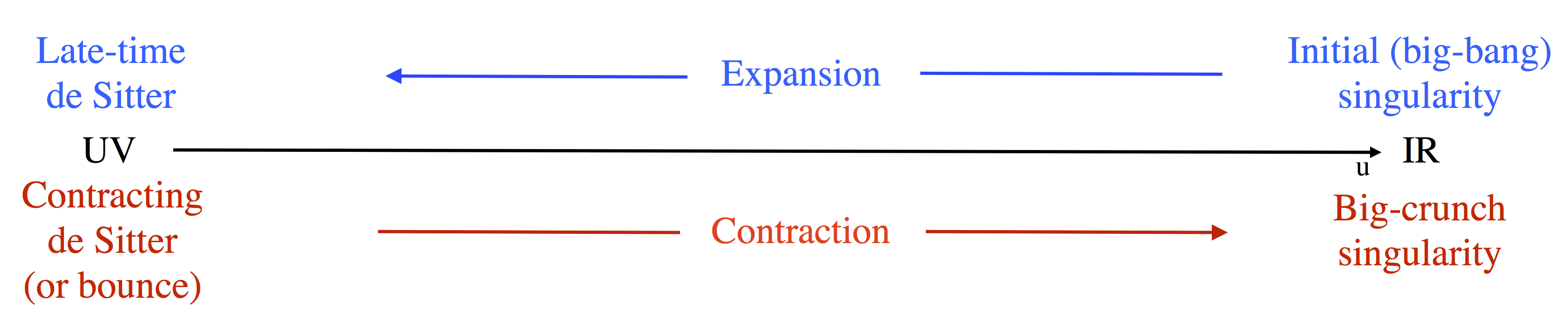
Figure 1: Mirage cosmological evolution on the brane. The black line denotes the bulk radial direction $u$, from the AdS boundary (UV) to the deep interior (IR). The upper blue line and lower red line indicate the two possible directions of the probe brane motion along the radial direction, and correspond to an expanding and contracting universe, respectively. The deep IR is perceived on the brane as a big bang or big crunch singularity, regardless of the nature of the bulk interior (IR singularity or Poincaré horizon).

The details of the cosmological history depends of course on the features of the bulk geometry and the initial conditions. However, using the above building blocks, we can sketch a few general possible histories which can emerge, independently of many of these details. In doing this, we have to remember that we have neglected the effect of brane matter (as well as bulk backreaction). At some point along the evolution of the brane-universe the brane energy densities must dominate, if we want to describe a universe close to our own. In the “normal” phase of cosmology, four-dimensional matter accurately accounts for observation. We have also assumed that the bulk dual QFT is living on Minkowski space. Other options, [16], change the brane-world cosmology.

Therefore, we may use five-dimensional effects for triggering “exotic” behavior, but we have to make sure there is room for normal textbook brane-energy driven FRW evolution along the way.

From an IR Big Bang to a UV de Sitter.

The simplest possible probe brane history is one which starts in a big bang in the IR, with the brane emerging from the IR fixed-point or singularity, reaches the UV near-boundary region, and there it undergoes a late de Sitter expansion. Note, that if there is an IR standard fixed-point, and the geometry there is that of AdS, then the big-bang singularity on the brane is an “apparent singularity”. The singularity is due to the embedding and the fact that there is a Poincaré horizon at that point in the bulk. Such brane singularities were analyzed in [42], [17] and found to be coordinate/embedding singularities.

The later de Sitter phase may look appealing at first sight for realising either an early-time inflationary phase (which would erase all memory of the IR big bang) or late-time acceleration after an intermediate cosmological phase driven by brane matter. However this picture is too simplistic, as we discuss below.

First, one may be tempted to identify the asymptotic UV de Sitter phase with the current late-time accelerating phase. Recall that the induced de Sitter scale $H_{dS}$ is, by equation (4.19)

$$H_{eff}^{2}\sim\Lambda_{eff},$$ (5.1)

where $\Lambda_{eff}$ is set by the values of the brane cosmological constant and induced Planck scale in the UV as can be seen in equation (4.18).

Naively one may think that the brane cosmological constant is set by the brane vacuum energy $\Lambda^{4}$ (including the SM loop contributions), in which case the value of $\Lambda_{eff}$ would simply be $\Lambda^{4}/M_{4}^{2}$, and we would get the old cosmological constant problem back. However, things may be subtler. First, it is not obvious what the value of the brane cosmological term $W_{B}$ should be in the far UV, because this crucially depends on how the dilaton couples to the brane fields. Second, the brane-world description is supposed to be valid only up to a UV cut-off, the scale of the messengers, coupling the standard model fields to the strongly interacting holographic sector [6]. What happens in the far UV beyond this scale requires integrating back the messengers and understanding the full dynamics. Without further investigation, what can be said here is that the description of the self-tuning mechanism studied in [6] will not be applicable, and whether the far UV mirage cosmology is compatible with the observed late-time acceleration depends on a deeper understanding of the UV of the theory.

Another possibility is that the de Sitter phase approached close to the UV fixed point may represent early universe inflation, which should be followed by reheating and radiation/matter domination. However this cannot work in the simple “vanilla” picture described in this paragraph. In fact, the more the brane approaches the UV the more the cosmology approaches de Sitter, and there is no mechanism to make de Sitter cosmological constant decay and produce Standard Model particles: there is no inflaton which can leave the slow-roll regime in this picture. A way to realise inflation in a slightly more complicated setup is discussed next.

Intermediate inflationary epoch.

A different scenario, which can give rise to a period of inflation in the middle of the bulk, is one in which the background RG flow geometry approaches an extremum of the potential from the IR, misses it and continues towards another, further extremum in the ultimate UV.

This situation can be realised in a multi-field setup, in which an extremum of the potential is attractive in some directions but repulsive in others [38]. In this case, if the background flow starts close to the attractive direction, it will spend a long time close to the fixed point (and give rise to an induced dS brane geometry) but eventually deviate away along the repulsive direction, which will effectively put an end to inflation. This can happen automatically, without fine-tuning, near a potential extremum that just violates the BF bound, [41].

There is also the possibility of realising this scenario in a single-field flow, in which the potential has multiple extrema along the $\phi$ direction, as in [37]. In such a case, the flow can approach from the IR a minimum of the bulk potential but continue on to a maximum further away. In the region close to the minimum the geometry will be approximately AdS, and the solution will be similar, for a period of time, to the one described in section 4.1.1 (since the minimum will be seen as a UV quasi-fixed point).

In order to have a long enough inflation, the solution must linger around the skipped fixed point (with the scalar field approximately constant) long enough. When the brane leaves the vicinity of the intermediate fixed point, inflation ends.

Back to self-tuning.

In order to obtain a realistic scenario, after a period of inflation (which may be realised as sketched above), one must be able to produce matter on the brane, and end up in an ordinary cosmology. For example, after the intermediate period of inflation, the brane may get caught in a self-tuning minimum and start oscillating, producing matter. If the effective potential around the minimum is steep enough, in a regime where the quasi-localised gravity is 4d, the subsequent evolution will be driven by brane-matter in an essentially four-dimensional way, as previous experience with these models suggests [24].

Deviations from standard 4d gravity may also give interesting effects in this regime. As one can show in simple models, corrections to the Friedman equation arising from the higher-dimensional nature of the setup may produce a “geometric” late-time acceleration driven by ordinary matter [27, 43].

To realise this scenario however one must go beyond the setup presented in this work. For one, brane matter and its couplings to the holographic CFT sector have to be explicitly included. Also, in order to be trapped around the self-tuning solution, a mechanism to dissipate the brane kinetic energy must be in place. This could result from energy transfer from the brane to ordinary matter or some other sector (e.g. production of light particles such as axions). In the simple setup we have been studying so far (probe limit), on the other hand, the brane energy is conserved. Even if a self-tuning solution is present, the brane will typically overshoot it, (unless its initial energy is very close to the energy corresponding to the bottom of the effective potential). The question of how a self-tuning solution may be reached starting from a non-equilibrium initial condition will be the subject of future work.

Bouncing universe.

In the absence of a mechanism to dissipate energy and be trapped in a self-tuning extremum of the effective potential, the brane will continue towards the UV of the geometry. There are two possible outcomes for the cosmological history. One, which was discussed at the beginning of this section, is that the brane continues indefinitely towards the ultimate UV and is trapped in a de Sitter phase forever. The alternative is that the UV is actually not accessible due to the features of the brane potentials: recall from section 4.1 that, in order for the probe brane equations to have a solution in the asymptotic UV, the brane potentials must be such that $W_{B}/U_{B}>0$ in the far UV. If this is not the case, the UV belongs to a “forbidden region”, (the relativistic analog of having $E<V$ in classical mechanics) and the trajectory turns around at a finite location $u_{b}$ where $\dot{u}=0$.

From the point of view of the one-dimensional problem, the UV is hidden behind a potential barrier. If this is the case, the cosmology undergoes a bounce, changes from expanding to contracting, and the brane goes back towards the IR eventually ending in a big crunch singularity. Whether the cosmology is bouncing or not may depend not only on the geometry and on the brane potentials, but also on the initial conditions, i.e the initial value of the energy, since the barrier in the UV may not be infinite and it may be overcome if the energy is large enough. More specifically, a bounce occurs whenever the variable $y$ in equation (3.14) crosses unity.

To summarise, we sketch some of the possible brane histories which may arise in this scenario:

1. Big bang $\longrightarrow$ de Sitter.

2. Big bang $\longrightarrow$ bounce $\longrightarrow$ big crunch.

3. Big bang $\longrightarrow$ Inflation period $\longrightarrow$ matter production and oscillations around a self-tuning extremum (if a suitable mechanism for dissipating energy is at work).

Appendix

Appendix A Einstein equations and junction conditions in various coordinates

In this appendix we provide the non-linear bulk equations and junction conditions for a set of useful coordinates to solve the time dependent cosmological problem.

A.1 The general diagonal ansatz

In this subsection we introduce the following ansatz for the metric:

$$ds^{2}=b(t,z)^{2}dz^{2}-n(t,z)^{2}dt^{2}+a(t,z)\delta_{ij}dx^{i}dx^{j}$$ (A.1)

where now $t$ is the time coordinate, $z$ the radial coordinate, and $x^{i}$ are three dimensional space-like coordinates. The bulk equations of motion for the metric and the scalar field are (using the convention $d_{t}=\dot{}$ and $d_{z}={}^{\prime}$ ):

$$\frac{1}{3}\Big{(}\Big{(}\frac{\dot{\varphi}}{2}\frac{b}{n}\Big{)}^{2}+\Big{(}\frac{\varphi^{\prime}}{2}\Big{)}^{2}-\frac{V(\varphi)b^{2}}{4}\Big{)}+\frac{a^{\prime}}{a}\Big{(}\frac{a^{\prime}}{a}+\frac{n^{\prime}}{n}\Big{)}-\frac{b^{2}}{n^{2}}\Big{(}\frac{\dot{a}}{a}\Big{(}\frac{\dot{a}}{a}-\frac{\dot{n}}{n}\Big{)}+\frac{\ddot{a}}{a}\Big{)} =0$$ (A.2)

$$\frac{1}{3}\Big{(}\Big{(}\frac{\varphi^{\prime}}{2}\frac{n}{b}\Big{)}^{2}+\Big{(}\frac{\dot{\varphi}}{2}\Big{)}^{2}+\frac{V(\varphi)n^{2}}{4}\Big{)}+\frac{\dot{a}}{a}\Big{(}\frac{\dot{a}}{a}+\frac{\dot{b}}{b}\Big{)}-\frac{n^{2}}{b^{2}}\Big{(}\frac{a^{\prime}}{a}\Big{(}\frac{a^{\prime}}{a}-\frac{b^{\prime}}{b}\Big{)}+\frac{a^{\prime\prime}}{a}\Big{)} =0$$

$$\frac{n^{\prime}}{n}\frac{\dot{a}}{a}+\frac{a^{\prime}}{a}\frac{\dot{b}}{b}+\frac{1}{6}\varphi^{\prime}\dot{\varphi}-\frac{\dot{a^{\prime}}}{a} =0$$

$$\Big{(}\frac{a\dot{\varphi}}{2n}\Big{)}^{2}-\Big{(}\frac{a\varphi^{\prime}}{2b}\Big{)}^{2}-\frac{1}{4}a^{2}V(\varphi)-2\frac{a}{b}\Big{(}\frac{a^{\prime}}{b}\frac{b^{\prime}}{b}-\frac{a^{\prime}}{b}\frac{n^{\prime}}{n}-\frac{a^{\prime\prime}}{b}+\frac{1}{2}\frac{a}{b}\Big{(}\frac{b^{\prime}}{b}\frac{n^{\prime}}{n}-\frac{n^{\prime\prime}}{n}\Big{)}\Big{)} ~{}+$$

$$+2\frac{a}{n}\Big{(}\frac{\dot{a}}{n}\frac{\dot{n}}{n}-\frac{\dot{a}}{n}\frac{\dot{b}}{b}-\frac{\ddot{a}}{n}+\frac{1}{2}\frac{a}{n}\Big{(}\frac{\dot{b}}{b}\frac{\dot{n}}{n}-\frac{\ddot{b}}{b}\Big{)}\Big{)}+\Big{(}\frac{a^{\prime}}{b}\Big{)}^{2}-\Big{(}\frac{\dot{a}}{n}\Big{)}^{2} =0$$

The normal vector to the brane is:

$$n_{a}=\frac{nb}{\sqrt{n^{2}-\dot{z}_{0}^{2}b^{2}}}(1,-\dot{z}_{0},0,0,0)$$ (A.3)

The non vanishing components of the brane extrinsic curvature are

$$K_{zz}=\frac{\dot{z}_{0}^{2}b^{3}}{n}X,\quad K_{zt}=-\dot{z}_{0}bnX,\quad K_{tt}=\frac{n^{3}}{b}X,\quad K_{ij}=\frac{a(n^{2}a^{\prime}+\dot{z}_{0}b^{2}\dot{a})}{bn\sqrt{n^{2}-b^{2}\dot{z}_{0}^{2}}}\delta_{ij}$$ (A.4)

with

$$X=\frac{\dot{z}_{0}^{3}b^{3}\dot{b}-n^{3}n^{\prime}-\dot{z}_{0}bn^{2}(\dot{z}_{0}b^{\prime}+2\dot{b})+b^{2}n(\dot{z}_{0}(2\dot{z}_{0}n^{\prime}+\dot{n})-\ddot{z}_{0}n)}{(n^{2}-\dot{z}_{0}^{2}b^{2})^{5/2}}$$ (A.5)

The pullback metric is given by

$$ds^{2}=-\Big{(}\hat{n}(z_{0},t)^{2}-\hat{b}(z_{0},t)^{2}\dot{r}_{0}\Big{)}dt^{2}+\hat{a}(z_{0},t)^{2}\delta_{ij}dx^{i}dx^{j}$$ (A.6)

Observe that this metric can be obtained from the original one from the equation

$$\hat{g}_{\mu\nu}=M^{a}_{\mu}M^{b}_{\nu}g_{ab}$$ (A.7)

where

$$M=\left(\begin{array}[]{ccccc}\dot{z}_{0}&1&0&0&0\\ 0&0&1&0&0\\ 0&0&0&1&0\\ 0&0&0&0&1\\ \end{array}\right)$$ (A.8)

The non vanishing components of $K_{\mu\nu}$ are

$$K_{tt}=\frac{\dot{z}_{0}^{3}b^{3}\dot{b}-n^{3}n^{\prime}-\dot{z}_{0}bn^{2}(\dot{z}_{0}b^{\prime}+2\dot{b})+b^{2}n(\dot{z}_{0}(2\dot{z}_{0}n^{\prime}+\dot{n})-\ddot{z}_{0}n)}{bn\sqrt{n^{2}-\dot{z}_{0}^{2}b^{2}}},\quad K_{ij}=\frac{a(n^{2}a^{\prime}+\dot{z}_{0}b^{2}\dot{a})}{bn\sqrt{n^{2}-b^{2}\dot{z}_{0}^{2}}}\delta_{ij}$$ (A.9)

One can verify that

$$K= K_{ab}g^{ab}=K_{\mu\nu}\hat{g}^{\mu\nu}=$$ (A.10)

$$= \frac{3(n^{2}\!\!-\!\!\dot{z}_{0}^{2}b^{2})(\dot{z}_{0}\dot{a}b^{2}+a^{\prime}n^{2})+a(\dot{z}_{0}bn^{2}(\dot{z}_{0}b^{\prime}+2\dot{b})\!\!-\!\!\dot{z}_{0}^{3}b^{3}\dot{b}+b^{2}n(\ddot{z}_{0}n\!\!-\!\!\dot{z}_{0}(2\dot{z}_{0}n^{\prime}+\dot{n}))+n^{\prime}n^{3})}{abn(n^{2}-\dot{z}_{0}^{2}b^{2})^{3/2}}$$

The non-vanishing components of $G_{\mu\nu}$ are

$$G_{tt}=\frac{3\dot{a}^{2}}{a^{2}}\quad G_{ij}=\Big{(}\frac{\dot{a}^{2}+2a\ddot{a}}{\dot{z}_{0}^{2}b^{2}-n^{2}}-\frac{\dot{a}(\dot{z}_{0}b(\dot{z}_{0}\dot{b}+\ddot{z}_{0}b)-n\dot{n}))}{(\dot{z}_{0}^{2}b^{2}-n^{2})^{2}}\Big{)}\delta_{ij}$$ (A.11)

The conditions given by the discontinuity of the extrinsic curvature and normal derivative of $\varphi$ are

$$\Big{[}K_{\tau\tau}-\hat{g}_{\tau\tau}K\Big{]}_{UV}^{IR}=\Big{[}\frac{3b\dot{r}_{0}\sqrt{n^{2}-\dot{z}_{0}^{2}b^{2}}(\dot{z}_{0}\dot{a}+a^{\prime})}{an}\Big{]}_{UV}^{IR}=$$ (A.12)

$$\Big{(}\frac{3\dot{a}\dot{\varphi}}{a}\big{(}d_{\varphi}U_{B}+\frac{\dot{a}}{a}U_{B}\big{)}+\frac{1}{2}(b^{2}\dot{z}_{0}^{2}-n^{2})W_{B}-\frac{1}{2}\dot{\varphi}^{2}Z_{B}\Big{)}_{\varphi_{0}(x)}$$

$$\Big{[}K_{ij}-\hat{g}_{ij}K\Big{]}_{UV}^{IR}=\Big{[}\frac{a(a(b^{\prime}+\dot{b}\dot{z}_{0})(b^{2}\dot{z}_{0}^{2}-2n^{2})+abn(n^{\prime}+\dot{n}\dot{z}_{0}-n\ddot{z}_{0}))}{n(n^{2}-b^{2}\dot{z}_{0}^{2})^{\frac{3}{2}}}$$ (A.13)

$$+\frac{2ab(b^{2}z_{0}^{2}-n^{2})(a^{\prime}+\dot{a}\dot{z}_{0}))}{n(n^{2}-b^{2}\dot{z}_{0}^{2})^{\frac{3}{2}}}\Big{]}_{UV}^{IR}=\Big{(}\Big{(}\frac{2a\dot{a}(n\dot{n}-b\dot{z}_{0}(\dot{b}\dot{z}_{0}+b\ddot{z}_{0}))}{(n^{2}-\dot{z}_{0}^{2}b^{2})^{2}}-\frac{2a\ddot{a}+\dot{a}^{2}}{n^{2}-\dot{z}_{0}^{2}b^{2}}\Big{)}U_{B}$$

$$+\Big{(}\frac{a^{2}\dot{\varphi}(n\dot{n}-b\dot{z}_{0}(\dot{b}\dot{z}_{0}+b\ddot{z}_{0}))}{(n^{2}-\dot{z}_{0}^{2}b^{2})^{2}}-\frac{a(2\dot{a}\dot{\varphi}+a\ddot{\varphi})}{n^{2}-\dot{z}_{0}^{2}b^{2}}\Big{)}d_{\varphi}U_{B}-\frac{a^{2}\dot{\varphi}^{2}d^{2}_{\varphi}U_{B}}{n^{2}-\dot{z}_{0}^{2}b^{2}}-\frac{a^{2}\dot{\varphi}^{2}Z_{B}}{2(n^{2}-\dot{z}_{0}^{2}b^{2})}+\frac{a^{2}W_{B}}{2}\Big{)}_{\varphi_{0}(x)}$$

$$\Big{[}n^{a}d_{a}\varphi\Big{]}_{UV}^{IR}=\Big{[}\frac{\dot{z}_{0}b^{2}\dot{\varphi}+n^{2}\varphi^{\prime}}{bn\sqrt{n^{2}-\dot{z}_{0}b^{2}}}\Big{]}_{UV}^{IR}=\Big{(}\frac{6\big{(}\frac{\dot{a}(n\dot{n}-b\dot{z}_{0}(\dot{b}\dot{z}_{0}+b\ddot{z}_{0}))}{n^{2}-b^{2}\dot{z}_{0}^{2}}-\frac{a\ddot{a}+\dot{a}^{2}}{a}\big{)}}{a(n^{2}-b^{2}\dot{z}_{0}^{2})}d_{\varphi}U_{B}+d_{\varphi}W_{B}+$$ (A.14)

$$+\Big{(}\frac{\dot{\varphi}(2(b\dot{z}_{0}(\dot{b}\dot{z}_{0}+b\ddot{z}_{0})-n\dot{n})-3a\dot{a})}{(n^{2}-b^{2}\dot{z}_{0}^{2})^{2}}+\frac{3\dot{a}\dot{\varphi}+a\ddot{\varphi}}{a(n^{2}-b^{2}\dot{z}_{0}^{2})}\Big{)}Z_{B}+\frac{\dot{\varphi}^{2}}{2n^{2}-2b^{2}\dot{z}_{0}^{2}}d_{\varphi}Z_{B}\Big{)}_{\varphi_{0}(x)}$$

A.2 The Kähler ansatz

We start with the Kähler ansatz for the metric:

$$ds^{2}=\omega(\rho,\tau)^{2}(d\rho^{2}-d\tau^{2})+\gamma(\rho,\tau)^{2}\delta_{ij}dx^{i}dx^{j}$$ (A.15)

where $\tau$ is the time coordinate, $\rho$ the radius coordinate, and $x^{i}$ are three dimensional space-like coordinates. The equations of motion for the metric and the scalar field are:

$$\frac{1}{4}\big{(}\dot{\varphi}^{2}+\varphi^{\prime 2}-V(\varphi)\omega^{2}\big{)}-\frac{3\dot{\gamma}^{2}}{\gamma^{2}}+\frac{3\dot{\gamma}\dot{\omega}}{\gamma\omega}-\frac{3\ddot{\gamma}}{\gamma}+\frac{3\gamma^{\prime 2}}{\gamma^{2}}+\frac{3\gamma^{\prime}\omega^{\prime}}{\gamma\omega} =0$$ (A.16)

$$\frac{3\dot{\omega}\gamma^{\prime}}{\gamma\omega}+\frac{1}{2}\dot{\varphi}\varphi^{\prime}+\frac{3\dot{\gamma}\omega^{\prime}}{\gamma\omega}-\frac{3\dot{\gamma}^{\prime}}{\gamma} =0$$

$$\frac{1}{4}\big{(}\dot{\varphi}^{2}+\varphi^{\prime 2}+V(\varphi)\omega^{2}\big{)}+\frac{3\dot{\gamma}^{2}}{\gamma^{2}}+\frac{3\dot{\gamma}\dot{\omega}}{\gamma\omega}-\frac{3\gamma^{\prime 2}}{\gamma^{2}}+\frac{3\gamma^{\prime}\omega^{\prime}}{\gamma\omega}-\frac{3\gamma^{\prime\prime}}{\gamma} =0$$

$$\frac{\gamma^{2}}{4\omega^{2}}\Big{(}(\dot{\varphi}^{2}-\varphi^{\prime 2}-V(\varphi){\omega^{2}}\Big{)}-\frac{\dot{\gamma}^{2}}{\omega^{2}}+\frac{\gamma^{2}\dot{\omega}^{2}}{\omega^{4}}-\frac{2\gamma\ddot{\gamma}}{\omega^{2}}-\frac{\gamma^{2}\ddot{\omega}}{\omega^{3}} +~{}~{}~{}$$

$$+\frac{\gamma^{\prime 2}}{\omega^{2}}-\frac{\gamma^{2}\omega^{\prime 2}}{\omega^{4}}+\frac{2\gamma\gamma^{\prime\prime}}{\omega^{2}}+\frac{\gamma^{2}\omega^{\prime\prime}}{\omega^{3}} =0$$

The normal vector to the brane is:

$$n_{a}=\frac{\omega}{\sqrt{(1-\dot{\rho}_{0}^{2})}}(1,-\dot{\rho}_{0},0,0,0)$$ (A.17)

The non vanishing components of the brane extrinsic curvature are:

$$K_{ab}=\nabla_{a}n_{b}-n^{c}n_{a}\nabla_{c}n_{b}=\frac{1}{2}(\nabla_{a}n_{b}+\nabla_{b}n_{a}-n^{c}\nabla_{c}(n_{a}n_{b}))$$ (A.18)

with:

$$K_{\rho\rho}=-\dot{\rho}_{0}^{2}X,\quad K_{\rho\tau}=\dot{\rho}_{0}X,\quad K_{\tau\tau}=-X,\quad K_{ij}=\frac{\gamma(\dot{\gamma}\dot{\rho}_{0}+\gamma^{\prime})}{\omega\sqrt{1-\dot{\rho}_{0}^{2}}}\delta_{ij}$$ (A.19)

where

$$X=\frac{(1-\dot{\rho}_{0}^{2})(\dot{\omega}\dot{\rho}_{0}+\omega^{\prime})+\omega\ddot{\rho}_{0}}{(1-\dot{\rho}_{0}^{2})\sqrt{1-\dot{\rho}_{0}^{2}}},$$ (A.20)

The induced metric $\hat{g}_{\mu\nu}$ is given by

$$ds^{2}=-\Big{(}\hat{\omega}(\rho_{0}(\tau),\tau)^{2}-\dot{\rho}_{0}(\tau)\Big{)}d\tau^{2}+\hat{\gamma}(\rho_{0}(\tau),\tau)^{2}\delta_{ij}dx^{i}dx^{j}$$ (A.21)

Observe that the brane induced metric can be obtained from the bulk metric using the matrix $M$ as in the equation

$$\hat{g}_{\mu\nu}=M_{\mu}^{a}M_{\nu}^{b}g_{ab}$$ (A.22)

where

$$M=\left(\begin{array}[]{ccccc}\dot{\rho}_{0}(\tau)&1&0&0&0\\ 0&0&1&0&0\\ 0&0&0&1&0\\ 0&0&0&0&1\\ \end{array}\right)$$ (A.23)

The non vanishing components of $K_{\mu\nu}$ are

$$K_{tt}=\frac{(\dot{\rho}_{0}-1)(\dot{\omega}\dot{\rho}_{0}+\omega^{\prime})-\omega\ddot{\rho}_{0}}{\sqrt{1-\dot{\rho}_{0}^{2}}},\quad K_{ij}=\frac{\gamma(\dot{\gamma}\dot{\rho}_{0}+\gamma^{\prime})}{\omega\sqrt{1-\dot{\rho}_{0}^{2}}}\delta_{ij}$$ (A.24)

One can verify that

$$K=K_{ab}g^{ab}=K_{\mu\nu}\hat{g}^{\mu\nu}=-\frac{3\omega(\dot{\rho}_{0}^{2}-1)(\dot{\gamma}\dot{\rho}_{0}+\gamma^{\prime})+\gamma((\dot{\rho}_{0}^{2}-1)(\dot{\omega}\dot{\rho}_{0}+\omega^{\prime})-\omega\ddot{\rho}_{0})}{\gamma\omega^{2}(1-\dot{\rho}_{0}^{2})^{3/2}}$$ (A.25)

The non-vanishing components of the Einstein tensor $G_{\mu\nu}$ are

$$G_{\tau\tau}=\frac{3\dot{\gamma}^{2}}{\gamma^{2}},\quad G_{ij}=\Big{(}\frac{\dot{\gamma}^{2}}{\omega^{2}}+\frac{2\gamma(\ddot{\gamma}\omega-\dot{\gamma}\dot{\omega})}{\omega^{3}}-\frac{2\gamma\dot{\gamma}}{\omega^{2}}\frac{\dot{\rho}_{0}\ddot{\rho}_{0}}{(\dot{\rho}_{0}^{2}-1)^{2}}\Big{)}\delta_{ij}$$ (A.26)

The conditions given by the discontinuity of the extrinsic curvature and normal derivative of $\varphi$ are

$$\Big{[}K_{\tau\tau}-\hat{g}_{\tau\tau}K\Big{]}_{UV}^{IR}=\Big{[}\frac{3\omega}{\gamma}(\dot{\rho}\dot{\gamma}+\gamma^{\prime})\sqrt{1-\dot{\rho}_{0}^{2}}\Big{]}_{UV}^{IR}=$$ (A.27)

$$=\big{(}\frac{\gamma^{2}(\omega^{2}W_{B}(\dot{\rho}_{0}^{2}-1)-\dot{\varphi}^{2}Z_{B})+6\gamma\dot{\gamma}\dot{\varphi}d_{\varphi}U_{B}+6\dot{\gamma}^{2}U_{B}}{2\gamma^{2}}\Big{)}_{\varphi_{0}(x)}$$

$$\Big{[}K_{ij}-\hat{g}_{ij}K\Big{]}_{UV}^{IR}=\Big{[}-\frac{\gamma(\gamma(\ddot{\rho}_{0}\omega-(\dot{\rho}_{0}^{2}-1)(\dot{\rho}_{0}\dot{\omega}+\omega^{\prime}))-2(\dot{\rho}_{0}^{2}-1)\omega(\dot{\rho}_{0}\dot{\gamma}+\gamma^{\prime}))}{(1-\dot{\rho}_{0}^{2})^{3/2}\omega^{2}}\delta_{ij}\Big{]}_{UV}^{IR}$$ (A.28)

$$=\Big{(}-\Big{(}\frac{2\gamma(\omega\ddot{\gamma}-\dot{\gamma}\dot{\omega})+\omega\dot{\gamma}^{2}}{\omega^{3}(1-\dot{\rho}_{0}^{2})}\frac{2\gamma\dot{\gamma}\dot{\rho}_{0}\ddot{\rho}_{0}}{\omega^{2}(1-\dot{\rho}_{0}^{2})^{2}}\Big{)}U_{B}-\Big{(}\frac{\gamma(\dot{\varphi}(2\omega\dot{\gamma}-\gamma\dot{\omega})+\gamma\omega\ddot{\varphi})}{\omega^{3}(1-\dot{\rho}_{0}^{2})}+$$

$$+\frac{\gamma^{2}\dot{\rho}_{0}\ddot{\rho}_{0}\dot{\varphi}}{\omega^{2}(1-\dot{\rho}_{0}^{2})^{2}}\Big{)}d_{\varphi}U_{B}-\frac{\gamma^{2}\dot{\varphi}^{2}}{\omega^{2}(1-\dot{\rho}_{0}^{2})}d_{\varphi}^{2}U_{B}+\frac{\gamma^{2}}{2}W_{B}-\frac{\gamma^{2}\dot{\varphi}^{2}}{2\omega^{2}(1-\dot{\rho}_{0}^{2})}Z_{B}\Big{)}_{\varphi_{0}(x)}$$

$$\Big{[}n^{a}d_{a}\varphi\Big{]}_{UV}^{IR}=\Big{[}\frac{\varphi^{\prime}+\dot{\rho}_{0}\dot{\varphi}}{\omega\sqrt{1-\dot{\rho}_{0}^{2}}}\Big{]}_{UV}^{IR}=\Big{(}6\Big{(}\frac{\gamma\omega\ddot{\gamma}-\gamma\dot{\gamma}\dot{\omega}+\omega\dot{\gamma}^{2}}{\gamma^{2}\omega^{3}(\dot{\rho}_{0}^{2}-1)}-\frac{\dot{\gamma}\dot{\rho}_{0}\ddot{\rho}_{0}}{\gamma\omega^{2}(\dot{\rho}_{0}^{2}-1)^{2}}\Big{)}d_{\varphi}U_{B}+$$ (A.29)

$$+d_{\varphi}W_{B}+\Big{(}\frac{\dot{\varphi}(2\gamma\omega^{2}\dot{\rho}_{0}\ddot{\rho}_{0}-3\gamma^{2}\dot{\gamma})}{\gamma\omega^{4}(1-\dot{\rho}_{0}^{2})^{2}}+\frac{\dot{\varphi}(3\omega\dot{\gamma}-2\gamma\dot{\omega})+\gamma\omega\ddot{\varphi}}{\gamma\omega^{3}(1-\dot{\rho}_{0}^{2})}\Big{)}Z_{B}-\frac{\dot{\varphi}^{2}}{2\omega^{2}(1-\dot{\rho}_{0}^{2})}d_{\varphi}Z_{B}\Big{)}_{\varphi_{0}(x)}$$

Observe that in these equations the time derivative on the RHS is a total derivative $\frac{d}{d\tau}=\dot{}$, and the functions $\gamma$, $\omega$ and $\varphi$ depend on $(\rho,\tau)$ on the LHS and on $(\rho_{0}(\tau),\tau)$ on the RHS. In other words, on the LHS we have the 5d objects while on the RHS we have the 4d ones.

A.3 The Chesler-Yaffe ansatz

In this appendix we introduce the Chesler-Yaffe ansatz for the metric:

$$ds^{2}=-\frac{2}{z^{2}}dvdz-{\bf A}dv^{2}+{\bf{\bf\Sigma}}^{2}\delta_{ij}dx^{i}dx^{j}$$ (A.30)

with $x^{i}$ the three dimensional space like coordinates, and $z$ and $v$ time-like coordinates. The bulk equations of motion for metric and scalar field are:

$$-3\frac{{\bf\Sigma^{\prime\prime}}}{{\bf\Sigma}}-\frac{6}{z}\frac{\bf\Sigma^{\prime}}{{\bf\Sigma}}+\frac{1}{2}\varphi^{\prime 2} = 0$$ (A.31)

$$\frac{V(\varphi)}{4z^{2}}-\frac{6z{\bf A}{\bf\Sigma^{\prime}}}{\bf{\Sigma}}-\frac{3z^{2}{\bf A^{\prime}}{\bf\Sigma^{\prime}}}{2{\bf\Sigma}}-\frac{3z^{2}{\bf A}{\bf\Sigma^{\prime 2}}}{\bf\Sigma^{2}}+\frac{1}{4}z^{2}{\bf A}\varphi^{\prime 2}-\frac{3z^{2}{\bf A}{\bf\Sigma^{\prime\prime}}}{\bf\Sigma}+\frac{6{\bf\Sigma^{\prime}}{\bf\dot{\Sigma}}}{\bf\Sigma^{2}}+\frac{3{\bf\dot{\Sigma}^{\prime}}}{\bf\Sigma} = 0$$

$$\frac{1}{4}{\bf A}V(\varphi)-\frac{6z^{3}{\bf A^{2}}{\bf\Sigma^{\prime}}}{\bf\Sigma}-\frac{3z^{4}{\bf AA^{\prime}\Sigma^{\prime}}}{2{\bf\Sigma}}-\frac{3z^{4}{\bf A^{2}\Sigma^{\prime 2}}}{2{\bf\Sigma^{2}}}+\frac{1}{4}z^{4}{\bf A}\varphi^{\prime 2}-\frac{3z^{4}{\bf A^{2}\Sigma^{\prime\prime}}}{\bf\Sigma} ~{}+$$

$$+\frac{3z^{2}{\bf\Sigma^{\prime}\dot{A}}}{2{\bf\Sigma}}-\frac{3z^{2}{\bf A^{\prime}\dot{\Sigma}}}{2{\bf\Sigma}}+\frac{6z^{2}{\bf A\Sigma^{\prime}\dot{\Sigma}}}{\bf\Sigma^{2}}-\frac{1}{2}z^{2}{\bf A}\varphi^{\prime}\dot{\varphi}+\frac{1}{2}\dot{\varphi}^{2}+\frac{6z^{2}{\bf A\dot{\Sigma}^{\prime}}}{\bf\Sigma}-\frac{3{\bf\ddot{\Sigma}}}{\bf\Sigma} = 0$$

$$-\frac{1}{4}V(\varphi){\bf\Sigma^{2}}+z^{3}{\bf\Sigma^{2}A^{\prime}}+4z^{3}{\bf A\Sigma\Sigma^{\prime}}+2z^{4}{\bf\Sigma A^{\prime}\Sigma^{\prime}}+z^{4}{\bf A\Sigma^{\prime 2}}-\frac{1}{4}z^{4}{\bf A\Sigma^{2}}\varphi^{\prime 2} ~{}+$$

$$+\frac{1}{2}z^{4}{\bf\Sigma^{2}A^{\prime\prime}}+2z^{4}{\bf A\Sigma\Sigma^{\prime\prime}}-2z^{2}{\bf\Sigma^{\prime}\dot{\Sigma}}+\frac{1}{2}z^{2}{\bf\Sigma^{2}}\varphi^{\prime}\dot{\varphi}-4z^{2}{\bf\Sigma\dot{\Sigma}^{\prime}} = 0$$

The normal vector to the brane is:

$$n_{a}=\frac{1}{z_{0}\sqrt{z_{0}^{2}{\bf A}+2\dot{z}_{0}}}(1,-\dot{z}_{0},0,0,0)$$ (A.32)

The pullback metric is given by

$$ds^{2}=-\Big{(}\hat{\bf A}(z_{0}(v),v)+2\frac{\dot{z}_{0}(v)}{z_{0}(v)^{2}}\Big{)}dv^{2}+\hat{\bf\Sigma}(z_{0}(v),v)dx^{i}dx^{j}\delta_{ij}$$ (A.33)

with this time the $M^{a}_{\mu}$ in (A.22) is

$$M=\left(\begin{array}[]{ccccc}\dot{z}_{0}&1&0&0&0\\ 0&0&1&0&0\\ 0&0&0&1&0\\ 0&0&0&0&1\\ \end{array}\right)$$ (A.34)

The non vanishing components of $K_{\mu\nu}$ are

$$K_{vv}=\frac{4\dot{z}_{0}^{2}-z_{0}^{3}\dot{\hat{{\bf A}}}-2z_{0}\ddot{z}_{0}}{2z_{0}^{2}\sqrt{z_{0}^{2}\hat{\bf A}+2\dot{z}_{0}}}\quad K_{ij}=-\frac{z_{0}\hat{\bf\Sigma}\dot{\hat{\bf\Sigma}}}{\sqrt{z_{0}^{2}\hat{\bf A}+2\dot{z}_{0}}}\delta_{ij}$$ (A.35)

One can verify that $K=K_{ab}g^{ab}=K_{\mu\nu}\hat{g}^{\mu\nu}$. In this case we have

$$K=-\frac{3z_{0}\dot{\hat{\bf\Sigma}}}{\hat{\bf{\Sigma}}\sqrt{z_{0}^{2}\hat{\bf A}+2\dot{z}_{0}}}-\frac{4\dot{z}_{0}^{2}+z_{0}^{3}\dot{\hat{{\bf A}}}-2z_{0}\ddot{z}_{0}}{(z_{0}^{2}\hat{\bf A}-2\dot{z}_{0})^{\frac{3}{2}}}$$ (A.36)

The matching conditions can be written as

$$\Big{[}K_{\tau\tau}-\hat{g}_{\tau\tau}K\Big{]}_{UV}^{IR}=\Big{[}\frac{3\sqrt{z_{0}^{2}\hat{\bf A}+2\dot{z}_{0}}(\dot{z}_{0}\hat{\bf\Sigma}^{\prime}-\dot{\hat{\bf\Sigma}})}{z_{0}\hat{\bf\Sigma}}\Big{]}_{UV}^{IR}=$$ (A.37)

$$\Big{(}\frac{3{\bf\dot{\hat{\bf\Sigma}}^{2}}}{{\hat{\bf\Sigma}}^{2}}U_{B}+\frac{3{\bf\dot{\hat{\bf\Sigma}}}\dot{\varphi}}{\hat{\bf\Sigma}}d_{\varphi}U_{B}-\frac{1}{2}{\hat{\bf A}}W_{B}-\frac{\dot{z}_{0}}{z_{0}^{2}}W_{B}-\frac{1}{2}\dot{\varphi}^{2}Z_{B}\Big{)}_{\varphi_{0}(x)}$$

$$\Big{[}K_{ij}-\hat{g}_{ij}K\Big{]}_{UV}^{IR}=\Big{[}-\frac{2z_{0}\hat{\bf\Sigma}(\dot{z}_{0}\hat{\bf\Sigma}^{\prime}-\dot{\hat{\bf\Sigma}})}{\sqrt{z_{0}^{2}\hat{\bf A}+2\dot{z}_{0}}}+\frac{\hat{\bf\Sigma}^{2}(4\dot{z}_{0}^{2}-z_{0}^{3}\dot{\hat{{\bf A}}}-2z_{0}\ddot{z}_{0})}{(z_{0}^{2}\hat{\bf A}+2\dot{z}_{0})^{\frac{3}{2}}}\Big{]}_{UV}^{IR}$$ (A.38)

$$=\Big{(}\frac{z_{0}^{2}({\hat{\bf\Sigma}}(\dot{\hat{{\bf\Sigma}}}(z_{0}^{2}\dot{\hat{{\bf A}}}+2\ddot{z}_{0})-2\ddot{\hat{{\bf\Sigma}}}(z_{0}^{2}\hat{\bf A}+2\dot{z}_{0}))-\dot{\hat{{\bf\Sigma}}}^{2}(z_{0}^{2}\hat{\bf A}+2\dot{z}_{0}))U_{B}}{(z_{0}^{2}\hat{\bf A}+2\dot{z}_{0})^{2}}+$$

$$+\frac{z_{0}^{2}\hat{\bf\Sigma}(\dot{\varphi}(\hat{\bf\Sigma}(z_{0}^{2}\dot{\hat{{\bf A}}}+2\ddot{z}_{0})-4\dot{\hat{{\bf\Sigma}}}(z_{0}^{2}\hat{\bf A}+2\dot{z}_{0}))-2\hat{\bf\Sigma}\ddot{\varphi}(z_{0}^{2}\hat{\bf A}+2\dot{z}_{0}))d_{\varphi}U_{B}}{2(z_{0}^{2}\hat{\bf A}+2\dot{z}_{0})^{2}}-$$

$$-\frac{z_{0}^{2}\hat{\bf\Sigma}^{2}\dot{\varphi}^{2}d_{\varphi}^{2}U_{B}}{z_{0}^{2}\hat{\bf A}+2\dot{z}_{0}}-\frac{z_{0}^{2}\hat{\bf\Sigma}^{2}\dot{\varphi}^{2}Z_{B}}{2z_{0}^{2}\hat{\bf A}+4\dot{z}_{0}}+\frac{\hat{\bf\Sigma}^{2}W_{B}}{2}\Big{)}_{\varphi_{0}(x)}$$

$$\Big{[}n^{a}d_{a}\varphi\Big{]}_{UV}^{IR}= \Big{[}\frac{z_{0}(\varphi^{\prime}(z_{0}^{2}\hat{\bf A}+z_{0}^{\prime})-\dot{\varphi})}{\sqrt{z_{0}^{2}\hat{\bf A}+2\dot{z}_{0}}}\Big{]}_{UV}^{IR}=\frac{z_{0}^{2}d_{\varphi}Z_{B}\dot{\varphi}^{2}}{2z_{0}^{2}\hat{\bf A}+4\dot{z}_{0}}+d_{\varphi}W_{B}+$$ (A.39)

$$+ \frac{3z_{0}^{2}d_{\varphi}U_{B}(\hat{\bf\Sigma}(\dot{\hat{{\bf\Sigma}}}(z_{0}^{2}\dot{\hat{{\bf A}}}+2\ddot{z}_{0})-2\ddot{\hat{{\bf\Sigma}}}(z_{0}^{2}\hat{\bf A}+2\dot{z}_{0}))-2\dot{\hat{{\bf\Sigma}}}^{2}(z_{0}^{2}\hat{\bf A}+2\dot{z}_{0}))}{\hat{\bf\Sigma}^{2}(z_{0}^{2}\hat{\bf A}+2\dot{z}_{0}^{2})}$$

$$+ \frac{z_{0}^{2}Z_{B}(\hat{\bf\Sigma}\ddot{\varphi}(z_{0}^{2}\hat{\bf A}+2\dot{z}_{0})-\dot{\varphi}(\hat{\bf\Sigma}(z^{2}\dot{\hat{{\bf A}}}+2\ddot{z}_{0})-3\dot{\hat{{\bf\Sigma}}}(z_{0}^{2}\hat{\bf A}+2\dot{z}_{0})+3z_{0}^{2}\hat{\bf\Sigma}^{2}\dot{\hat{{\bf\Sigma}}}))}{\hat{\bf\Sigma}(z_{0}^{2}\hat{\bf A}+2\dot{z}_{0}^{2})}$$

A.4 The coupled wave equation ansatz

We finally present in this appendix the coupled wave equation ansatz for the metric:

$$ds^{2}=e^{2\nu}B^{-2/3}(dr^{2}-dt^{2})+B^{2/3}\delta^{ij}dx_{i}dx_{j}$$ (A.40)

with $t$ the time coordinate, $r$ the radial coordinate, and $x^{i}$ the three dimensional space-like coordinate. In this system of coordinates, the bulk equations of motion take a simple form and they are:

$$\ddot{B}-B^{\prime\prime} = e^{2\nu}B^{\frac{1}{3}}V(\varphi)$$ (A.41)

$$\ddot{\nu}-\nu^{\prime\prime} = \frac{e^{2\nu}}{6}B^{-\frac{2}{3}}V(\varphi)-\frac{\dot{\varphi}^{2}}{4}+\frac{\varphi^{\prime 2}}{4}$$ (A.42)

$$\ddot{\varphi}-\varphi^{\prime\prime} = -e^{2\nu}B^{-\frac{2}{3}}d_{\varphi}V-\frac{\dot{B}\dot{\varphi}}{B}+\frac{B^{\prime}\varphi^{\prime}}{B}$$ (A.43)

$$\dot{\nu}B^{\prime}+\nu^{\prime}\dot{B}-\dot{B}^{\prime} = \frac{B}{2}\dot{\varphi}\varphi^{\prime}$$ (A.44)

$$2B^{\prime}\nu^{\prime}+2\dot{B}\dot{\nu}-\ddot{B}-B^{\prime\prime} = \frac{B}{2}B(\dot{\varphi}^{2}+\varphi^{\prime 2})$$ (A.45)

Note the coupled two dimensional wave form of the first three equations for each of the variables while the latter two couple the variables non-linearly. This Anzatz was first used by Taub to analyse planar symmetric metrics in vacuum [45]. The bulk equations can be further simplified upon going to light-like coordinates [31]. While the matching conditions are:

$$\Big{[}K_{tt}-\hat{g}_{tt}K\Big{]}_{UV}^{IR}=-\Big{[}\frac{e^{\hat{\nu}}}{\hat{B}^{\frac{4}{3}}}\sqrt{1-\dot{r}_{0}^{2}}(\dot{r}_{0}\dot{\hat{B}}+(1+\dot{r}_{0}^{2})\hat{B}^{\prime})\Big{]}_{UV}^{IR}=$$ (A.46)

$$\Big{(}\frac{\dot{\hat{B}}\dot{\varphi}d_{\varphi}U_{B}}{\hat{B}}+\frac{\dot{\hat{B}}^{2}U_{B}}{3\hat{B}^{2}}+\frac{e^{2\hat{\nu}}\dot{r}_{0}^{2}W_{B}}{2\hat{B}^{2/3}}-\frac{e^{2\hat{\nu}}W_{B}}{2\hat{B}^{2/3}}+\frac{Z_{B}\dot{\varphi}^{2}}{2}\Big{)}_{\varphi_{0}(x)}$$

$$\Big{[}K_{ij}-\hat{g}_{ij}K\Big{]}_{UV}^{IR}=\Big{[}\frac{(\dot{\hat{B}}+3\hat{B}\dot{\hat{\nu}})\dot{r}_{0}(1-\dot{r}_{0}^{2})+(\hat{B}^{\prime}+3\hat{B}\hat{\nu}^{\prime})(1-\dot{r}_{0}^{4})+3\hat{B}\ddot{r}_{0}}{3e^{\hat{\nu}}(1-\dot{r}_{0}^{2})^{\frac{3}{2}}}\Big{]}_{UV}^{IR}=$$ (A.47)

$$\Big{(}\frac{{\hat{B}}^{\frac{2}{3}}W_{B}}{2}-\Big{(}\frac{\hat{B}^{\frac{1}{3}}(\dot{\varphi}(\dot{\hat{B}}-\hat{B}\dot{\hat{\nu}})+\hat{B}\ddot{\varphi})}{1-\dot{r}_{0}^{2}}+\frac{\hat{B}^{\frac{4}{3}}\dot{r}_{0}\ddot{r}_{0}\dot{\varphi}}{(1-\dot{r}_{0}^{2})^{2}}\Big{)}\frac{d_{\varphi}U_{B}}{e^{2\hat{\nu}}}+\frac{\hat{B}^{\frac{4}{3}}\dot{\varphi}^{2}Z_{B}}{2e^{2\hat{\nu}}(1-\dot{r}_{0}^{2})}$$

$$-\Big{(}\frac{2\hat{B}^{\frac{1}{3}}\dot{\hat{B}}\dot{r}_{0}\ddot{r}_{0}}{3(1-\dot{r}_{0}^{2})^{2}}+\frac{6\hat{B}\ddot{\hat{B}}-6\hat{B}\dot{\hat{B}}\dot{\hat{\nu}}-\dot{\hat{B}}^{2}}{9\hat{B}^{\frac{2}{3}}(1-\dot{r}_{0}^{2})}\Big{)}\frac{U_{B}}{e^{2\hat{\nu}}}-\frac{\hat{B}^{\frac{4}{3}}\dot{\varphi}^{2}}{1-\dot{r}_{0}^{2}}\frac{d_{\varphi}^{2}U_{B}}{e^{2\hat{\nu}}}\Big{)}_{\varphi_{0}(x)}$$

$$\Big{[}n^{a}d_{a}\varphi\Big{]}_{UV}^{IR}=-\Big{[}\frac{e^{\hat{\nu}}}{\hat{B}^{\frac{1}{3}}}\frac{(1-\dot{r}_{0}^{2})\varphi^{\prime}-\dot{r}_{0}\dot{\varphi}}{\sqrt{1-\dot{r}_{0}^{2}}}\Big{]}_{UV}^{IR}=\Big{(}\Big{(}\frac{\dot{\hat{B}}\dot{\hat{\nu}}-\ddot{\hat{B}}}{1-\dot{r}_{0}^{2}}-\frac{\dot{\hat{B}}\dot{r}_{0}\ddot{r}_{0}}{(1-\dot{r}_{0}^{2})^{2}}\Big{)}\frac{2d_{\varphi}U_{B}}{e^{2\hat{\nu}}\hat{B}^{\frac{1}{3}}}+d_{\varphi}W_{B}$$ (A.48)

$$+\frac{\hat{B}^{\frac{2}{3}}\dot{\varphi}^{2}d_{\varphi}Z_{B}}{2e^{2\hat{\nu}}(1-2\dot{r}_{0}^{2})}-\Big{(}\frac{3\hat{B}\dot{\varphi}(e^{-2\hat{\nu}}{\hat{B}}^{\frac{1}{3}}\dot{\hat{B}}-2\dot{r}_{0}\ddot{r}_{0})}{(1-\dot{r}_{0}^{2})^{2}}-\frac{(5\dot{\hat{B}}-6\hat{B}\dot{\hat{\nu}})\dot{\varphi}+3\hat{B}\ddot{\varphi}}{1-\dot{r}_{0}^{2}}\Big{)}\frac{Z_{B}}{3\hat{B}^{\frac{1}{3}}e^{2\hat{\nu}}}\Big{)}_{\varphi_{0}(x)}$$

Appendix B The time-dependent domain-wall ansatz

In this appendix we make a first attempt in solving the time dependent equations for the probe limit. To do that we focus on the simple ansatz

$$ds^{2}=du^{2}+e^{2\mathcal{A}(u,t)}(-dt^{2}+\delta_{ij}dx^{i}dx^{j})$$ (B.1)

that can be seen as a simplification of the various cases analyzed in appendix A to a time dependent metric specified by a single scalar function. To simplify we first assess the existence of a solution performing a linearised analysis. This has indeed a double objective: first of all it allows us to assess if a solution in this form exists. Indeed in general, a non-linear solution will have a linear limit as well. Hence, if a linear solution is not found, we can conclude that, quite generically, also a full non-linear solution does not exist. The reverse is of course not true: i.e. a linear solution will not be in general a solution for the full non-linear system. Secondly, if a linear solution is found, this can put the basis of the quest for the full non-linear solution based on solving the equations order by order. As a result of our analysis, we show that a generic linear solution does not exist, and therefore very probably also a generic non-linear solution of the form (B.1), does not exist.

To show this we start by linearizing the metric ansatz in (B.1) as

$$ds^{2}=du^{2}+\alpha(u,t)\eta_{\mu\nu}dx^{\mu}dx^{\nu}$$ (B.2)

Denoting time-derivatives by a dot and a $u$-derivatives by a prime, the bulk equations of motion (A.2) take the form

$$-V^{\prime}-2\frac{\dot{\alpha}\dot{\varphi}}{\alpha^{3}}-\frac{\ddot{\varphi}}{\alpha^{2}}+4\frac{\alpha^{\prime}\varphi^{\prime}}{\alpha}+\varphi^{\prime\prime} = 0$$

$$4\frac{(\dot{\alpha})^{2}}{\alpha^{2}}-\frac{1}{2}(\dot{\varphi})^{2}-2\frac{\ddot{\alpha}}{\alpha} = 0$$

$$3\frac{\dot{\alpha}\alpha^{\prime}}{\alpha^{2}}-\frac{1}{2}\dot{\varphi}\varphi^{\prime}-3\frac{\dot{\alpha}^{\prime}}{\alpha} = 0$$

$$-\frac{(\dot{\alpha})^{2}}{\alpha^{4}}-\frac{\ddot{\alpha}}{\alpha^{3}}+3\frac{(\alpha^{\prime})^{2}}{\alpha^{2}}-\frac{1}{2}(\varphi^{\prime})^{2}-3\frac{\alpha^{\prime\prime}}{\alpha} = 0$$

$$V-3\frac{(\dot{\alpha})^{2}}{\alpha^{4}}-3\frac{\ddot{\alpha}}{\alpha^{3}}+9\frac{(\alpha^{\prime})^{2}}{\alpha^{2}}+3\frac{\alpha^{\prime\prime}}{\alpha} = 0$$ (B.3)

By evaluating $\alpha(u,t)$ on the brane trajectory $u=u_{0}(t)$, we can define $\hat{\alpha}(u_{0}(t),t)$. Using this notation, the matching conditions on the brane become (to simplify notation, we set, $u_{0}(t)\equiv u_{0}$)

$$[K_{tt}-\gamma_{tt}K]_{IR}^{UV}=\Big{[}\frac{3\dot{u}_{0}\sqrt{\hat{\alpha}^{2}-\dot{u}_{0}^{2}}({\hat{\alpha}}^{\prime}\dot{u}_{0}+\dot{\hat{\alpha}})}{\hat{\alpha}^{2}}\Big{]}_{IR}^{UV}$$

$$= \big{(}-\frac{1}{2}W_{B}\alpha^{2}+3U_{B}\frac{(\dot{\alpha})^{2}}{\alpha^{2}}+3U_{B}^{\prime}\frac{\dot{\alpha}\dot{\varphi}}{\alpha}-\frac{1}{2}Z_{B}(\varphi)^{2}\big{)}_{\varphi(x)}$$ (B.4)

$$[K_{ii}-\gamma_{ii}K]_{IR}^{UV}=\Big{[}\frac{-{\hat{\alpha}}^{3}\ddot{u}_{0}-{\hat{\alpha}}^{2}\dot{u}_{0}({\hat{\alpha}}^{\prime}\dot{u}_{0}+\dot{\hat{\alpha}})+2\dot{u}_{0}^{3}({\hat{\alpha}}^{\prime}\dot{u}_{0}+\dot{\hat{\alpha}})}{({\hat{\alpha}}^{2}-\dot{u}_{0}^{2})^{3/2}}\Big{]}_{IR}^{UV}$$

$$=\big{(}\frac{1}{2}W_{B}\alpha^{2}+U_{B}\frac{(\dot{\alpha})^{2}}{\alpha^{2}}-U_{B}^{\prime}\frac{\dot{\alpha}\dot{\varphi}}{\alpha}+\frac{1}{2}Z_{B}(\dot{\varphi})^{2}-U_{B}^{\prime\prime}(\dot{\varphi})^{2}-2U_{B}\frac{\ddot{\alpha}}{\alpha}-U_{B}^{\prime}\ddot{\varphi}\big{)}_{\varphi(x)}$$ (B.5)

$$[n^{a}\partial_{a}\varphi]_{IR}^{UV}=\Big{[}\frac{\varphi^{\prime}}{\sqrt{1-(\dot{u}_{0}/\alpha)^{2}}}\Big{]}_{IR}^{UV}=\big{(}W_{B}^{\prime}-2Z_{B}\frac{\dot{\alpha}\dot{\varphi}}{\alpha^{3}}+Z_{B}^{\prime}\frac{(\dot{\varphi})^{2}}{2\alpha^{2}}-6U_{B}^{\prime}\frac{\ddot{\alpha}}{\alpha^{3}}+Z_{B}\frac{\ddot{\varphi}}{\alpha^{2}}\big{)}_{\varphi(x)}$$ (B.6)

To explicitly solve the equations we need, in principle, to specify the form of the potential. Nevertheless, we observe in the following that it is not needed to specify the potential to assess the existence or not of the generic solution. Hence, in the following, we keep the potential generic, without restricting to any functional form. To proceed, expand the scalar functions $\varphi$ and $\alpha$ as:

$$\alpha(u,t)=a(u)+\phi_{1}(u,t),\quad\varphi(u,t)=\varphi_{0}(u)+\phi_{2}(u,t)$$ (B.7)

The equations of motion at zeroth order are:

$$-V^{\prime}(\varphi_{0})+\frac{4a^{\prime}}{a}\varphi_{0}^{\prime}+\varphi_{0}^{\prime\prime} = 0$$ (B.8)

$$\frac{3a^{\prime 2}}{a^{2}}-\frac{1}{2}\varphi_{0}^{\prime 2}-\frac{3a^{\prime\prime}}{a} = 0$$ (B.9)

$$V(\varphi_{0})+\frac{12a^{\prime 2}}{a^{2}}-\frac{1}{2}\varphi_{0}^{\prime 2} = 0$$ (B.10)

while at first order we obtain:

$$-\frac{\ddot{\phi}_{2}}{a^{2}}+\frac{4a^{\prime}\phi_{2}^{\prime}}{a}-\frac{4\varphi_{0}\phi_{1}a^{\prime}}{a^{2}}+\frac{4\varphi_{0}^{\prime}\phi_{1}^{\prime}}{a}-\phi_{2}V^{\prime\prime}(\varphi_{0})+\phi_{2}^{\prime\prime}=0$$ (B.11)

$$\ddot{\phi_{1}}=0$$ (B.12)

$$\frac{3a^{\prime}\dot{\phi}_{1}}{a^{2}}-\frac{1}{2}\varphi_{0}^{\prime}\dot{\phi}_{2}-\frac{3\dot{\phi}_{1}^{\prime}}{a}=0$$ (B.13)

$$-\frac{6\phi_{1}a^{\prime 2}}{a^{3}}+\frac{3\phi_{1}a^{\prime\prime}}{a^{2}}-\frac{\ddot{\phi}_{1}}{a^{3}}+\frac{6a^{\prime}\phi_{1}^{\prime}}{a^{2}}-\varphi_{0}^{\prime}\phi_{2}^{\prime}-\frac{3\phi_{1}^{\prime\prime}}{a}=0$$ (B.14)

$$-18\frac{\phi_{1}a^{\prime 2}}{a^{3}}+\phi_{2}V^{\prime}(\varphi_{0})-\frac{3\phi_{1}a^{\prime\prime}}{a^{2}}-\frac{3\ddot{\phi}_{1}}{a^{3}}+\frac{18a^{\prime}\phi_{1}^{\prime}}{a^{2}}+\frac{3\phi_{1}^{\prime\prime}}{a}=0$$ (B.15)

A time derivative on the third equation gives:

$$\ddot{\phi}_{2}=0$$ (B.16)

The matching condition for the continuity of the metric and of the scalar are, at order zero:

$$[a]_{IR}^{UV}=0,\quad[\varphi_{0}]_{IR}^{UV}=0$$ (B.17)

and at first order:

$$[\rho a^{\prime}+\phi_{1}]_{IR}^{UV}=0,\quad[\rho\varphi_{0}^{\prime}+\phi_{2}]_{IR}^{UV}=0$$ (B.18)

The second matching condition, related to the discontinuity of the extrinsic curvature and normal derivative, (with $u\rightarrow u_{0}+\rho(t)$) are, at zero order:

$$[K_{tt}-g_{tt}K]_{IR}^{UV}=-[K_{ii}-g_{ii}K]_{IR}^{UV}=\Big{[}3aa^{\prime}\Big{]}_{IR}^{UV}=\left(-\frac{1}{2}a^{2}W_{B}\right)_{\varphi_{0}(r)}$$ (B.19)

$$[n^{a}\partial_{a}\varphi]_{IR}^{UV}=[\varphi_{0}^{\prime}]_{IR}^{UV}=\left(W_{B}^{\prime}\right)_{\varphi_{0}(r)}$$ (B.20)

while at first order we have:

$$[K_{tt}-g_{tt}K]_{IR}^{UV}=\Big{[}3a^{\prime}(\rho a^{\prime}+\phi_{1})+3a(\rho a^{\prime\prime}+\phi_{1}^{\prime})\Big{]}_{IR}^{UV}=$$

$$=\left(-\frac{a^{2}}{2}(\rho\varphi_{0}^{\prime}+\phi_{2})W_{B}^{\prime}-a(\rho a^{\prime}+\phi_{1})W_{B}\right)_{\varphi_{0}(r)}$$ (B.21)

$$[K_{ii}-g_{ii}K]_{IR}^{UV} = \Big{[}-3a^{\prime}(\rho a^{\prime}+\phi_{1})-3a(\rho a^{\prime\prime}+\phi_{1}^{\prime})+\ddot{\rho}\Big{]}_{IR}^{UV}=\Bigg{(}\frac{a^{2}}{2}(\rho\varphi_{0}^{\prime}+\phi_{2})W_{B}^{\prime}+$$ (B.22)

$$+ a(\rho a^{\prime}+\phi_{1})W_{B}-\frac{2}{a}(\ddot{\phi}_{1}+a^{\prime}\ddot{\rho})U_{B}-(\ddot{\rho}\varphi_{0}^{\prime}+\ddot{\phi}_{2})U_{B}^{\prime}\Bigg{)}_{\varphi_{0}(r)}$$

$$[n^{a}\partial_{a}\varphi]_{IR}^{UV} = [\rho\varphi_{0}^{\prime\prime}+\phi_{2}^{\prime}]_{IR}^{UV}=$$ (B.23)

$$= \left((\rho\varphi_{0}^{\prime}+\phi_{2})W_{B}^{\prime\prime}+\frac{1}{~{}a^{2}}(\ddot{\rho}\varphi_{0}^{\prime}+\ddot{\phi}_{2})Z_{B}-\frac{6}{~{}a^{3}}(\ddot{\rho}a^{\prime}+\ddot{\phi}_{1})U_{B}^{\prime}\right)_{\varphi_{0}(r)}$$

From the relations $\ddot{\phi}_{1}=0$ and $\ddot{\phi}_{2}=0$ we can expand $\phi_{1}(u,t)=\lambda_{1}(u)+\eta_{1}(u)t$ and $\phi_{2}(u,t)=\lambda_{1}(u)+\eta_{2}(u)t$. Actually we can absorb in the background the terms in $\lambda_{1}(u)$ and $\lambda_{2}(u)$ and study the equations for $\eta_{1}(u)$ and $\eta_{2}(u)$. By separating the contributions at order $t^{0}$ from the one at order $t$ we have the following system of equations:

$$\frac{4a^{\prime}}{a}\eta_{2}^{\prime}+4\left(\frac{\eta_{1}}{a}\right)^{\prime}\varphi_{0}^{\prime}-\eta_{2}V^{\prime\prime}+\eta_{2}^{\prime\prime} = 0$$ (B.24)

$$\left(\frac{\eta_{1}}{a}\right)^{\prime}+\frac{1}{6}\eta_{2}\varphi_{0}^{\prime} = 0$$ (B.25)

$$\eta_{2}^{\prime}\varphi_{0}^{\prime}+3\left(\frac{\eta_{1}}{a}\right)^{\prime\prime} = 0$$ (B.26)

$$\frac{1}{3}\eta_{2}V^{\prime}+8\frac{a^{\prime}}{a}\left(\frac{\eta_{1}}{a}\right)^{\prime}+\left(\frac{\eta_{1}}{a}\right)^{\prime\prime} = 0$$ (B.27)

Combining the second and the third equations we can solve for $\eta_{2}$ as follows

$$3\left(\left(\frac{\eta_{1}}{a}\right)^{\prime}+\frac{1}{6}\eta_{2}\varphi_{0}^{\prime}\right)^{\prime}-\left(\eta_{2}^{\prime}\varphi_{0}^{\prime}+3\left(\frac{\eta_{1}}{a}\right)^{\prime\prime}\right)\propto\eta_{2}^{\prime}\varphi_{0}^{\prime}-\eta_{2}\varphi_{0}^{\prime\prime}=0\rightarrow\eta_{2}=c_{1}\varphi_{0}^{\prime}(u)$$ (B.28)

Substituting this solution in the second equations we have the following equation

$$\left(\frac{\eta_{1}}{a}\right)^{\prime}=-\frac{1}{6}c_{1}(\varphi_{0}^{\prime})^{2}=-c_{1}\frac{a^{\prime 2}-aa^{\prime\prime}}{a^{2}}\rightarrow\eta_{1}=c_{1}a^{\prime}(u)+c_{2}a(u)$$ (B.29)

Observe that the equations of motions at first order are solved by these values of $\eta_{2}$ and $\eta_{1}$ together wth the solutions of the equations at order zero. By imposing the equations of motion and the fact that $[\rho a^{\prime}+\phi_{1}]_{IR}^{UV}=0$ the matching conditions are equivalent to

$$\left\{\begin{array}[]{l}\Big{[}\rho a^{\prime\prime}+\phi_{1}^{\prime}\Big{]}_{IR}^{UV}=\frac{1}{6}\left(aW_{B}^{\prime}(\rho\varphi_{0}^{\prime}+\phi_{2})+W_{B}(\rho a^{\prime}+\phi_{1})\right)_{\varphi_{0}(u)}\\ \Big{[}\ddot{\rho}\Big{]}_{IR}^{UV}=\left(-\frac{2U_{B}a^{\prime}\ddot{\rho}}{a}-U_{B}^{\prime}\ddot{\rho}\varphi_{0}^{\prime}\right)_{\varphi_{0}(u)}\\ \Big{[}\rho\varphi_{0}^{\prime\prime}+\phi_{2}^{\prime}\Big{]}_{IR}^{UV}=\left((\rho\varphi_{0}^{\prime}+\phi_{2})W_{B}^{\prime\prime}+\frac{1}{~{}a^{2}}\ddot{\rho}\,\varphi_{0}^{\prime}Z_{B}-\frac{6}{~{}a^{3}}a^{\prime}\ddot{\rho}\,U_{B}^{\prime}\right)_{\varphi_{0}(u)}\end{array}\right.$$ (B.30)

If we now define $\rho(t)=\hat{\rho}\;t$, i.e. we consider a linear time response, the linearized expansions for $\alpha$ and $\varphi$ become

$$\alpha(u+\rho(t),t)\rightarrow a(u)+(\hat{\rho}+c_{1})a^{\prime}(u)t+c_{2}a(u)t$$ (B.31)

$$\varphi(u+\rho(t),t)\rightarrow\varphi_{0}(u)+(\hat{\rho}+c_{1})\varphi_{0}^{\prime}(u)t$$ (B.32)

The various matching conditions are summarized as

$$[a]_{IR}^{UV}=0,\quad[\varphi_{0}]_{IR}^{UV}=0,\quad[(\hat{\rho}+c_{1})a^{\prime}+c_{2}a]_{IR}^{UV}=0,\quad[(\hat{\rho}+c_{1})\varphi_{0}^{\prime}]_{IR}^{UV}=0$$

$$\Big{[}(\hat{\rho}+c_{1})a^{\prime\prime}\Big{]}_{IR}^{UV}+\Big{[}a^{\prime}c_{2}\Big{]}_{IR}^{UV}=\frac{1}{6}\left((\hat{\rho}+c_{1})(a\varphi_{0}^{\prime}W_{B}^{\prime}+a^{\prime}W_{B})+c_{2}aW_{B}\right)_{\varphi_{0}(u)}$$ (B.33)

$$\Big{[}a^{\prime}\Big{]}_{IR}^{UV}=\left(-\frac{1}{6}aW_{B}\right)_{\varphi_{0}(u)},\quad[(\hat{\rho}+c_{1})\varphi_{0}^{\prime\prime}]_{IR}^{UV}=\left((\hat{\rho}+c_{1})W_{B}^{\prime\prime}\right)_{\varphi_{0}(u)},\,\,[\varphi_{0}^{\prime}]_{IR}^{UV}=\left(W_{B}^{\prime}\right)_{\varphi_{0}(u)}$$

In order to solve these equations we fix the boundary conditions as $c_{1}^{(UV)}=c_{2}^{(UV)}=0$. The solutions of the matching equations are

$$a^{(IR)} = a^{(UV)}$$ (B.34)

$$\varphi_{0}^{(IR)} = \varphi_{0}^{(UV)}$$ (B.35)

$$a^{\prime(IR)} = a^{\prime(UV)}+\frac{1}{6}a^{(UV)}(W_{B})_{\varphi_{0}(u)}$$ (B.36)

$$\varphi_{0}^{\prime(IR)} = \varphi_{0}^{\prime(UV)}-(W_{B}^{\prime})_{\varphi_{0}(u)}$$ (B.37)

$$c_{2}^{(IR)} = 0$$ (B.38)

$$\rho^{(UV)} = 0$$ (B.39)

$$\rho^{(IR)} = -c_{1}^{(IR)}$$ (B.40)

To assure that the set of equation above has a generic solution the matrix

$$\left(\begin{array}[]{cccc}a^{\prime(UV)}&-\frac{1}{6}(W_{B})_{\varphi_{0}(u)}a^{(IR)}-a^{\prime(UV)}&-\frac{1}{6}(W_{B})_{\varphi_{0}(u)}a^{(IR)}-a^{\prime(UV)}&-a^{(UV)}\\ \varphi_{0}^{\prime(UV)}&(W_{B})_{\varphi_{0}(u)}^{\prime}-\varphi_{0}^{\prime(UV)}&(W_{B})_{\varphi_{0}(u)}^{\prime}-\varphi_{0}^{\prime(UV)}&0\\ a^{\prime\prime(\text{UV})}&K&K&-\frac{1}{6}(W_{B})_{\varphi_{0}(u)}a^{(IR)}-a^{\prime(UV)}\\ \varphi_{0}^{\prime\prime(UV)}&-\varphi_{0}^{\prime\prime(IR)}-(W_{B}^{\prime\prime})_{\varphi_{0}(u)}&-\varphi_{0}^{\prime\prime(IR)}-(W_{B}^{\prime\prime})_{\varphi_{0}(u)}&0\\ \end{array}\right)$$ (B.41)

needs to have rank 2, where

$$K\equiv-\frac{\varphi_{0}^{\prime(IR)}(W_{B}^{\prime})_{\varphi_{0}(u)}^{\prime}a^{(IR)}+(W_{B})_{\varphi_{0}(u)}a^{\prime(IR)}}{6}-a^{\prime\prime(IR)}.$$

This correspond to the fact that the following expression is vanishing

$$\begin{array}[]{c}(W_{B}^{\prime\prime})_{\varphi_{0}(u)}\Big{(}a^{{}^{\prime}(IR)}a^{{}^{\prime}(UV)}-a^{UV}(a^{{}^{\prime\prime}(UV)}+\varphi_{0}^{{}^{\prime}(UV)})\Big{)}+a^{{}^{\prime}(IR)}a^{{}^{\prime}(UV)}(\varphi_{0}^{{}^{\prime\prime}(IR)}-\varphi_{0}^{{}^{\prime\prime}(UV)})+\frac{1}{6}a^{(UV)}(\\ 6\varphi_{0}^{{}^{\prime\prime}(UV)}(a^{{}^{\prime\prime}(IR)}+\varphi_{0}^{{}^{\prime}(IR)})-6\varphi_{0}^{{}^{\prime\prime}(IR)}(a^{{}^{\prime\prime}(UV)}+\varphi_{0}^{{}^{\prime}(UV)})+a^{(UV)}\varphi_{0}^{{}^{\prime}(IR)}(\varphi_{0}^{{}^{\prime}(UV)}-\varphi_{0}^{{}^{\prime}(IR)})\varphi_{0}^{{}^{\prime\prime}(UV)})=0\end{array}$$ (B.42)

where we have used the relations

$$(W_{B})_{\varphi_{0}(u)}=\frac{6(a^{{}^{\prime}(IR)}-a^{{}^{\prime}(UV)})}{a^{(UV)}},\quad(W_{B}^{\prime})_{\varphi_{0}(u)}=\varphi_{0}^{{}^{\prime}(IR)}-\varphi_{0}^{{}^{\prime}(UV)}$$ (B.43)

Nevertheless the vanishing of (B.42) is possible only for tuned choices of UV and IR conditions, and hence we conclude that a generic solution does not exist. We leave to the interested reader the assessment of existence of specific solutions of the constraint above to determine non-generic linear solutions.

Appendix C Derivation of the probe brane action

In this appendix, we provide a derivation of the probe brane action, equation (3.5). In the probe limit, the bulk metric and bulk scalar field take the form

$$ds^{2}=du^{2}+e^{A(u)}\eta_{\mu\nu}dx^{\mu}dx^{\nu},\qquad\varphi=\varphi(u).$$ (C.1)

We choose world-volume coordinates adapted to the brane coordinates, i.e.$\xi^{\mu}=(t,x^{i})$. Then the brane embedding is $u=u(t)$, and the induced world-volume metric is then given by

$$d\hat{s}^{2}=-\left(e^{2A(u(t))}-\dot{u}^{2}\right)dt^{2}+e^{2A(u(t))}\delta_{ij}dx^{i}dx^{j},\quad i,j=1\ldots 3.$$ (C.2)

To compute the action for $u(t)$ we have to compute separately the three terms appearing in the brane action, equation (2.3).

Consider first the induced Einstein-Hilbert term. From equation (C.2), one obtains

$$\sqrt{-\gamma}\hat{R}=6{\dot{A}^{2}+\ddot{A}\over\left(e^{2A}-\dot{u}^{2}\right)^{1/2}}+6{\dot{u}\ddot{u}\dot{A}-\dot{u}^{2}\dot{A}^{2}\over\left(e^{2A}-\dot{u}^{2}\right)^{3/2}}.$$ (C.3)

Adding an appropriate total derivative to eliminate $\ddot{A}$, and using the definition of the superpotential (3.2) to write

$$\dot{A}=-{W\over 6}\dot{u},$$ (C.4)

we arrive at the expression:

$$\sqrt{\hat{g}}\hat{R}=-{1\over 6}{W^{2}e^{2A}\dot{u}^{2}\over\sqrt{1-e^{-2A}\dot{u}^{2}}}-\partial_{t}\left({{W}e^{2A}\dot{u}\over\sqrt{1-e^{-2A}\dot{u}^{2}}}\right)$$ (C.5)

Inserting this expression in the second term of the brane action (2.3), we obtain:

$$\int\sqrt{-\hat{g}}U_{B}(\varphi)\hat{R}=-{1\over 6}\int{U_{B}W^{2}e^{2A}\dot{u}^{2}\over\sqrt{1-e^{-2A}\dot{u}^{2}}}-\int U_{B}\partial_{t}\left({{W}e^{2A}\dot{u}\over\sqrt{1-e^{-2A}\dot{u}^{2}}}\right)$$ (C.6)

Integrating the second term by parts and using

$$\partial_{t}U_{B}=\partial_{\varphi}U_{B}{\partial\phi\over\partial u}{\partial u\over\partial t}=\partial_{\varphi}U_{B}\partial_{\varphi}W\dot{u}\equiv U_{B}^{\prime}W^{\prime}\dot{u}$$ (C.7)

we finally obtain

$$\int d^{3}x\,dt\,\sqrt{-\hat{g}}U_{B}(\varphi)\hat{R}=V_{3}\int dt~{}{e^{2A}\dot{u}^{2}\over\sqrt{1-e^{-2A}\dot{u}^{2}}}\left[-{U_{B}W^{2}\over 6}+WW^{\prime}U_{B}^{\prime}\right]$$ (C.8)

where we separated the spatial volume $V_{3}$.

For the brane potential term, i.e. the first in equation (2.3), we find

$$-\int d^{3}x\,dt\,\sqrt{-\hat{g}}W_{B}=-V_{3}\int dt~{}W_{B}e^{4A}\sqrt{1-e^{-2A}\dot{u}^{2}}.$$ (C.9)

Finally, we consider the brane-induced scalar field kinetic term. From the second of equations (3.2), we have

$$\dot{\varphi}={dW\over d\varphi}\dot{u}.$$ (C.10)

Then, the third term in equation (2.3) takes the form

$$-{1\over 2}\int d^{3}x\,dt\,\sqrt{-\hat{g}}Z_{B}(\partial\varphi)^{2}={V_{3}\over 2}\int dt~{}{e^{2A}\dot{u}^{2}\over\sqrt{1-e^{-2A}\dot{u}^{2}}}Z_{B}\,W^{\prime 2}$$ (C.11)

It is convenient to rewrite the prefactor in equations (C.8) and (C.11) in the form

$$e^{4A}{e^{-2A}\dot{u}^{2}\over\sqrt{1-e^{-2A}\dot{u}^{2}}}=e^{4A}\left({1\over\sqrt{1-e^{-2A}\dot{u}^{2}}}-\sqrt{1-e^{-2A}\dot{u}^{2}}\right).$$ (C.12)

Defining the quantity

$$F=-{U_{B}W^{2}\over 6}+W{dW\over d\varphi}{dU_{B}\over d\varphi}+{1\over 2}Z_{B}\left({dW\over d\varphi}\right)^{2}$$ (C.13)

and collecting together the expressions (C.8), (C.9) and (C.11), we obtain

$$S_{b}=M^{3}V_{3}\int dte^{4A}\left[{F\over\sqrt{1-e^{-2A}\dot{u}^{2}}}-\sqrt{1-e^{-2A}\dot{u}^{2}}\left(W_{B}+F\right)\right]$$ (C.14)

i.e. equation (3.5) as claimed.

The equations of motion derived from this action by varying $u(t)$ are

$${\partial_{u}(e^{4A}F)\over\sqrt{1-e^{-2A}\dot{u}^{2}}}-\partial_{u}(e^{4A}(W_{B}+F))\sqrt{1-e^{-2A}\dot{u}^{2}}-{A^{\prime}e^{2A}\dot{u}^{2}F\over(1-e^{-2A}\dot{u}^{2})^{3\over 2}}-{A^{\prime}(W_{B}+F)e^{2A}\dot{u}^{2}\over(1-e^{-2A}\dot{u}^{2})^{1\over 2}}=$$ (C.15)

$$=\partial_{t}\left[e^{2A}\dot{u}\left({F\over(1-e^{-2A}\dot{u}^{2})^{3\over 2}}+{W_{B}+F\over(1-e^{-2A}\dot{u}^{2})^{1\over 2}}\right)\right]$$

Appendix D Solving the cubic equation

In this appendix we provide a discussion of the solutions of the cubic equation (3.14) used in the main text to study the brane cosmology.

Observe that the cubic equation in (3.14) is of the form

$$y^{3}+by+c=0,\quad\text{with}\quad b=\frac{W_{B}}{F}-1\quad\text{and}\quad c=-\frac{E}{e^{4A}F}$$ (D.1)

Substituting $y=z-\frac{b}{3z}$ the equations simplifies to

$$z^{6}+cz^{3}-\frac{b^{3}}{27}=0\rightarrow z^{3}=\pm\sqrt{\frac{b^{3}}{27}+\frac{c^{2}}{4}}-\frac{c}{2}=\frac{E}{e^{4A}F}\pm\sqrt{\left(\frac{W_{B}-F}{3F}\right)^{3}+\frac{E^{2}}{e^{8A}F^{2}}}$$ (D.2)

The argument in the square root is the discriminant $\Delta_{3}$

$$\Delta_{3}\equiv\frac{b^{3}}{27}+\frac{c^{2}}{4}$$ (D.3)

of the cubic equation (D.1). If $\Delta_{3}>0$ there is only one real root, if $\Delta_{3}=0$ there are three real roots, where two are coincident, while if $\Delta_{3}<0$ there are three different real roots.

Indeed, it is possible to find that the three solutions of the cubic equation for $y$ are:

$$y_{A}=S-\frac{b}{3S},\quad y_{B}=\frac{e^{-\frac{2i\pi}{3}}b}{3S}-e^{\frac{2i\pi}{3}}S,\quad y_{C}=\frac{e^{\frac{2i\pi}{3}}b}{3S}-e^{-\frac{2i\pi}{3}}S$$ (D.4)

with

$$S\equiv\left(\sqrt{\Delta_{3}}-\frac{c}{2}\right)^{\frac{1}{3}},$$ (D.5)

The real solutions of the cubic equation can hence be classified as follows:

• $\Delta_{3}>0$: in this case there is a single real solution, that corresponds to $y=y_{A}$ for $c<0$ and $y=y_{B}$ for $c>0$. Only in the first case, $c<0$, we can have $y>1$, and this is possible if $-3\left(\frac{c^{2}}{4}\right)^{\frac{1}{3}}<b<-1-c$. Observe that this condition can be satisfied as long as $c<-\frac{1}{4}$.

• $\Delta_{3}=0$: in this case there are three real solutions, two of those are coincident. They are

  $$c>0: y_{1}=-2\left(~{}~{}\frac{c}{2}\right)^{\frac{1}{3}},\quad y_{2,3}=~{}~{}\left(~{}~{}\frac{c}{2}\right)^{\frac{1}{3}}$$ (D.6)

  $$c<0: y_{1}=~{}~{}2\left(-\frac{c}{2}\right)^{\frac{1}{3}},\quad y_{2,3}=-\left(-\frac{c}{2}\right)^{\frac{1}{3}}$$ (D.7)

  In the first case $y_{2,3}>1$ if $c>2$ while in the second case $y_{1}>1$ if $c<-\frac{1}{4}$.

• $\Delta_{3}<0$: in this case the three solutions above are real. They can be reformulated as

  $$y_{1} = ~{}~{}2\sqrt{-\frac{b}{3}}\sin\left(\frac{1}{3}\arcsin\ \left(\frac{c}{2}\left(-\frac{3}{b}\right)^{\frac{3}{2}}\right)\right)$$

  $$y_{2} = -2\sqrt{-\frac{b}{3}}\sin\left(\frac{1}{3}\arcsin\ \left(\frac{c}{2}\left(-\frac{3}{b}\right)^{\frac{3}{2}}\right)+\frac{\pi}{3}\right)$$

  $$y_{3} = ~{}~{}2\sqrt{-\frac{b}{3}}\cos\left(\frac{1}{3}\arcsin\ \left(\frac{c}{2}\left(-\frac{3}{b}\right)^{\frac{3}{2}}\right)+\frac{\pi}{6}\right)$$

  For $y_{i}$ to be an acceptable solution, it is required that $y_{i}>1$. If $b<-(c+1)$ there is only one solutions satisfying this requirement. If $b>-(c+1)$ and $c>2$ a second solutions with $y>1$ appears.

The various possibilities are summarized in the table here below:

	Number of solutions with $y>1$
$\Delta_{3}>0$	One, if $b<-(c+1)$
$\Delta_{3}=0$	Two (coincident), if $c>2$
$\Delta_{3}=0$	One, if $c<-\frac{1}{4}$
$\Delta_{3}<0$	One, if $b<-(c+1)$
$\Delta_{3}<0$	Two, if $c>2$ and $b>-(c+1)$

Appendix E Computational details on the asymptotic cosmologies

In this appendix we provide some computational details on the asymptotic cosmologies discussed in the body of the paper. Moreover we discuss the case with a power law bulk superpotential in the IR.

E.1 Near-AdS

Here we study the cubic equation (4.13) both in the UV and in the IR case.

• UV case: in this case the discriminant is, at lowest order in $\varphi$

  $$\Delta_{3}=-\frac{\left(h_{U}+h_{W}\right){}^{3}}{27h_{U}^{3}}+\mathcal{O}\left(\varphi^{\frac{4}{\Delta_{+}}}\right)<0$$ (E.1)

  And it follows that there are three real solutions of the form

  $$y_{1}=\frac{e^{-4A_{0}}E\ell^{2}\varphi^{4/\Delta_{+}}}{(h_{U}+h_{W})}+\mathcal{O}\left(\varphi^{\frac{8}{\Delta_{+}}}\right),\quad y_{2,3}=\pm\sqrt{\frac{h_{W}}{h_{U}}+1}-\frac{e^{-4A_{0}}E\ell^{2}\varphi^{4/\Delta_{+}}}{2(h_{U}+h_{W})}+\mathcal{O}\left(\varphi^{\frac{8}{\Delta_{+}}}\right)$$ (E.2)

  At small $\varphi$ we keep only the solution $y_{3}$, because we require $y>1$. This solution can be approximated as

  $$y=y_{3}=\sqrt{\frac{h_{W}}{h_{U}}+1}+\mathcal{O}\left(\varphi^{\frac{4}{\Delta_{+}}}\right),$$ (E.3)

• IR case: in this case the discriminant is, at lowest order

  $$\Delta_{3}=\left(\frac{E\ell^{2}}{2e^{4A_{0}}\varphi^{\frac{4}{\Delta_{-}}}h_{U}}\right)^{2}>0$$ (E.4)

  And it follows that there is only one real solutions of the form

  $$y=\varphi^{\frac{4}{3\Delta_{-}}}\left(\frac{E\ell^{2}}{e^{4A_{0}}h_{U}}\right)^{1/3}$$ (E.5)

E.2 The exponential bulk superpotential

E.2.1 The ultra-relativistic regime

The cubic equation (3.14) is solved as

$$\text{If}\,\,\gamma_{U}<\gamma_{Z}\quad \rightarrow \quad y=\frac{1}{\epsilon^{\frac{1}{3}\left(\frac{2}{3\kappa^{2}}-\frac{\gamma_{Z}}{\kappa}-2\right)}}\left(\frac{2E}{e^{4A_{0}}W_{\infty}^{2}\kappa^{2}h_{Z}}\right)^{1/3}$$ (E.6)

$$\text{If}\,\,\gamma_{U}>\gamma_{Z}\quad \rightarrow \quad y=\frac{1}{\epsilon^{\frac{1}{3}\left(\frac{2}{3\kappa^{2}}-\frac{\gamma_{U}}{\kappa}-2\right)}}\left(\frac{6E}{W_{\infty}^{2}e^{4A_{0}}h_{U}\left(6\kappa\gamma_{U}-1\right)}\right)^{1/3}$$ (E.7)

The equation for the brane dynamics in term of the variable $\epsilon(\tau)$ is

$$\text{If}\,\,\gamma_{U}<\gamma_{Z}\quad \rightarrow \quad\frac{d\epsilon}{d\tau}=\pm W_{\infty}\kappa^{2}\epsilon^{\frac{1}{3}\left(2-\frac{2}{3\kappa^{2}}+\frac{\gamma_{Z}}{\kappa}\right)}\left(\frac{2E}{W_{\infty}^{2}e^{2A_{0}}\kappa^{2}h_{Z}}\right)^{2/3}$$ (E.8)

$$\text{If}\,\,\gamma_{U}>\gamma_{Z}\quad \rightarrow \quad\frac{d\epsilon}{d\tau}=\pm W_{\infty}\kappa^{2}\epsilon^{\frac{1}{3}\left(2-\frac{2}{3\kappa^{2}}+\frac{\gamma_{U}}{\kappa}\right)}\left(\frac{6E}{W_{\infty}^{2}e^{2A_{0}}h_{U}\left(6\kappa\gamma_{U}-1\right)}\right)^{2/3}$$ (E.9)

Solving these equations we arrive at

$$\text{If}\,\,\gamma_{U}<\gamma_{Z}\quad \rightarrow \quad a(\tau)=\left(\frac{2W_{\infty}E\left(\tau-\tau_{0}\right){}^{3}\left(3\kappa^{2}-3\kappa\gamma_{U}+2\right)^{3}}{243e^{6A_{0}\kappa(\gamma_{U}-\kappa)}h_{U}\left(6\kappa\gamma_{U}-1\right)}\right)^{\frac{1}{6\kappa^{2}-6\kappa\gamma_{U}+4}}$$ (E.10)

$$\text{If}\,\,\gamma_{U}>\gamma_{Z}\quad \rightarrow \quad a(\tau)=\left(\frac{2W_{\infty}E\left(\tau-\tau_{0}\right){}^{3}\left(3\kappa^{2}-3\kappa\gamma_{Z}+2\right)^{3}}{729\kappa^{2}h_{Z}e^{6A_{0}\kappa\left(\gamma_{Z}-\kappa\right)}}\right)^{\frac{1}{6\kappa^{2}-6\kappa\gamma_{Z}+4}}$$ (E.11)

E.2.2 The non-relativistic regime

The cubic equation (3.14) can be studied in this regime by expanding $y$ in (3.14) as $y=1+\delta_{x}$, for small $\delta_{x}$. At lowest order the equation is solved by

$$\text{If}\,\,\gamma_{U}>\gamma_{Z}\quad \rightarrow \quad y=1+\delta_{y}=1+\frac{3E\epsilon^{2-\frac{2}{3\kappa^{2}}+\frac{\gamma_{U}}{\kappa}}}{W_{\infty}^{2}e^{4A_{0}}h_{U}\left(6\kappa\gamma_{U}-1\right)}$$ (E.12)

$$\text{If}\,\,\gamma_{U}<\gamma_{Z}\quad \rightarrow \quad y=1+\delta_{y}=1+\frac{E\epsilon^{2-\frac{2}{3\kappa^{2}}+\frac{\gamma_{Z}}{\kappa}}}{W_{\infty}^{2}e^{4A_{0}}\kappa^{2}h_{Z}}$$ (E.13)

and the expansion is consistent only if $\delta_{y}\rightarrow 0^{+}$. The differential equation for the dynamics $\epsilon(\tau)$ is solved by

$$\text{If}\,\,\gamma_{Z}<\gamma_{U}\quad \rightarrow \quad\epsilon(\tau)=\left(\frac{\left(\left(\tau-\tau_{0}\right)\left(2-3\kappa\gamma_{U}\right)\right)}{e^{2A_{0}}}\sqrt{\frac{E}{6h_{U}\left(6\kappa\gamma_{U}-1\right)}}\right)^{\frac{6\kappa^{2}}{2-3\kappa\gamma_{U}}}$$ (E.14)

$$\text{If}\,\,\gamma_{U}<\gamma_{Z}\quad \rightarrow \quad\epsilon(\tau)=\left(\frac{\left(\left(\tau-\tau_{0}\right)\left(2-3\kappa\gamma_{Z}\right)\right)}{3e^{2A_{0}}\kappa\sqrt{\frac{E}{2h_{Z}}}}\right)^{\frac{6\kappa^{2}}{2-3\kappa\gamma_{Z}}}$$ (E.15)

By plugging this solution in $A(\epsilon)$ we obtain the scale factor $a(\tau)$ as

$$\text{If}\,\,\gamma_{Z}<\gamma_{U}\quad \rightarrow \quad a(\tau)=e^{A_{0}}\left(\frac{\left(\tau-\tau_{0}\right)\left(2-3\kappa\gamma_{U}\right)}{e^{2A_{0}}}\sqrt{\frac{E}{6h_{U}\left(6\kappa\gamma_{U}-1\right)}}\right)^{\frac{1}{2-3\kappa\gamma_{U}}}$$ (E.16)

$$\text{If}\,\,\gamma_{U}<\gamma_{Z}\quad \rightarrow \quad a(\tau)=e^{A_{0}}\left(\frac{(\tau-\tau_{0})(2-3\kappa\gamma_{Z})}{3e^{2A_{0}}\kappa}\sqrt{\frac{E}{2h_{Z}}}\right)^{\frac{1}{2-3\kappa\gamma_{Z}}}$$ (E.17)

E.3 Power law bulk superpotential in the IR

We now consider the case of a power law bulk superpotential as follows:

$$W=a\varphi^{p}$$ (E.18)

with $p$ a positive integer number. For the brane superpotentials we consider:

$$U_{B}=h_{U}\varphi^{q_{U}},\quad W_{B}=h_{W}\varphi^{q_{W}},\quad Z_{B}=h_{Z}\varphi^{q_{Z}}$$ (E.19)

with $q_{I}$ positive integers and $0<q_{I}<p$ for $I=U,W,Z$. Solving the equations $A^{\prime}=-\frac{W}{6}$ for $A$ we have

$$\frac{dA}{du}=\frac{dA}{d\varphi}\,\frac{d\varphi}{du}=\frac{dA}{d\varphi}\,\frac{dW}{d\varphi}=-\frac{W}{6}\quad\rightarrow\quad A=A_{0}-\frac{\varphi^{2}}{12p}$$ (E.20)

The power $p>0$ has to be chosen such that $\varphi$ explodes in the IR. Solving $W^{\prime}=\varphi^{\prime}$ we hence obtain:

$$\varphi=(W_{\infty}p(p-2)(u_{0}-u))^{\frac{1}{2-p}}\equiv\epsilon^{\frac{1}{2-p}}$$ (E.21)

where we defined $\epsilon$ as

$$\epsilon=W_{\infty}p(p-2)\left(u_{0}-u\right)$$ (E.22)

In the IR, corresponding to $\epsilon\rightarrow 0$, we have to require $p>2$.

We want to solve the equation for the brane dynamics, that in this case corresponds to (3.19), where the cubic equation for $y$ is

$$E=\frac{e^{4A_{0}}y\left(6h_{W}\varphi^{q_{W}+2}-W_{\infty}^{2}\left(y^{2}-1\right)\varphi^{2p}\left(h_{U}\varphi^{q_{U}}\left(\varphi^{2}-6pq_{U}\right)-3p^{2}h_{Z}\varphi^{q_{Z}}\right)\right)}{6\varphi^{2}e^{\frac{\varphi^{2}}{3p}}}$$ (E.23)

that can be approximated as

$$E=\frac{e^{4A_{0}}y\left(W_{\infty}^{2}\left(y^{2}-1\right)\varphi^{2p}\left(3p^{2}h_{Z}\varphi^{q_{Z}-2}-h_{U}\varphi^{q_{U}}\right)\right)}{6e^{\frac{\varphi^{2}}{3p}}}$$ (E.24)

In the IR the non-relativistic regime is not allowed. This case can be studied in the ultra-relativistic regime. In this case, depending on the hierarchy between $q_{Z}$ and $q_{U}$: i.e. $q_{Z}>q_{U}+2$ or $q_{Z}<q_{U}+2$, the cubic equation (E.24) is solved, at leading order for large $\varphi$, by

$$y=\left(\frac{6Ee^{\frac{\varphi^{2}}{3p}}}{W_{\infty}^{2}h_{U}\varphi^{2p+q_{U}}e^{4A_{0}}}\right)^{\frac{1}{3}}\quad\text{or}\quad y=\left(\frac{2Ee^{\frac{\varphi^{2}}{3p}}}{W_{\infty}^{2}e^{4A_{0}}p^{2}h_{Z}\varphi^{2(p-1)+q_{Z}}}\right)^{\frac{1}{3}}$$ (E.25)

Equation (3.19), at large $\varphi$ becomes

$$\frac{d\varphi}{d\tau}=\pm W_{\infty}p\varphi^{p-1}y$$ (E.26)

Solving equation (3.19) for such a $y$ boils down to compute the integral

$$\begin{array}[]{c}\tau\propto\int_{\varphi}^{\infty}e^{-\frac{\varphi^{2}}{9p}}\varphi^{\frac{1}{3}(q_{U}-p)+1}d\varphi\simeq-\frac{9p}{2}e^{-\frac{\varphi^{2}}{9p}}\varphi^{\frac{1}{3}\left(q_{Z}-p-2\right)}=-\frac{9p}{2}a^{\frac{4}{3}}\left(-12p\log a\right)^{\frac{1}{6}\left(q_{U}-p\right)}\\ \text{or}\\ \tau\propto\int_{\varphi}^{\infty}e^{-\frac{\varphi^{2}}{9p}}\varphi^{\frac{1}{3}(q_{Z}-p+1)}d\varphi=-\frac{9p}{2}e^{-\frac{\varphi^{2}}{9p}}\varphi^{\frac{1}{3}\left(q_{U}-p\right)}=-\frac{9p}{2}a^{\frac{4}{3}}\left(-12p\log a\right)^{\frac{1}{6}\left(q_{Z}-p+1\right)}\end{array}$$ (E.27)

The integral corresponds to the expansion at large $\varphi$ of the incomplete Gamma function. The relation (E.27) can be inverted in order to obtain $a(\tau)$. We observe that the leading behavior is $a(\tau)=(\tau-\tau_{0})^{3/4}(\dots)$ where $\dots$ represent a logarithmic correction. This is consistent with the fact that this is a limiting case of the exponential one discussed above.

References

- [1] A. Padilla, “Lectures on the Cosmological Constant Problem,” [ArXiv:1502.05296/[hep-th]].
- [2] C. P. Burgess, “The Cosmological Constant Problem: Why it’s hard to get Dark Energy from Micro-physics,” [ArXiv:1309.4133][hep-th].
- [3] S. Weinberg, “The Cosmological Constant Problem,” Rev. Mod. Phys. 61, 1 (1989).
- [4] C. Charmousis, E. J. Copeland, A. Padilla and P. M. Saffin, “General second order scalar-tensor theory, self tuning, and the Fab Four,” Phys. Rev. Lett. 108, 051101 (2012); [ArXiv:1106.2000][hep-th].
- [5] C. Charmousis, E. J. Copeland, A. Padilla and P. M. Saffin, “Self-tuning and the derivation of a class of scalar-tensor theories,” Phys. Rev. D 85, 104040 (2012); [ArXiv:1112.4866][hep-th].
- [6] C. Charmousis, E. Kiritsis and F. Nitti, “Holographic self-tuning of the cosmological constant,” JHEP 1709 (2017) 031 doi:10.1007/JHEP09(2017)031 [ArXiv:1704.05075][hep-th].
- [7] E. Kiritsis, “Gravity and axions from a random UV QFT,” EPJ Web Conf. 71 (2014) 00068 doi:10.1051/epjconf/20147100068 [ArXiv:1408.3541][hep-ph].
- [8] L. Randall and R. Sundrum, “An Alternative to compactification,” Phys. Rev. Lett. 83, 4690 (1999); [ArXiv:hep-th/9906064].
- [9] H. L. Verlinde, “Holography and compactification,” Nucl. Phys. B 580 (2000) 264; [ArXiv:hep-th/9906182].
- [10] R. Rattazzi and A. Zaffaroni, “Comments on the holographic picture of the Randall-Sundrum model,” JHEP 0104 (2001) 021; [ArXiv:hep-th/0012248].
- [11] N. Arkani-Hamed, M. Porrati and L. Randall, “Holography and phenomenology,” JHEP 0108 (2001) 017; [ArXiv:hep-th/0012148].
-
[12]
N. Arkani-Hamed, S. Dimopoulos, N. Kaloper and R. Sundrum,
“A Small cosmological constant from a large extra dimension,”
Phys. Lett. B 480, 193 (2000);
[ArXiv:hep-th/0001197];
- [13] S. Kachru, M. B. Schulz and E. Silverstein, “Selftuning flat domain walls in 5-D gravity and string theory,” Phys. Rev. D 62, 045021 (2000); [ArXiv:hep-th/0001206].
- [14] C. Csaki, J. Erlich, C. Grojean and T. J. Hollowood, “General properties of the selftuning domain wall approach to the cosmological constant problem,” Nucl. Phys. B 584, 359 (2000) [ArXiv:hep-th/0004133].
- [15] G. R. Dvali, G. Gabadadze and M. Porrati, “4-D gravity on a brane in 5-D Minkowski space,” Phys. Lett. B 485 (2000) 208; [ArXiv:hep-th/0005016].
- [16] J. K. Ghosh, E. Kiritsis, F. Nitti and L. T. Witkowski, “De Sitter and Anti-de Sitter branes in self-tuning models,” JHEP 1811 (2018) 128 doi:10.1007/JHEP11(2018)128 [ArXiv:1807.09794][hep-th].
-
[17]
A. Kehagias and E. Kiritsis,
“Mirage cosmology,”
JHEP 9911 (1999) 022
doi:10.1088/1126-6708/1999/11/022
[ArXiv:hep-th/9910174];
E. Kiritsis, “Mirage cosmology and universe-brane stabilization,” PoS tmr 99 (1999) 025. doi:10.22323/1.004.0025;
“D-branes in standard model building, gravity and cosmology,” Phys. Rept. 421 (2005) 105 Erratum: [Phys. Rept. 429 (2006) 121] doi:10.1016/j.physrep.2005.09.001 [ArXiv:hep-th/0310001];
“D-branes in Standard Model building, gravity and cosmology,” Fortsch. Phys. 52 (2004) no.2-3, 200. doi:10.1002/prop.200310120 -
[18]
P. Binetruy, C. Deffayet and D. Langlois,
“Nonconventional cosmology from a brane universe,”
Nucl. Phys. B 565 (2000) 269
doi:10.1016/S0550-3213(99)00696-3
[ArXiv:hep-th/9905012];
P. Binetruy, C. Deffayet, U. Ellwanger and D. Langlois, “Brane cosmological evolution in a bulk with cosmological constant,” Phys. Lett. B 477 (2000) 285 doi:10.1016/S0370-2693(00)00204-5 [ArXiv:hep-th/9910219]. - [19] J. M. Cline, C. Grojean and G. Servant, “Cosmological expansion in the presence of extra dimensions,” Phys. Rev. Lett. 83 (1999) 4245 doi:10.1103/PhysRevLett.83.4245 [ArXiv:hep-ph/9906523].
- [20] T. Shiromizu, K. i. Maeda and M. Sasaki, “The Einstein equation on the 3-brane world,” Phys. Rev. D 62 (2000) 024012 doi:10.1103/PhysRevD.62.024012 [ArXiv:gr-qc/9910076].
- [21] P. Kraus, “Dynamics of anti-de Sitter domain walls,” JHEP 9912 (1999) 011 doi:10.1088/1126-6708/1999/12/011 [ArXiv:hep-th/9910149].
- [22] P. Bowcock, C. Charmousis and R. Gregory, “General brane cosmologies and their global space-time structure,” Class. Quant. Grav. 17, 4745 (2000) doi:10.1088/0264-9381/17/22/313 [ArXiv:hep-th/0007177].
- [23] C. Csaki, M. Graesser, L. Randall and J. Terning, “Cosmology of brane models with radion stabilization,” Phys. Rev. D 62 (2000) 045015 doi:10.1103/PhysRevD.62.045015 [ArXiv:hep-ph/9911406].
-
[24]
C. Deffayet,
“Cosmology on a brane in Minkowski bulk,”
Phys. Lett. B 502 (2001) 199
doi:10.1016/S0370-2693(01)00160-5
[ArXiv:hep-th/0010186];
C. Deffayet, G. R. Dvali and G. Gabadadze, “Accelerated universe from gravity leaking to extra dimensions,” Phys. Rev. D 65 (2002) 044023 doi:10.1103/PhysRevD.65.044023 [ArXiv:astro-ph/0105068]. - [25] E. Kiritsis, G. Kofinas, N. Tetradis, T. N. Tomaras and V. Zarikas, “Cosmological evolution with brane bulk energy exchange,” JHEP 0302 (2003) 035 doi:10.1088/1126-6708/2003/02/035 [ArXiv:hep-th/0207060].
- [26] E. Kiritsis, “Holography and brane-bulk energy exchange,” JCAP 0510 (2005) 014 doi:10.1088/1475-7516/2005/10/014 [ArXiv:hep-th/0504219].
- [27] C. Charmousis, R. Gregory and A. Padilla, “Stealth Acceleration and Modified Gravity,” JCAP 0710, 006 (2007) doi:10.1088/1475-7516/2007/10/006 [ArXiv:0706.0857][hep-th].
-
[28]
E. Kiritsis,
“Asymptotic freedom, asymptotic flatness and cosmology,”
JCAP 1311 (2013) 011
doi:10.1088/1475-7516/2013/11/011
[ArXiv:1307.5873][hep-th];
P. Binetruy, E. Kiritsis, J. Mabillard, M. Pieroni and C. Rosset, “Universality classes for models of inflation,” JCAP 1504 (2015) no.04, 033 doi:10.1088/1475-7516/2015/04/033 [ArXiv:1407.0820][astro-ph.CO]. - [29] C. Germani, N. E. Grandi and A. Kehagias, “A Stringy Alternative to Inflation: The Cosmological Slingshot Scenario,” Class. Quant. Grav. 25 (2008) 135004 doi:10.1088/0264-9381/25/13/135004 [ArXiv:hep-th/0611246].
- [30] S. C. Davis, “Brane cosmology solutions with bulk scalar fields,” JHEP 0203, 058 (2002) doi:10.1088/1126-6708/2002/03/058 [ArXiv:hep-ph/0111351]; S. C. Davis, “Cosmological brane world solutions with bulk scalar fields,” JHEP 0203, 054 (2002) doi:10.1088/1126-6708/2002/03/054 [ArXiv:hep-th/0106271].
- [31] C. Charmousis, “Dilaton space-times with a Liouville potential,” Class. Quant. Grav. 19, 83 (2002) doi:10.1088/0264-9381/19/1/305 [[ArXiv:hep-th/0107126]].
- [32] C. Charmousis and R. Gregory, “Axisymmetric metrics in arbitrary dimensions,” Class. Quant. Grav. 21, 527 (2004) doi:10.1088/0264-9381/21/2/016 [ArXiv:gr-qc/0306069].
- [33] S. S. Gubser, “Curvature singularities: The Good, the bad, and the naked,” Adv. Theor. Math. Phys. 4 (2000) 679 doi:10.4310/ATMP.2000.v4.n3.a6 [ArXiv:hep-th/0002160].
- [34] U. Gursoy, E. Kiritsis, L. Mazzanti and F. Nitti, “Holography and Thermodynamics of 5D Dilaton-gravity,” JHEP 0905 (2009) 033 doi:10.1088/1126-6708/2009/05/033 [ArXiv:0812.0792][hep-th].
- [35] C. Charmousis, B. Gouteraux, B. S. Kim, E. Kiritsis and R. Meyer, “Effective Holographic Theories for low-temperature condensed matter systems,” JHEP 1011 (2010) 151 doi:10.1007/JHEP11(2010)151 [ArXiv:1005.4690][hep-th].
- [36] O. DeWolfe, D. Z. Freedman, S. S. Gubser and A. Karch, “Modeling the fifth-dimension with scalars and gravity,” Phys. Rev. D 62, 046008 (2000) doi:10.1103/PhysRevD.62.046008 [ArXiv:hep-th/9909134].
- [37] E. Kiritsis, F. Nitti and L. S. Pimenta, Exotic RG Flows from Holography, Fortsch. Phys. 65 (2017) 1600120 [1611.05493].
- [38] F. Nitti, L. Silva Pimenta and D. A. Steer, “On multi-field flows in gravity and holography,” JHEP 1807 (2018) 022 doi:10.1007/JHEP07(2018)022 [ArXiv:1711.10969][hep-th].
- [39] J. K. Ghosh, E. Kiritsis, F. Nitti and L. T. Witkowski, “Holographic RG flows on curved manifolds and quantum phase transitions,” JHEP 1805, 034 (2018) doi:10.1007/JHEP05(2018)034 [ArXiv:1711.08462][hep-th].
- [40] K. Roumpedakis, University of Crete Master’s Thesis under the supervision of E. Kiritsis, ca 2013.
- [41] M. Jarvinen and E. Kiritsis, “Holographic Models for QCD in the Veneziano Limit,” JHEP 1203 (2012) 002 doi:10.1007/JHEP03(2012)002 [ArXiv:1112.1261][hep-ph].
- [42] E. Kiritsis, “Supergravity, D-brane probes and thermal superYang-Mills: A Comparison,” JHEP 9910 (1999) 010 doi:10.1088/1126-6708/1999/10/010 [ArXiv:hep-th/9906206].
- [43] C. Charmousis, E. Kiritsis and F. Nitti, in progress
- [44] E. Kiritsis, N. Tetradis and T. N. Tomaras, “Induced gravity on RS branes,” JHEP 0203 (2002) 019 doi:10.1088/1126-6708/2002/03/019 [ArXiv:hep-th/0202037].
- [45] A. H. Taub, “Empty space-times admitting a three parameter group of motions,” Annals Math. 53, 472 (1951). doi:10.2307/1969567