Pion-photon transition form factor in QCD.
Theoretical predictions and topology-based data analysis

Abstract

We discuss the evaluation of the transition form factor (TFF) $F^{\gamma*\gamma\pi^{0}}(Q^{2})$ by means of QCD theory and by state-space reconstruction from topological data analysis. We first calculate this quantity in terms of quark-gluon interactions using light cone sum rules (LCSRs). The spectral density includes radiative corrections in leading, next-to-leading, and next-to-next-to-leading-order of perturbative QCD. Besides, it takes into account the twist-four and twist-six terms. The hard-scattering part in the LCSR is convoluted with various pion distribution amplitudes with different morphologies in order to obtain a wide range of predictions for the form factor, including two-loop evolution which accounts for heavy-quark thresholds. We then use nonlinear time series analysis to extract information on the long-term $Q^{2}$ behavior of the measured scaled form factor in terms of state-space attractors embedded in $\mathbb{R}^{3}$. These are reconstructed by applying the Packard-Takens method of delays to appropriate samplings of the data obtained in the CLEO, BABAR, and Belle single-tagged $e^{+}e^{-}\rightarrow e^{+}e^{-}\pi^{0}$ experiments. The corresponding lag plots show an aggregation of states around the value $Q^{2}F^{\gamma*\gamma\pi^{0}}(Q^{2})\approx 0.165\pm 0.005$ GeV pertaining to the momentum interval $Q^{2}\in[9-11]$ GeV². We argue that this attractor portrait is a transient precursor of a distribution of states peaking closer to the asymptotic limit $Q^{2}F^{\gamma*\gamma\pi^{0}}(Q^{2}\to\infty)=\sqrt{2}f_{\pi}$ GeV. More data with a regular increment of 1 GeV² in the range between 10 and 25 GeV² would be sufficient to faithfully determine the terminal portrait of the attractor.

I Introduction

The Coulomb form factor of the neutral pion vanishes owing to $C$-invariance. But one can reveal the properties of the electromagnetic vertex of $\pi^{0}$ in single-tagged $e^{+}e^{-}$ experiments by measuring the form factor describing the process $\pi^{0}\rightarrow\gamma^{*}\gamma$ in the spacelike region. In this work, we consider this benchmark pion observable both from the theoretical side by means of quantum chromodynamics (QCD) and by nonlinear time series analysis of the data to reconstruct the attractor of this observable in its state space. The special importance of this transition form factor (TFF) derives from the fact that in leading order of its microscopic description at the level of quark and gluon degrees of freedom within QCD, it contains only a single nonperturbative unknown, notably, the pion distribution amplitude (DA). Thus, it provides a handle to extract information about this fundamental yet not directly measurable pion characteristic. Besides, because of its simplicity, this observable offers the chance to reveal the onset of QCD scaling related to asymptotic freedom from the experimental data.

The exclusive production of a pseudoscalar $\pi^{0}$ meson from $e^{\pm}e^{\pm}$ scattering is described by the amplitude

$$T_{\mu\nu}=i\epsilon_{\mu\nu\alpha\beta}q_{1}^{\alpha}q_{2}^{\beta}F^{\gamma^{*}\gamma^{*}\pi^{0}}\left(q_{1}^{2},q_{2}^{2}\right)$$ (1)

in terms of the TFF $F^{\gamma^{*}\gamma^{*}\pi^{0}}\left(q_{1}^{2},q_{2}^{2}\right)$ and asymmetric kinematics $q_{1}^{2}\gg q_{2}^{2}$ with $q_{1}^{2},q_{2}^{2}\gg m^{2}_{\rho}$ and $m_{\rho}=775$ MeV, adjusted to a “single-tagged” experimental mode. The highly off-the-mass-shell photon with virtuality $Q^{2}\equiv-q_{1}^{2}=(p-p^{\prime})^{2}$ is emitted from the tagged electron (or positron), where $p$ and $p^{\prime}$ are the four-momenta of the initial and final electrons (or positrons) emerging at a finite relative angle. The other photon has a very low virtuality $q^{2}\equiv-q_{2}^{2}\gtrsim 0$ because the momentum transfer to the untagged electron (or positron), from which it is virtually emitted, is close to zero (see Fig. 1).

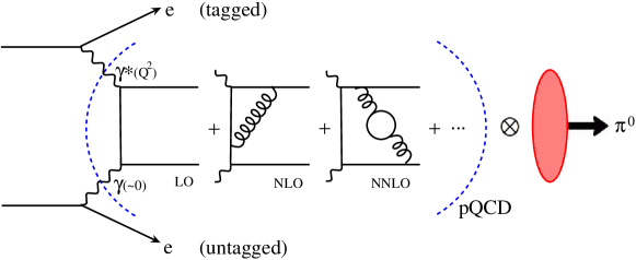
Figure 1: Schematic illustration of the single-tag $\pi^{0}$ production in a two-photon process with one photon having large virtuality $Q^{2}$, while the other, emitted from the untagged electron (positron), is almost real. The transition form factor for the process $\gamma^{*}\gamma\to q\bar{q}\to\pi^{0}$ is shown in factorized form in terms of a convolution (denoted by the symbol $\bigotimes$) which separates short- from long-distance dynamics. The former contributes to the hard-scattering amplitude, which is displayed in terms of some representative quark-gluon subprocesses in leading (LO), next-to-leading (NLO), and next-to-next-to-leading order (NNLO) of perturbative QCD (pQCD) within the parenthesis denoted by a dashed blue line. The solid (wavy) lines represent quarks (gluons). The nonperturbative long-distance part is encoded in the universal pion distribution amplitude denoted by the (red) shaded oval. Higher-twist contributions and the large-distance structure of the quasireal photon have been ignored here for simplicity; they are discussed in the text.

Using a single-tagged experimental set-up, one measures the differential cross section $d\sigma(Q^{2},q^{2}=0)/dQ^{2}$ for the above exclusive process by employing signal kinematics to select events in which the $\pi^{0}$ and one final-state electron (or positron) — the “tag” — are registered, while the other lepton remains undetected. Typically, one detects the decay products of the meson and either the electron (or the positron) which emerges after the scattering at some minimum angle relative to the $e^{+}e^{-}$ collision axis. In this case, one virtual photon has a large spacelike momentum (electron mass neglected)

$$Q^{2}\equiv-(p_{\text{beam}}-p_{\text{tag}})^{2}=2E_{\text{beam}}E_{\text{tag}}(1-\cos\theta_{\text{tag}})\,,$$ (2)

where $p_{\text{beam}}$ ($E_{\text{beam}}$) and $p_{\text{tag}}$ ($E_{\text{tag}}$) are the four-momenta (energies) of the incident beam-energy electron and the tag, respectively, with $\theta_{\text{tag}}$ being the scattering angle, while the other photon is almost real. Then, the differential cross section $d\sigma\left(e^{+}e^{-}\rightarrow e^{+}e^{-}R\right)/dQ^{2}$ can be linked to the TFF by employing the Budnev, Ginzburg, Meledin, and Serbo (BGMS) formalism Budnev et al. (1975). It states that the deviation of the production rate from the expression describing point-like pions as $Q^{2}$ grows, amounts to a measurement of the form factor. These considerations apply also to other processes $e^{+}e^{-}\to e^{+}e^{-}R$, where $R$ denotes one of the light pseudoscalar mesons $\pi^{0}$, $\eta$, $\eta^{\prime}$.

For these mesons, there is only one scalar form factor, which can be written in the form, see, e.g., Uehara et al. (2012a),

$$|F^{\gamma^{*}\gamma R}(Q^{2},q^{2}=0)|^{2}=\frac{d\sigma(Q^{2},q^{2}=0)/dQ^{2}}{2A(Q^{2})}\,,$$ (3)

where the quantity $A(Q^{2})$ is calculable within quantum electrodynamics (QED). At zero momentum transfer, $Q^{2}=0$, one has by normalization

$$|F^{\gamma^{*}\gamma R}(0,0)|^{2}=\frac{1}{(4\pi\alpha)^{2}}\frac{64\pi\Gamma(R\rightarrow\gamma\gamma)}{M_{R}^{3}}\,,$$ (4)

where $\alpha=1/137$ is the QED coupling constant, $\Gamma(R\rightarrow\gamma\gamma)$ is the two-photon partial width of the meson $R$ and $M_{R}$ is its mass. These two quantities are known from other experiments. The empirical form factor is extracted by comparing the measured values of the cross section with those from a Monte Carlo (MC) simulation,

$$F^{2}(Q^{2})=\frac{(d\sigma/dQ^{2})_{\text{data}}}{(d\sigma/dQ^{2})_{\text{MC}}}F_{\text{MC}}^{2}\,,$$ (5)

where $F_{\text{MC}}^{2}$ is a constant form factor. Typically, the two-photon Monte Carlo program in single-tag experiments is based on the BGMS formalism and describes the $Q^{2}$ (and $q^{2}$) development of the TFF by the following approximate form based on the factorization of the $Q^{2}$ and $q^{2}$ dependencies on account of vector meson dominance Sakurai (1960) (see, for instance, Gronberg et al. (1998a))

$$|F^{\gamma^{*}\gamma^{*}R}(Q^{2},q^{2})|^{2}\! \!\!\!=\frac{1}{(4\pi\alpha)^{2}}\frac{64\pi\Gamma(R\rightarrow\gamma\gamma)}{M_{R}^{3}}$$ (6)

$$\!\!\frac{1}{(1+Q^{2}/\Lambda_{R}^{2})^{2}}\frac{1}{(1+q^{2}/\Lambda_{R}^{2})^{2}}\,.$$

The pole-mass parameter $\Lambda_{R}\approx 770$ MeV is chosen to reproduce the momentum-transfer dependence of the form factors. Note that the calculated cross section $(d\sigma/dQ^{2})_{\text{MC}}$ acquires a model-dependent uncertainty induced by the unknown dependence on the momentum transfer to the untagged electron.

The behavior of the form factor is known theoretically in two limits. At $Q^{2}\to 0$ and in the chiral limit of quark masses, one obtains from the axial anomaly Adler (1969); Bell and Jackiw (1969)

$$\lim_{Q^{2}\to 0}F^{\gamma^{*}\gamma\pi^{0}}(Q^{2})=\frac{1}{2\sqrt{2}\pi^{2}f_{\pi}}\,,$$ (7)

where $f_{\pi}=132$ MeV is the leptonic decay constant of the pion. On the other hand, the asymptotic behavior of the form factor at $Q^{2}\to\infty$ is determined from perturbative QCD to be Lepage and Brodsky (1980); Brodsky and Lepage (1981)

$$\lim_{Q^{2}\to\infty}\mathcal{F}(Q^{2})=\sqrt{2}f_{\pi}\approx 0.187~{}\mbox{GeV}\,,$$ (8)

where we used the convenient notation

$$Q^{2}F^{\gamma^{*}\gamma\pi^{0}(Q^{2})}\equiv\mathcal{F}(Q^{2})\,.$$ (9)

The TFF in the $Q^{2}$ range between the aforementioned limits can be phenomenologically described by the interpolation formula of Brodsky and Lepage Brodsky and Lepage (1981),

$$F^{\gamma^{*}\gamma\pi}(Q^{2})=\frac{\sqrt{2}f_{\pi}}{4\pi^{2}f_{\pi}^{2}+Q^{2}}\ .$$ (10)

Analogous expressions hold for $\eta$ and $\eta^{\prime}$ with $f_{\pi}$ being replaced by the corresponding decay constants.

The asymptotic limit of the TFF at $Q^{2}\to\infty$ is the result of an abstraction process that cannot be realized in real-world experiments. To this end, one would need a long series of high-precision observations at higher and higher $Q^{2}$ values in order to minimize the influence of statistical flukes. Moreover, we don’t know at which momentum transfer the TFF should come close to the asymptotic limit. We also have no clues whether this limit is approached uniformly from below or from above; there is no sharp borderline between the underlying dynamical regimes. A selfconsistent calculation of the TFF within QCD encompasses various regimes of dynamics from low $Q^{2}\lesssim 1$ GeV², where perturbation theory is unreliable and nonperturbative effects are eventually more important but poorly known, up to high $Q^{2}$ values where one would expect that the perturbative contributions, depicted in Fig. 1 in terms of quark-gluon diagrams, prevail and provide an accurate dynamical picture within perturbative QCD. But again, there is no standard candle to fix a priori this crucial crossing point between nonperturbative and perturbative physics on route to collinear universality at $Q^{2}\to\infty$. For a broad survey of strong-interaction dynamics at different momentum scales, see Brambilla et al. (2014).

In fact, there are mainly three different sources of nonperturbative effects related to confinement that contribute to the TFF: (i) mass generation due to Dynamical Chiral Symmetry Breaking (DCSB), (ii) the bound-state dynamics of the pion, and (iii) the hadronic content of the quasireal photon that is emitted from the untagged electron (or positron) at large distances. We do not address DCSB in this work, but we refer to other approaches which account for this. A reliable theoretical scheme able to include the other two nonperturbative ingredients, together with higher-order perturbative QCD contributions and nonperturbative higher-twist corrections, is discussed in the next section.

Though such theoretical frameworks are extremely useful and embody the high principles of QCD, one needs in practice some guide for organizing and systematizing the data directly at the observational level, without appealing to underlying theoretical explanations at the level of quarks and gluons. This is even more important in the case of contradictory experimental data Aubert et al. (2009); Uehara et al. (2012a) that are eventually indicating discrepant observations applying to the same phenomenon; see Bakulev et al. (2012); Stefanis et al. (2013) for a detailed comparison of various theoretical approaches and a classification scheme of the predictions.

To extract dynamical information from the existing data on the experimental system, described by the quantity $\mathcal{F}(Q^{2})$, we employ for the first time in this field of physics a topology-based data analysis in terms of nonlinear time-series of measurements of this single scalar variable. The aim is to reconstruct the dynamical evolution of $\mathcal{F}(Q^{2})$ in terms of delay-coordinate maps from these time series that give rise to a trajectory representing the entirety of the states of this quantity. An introduction to the subject can be found in Williams (1997). To achieve this goal, we pursue the idea that the dynamical evolution of the system in its state space asymptotically contracts onto an unobservable attractor that can be reconstructed from scatter plots of delayed time series extracted from the data (measuring time in units of $Q^{2}$ [GeV²]). The key assumption is that some universal underlying determinism exists (related to the natural flow of the dynamical system), which may elude analysis using traditional methods in real space, but shows up in the pattern of the data in the form of an attractor in the lagged phase space of this quantity.

To reconstruct the phase-space portrait of the attractor, the time delay method pioneered by Packard et al. Packard et al. (1980) and independently by Takens Takens (1981) will be used. The delay method is based on the existence theorem for the embedding of manifolds in Euclidean spaces by Whitney Whitney (1936) and on Takens’ embedding theorem for delay-coordinate maps that provides a sufficient condition that the reconstructed attractor will have the same dynamical properties as the unobservable attractor of the full dynamical system of unknown dimension. These works were followed by the publication of an algorithm Grassberger and Procaccia (1983) to compute the correlation dimension of the reconstructed attractor, see Sauer et al. (1991) for a mathematical discussion of the embedding techniques and Hegger et al. (1999); Schreiber and Schmitz (2000); Pecora et al. (2007); Marwan et al. (2007); Bradley and Kantz (2015) for technical reviews. The concept of state-space reconstruction in terms of an attractor, has been widely used across a range of disciplines dealing with data that are generated sequentially in time, see Stam (2005).

The objective in this work is to identify a data-driven long-term pattern in the state-space of the physical TFF $\mathcal{F}(Q^{2})$ and use regular samplings of the existing experimental data to reconstruct an attractor in its state space. If the phase-state portrait of the reconstructed attractor exhibits a region of densely recurrent states in the vicinity of the asymptotic TFF value, given by Eq. (8), then this state aggregation quantified in terms of histograms, can be interpreted as a clear indication for a saturating behavior of the form factor in accordance with QCD. Such a phase-space configuration of the hypothesized attractor cannot be determined conclusively at present because, as we show in a later chapter, the number of the elements of the lagged time series, extracted from the available TFF data sets, is rather small at high $Q^{2}$. Nevertheless, replicating, grosso modo, the large-$Q^{2}$ QCD limit of the TFF by an accurate phase portrait of the quasi-asymptotic attractor directly from the data would not only provide a deeper theoretical insight how the onset of QCD scaling is approached, it would also deduce practical consequences for the data processing of future experiments. In fact, the main challenge in pursuing this methodology is the limited data coverage of the $10-25$ GeV² region, requiring a more dense data acquisition in steps of 1 GeV². Here the planned Belle-II experiment could contribute significantly in a momentum regime that offers a much better data-taking feasibility than the measurements at much higher $Q^{2}$ values. This option was barely explored in previous experiments.

The paper has two main parts. In the first part (Sec. II), we present theoretical predictions obtained within QCD using the method of light cone sum rules (LCSRs) Balitsky et al. (1989); Khodjamirian (1999) and fixed-order perturbation theory (FOPT). The spectral density at the twist two level includes all presently known radiative corrections up to the next-to-next-to-leading order Mikhailov et al. (2016). On the other hand, the twist-four term and the twist-six contribution Agaev et al. (2011) are also included. Note that the radiative corrections to the TFF can be taken into account in a resummed way by combining the LCSR method with the solution of the renormalization-group equation Ayala et al. (2018). Because in the present investigation we are mainly interested in the behavior of $\mathcal{F}(Q^{2})$ in the far-end $Q^{2}$ regime, where these effects play a minor role, we use for simplicity FOPT.

As nonperturbative input, we employ two types of endpoint-suppressed twist-two pion DAs: a family of bimodal DAs Bakulev et al. (2001) and a platykurtic DA determined more recently in Stefanis (2014) and further discussed in Stefanis et al. (2015); Stefanis and Pimikov (2016). Both types of DAs are obtained from QCD sum rules with nonlocal condensates (NLC). The latter have been introduced long ago in Mikhailov and Radyushkin (1986a); Mikhailov and Radyushkin (1989, 1990); Bakulev and Radyushkin (1991); Mikhailov and Radyushkin (1992). The mentioned DAs serve in the present analysis as a reference point to compare with TFF predictions obtained with external pion DAs within the same LCSR-based scheme. More explicitly, we derive predictions by employing the pion DAs determined with the help of Dyson-Schwinger equations (DSE) Chang et al. (2013); Raya et al. (2016), a light-front (LF) model Choi and Ji (2015), a nonlocal chiral quark model from the instanton vacuum Nam and Kim (2006), and from holographic AdS/QCD Brodsky et al. (2011a, b). To obtain the TFF at the measured $Q^{2}$ values, we use Efremov-Radyushkin-Brodsky-Lepage (ERBL) Efremov and Radyushkin (1980); Lepage and Brodsky (1980) evolution at the NLO, i.e., two-loop level, which includes heavy-quark thresholds (“global QCD scheme” Shirkov and Mikhailov (1994)). All calculated predictions are compared with the available data from the CELLO Behrend et al. (1991), CLEO Gronberg et al. (1998a), BABAR Aubert et al. (2009), and Belle Uehara et al. (2012a) experiments. The preliminary data of the BESIII Collaboration Redmer (2018) have also been included.

The second part of the paper is presented in Sec. III and is devoted to the analysis of the data from the last three mentioned experiments in the context of the state-space attractor reconstruction. The presentation includes the mathematical basis of the method and the techniques for its application in the present analysis. The key advantages of the reconstructed attractor in extracting information from the data on the dynamics of the $\pi-\gamma$ transition process are worked out. More importantly, it is shown that the phase-space attractor can provide a shortcut to uncover the asymptotic properties of the TFF from experiment at much lower $Q^{2}$ values than isolated measurements at much higher momenta. In Sec. IV, we examine and discuss more closely and critically the results obtained in the previous two main sections comparing them with estimates from lattice QCD. We summarize and conclude our analysis in Sec. V. The employed NLO evolution scheme with threshold inclusion is considered in Appendix A. The experimental data are displayed in Appendix B together with the values of the TFF and its chief uncertainties for the Bakulev-Mikhailov-Stefanis (BMS) set of DAs Bakulev et al. (2001). The analogous results for the platykurtic pion DA Stefanis (2014) are also included, employing in both cases the NLO evolution scheme worked out in the previous Appendix. These numerical values update all our previously published results.

II Theoretical analysis of $Q^{2}F^{\gamma^{*}\gamma\pi^{0}}(Q^{2})$ using LCSRs in QCD

In this section we consider the calculation of the pion-photon TFF using LCSRs Balitsky et al. (1989); Khodjamirian (1999) in QCD in conjunction with various pion DAs of twist two. We first expose the applied formalism Bakulev and Mikhailov (2002); Mikhailov and Stefanis (2009); Mikhailov et al. (2016) and then continue with the presentation and discussion of the obtained TFF predictions.

II.1 LCSR approach to the pion-photon transition form factor

In QCD, the amplitude $T_{\mu\nu}$ describing the process $\gamma^{*}(q_{1})\gamma^{*}(q_{2})\rightarrow\pi^{0}(P)$ (cf. (1)) is defined by the correlation function

$$\int\!d^{4}z\,e^{-iq_{1}\cdot z}\langle\pi^{0}(P)|T\{j_{\mu}(z)j_{\nu}(0)\}|0\rangle=i\epsilon_{\mu\nu\alpha\beta}q_{1}^{\alpha}q_{2}^{\beta}$$

$$~{}~{}~{}~{}~{}~{}~{}~{}~{}~{}~{}~{}~{}~{}\times~{}F^{\gamma^{*}\gamma^{*}\pi^{0}}(Q^{2},q^{2})\ ,$$ (11)

where $j_{\mu}=\frac{2}{3}\bar{u}\gamma_{\mu}u-\frac{1}{3}\bar{d}\gamma_{\mu}d$ is the quark electromagnetic current. Expanding the T-product of the composite (local) current operators in terms of $Q^{2}$ and $q^{2}$ (assuming that they are both sufficiently large, i.e., $Q^{2},~{}q^{2}\gg\Lambda_{R}^{2}$, cf. (6)), one gets by virtue of the factorization theorem, the LO term

$$F^{\gamma^{*}\gamma^{*}\pi}(Q^{2},q^{2})=N_{\text{T}}\int_{0}^{1}dx\frac{1}{Q^{2}\bar{x}+q^{2}x}~{}\varphi_{\pi}^{(2)}(x)$$ (12)

with $N_{\text{T}}=\sqrt{2}f_{\pi}/3$ and $\varphi_{\pi}^{(2)}$ denoting the pion DA of twist two. For vanishing $q^{2}$ it reduces to the expression

$$\frac{3}{\sqrt{2}f_{\pi}}Q^{2}F_{\gamma^{*}\gamma\pi^{0}}^{(\rm LO)}(Q^{2}) = \int_{0}^{1}\varphi_{\pi}^{(2)}(x)/x=\langle 1/x\rangle_{\pi}$$

$$= 3(1+a_{2}+a_{4}+a_{6}+\ldots)\,,$$

where we recast the inverse moment $\langle 1/x\rangle_{\pi}$ in terms of the projection coefficients $a_{n}$ on the set $\{\psi_{n}\}$ of the eigenfunctions of the one-loop ERBL evolution equation,

$$\varphi_{\pi}^{(2)}(x,\mu^{2})=\psi_{0}(x)+\sum_{n=2,4,\ldots}^{\infty}a_{n}(\mu^{2})\psi_{n}(x)\,.$$ (14)

Here $\psi_{0}(x)=6x(1-x)\equiv 6x\bar{x}$ is the asymptotic pion DA $\varphi_{\pi}^{\text{asy}}$ and the higher eigenfunctions are given in terms of the Gegenbauer polynomials $\psi_{n}(x)=6x\bar{x}C_{n}^{(3/2)}(x-\bar{x})$.

The pion DA parameterizes the matrix element

$$\langle 0|\bar{d}(z)\gamma_{\mu}\gamma_{5}[z,0]u(0)|\pi(P)\rangle|_{z^{2}=0} \!\!\!\!\!=if_{\pi}P_{\mu}\int_{0}^{1}dxe^{ix(z\cdot P)}$$ (15)

$$\times\varphi_{\pi}^{(2)}\left(x,\mu^{2}\right)\,,$$

where the path-ordered exponential (the lightlike gauge link) $[z,0]=\mathcal{P}\exp\left[ig\int_{0}^{z}t_{a}A_{a}^{\mu}(y)dy_{\mu}\right]$ ensures gauge invariance. It is set equal to unity by virtue of the light-cone gauge $z\cdot A=0$. Higher-twist DAs in the light cone operator product expansion of the correlation function in (11) give contributions to the TFF that are suppressed by inverse powers of $Q^{2}$. Physically, $\varphi_{\pi}^{(2)}(x,Q^{2})$ describes the partition of the pion’s longitudinal momentum between its two valence partons, i.e., the quark and the antiquark, with longitudinal-momentum fractions $x_{q}=x=(k^{0}+k^{3})/(P^{0}+P^{3})=k^{+}/P^{+}$ and $x_{\bar{q}}=1-x\equiv\bar{x}$, respectively. It is normalized to unity, $\int_{0}^{1}dx\varphi_{\pi}^{(2)}(x)=1$, so that $a_{0}=1$.

The expansion coefficients $a_{n}(\mu^{2})$ are hadronic parameters and have to be determined nonperturbatively at the initial scale of evolution $\mu^{2}$, but have a logarithmic $Q^{2}$ development via $\alpha_{s}(Q^{2})$ governed by the ERBL evolution equation, see, for instance, Stefanis (1999) for a technical review. The one-loop anomalous dimensions $\gamma_{n}^{(0)}$ are the eigenvalues of $\psi_{n}(x)$ and are known in closed form Lepage and Brodsky (1980). The ERBL evolution of the pion DA at the two-loop order is more complicated because the matrix of the anomalous dimensions is triangular in the $\{\psi_{n}(x)\}$ basis and contains off-diagonal mixing coefficients Dittes and Radyushkin (1981); Sarmadi (1984); Mikhailov and Radyushkin (1985); Müller (1994, 1995); Bakulev et al. (2003); Bakulev and Stefanis (2005); Agaev et al. (2011). To obtain the TFF predictions in the present work, we employ a two-loop evolution scheme, which updates the procedure given in Appendix D of Bakulev et al. (2003) by including the effects of crossing heavy-quark thresholds in the NLO anomalous dimensions $\gamma_{n}^{(1)}$ and also in the evolution of the strong coupling, see, e.g., Shirkov and Mikhailov (1994); Bakulev and Khandramai (2013); Ayala and Cvetič (2015) and App. A.

Elevating the convolution form (12) to higher orders, one has at the leading twist-two level Efremov and Radyushkin (1980); Lepage and Brodsky (1980)

$$F_{\text{QCD}}^{\gamma^{*}\gamma^{*}\pi^{0}}\!\!\left(Q^{2},q^{2},\mu_{\rm F}^{2}\right)= \!\!\!\!\!N_{\text{T}}\int_{0}^{1}dx\,T\left(Q^{2},q^{2};\mu_{\rm F}^{2};x\right)$$ (16)

$$\!\!\!\times\varphi_{\pi}^{(2)}\left(x,\mu_{\rm F}^{2}\right)+\mbox{h.t.}\,,$$

where $\mu_{\rm F}$ is the factorization scale between short-distance and large-distance dynamics and h.t. denotes higher-twist contributions. The hard-scattering amplitude $T$ has a power-series expansion in terms of the strong coupling $a_{s}\equiv\alpha_{s}(\mu_{\rm R}^{2})/4\pi$, where $\mu_{\text{R}}$ is the renormalization scale. In order to avoid scheme-dependent numerical coefficients, we set $\mu_{\text{F}}=\mu_{\text{R}}\equiv\mu$ (default choice). Hence we have

$$T\left(Q^{2},q^{2};\mu^{2};x\right)=T_{\text{LO}}+a_{s}~{}T_{\text{NLO}}+a_{s}^{2}~{}T_{\text{NNLO}}+\ldots\,,$$ (17)

where the short-distance coefficients on the right-hand side can be computed within FOPT in terms of Feynman diagrams as those depicted in Fig. 1. In our present calculation we include the following contributions, cast in convolution form via (16), and denoted by the symbol $\otimes\equiv\int_{0}^{1}dx$, where the convenient abbreviation $L\equiv\ln\left[\left(Q^{2}y+q^{2}\bar{y}\right)/\mu^{2}\right]$ is used Mikhailov and Stefanis (2009); Mikhailov et al. (2016),

$$\!T_{\rm LO} \!=\! T_{0},$$ (18a)

$$\!T_{\rm NLO} \!=\! C_{\rm F}~{}T_{0}\otimes\left[\mathcal{T}^{(1)}+L~{}V_{+}^{(0)}\right],$$ (18b)

$$\!T_{\rm NNLO} \!=\! C_{\rm F}T_{0}\otimes\!\left[\beta_{0}T_{\beta}+T_{\Delta V}+T_{L}+\mathcal{T}^{(2)}_{c}\right]\,.$$ (18c)

The dominant term is Melić et al. (2003); Mikhailov and Stefanis (2009)

$$T_{\beta}\! = \!\left[\mathcal{T}_{\beta}^{(2)}+L\left(V_{\beta+}^{(1)}-\mathcal{T}^{(1)}\right)-\frac{L^{2}}{2}V^{(0)}_{+}\right]\,,$$ (19)

where $\beta_{0}=\frac{11}{3}{\rm C_{A}}-\frac{4}{3}T_{\rm R}N_{f}$ is the first coefficient of the QCD $\beta$ function with $T_{\rm R}=1/2,{\rm C_{F}}=4/3,{\rm C_{A}}=3$ for $SU(3)_{c}$ and $N_{f}$ is the number of active flavors.

Two more contributions to the NNLO radiative corrections have been recently calculated in Mikhailov et al. (2016) to which we refer for their explicit expressions and further explanations. These are

$$T_{\Delta V} \!\!=\!\! L\Delta V^{(1)}_{+}\,,~{}~{}~{}\frac{V^{(1)}}{C_{\rm F}}=\beta_{0}V_{\beta}^{(1)}+\Delta V^{(1)}$$ (20a)

$$T_{L} \!\!=\!\! C_{\rm F}L\left[\frac{L}{2}V_{+}^{(0)}\otimes V_{+}^{(0)}+\mathcal{T}^{(1)}\otimes V_{+}^{(0)}\right]\,,$$ (20b)

while the term $\mathcal{T}_{c}^{(2)}$ in (18c) has not been computed yet and is considered in this work as the main source of theoretical uncertainties. Finally, suffices to say that $V_{+}^{(0)}$ and $V_{+}^{(1)}$ are the one- and two-loop ERBL evolution kernels, whereas $V_{\beta+}^{(1)}$ is the $\beta_{0}$ part of the two-loop ERBL kernel, with $\mathcal{T}^{(1)}$ and $\mathcal{T}_{\beta}^{(2)}$ denoting the one-loop and two-loop $\beta_{0}$ parts of the hard-scattering amplitude, respectively.

The TFF for one highly virtual photon with the hard virtuality $Q^{2}$ and one photon with a small virtuality $q^{2}\ll Q^{2}$ can be expressed within the LCSR approach in the form of a dispersion integral in the variable $q^{2}\rightarrow-s$, while $Q^{2}$ is kept fixed, to obtain

$$F_{\text{LCSR}}^{\gamma^{*}\gamma^{*}\pi^{0}}\left(Q^{2},q^{2}\right)=N_{\text{T}}\int_{0}^{\infty}ds\frac{\rho(Q^{2},s)}{q^{2}+s}\,,$$ (21)

where $\rho(Q^{2},s)$ is the spectral density

$$\rho(Q^{2},s)=\rho^{\text{h}}(Q^{2},s)\theta(s_{0}-s)+\rho^{\text{pert}}(Q^{2},s)\theta(s-s_{0})\,.$$ (22)

The first term $\rho^{\text{h}}(Q^{2},s)$ models the hadronic (h) content of the spectral density,

$$\rho^{\text{h}}(Q^{2},s)=\sqrt{2}f_{\rho}F^{\gamma^{*}\rho\pi}(Q^{2})\delta(s-m_{\rho}^{2})\,,$$ (23)

while $\rho^{\text{pert}}(Q^{2},s)$ denotes the QCD part in terms of quarks and gluons, calculable within perturbative QCD,

$$\rho^{\text{pert}}(Q^{2},s) = \frac{1}{\pi}\text{Im}F_{\text{QCD}}^{\gamma^{*}\gamma^{*}\pi^{0}}(Q^{2},-s,-i\epsilon)$$ (24)

$$= \rho_{\text{tw-2}}+\rho_{\text{tw-4}}+\rho_{\text{tw-6}}+\ldots\,.$$

Each of these terms can be computed from the convolution of the associated hard part with the corresponding DA of the same twist (tw for short) Khodjamirian (1999). Below some effective hadronic threshold in the vector-meson channel, the photon emitted at large distances is replaced in $F^{\gamma^{*}V\pi^{0}}$ by a vector meson $V=\rho$, $\omega$, etc., using for the corresponding spectral density a phenomenological ansatz, for instance, a $\delta$-function model.

Thus, after performing the Borel transformation $1/(s+q^{2})\rightarrow\exp\left(-s/M^{2}\right)$, with $M^{2}$ being the Borel parameter, one obtains the following LCSR (see Agaev et al. (2011); Mikhailov and Stefanis (2009); Mikhailov et al. (2016) for more detailed expositions)

$$Q^{2}F_{\text{LCSR}}^{\gamma*\gamma*\pi^{0}}\left(Q^{2},q^{2}\right)=N_{\text{T}}f_{\pi}\left[\frac{Q^{2}}{m_{\rho}^{2}+q^{2}}\int_{x_{0}}^{1}\exp\left(\frac{m_{\rho}^{2}-Q^{2}\bar{x}/x}{M^{2}}\right)\bar{\rho}(Q^{2},x)\frac{dx}{x}+\!\int_{0}^{x_{0}}\bar{\rho}(Q^{2},x)\frac{Q^{2}dx}{\bar{x}Q^{2}+xq^{2}}\right]\,,$$ (25)

where the spectral density is given by

$$\bar{\rho}(Q^{2},s)=(Q^{2}+s)\rho^{\text{pert}}(Q^{2},s)\,.$$ (26)

For simplicity, we have shown the LCSR expression above using the simple $\delta$-function model to include the $\rho$-meson resonance into the spectral density. However, the actual calculation of the TFF predictions to be presented below, employs a more realistic Breit-Wigner form, as suggested in Khodjamirian (1999) and used in Mikhailov and Stefanis (2009),

$$\delta(s-m_{\text{V}}^{2})\longrightarrow\Delta_{\text{V}}(s)\equiv\frac{1}{\pi}\frac{m_{\text{V}}\Gamma_{\text{V}}}{(m_{\text{V}}^{2}-s)^{2}+m_{\text{V}}^{2}\Gamma_{\text{V}}^{2}}\,,$$ (27)

where the masses and widths of the $\rho$ and $\omega$ vector mesons are given by $m_{\rho}=0.770$ GeV, $m_{\omega}=0.7826$ GeV, $\Gamma_{\rho}=0.1502$ GeV, and $\Gamma_{\omega}=0.00844$ GeV, respectively. The other parameters entering (25) are $s=\bar{x}Q^{2}/x$ with $\bar{x}\equiv 1-x$, $x_{0}=Q^{2}/\left(Q^{2}+s_{0}\right)$, and the effective threshold in the vector channel $s_{0}\simeq 1.5$ GeV². The stability of the LCSR is ensured for values of the Borel parameter $M^{2}$ in the interval $M^{2}\in[0.7-1.0]$ GeV² Bakulev et al. (2011, 2012); Stefanis et al. (2013); Mikhailov et al. (2016). By allowing a stronger variation towards larger values $M^{2}\in[0.7-1.5]$ GeV² Agaev et al. (2011, 2012), the TFF prediction receives an uncertainty of the order $[-1.6-7.2]\%$ Mikhailov et al. (2016). Note at this point that the LCSR in (25) includes in an effective way the nonperturbative long-distance properties of the real photon in terms of the duality interval $s_{0}$ and the masses of the vector mesons that are absent in the pQCD formulation of the TFF, but play an important role in the kinematic region $Q^{2}\lesssim s_{0}$ and $x_{0}\lesssim 0.5$ (cf. the first term in Eq. (25)).

One appreciates that the real-photon limit $q^{2}\to 0$ can be taken in (25) by simple substitution because there are no massless resonances in the vector-meson channel. Thus, this equation correctly reproduces the behavior of the TFF for a highly virtual and a quasireal photon from the asymptotic limit $Q^{2}\rightarrow\infty$ down to the hadronic normalization scale of $Q^{2}\sim 1$ GeV².

Using the conformal expansion for $\rho_{\text{tw-2}}$, the spectral density can be expressed in the form

$$\bar{\rho}\left(Q^{2},x\right)= \!\!\!\sum_{n=0,2,4,\ldots}a_{n}\left(Q^{2}\right)\bar{\rho}_{n}\left(Q^{2},x\right)+\bar{\rho}_{\text{tw-4}}\left(Q^{2},x\right)$$ (28)

$$+\bar{\rho}_{\text{tw-6}}\left(Q^{2},x\right)+\ldots\,,$$

where

$$\bar{\rho}_{n}\left(Q^{2},x\right)\!\!\! \!\!=\!\! \!\!\!\bar{\rho}_{n}^{(0)}(x)\!\!+\!a_{s}\bar{\rho}_{n}^{(1)}(Q^{2},x)\!\!+\!a_{s}^{2}\bar{\rho}_{n}^{(2)}(Q^{2},x)+\ldots,$$

$$\bar{\rho}_{n}^{(0)}(x) = \psi_{n}(x);~{}\,a_{s}=a_{s}(Q^{2})\,,$$ (29)

with the elements $\bar{\rho}_{n}^{(i)}$ being given in Appendix B of Ref. Mikhailov et al. (2016).

The dispersive analysis here includes the twist-four and twist-six spectral densities in explicit form, as done in Mikhailov et al. (2016). The $\bar{\rho}_{\text{tw-4}}$ spectral density is given by

$$\bar{\rho}_{\text{tw-4}}(Q^{2},x)=\frac{\delta^{2}_{\text{tw-4}}(Q^{2})}{Q^{2}}x\frac{d}{dx}\varphi^{(4)}(x)\Bigg{|}_{x=Q^{2}/(Q^{2}+s)}\,,$$ (30)

where the twist-four coupling parameter takes values in the range $\delta^{2}_{\text{tw-4}}(\mu^{2}=1~{}\rm{GeV}^{2})\approx\lambda_{q}^{2}/2=0.19\pm 0.04$ GeV² and is closely related to the average virtuality $\lambda_{q}^{2}$ of vacuum quarks Mikhailov and Radyushkin (1986a); Mikhailov and Radyushkin (1989, 1990); Bakulev and Radyushkin (1991); Mikhailov and Radyushkin (1992), defined by $\lambda_{q}^{2}\equiv\langle\bar{q}(ig\sigma_{\mu\nu}G^{\mu\nu})q\rangle/(2\langle\bar{q}q\rangle)=0.4\pm 0.05~{}\text{GeV}^{2}$. Details on its estimation and evolution can be found in Bakulev et al. (2003), whereas the sensitivity of the TFF to its variation was examined in Bakulev et al. (2004a). In the present analysis the evolution of $\delta^{2}_{\text{tw-4}}$ is also included. Expression (30) is evaluated with the asymptotic form of the twist-four pion DA Khodjamirian (1999)

$$\varphi_{\pi}^{(4)}(x,\mu^{2})=\frac{80}{3}\delta^{2}_{\text{tw-4}}(\mu^{2})x^{2}(1-x)^{2}\,,$$ (31)

while more complicated forms were considered in Agaev (2005); Bakulev et al. (2006). The twist-six part of the spectral density, i.e., $\bar{\rho}_{\text{tw-6}}(Q^{2},x)=(Q^{2}+s)\rho_{\text{tw-6}}(Q^{2},s)$, was first derived in Agaev et al. (2011). An independent term-by-term calculation in Mikhailov et al. (2016) provided the same result, which we quote here in the form

$$\bar{\rho}_{\text{tw-6}}(Q^{2}\!,x)=8\pi\frac{C_{\text{F}}}{N_{c}}\frac{\alpha_{s}\langle\bar{q}q\rangle^{2}}{f_{\pi}^{2}}\frac{x}{Q^{4}}\left[\!-\!\left[\frac{1}{1-x}\right]_{+}\!+\!\left(2\delta(\bar{x})-4x\right)\!+\!\left(3x+2x\log{x}\!+\!2x\log{}\bar{x}\right)\right]\,,$$ (32)

where the plus prescription $[f(x,y)]_{+}=f(x,y)-\delta(x-y)\int_{0}^{1}f(z,x)dz$ is involved, while $\alpha_{s}=0.5$ and $\langle\bar{q}q\rangle^{2}=\left(0.242\pm 0.01\right)^{6}$ GeV⁶ Gelhausen et al. (2013).

To obtain detailed numerical results for the TFF $\mathcal{F}(Q^{2})$ using (25), we employ several DAs from different approaches with various shapes encoded in their conformal coefficients $a_{n}$. The latter are determined at their native normalization scale (as quoted in the referenced approaches) by means of the moments of the pion DA

$$\langle\xi^{N}\rangle_{\pi}\equiv\int_{0}^{1}\varphi_{\pi}^{(2)}(x,\mu^{2})(x-\bar{x})^{N}dx\,,$$ (33)

where $\xi=x-\bar{x}$ and $N=2,4,\ldots$. The expansion coefficients $a_{n}$ can be expressed in terms of the moments $\langle\xi^{N}\rangle_{\pi}$ as follows

$$a_{2n}=\frac{2}{3}\frac{4n+3}{(2n+1)(2n+2)2^{2n}}\sum_{m=0}^{n}(-1)^{(n-m)}\frac{\Gamma(2n+2m+2)}{\Gamma(n+m+1)\Gamma(n-m+1)\Gamma(2m+1)}\langle\xi^{2m}\rangle_{\pi}~{}~{}~{}~{}~{}(n=0,1,2,3\ldots)\,.$$ (34)

Table 1: Conformal coefficients $a_{2}$, $a_{4}$, $a_{6}$ for various pion DAs discussed in the text at two typical hadronic momentum scales $\mu_{1}=1$ GeV and $\mu_{2}=2$ GeV. If $\mu_{2}$ is not the initial scale, NLO ERBL evolution in the global scheme is employed as explained in the text and in Appendix A. The errors of the BMS DA given below are related to the determination of $a_{2}$ and $a_{4}$ from QCD sum rules with nonlocal condensates. They cause the variation of the TFF predictions shown in the form of a green shaded band in Figs. 2 and 3. Note that the coefficient $a_{2}$ of the CZ DA was originally given at the scale $\mu=0.5$ GeV: $a_{2}^{\text{CZ}}=2/3$ Chernyak and Zhitnitsky (1984). The detailed procedure how to evaluate it at higher scales is described in Appendix B of Ref. Bakulev et al. (2003). Higher conformal coefficients up to and including $a_{12}$ for the DSE-DB and DSE-RL DAs at the scale $\mu_{2}$ can be found in Raya et al. (2016). For the holographic AdS/QCD DA $\varphi_{\pi}^{\text{hol}}(x)=(8/\pi)\sqrt{x\bar{x}}$ the coefficients up to and including $a_{20}$ at the scale $\mu_{1}$ are tabulated in Brodsky et al. (2011a). They are calculable by means of the expression $\left\langle\xi^{2n}\right\rangle_{\pi}^{\text{AdS/QCD}}=\frac{1}{4}\frac{B\left(3/2,(2n+1)/2\right)}{B(3/2,3/2)}$ [$B(x,y)$ being the Euler Beta function] in combination with Eq. (34). The symbol (?) in the lattice result of Braun et al. (2015) indicates that it was not extrapolated to the continuum limit. The lattice results of Bali et al. (2019) at NNLO and NLO are quoted separately. They were obtained from a combined extrapolation to the chiral and continuum limit.

Pion DA	$a_{2}(\mu_{1})$	$a_{4}(\mu_{1})$	$a_{6}(\mu_{1})$	$a_{2}(\mu_{2})$	$a_{4}(\mu_{2})$	$a_{6}(\mu_{2})$	$\langle 1/x\rangle(\mu_{2})$
BMS Bakulev et al. (2001); Mikhailov et al. (2016)	$0.203_{-0.057}^{+0.069}$	$-0.143_{-0.087}^{+0.094}$	0	$0.149_{-0.043}^{+0.052}$	$-0.096_{-0.058}^{+0.063}$	0	$3.16^{+0.09}_{-0.09}$
BMS range	$[0.146,0.272]$	$[-0.23,-0.049]$	0	$[0.11,0.20]$	$[-0.15,-0.03]$	0	–
platykurtic Stefanis (2014)	$0.0812_{-0.025}^{+0.0345}$	$-0.0191_{-0.0287}^{0.0337}$	0	$0.057^{+0.024}_{-0.019}$	$-0.013^{+0.022}_{-0.019}$	0	$3.13^{+0.14}_{-0.10}$
platykurtic range	$[0.0562,0.1156]$	$[-0.0478,0.0147]$	0	$[0.04,0.08]$	$[-0.03,0.01]$	0	–
DSE-DB Chang et al. (2013)	–	–	–	0.149	0.076	0.031	4.6
DSE-RL Chang et al. (2013)	–	–	–	0.233	0.112	0.066	5.5
AdS/QCD Brodsky et al. (2011a)	$7/48$	$11/192$	$5^{3}/2^{12}$	0.107	0.038	0.0183	4.0
Light-Front QM Choi and Ji (2015)	0.0514	-0.0340	-0.0261	0.035	$-0.0227$	-0.0153	2.99
NL$\chi$ QM Nam and Kim (2006)	0.0534	-0.0609	-0.0260	0.037	$-0.041$	-0.015	3.18
CZ (this work)	0.56	0	0	0.412	0	0	4.25
Lattice Braun et al. (2015)	–	–	–	0.1364(154)(145)(?)	–	–	–
Lattice (NNLO) Bali et al. (2019)	–	–	–	$0.099^{+17}_{-17}(11)(11)(5)$	–	–	–
Lattice (NLO) Bali et al. (2019)	–	–	–	$0.076^{+19}_{-18}(18)(12)(4)$	–	–	–

II.2 Parton-level predictions for the TFF

Let us now outline the calculational procedure to obtain predictions for the scaled TFF $\mathcal{F}(Q^{2})$ within our LCSR scheme using as nonperturbative input the various pion DAs given in Table 1 in terms of their conformal coefficients $a_{2},a_{4},a_{6}$ at the scales $\mu_{1}=1$ GeV and $\mu_{2}=2$ GeV. If $\mu_{2}$ is not the original normalization scale of a DA, NLO evolution in the global scheme (see App. A) is applied. The number of the conformal coefficients included in the TFF calculation depends on the particular shape of the DA. For the two types of DAs derived from QCD sum rules with nonlocal condensates, notably, the bimodal BMS DA Bakulev et al. (2001) and the platykurtic DA Stefanis (2014), a two-parametric form involving the lowest two nontrivial coefficients $a_{2}$ and $a_{4}$ is sufficient. Note that these DAs correspond to slightly different but admissible values of the average vacuum-quark virtuality, $\lambda_{q}^{2}(\mu^{2}\approx 1~{}\mbox{GeV}^{2})=0.4$ GeV² and $\lambda_{q}^{2}(\mu^{2}\approx 1~{}\mbox{GeV}^{2})=0.45$ GeV², respectively; they both have suppressed endpoint regions $x=0,1$. The motivation underlying the construction of the platykurtic DA Stefanis (2014) originates from the desire to find a DA that generically combines the implications of the vacuum nonlocality with the dynamical mass dressing of the confined quark due to the DCSB. The DA with a short-tailed platykurtic profile represents the optimal realization of this task within the space of the conformal expansion using QCD sum rules with nonlocal condensates, see Fig. 2 in Stefanis and Pimikov (2016).

Unimodal DAs with more or less suppressed tails have been obtained in other approaches as well. Recent examples are the light-front (LF) quark model (QM) of Choi and Ji (2015) and the spin-improved holographic model of Ahmady et al. (2017a, b). It is worth reminding in this context that arguments to support the suppression of the endpoint regions of the pion DA were already given in Stefanis et al. (1999, 2000); Nam and Kim (2006); Choi and Ji (2007) in the context of quantum fluctuations of the QCD (instanton) vacuum and the appearance of fermionic zero modes.

By contrast, the calculation of the LO and NLO terms of the TFF with broad unimodal DAs with heavy tails, requires the inclusion of all coefficients up to $a_{12}$, see the right panel of Fig. 2 in Stefanis et al. (2015), though in our approach the contribution of $a_{12}$ is only about $0.2\%$ Stefanis et al. (2015). Examples of such pion DAs are those derived from the Dyson-Schwinger equations (DSE) approach of Ref. Chang et al. (2013) (DSE-DB and DSE-RL), where DB stands for the most advanced Bethe-Salpeter kernel and RL denotes the rainbow ladder approximation. The broad shapes of these DAs are attributed to DCSB Chang et al. (2013); Raya et al. (2016). A similarly concave pion DA with a somewhat narrower profile was determined in the framework of holographic AdS/QCD Brodsky et al. (2011a, b). These three DAs together with the platykurtic one agree well with the sum-rule estimate $\varphi_{\pi}^{\text{SR}}(x=1/2)=1.2\pm 0.3$ computed in Braun and Filyanov (1989) (see Stefanis et al. (2015) for the numerical values). A comparative illustration of the shapes of some of the mentioned pion DAs can be found in Stefanis and Pimikov (2016). The corresponding graphic representations for the TFF are shown in Fig. 2, where the simplified notation $Q^{2}F_{\gamma\pi}(Q^{2})$ is used. These TFF predictions have been obtained by applying the NLO evolution scheme with varying heavy flavors discussed in App. A. This scheme works for an arbitrary number of Gegenbauer coefficients, so that such broad DAs can be evolved appropriately. This figure is supplemented by Table 2 in App. B, where we supply the data from the CELLO Behrend et al. (1991), CLEO Gronberg et al. (1998a), BABAR Aubert et al. (2009), and Belle Uehara et al. (2012a) experiments. The preliminary BESIII data can be found in graphical form in Redmer (2018), see also Danilkin et al. (2019).

We now consider our results more systematically.

(i) The range of the $\mathcal{F}(Q^{2})$ values, obtained with the set of the BMS DAs Bakulev et al. (2001), is illustrated in Fig. 2 by means of a green shaded band, whereas the prediction derived with the platykurtic DA Stefanis (2014) is denoted by a single solid black line. This is because, as quantified in Stefanis and Pimikov (2016), the margin of variation of $a_{2}$ and $a_{4}$ for the platykurtic pion DA is much smaller than that for the BMS DA, entailing uncertainties for the TFF that are covered by those obtained with the BMS set of DAs. Note, however, that the corresponding domains in the $(a_{2},a_{4})$ space do not overlap, see Table 1 and Fig. 2 in Stefanis and Pimikov (2016). The calculation of the twist-two part of the TFF with the BMS DAs and the platykurtic one includes the LO, NLO, and NNLO-$T_{\beta_{0}}$ contributions to the short-distance coefficients, cf. (18), (19), at the $\{\psi_{0},\psi_{2},\psi_{4}\}$ level of the conformal expansion. The $\psi_{0}$ eigenfunction yields the largest (negative) NNLO-$T_{\beta_{0}}$ contribution. Therefore, also the term $T_{\Delta V}\ll T_{\beta_{0}}$, cf. (20a), is taken into account only via the zero harmonic $\psi_{0}$. Finally, the term NNLO-$T_{L}$ vanishes for $\psi_{0}$, cf. (20b) Mikhailov et al. (2016). The remaining NNLO term $T_{c}$ is unknown and this unknownness induces the dominant theoretical uncertainty in the TFF prediction (blue strip enveloping the green one). To estimate it, we assume that this term may be comparable in magnitude to the leading NNLO term $T_{\beta_{0}}$ (which actually means that its potential influence is likely to be overestimated). This main theoretical uncertainty, computed with the BMS DAs via the coefficients $a_{2}$ and $a_{4}$ at each measured value of the TFF, is included in Table 2. The analogous errors for the platykurtic DA are within these intervals and have been omitted. Estimates of further theoretical errors can be found in Mikhailov et al. (2016), whereas the influence on the TFF predictions of the virtuality of the untagged photon has been determined within our LCSR approach in Stefanis et al. (2013). This effect yields suppression at all momentum scales and diminishes at high $Q^{2}$ so that it has little influence on our considerations regarding the long-term $Q^{2}\to\infty$ behavior of the TFF. The total TFF comprises in the spectral density (28) the contributions (30) (twist four) and (32) (twist six). The uncertainties induced by these terms were estimated in Mikhailov et al. (2016), see also Mikhailov et al. (2017). They are not included in the presented predictions in Fig. 2 because they do not affect them qualitatively at large $Q^{2}$. Also the explicit inclusion of the small coefficient $a_{6}$ in the conformal expansion of the BMS DA does not modify the TFF prediction markedly but contributes to the theoretical noise Stefanis et al. (2013). We do not consider this effect here. This notwithstanding, the inclusion of a third coefficient in the TFF calculation increases the overlap between the BMS-based prediction (green shaded band in Fig. 2) and the Belle data at high $Q^{2}$ Stefanis et al. (2013).

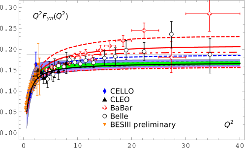
Figure 2: Measurements of the scaled pion-photon transition form factor $Q^{2}F_{\gamma\pi}(Q^{2})$ from different experiments, with labels as indicated, in comparison with theoretical predictions obtained with various pion DAs in LCSRs. The innermost green shaded strip shows the range of predictions pertaining to the set of the bimodal BMS DAs from Bakulev et al. (2001), with the thick black line inside it denoting the result for the platykurtic DA Stefanis (2014). The wider band (in blue color) around the strip encapsulates the principal theoretical uncertainty owing to the unknown NNLO term $T_{c}$ (see the text for explanations). The upper two red lines illustrate the predictions from the DSE approach: DSE-DB Chang et al. (2013) (solid line) and DSE-RL Chang et al. (2013) (dashed line). The dashed-dotted-dotted red line denotes the prediction obtained for the DSE-DB DA using a lower conformal resolution (only $\{a_{2},a_{4}\}$). The dashed blue line below it represents the result derived from AdS/QCD Brodsky and de Téramond (2008), whereas the solid pink line and the red dashed-dotted line below the lower boundary of the total BMS band show the predictions calculated with a light-front-based field theoretical quark model Choi and Ji (2015) and an instanton-based chiral quark model Nam and Kim (2006), respectively. The horizontal solid line marks the asymptotic limit $\mathcal{F}_{\infty}\approx 0.187$ GeV following from perturbative QCD, cf. Eq. (8).

(ii) The dashed red line farthest above the asymptotic limit (horizontal black line) in Fig. 2 shows the $\mathcal{F}(Q^{2})$ prediction for the DSE-RL DA Chang et al. (2013), whereas the solid red line below it exposes the result for the DSE-DB DA Chang et al. (2013). The corresponding twist-two TFF predictions were obtained by incorporating the LO and NLO contributions using the set $\{a_{2},a_{4},\ldots,a_{12}\}$. The values of these conformal coefficients at the initial scale $\mu_{2}$ are taken from Raya et al. (2016). The NNLO term $T_{\beta_{0}}$ is sufficiently included by means of the smaller set of coefficients $\{a_{2},a_{4},a_{6}\}$, given in Table 1. This restricted treatment already embodies over 96 percent of the total TFF, see Fig. 2 (right panel) in Stefanis et al. (2015). The other two NNLO terms, $T_{\Delta V}$ and $T_{L}$, are treated as in item (i). The contributions of the partial NNLO terms for the various Gegenbauer eigenfunctions $\psi_{n}(x)$ have been examined in Mikhailov et al. (2016)—see Fig. 2 and Appendix B there. The long-dashed-dotted-dotted red line shows the prediction for the TFF involving the DSE-DB DA with a lower conformal resolution that relies only upon the coefficients $a_{2}$ and $a_{4}$. As one sees, this prediction agrees better with the asymptotic limit, despite the fact that the reduced set of conformal coefficients represents a rather crude approximation of the broad shape of the DSE-DB DA Raya et al. (2016) given by $\varphi_{\pi}^{\text{DSE-DB}}(x)=N_{\alpha}^{\text{DB}}[x\bar{x}]^{\alpha_{-}^{\text{DB}}}[1+a_{2}^{\text{DB}}C_{2}^{\alpha_{-}^{\text{DB}}+1/2}(x-\bar{x})]$, where $N_{\alpha}^{\text{DB}}=1.81$, $\alpha_{-}^{\text{DB}}=0.31$, $a_{2}^{\text{DB}}=-0.12$. Thus, the inclusion of a large number of conformal coefficients in unimodal DAs with enhanced endpoint regions may have a detrimental effect on the quality of the TFF prediction inside our LCSR-based scheme.

(iii) The computation of the TFF for the holographic DA Brodsky et al. (2011a) proceeds along the lines described in the previous item. The twist-two part includes at the LO+NLO level all coefficients $\{a_{2},\ldots,a_{12}\}$, whereas at the NNLO, the $T_{\beta_{0}}$ contribution comprises $(a_{2},a_{4},a_{6})$, the term $T_{\Delta V}$ includes only $a_{0}$, whereas $T_{L}=0$ and $T_{c}$ is unknown, contributing an unestimated theoretical error. The result for $\mathcal{F}(Q^{2})$ is displayed in Fig. 2 in terms of a dashed blue line running close to the asymptotic limit above 10 GeV² and approaching it fast from below. The first three coefficients $\{a_{2},a_{4},a_{6}\}$ of this DA are given in Table 1 at both scales $\mu_{1}$ and $\mu_{2}$ using NLO ERBL evolution in the global scheme to connect them. It is worth noting that there is a misprint in Table II of Brodsky et al. (2011a). The coefficients starting with order 10 up to 20 are actually one order lower, i.e., 8 to 18. For the convenience of the reader, we supply here the missing coefficient at $\mu_{1}$: $a_{20}(\mu_{1}=1~{}\text{GeV})=0.0037$.

(iv) Figure 2 includes the TFF derived within our approach with the light-front quark model (LFQM) from Choi and Ji (2015) in terms of a solid line in pink color below the blue strip. The calculation takes into account at the twist two level the LO and NLO contributions, as well as the radiative correction induced by the term NNLO-$T_{\beta_{0}}$ using as a nonperturbative input the conformal coefficients $\{a_{2},a_{4},a_{6}\}$, computed by the authors at the initial scale $\mu_{1}$ (see Table II in Choi and Ji (2015)). The numerical values of these coefficients at $\mu_{2}$, shown in Table 1 and used in our graphics, were obtained with NLO ERBL evolution in the global scheme. The other NNLO term, notably, $T_{\Delta V}$, is included for the zero harmonic, whereas, as before, $T_{L}=0$, and the error induced by the unknown contribution $T_{c}$ is ignored.

(v) Table 1 also contains the conformal coefficients $\{a_{2},a_{4},a_{6}\}$ of the nonlocal chiral quark model (NL$\chi$QM) from Nam and Kim (2006) (model 3 in their Table II) at the two scales $\mu_{1}$ and $\mu_{2}$ (the latter after NLO evolution in the global scheme). The intrinsic scale of this model is actually lower than $\mu_{1}$, but we follow the line of reasoning given by the authors to show the conformal coefficients at the normalization scale $\mu_{1}$ (dubbed $\Lambda_{1}$ in their terminology) with their original values Nam and Kim (2006). One observes from Table 1 that these coefficients are quite close to those of the light-front quark model Choi and Ji (2015) treated in item (iv). As a result, the obtained TFF prediction (dashed-dotted red line below all other curves) in Fig. 2 practically coincides with the LFQM one (solid pink line just above it).

(vi) We shortly comment here on the recent lattice results for the second Gegenbauer moment from Bali et al. (2019). The quoted values were obtained from a combined chiral and continuum limit extrapolation at the NNLO (two-loops) and NLO (one-loop). The corresponding central values deviate considerably from each other. This treatment differs from that applied in Braun et al. (2015), where no extrapolation to the continuum limit was carried out. This is indicated by the label (?) in Table 1. From this table one observes that the following DAs have $a_{2}(\mu_{2})$ coefficients coming close to the NNLO value (deviation in parenthesis): AdS/QCD (0.008), platykurtic (-0.042), NL$\chi$QM (-0.062), and LFQM (-0.064). As we will see later in terms of Figs. 2, 3 more explicitly, the first of these DAs yields a TFF prediction that approaches fast $\mathcal{F}_{\infty}$ and, depending on the number of the conformal coefficients included in the calculation, eventually crosses it around 60 GeV². The other three DA models lead to predictions that remain below this limit, with the platykurtic DA giving a TFF closest to $\mathcal{F}_{\infty}$ and approaching it uniformly from below. We mention without further discussion that the new lattice NNLO result agrees with the value found in Agaev et al. (2012) by fitting model II Agaev et al. (2011) to the Belle data instead of BABAR. This model gives $a_{2}=a_{4}=a_{6}=0.10$, while $a_{8}=0.034$. It is worth noting that the previous lattice estimate Braun et al. (2015) was quite larger (0.136) and close to the value $a_{2}(\mu_{2})=0.140$ for the mentioned model II, but also not far away from the DSE-DB and the BMS DA, which both give 0.149 (Table 1). Within the reported uncertainties, all these DAs are reasonable candidates and cannot be differentiated by this single constraint.

II.3 Asymptotic behavior of the calculated TFF

Going further, we now give a broader discussion of the various TFF predictions, founded upon the main observations from Fig. 2, focusing our attention on their asymptotic behavior.

a) Pion DAs, like the BMS set Bakulev et al. (2001) (narrower green strip) and the platykurtic one Stefanis (2014) (solid black line inside it), which implicitly incorporate a nonvanishing average virtuality of the vacuum quarks, have suppressed tails at $x=0,1$ — irrespective of their topology at the central point $x=1/2$ (bimodal the first, unimodal the second). This suppression entails a balanced magnitude of the scaled TFF so that it approaches with increasing $Q^{2}$ the QCD asymptotic limit monotonically from below, being at the same time in good overall agreement within the margin of experimental and theoretical error with those data that support QCD scaling at large $Q^{2}$. More specifically, the predictions for $\mathcal{F}(Q^{2})$ herewith follow the steep rise indicated by all existing data below 4 GeV² and start to scale with $Q^{2}$ above about 8 GeV². The magnitude of the scaled TFF tends toward $\mathcal{F}_{\infty}$ very slowly from below. Both types of DAs comply with the BABAR data below 10 GeV² but deviate from them significantly above this mark (except at $Q^{2}=27.31$ GeV² where they agree). They are also overall consistent with the Belle data — except at $Q^{2}=34.36$ GeV² where they fall short. In aggregate, the BMS band of the TFF predictions can accommodate within the margin of experimental error all data below 15 GeV². Note that the TFF prediction obtained with the Chernyak-Zhitnitsky pion DA (not shown in Fig. 2) exceeds all data considerably already in the region of a few GeV² and scales then towards higher $Q^{2}$ values, crossing the BABAR branch at 22.28 GeV² and the Belle measurement at 27.33 GeV² (see Bakulev et al. (2012) for a graphic illustration and Wang and Shen (2017) for a different conclusion using another approach).

b) As we already mentioned, the LFQM-based DA Choi and Ji (2015); Choi et al. (2017) yields a TFF prediction (solid pink line) that exhibits a $Q^{2}$ behavior similar to that obtained with the BMS/platykurtic DA, albeit with a somewhat smaller magnitude. Also the NL$\chi$QM DA Nam and Kim (2006) yields a TFF (dashed-dotted red line) which replicates this result. The root for this proximity of predictions can be traced to the similar profiles of the underlying pion DAs. However, there is a crucial difference. While the platykurtic DA has $a_{6}=0$, the other two models involve a negative $a_{6}$ coefficient (see Table 1) that causes a relative reduction of $\mathcal{F}(Q^{2})$. We remark without displaying the corresponding TFF prediction in Fig. 2 that the spin-improved holographic DA from Ahmady et al. (2017a) yields a result which overlaps with the BMS strip, while the underlying DA has a profile bearing similarities to the platykurtic one. In this sense, the term platykurtic pion DA denotes not only the particular DA determined in Stefanis (2014), but it connotes all unimodal DAs with suppressed tails. However, the fine details of the TFF predictions may somewhat differ from each other, although the variation is limited below the asymptotic limit, see Fig. 2. Note parenthetically, that a simultaneous fit Zhong et al. (2016) to the CLEO Gronberg et al. (1998b) and Belle Uehara et al. (2012b) data gives rise to a pion DA that closely resembles the platykurtic one.

Figure 3: Plot of the scaling-rate quantity $\Omega(Q^{2})$, cf. Eq. (36), in the $Q^{2}$ range $[0,40]$ GeV² for various theoretical predictions in comparison with the data. The same designations as in Fig. 2 are used. Further comments are given in the text.

c) The TFF predictions obtained in our scheme with broad unimodal DAs with heavy tails can vary considerably. The prediction based on the holographic AdS/QCD DA Brodsky et al. (2011a) appears to be closest to the BMS strip and provides a rather good agreement with the Belle data, while it disagrees with the BABAR data above 10 GeV², where these start to grow. It approaches $\mathcal{F}_{\infty}$ from below already near 40 GeV². In this sense, the AdS/QCD DA represents a crossover form from the platykurtic DA to still broader unimodal DAs with heavy tails. A follow-up extension of the AdS/QCD approach Chang et al. (2017) employs smaller effective quark masses to handle endpoint singularities and proposes a platykurtic-like DA structure and TFF prediction (Scenario 1), whereas another alternative (Scenario 2) amounts to a broad DA with heavy tails yielding a TFF prediction that crosses the asymptotic limit already just above 15 GeV². Note that the mentioned spin-improved version of the AdS/QCD DA in Ref. Ahmady et al. (2017a) receives less endpoint enhancement so that the associated TFF prediction approaches $\mathcal{F}_{\infty}$ from below without crossing it.

d) Staying within the context of broad unimodal DAs, let us mention that the results for the TFF computed with the DSE DAs within our LCSR scheme show a strong sensitivity to the power $\alpha_{-}$ in the “Gegenbauer-$\alpha$” representation which employs Gegenbauer polynomials of variable dimensionality $\alpha=\alpha_{-}+1/2$ Chang et al. (2013); Gao et al. (2014)

$$\varphi_{\pi}^{(\alpha)}(x,\mu^{2})=N_{\alpha}(x\bar{x})^{\alpha_{-}}[1+a_{2}^{\alpha}C_{2}^{(\alpha)}(x-\bar{x})]\,.$$ (35)

The TFF predictions obtained with these DAs have magnitudes that grow in inverse proportion to $\alpha_{-}$. Indeed, varying $\alpha_{-}$ from the value $0.5$ (AdS/QCD) to $0.31$ (DSE-DB) to $0.29$ (DSE-RL) causes, say, at $Q^{2}=30$ GeV², an increase of the TFF magnitude between about $10\%$ and $20\%$.

The above remarks on the DSE-based TFF predictions should be taken with caution. The reason is that our findings were obtained within the LCSR-based scheme following the calculational procedure described above. It was argued in Raya et al. (2016) that calculating the TFF entirely within the DSE framework, it is possible to relate it to the perturbative QCD prediction for the transition form factor in the hard-photon limit. As a result, the DSE-DB DA-based prediction, obtained this way in Raya et al. (2016), still belongs to the class of predictions compatible with scaling, see Fig. 2 in Bakulev et al. (2012).

To explore more profoundly the long-term behavior of the TFF and its scaling rate at high $Q^{2}$, it is convenient to define the following quantity

$$\Omega(Q^{2})\equiv\frac{\left|\mathcal{F}(Q^{2})-\mathcal{F}_{\infty}\right|}{\mathcal{F}_{\infty}}$$ (36)

that provides a normalized measure of the deviation of the scaled form factor from the asymptotic value $\mathcal{F}_{\infty}=\sqrt{2}f_{\pi}$—the “baseline”. The graphical representation of the theoretical results for this quantity versus $Q^{2}$ in comparison with the data is shown in Fig. 3. The designations are the same as in Fig. 2.

One immediately appreciates from this figure that the TFF predictions and their principal intrinsic uncertainties obtained in our scheme with the set of the BMS DAs (shaded bands in green and blue color, respectively) and the solid black line, which denotes the TFF for the platykurtic DA, tend to the limit $\mathcal{F}_{\infty}$ uniformly and do no reach it even at 40 GeV². A similar scaling rate, though further above the baseline, is exhibited by the TFF for the LFQM DA Choi and Ji (2015) (with the NLCQM DA Nam and Kim (2006) being intimately close to it—therefore not shown). The AdS/QCD-based TFF prediction Brodsky et al. (2011a) reaches the asymptotic value much faster than the said curves showing a clear tendency for complete saturation. In the considered approximation, it crosses the baseline at 57 GeV². The DSE-based predictions Chang et al. (2013), which include all conformal coefficients from $a_{2}$ to $a_{12}$ intersect the baseline already at $Q^{2}\approx 4$ GeV² (DSE-RL) and $Q^{2}\approx 10$ GeV² (DSE-DB). Because $\Omega(Q^{2})$ is defined as the modulus, the corresponding TFF curves seem to bounce off at the crossing point with the baseline. What’s more, these curves continue to deviate from $\Omega(Q^{2})$ more and more as the momentum increases, though it is unclear whether they may return to the baseline at some remote $Q^{2}$ value. As to the model II from Agaev et al. (2011), it yields a prediction (not shown in Fig. 3) that would bounce off the baseline and follow a trend similar to the solid red line, while its modified version Agaev et al. (2012) would be inside the larger band in blue color of the BMS predictions.

From the experimental side, one appreciates that several high-$Q^{2}$ data points of the BABAR experiment also move away from the baseline at a rather fast rate. Even their error bars are far away from the baseline, so that no saturation of the TFF can be inferred from this data set. The behavior of this branch of the BABAR data does not look haphazard and erratic but—within the reported errors—rather systematic and self-generated. Its origin is the subject of several theoretical investigations (see Bakulev et al. (2012) for a detailed discussion and references). In contrast, the error bars of the Belle outlier at 27.33 GeV² come quite close to the baseline, and the ultimate Belle data point at 32.46 GeV² coincides exactly within its error margin with the baseline, which one may interpret as an indication for saturation of the TFF at this scale, though this agreement may be purely coincidental. Both data sets (BABAR and Belle) have rather poor statistics at high $Q^{2}$.

On the other hand, there is no data with high statistical precision at the low end of $Q^{2}$, say, below 4 GeV². To give an impression of the current situation in this domain, we have included in Figs. 2 and 3, the preliminary data of the BESIII collaboration Redmer (2018). They cover the momentum range $[0.3-3.1]$ GeV² that lies well below $\mu_{2}^{2}=4$ GeV² and bear a rather large total error at the upper end. In contrast, they exceed the accuracy of the CELLO data towards low-$Q^{2}$ values. This low-$Q^{2}$ domain of the TFF is characterized by a rapid growth of $\mathcal{F}(Q^{2})$ (Fig. 2) or, equivalently, a steep fall-off of $\Omega(Q^{2})$ before reaching the scaling regime represented by the baseline (Fig. 3). High-precision data in the low-momentum domain of $Q^{2}$, between the scales $\mu_{1}$ and $\mu_{2}$, would be extremely useful in order to fix the slope of the form factor with higher accuracy. As one sees from Fig. 3, the predictions obtained with the LFQM DA (pink solid line) and the DSE-RL DA (red dashed line) are both within the margin of error of the preliminary BESIII data but their subsequent behavior above 4 GeV² differs dramatically. While the LFQM DA-based prediction remains far away from the baseline in the whole $Q^{2}$ domain, the DSE-RL DA leads to a TFF which crosses the baseline below 5 GeV² and then strays away from it. The final BESIII data at the BEPCII collider may reach a higher accuracy by taking into account radiative effects of QED in the efficiency corrections Danilkin et al. (2019). This would provide more stringent constraints on the variation of the TFF slope in this crucial $Q^{2}$ region. They could also provide clues to the contribution of additional power corrections Wang and Shen (2017); Shen et al. (2019a, b) that have not been considered in the present analysis.

III Phase-space reconstruction of the TFF from the data

Up to now we have confronted the experimental data on $\mathcal{F}(Q^{2})$ by employing methods that rely upon some theoretical basis at the QCD level of description, e.g., LCSRs. At this level, the measured process $e^{+}e^{-}\rightarrow e^{+}e^{-}\pi^{0}$ involves the elementary subprocess $\gamma^{*}\gamma\rightarrow\pi^{0}$ that is described by the TFF $F^{\gamma^{*}\gamma\pi^{0}}(Q^{2},q^{2}\to 0)$ in terms of quarks and gluons (see Fig. 1). The restriction to this single variable to describe the experimental system is justified by the fact that it can provide substantial information on the pion DA. Unfortunately, our considerations in the previous section show that even the onset of the asymptotic behavior of the TFF depends in a sensitive way on the calculational scheme involved, cf. Fig. 3, allowing no reliable conclusion about the shape of the pion DA. Moreover, owing to the QCD content of $\mathcal{F}(Q^{2})$, even a best-fit procedure to reproduce the dynamical origin of the pattern of the experimental data, obtained by particular experiments, involves some tacit theoretical assumption underlying the adopted form of the fit function, for instance, a dipole formula Uehara et al. (2012a), or a power function Aubert et al. (2009), which both correspond to distinctive dynamical mechanisms at the parton level Stefanis et al. (2013); Zhong et al. (2016); Czyż et al. (2018).

From the experimental side, to reveal the asymptotic behavior of the TFF, one needs data from repeated measurements at higher and higher values of $Q^{2}$ under similar conditions of high statistical quality. Such measurements may become increasingly difficult both as regards their technical feasibility as well as from the point of view of their accuracy (closeness to the true value) and precision (closeness of measurements to a single value). But also the interpretation of data with unknown (or unsettled) accuracy but small statistical variability are a challenge for theory because this lack of knowledge reduces the information from experiment to the level of observations with contextual explanations. In fact, the high-$Q^{2}$ data tails of the Belle and the BABAR measurements show mutually incompatible trends of the scale behavior of the form factor (see Bakulev et al. (2012); Stefanis et al. (2013) for quantification). While the Belle measurement is supporting a saturating TFF at high-$Q^{2}$ (i.e., scaling), the BABAR data points beyond 10 GeV² indicate an anomalous growth of $\mathcal{F}(Q^{2})$ induced by a residual $Q^{2}$ dependence (of unknown origin) that prevents agreement with the asymptotic limit of perturbative QCD. In addition, both data sets include outliers showing at the same momentum value of 27.3 GeV² exactly the opposite $Q^{2}$ behavior relative to their respective overall trend in this region (see Table 2 and Figs. 2, 3) making a proper interpretation even more difficult. We are not going to settle the issue here.

We discuss instead a way to circumvent these problems by analyzing the TFF data using techniques based on Takens’ time-delay embedding theorem Takens (1981), the focus being on the long-term (i.e., large-$Q^{2}$) behavior of the data. The key idea to reveal the claimed saturating behavior of $\mathcal{F}(Q^{2})$ in the asymptotic $Q^{2}$ regime is to reconstruct the dynamical evolution of the system from scalar measurements of this single quantity using the method of delay-coordinate diffeomorphic embedding Packard et al. (1980); Takens (1981) in terms of an attractor.. The compatibility of the results of this data analysis with the QCD predictions obtained in Sec. II will be discussed in Sec. IV.

Before delving into the details of the delay embedding technique, it is instructive to summarize the main theoretical and practical benefits of reconstructing the attractor. The limitations of the method will be addressed in the context of our analysis.

• The phase-space portrait of the attractor, in terms of lagged scatter plots, provides a global picture of all possible states (phases) of the considered dynamical system.

• Lagged phase-space plots can reveal deterministic behavior in the data related to systems that have three or fewer dimensions, even if the data in regular space appear to be randomly distributed lacking any obvious order or pattern.

• The attractor represents a mathematical model for data compression. This is especially important in analyzing large sets of data.

• The existence of an aggregation of states in the long-term structure of the attractor in terms of lagged scatter plots provides a diagnostic tool to reveal saturation of the measured variable in this dynamical regime. This is key in our case in unveiling the onset of the asymptotic behavior of the TFF at much lower momenta than it is possible by scattered measurements at solitary high-$Q^{2}$ values.

• The reconstructed attractor can be used to make forecasts about the future trend of a scalar time series of measurements.

III.1 Topological time-series analysis and the method of delays

The temporal evolution of dynamical systems occurring in nature can be measured and recorded in terms of a continuous or discrete time series, i.e., a scalar sequence of measurements over time. Each state (phase) of the dynamical system is uniquely specified by a point or vector $\mathbf{y}=(y_{1},y_{2},\ldots)$ in phase space $S$ that flows from an initial value $\mathbf{y}_{0}$ to $\mathbf{y}(t)=\varphi_{t}\mathbf{y}_{0}$, where $\varphi_{t}$ represents a one-parameter family of maps of $S$ into itself, collectively written as $\varphi_{t}S$ Broomhead and King (1985). The evolution of the system is controlled by the vector field $\mathbf{F}(y)$, acting on points in $S$ for each time $t$, connecting them along a trajectory subject to $d\mathbf{y}(t)/dt=\mathbf{F}(y)$. The entirety of the maps $\varphi_{t}S$ provides a global picture of the solutions to all possible initial states of the system, although the phase space cannot be revealed in an experiment. The dimension of the set $\{\varphi_{t}S\}$ will initially be the same as the dimension of $S$, which is determined by the total (possibly unknown) number of variables describing the system. However, it is a common phenomenon of real dynamical systems that their evolution will cause the flow of points in $S$ to contract onto sets of lower dimensions called phase-space attractors. The reconstruction of the system trajectories on the attractor from (discrete) measurements is of fundamental importance because it provides a dynamical understanding of the time evolution of the system under consideration that generates them. Moreover, because the attractor exists on a smooth submanifold $M$ of $S$ with $\text{dim}[M]<\text{dim}[S]$, the system has fewer degrees of freedom on the attractor and consequently it requires less information to specify its structure (phase portrait). As a result, the attractor provides a mathematical model to reveal the system dynamics from a compressed set of data and its visual character facilitates its interpretation. To achieve this goal, we have to ensure that the map from the true (unknown) attractor in $S$ into the reconstruction space is an embedding that preserves differentiable equivalence.

The mathematical basis for the mentioned procedure is provided by Takens’ embedding theorem Takens (1981), which we now explain.

Let $M$ be a compact manifold of dimension $m$, $F$ a smooth ($C^{2}$) vector field, and $v$ a smooth function on $M$, $v\in C^{2}(M,\mathbb{R})$. It is a generic property that $\Phi_{F,v}:M\longrightarrow\mathbb{R}^{n\geq 2m+1}$ is an embedding, where $\varphi_{t}\in C^{2}(M)$ is the flow of $F$ on $M$, defined by Broomhead and King (1985)

$$\Phi_{F,v}(y)=\left[v(y),v(\varphi_{1}(y)),v(\varphi_{2}(y)),\ldots v(\varphi_{2m}(y))\right]^{T}\,,$$ (37)

where $g(f(x))=(g\circ f)(x)$ is the composite function of $f:X\longrightarrow Y$ and $g:Y\longrightarrow Z$ for all $x$ in $X$, and $T$ denotes the transpose. One can construct a shadow version of the original manifold $M$, $\Phi(M)=M_{v}$, from a single scalar time series by shifting its argument by an amount $\tau$ (the “lag”) to obtain from the basic series $v(t)$ lagged copy series, e.g., $v(t-\tau)$ (lagged-one series), $v(t-2\tau)$ (lagged-two series), and so on. This way, the manifold $M_{v}$ stores the whole history of the measurements $v(y)$ made on the system in a state $y$ in terms of the reconstructed attractor $\mathbf{X}(t)=\left[v(t),v(t-\tau),v(t-2\tau),\ldots v(t-2m\tau)\right]^{T}$. The reconstruction preserves certain mathematical properties of the original system such as the differentiable equivalence relation of $M$ and its Ljapunov exponents (see Sauer et al. (1991) for more mathematical details). More important for applications is the one-to-one mapping relation between the original manifold $M$ and the shadow manifold $M_{v}$ that enables one to recover states of the original dynamics by using a single scalar time series as an $\omega$-limit data set, i.e., a forward trajectory (analogously, the backward trajectory is called the $\alpha$-limit set).

In this sense, one can discern the dynamically generated pattern inside the geometrical pattern of trajectories on the attractor even if this reconstruction is not identical with the full internal dynamics. To unfold the intrinsic structure of the attractor, one has to estimate the minimum embedding dimension $n$ (using, for instance, the method of the false nearest neighbors) and determine the optimal lag $\tau$ in terms of the data autocorrelation function Bradley and Kantz (2015). Metaphorically speaking, the unfolding of the attractor structure in terms of the reconstruction (i.e., embedding) parameters $(n,\tau)$ resembles the focusing of a camera—particular combinations may yield better results than others Huffaker (2010). In the present exploratory investigation, we select these embedding parameters pragmatically without pursuing the mentioned mathematical approaches or computer algorithms based on them Hegger et al. (1999). We also ignore experimental errors (noise) in the attractor reconstruction. These refinements will be considered in future work.

We now describe the calculational steps for the attractor reconstruction using the time series sampled from the data records in the CLEO Gronberg et al. (1998a), BABAR Aubert et al. (2009), and Belle Uehara et al. (2012a) experiments (Table 2). The number of the CELLO Behrend et al. (1991) data is not sufficient to reconstruct a trajectory, while the preliminary BESIII Redmer (2018) data are obtained in a very low $Q^{2}$ domain that is not relevant for the asymptotic behavior of the TFF. Each of these time series will give rise to a different attractor with its own systematical and statistical uncertainties (not included in the analysis). Nevertheless, because the selected measurements were mostly performed at the same $Q^{2}$ values and the involved time delays are taken to be equal, we treat the embedding of all three time series within the same three-dimensional (3D) phase space and plot the results together. Mathematically speaking, our proposition is to find out wether the probed experimental system gives rise by self-organization to system evolution on the same low-dimensional manifolds with attractors contained in a restricted phase-space region ( a “corridor”) characterized by the common embedding parameters $(n,\tau)$. In particular, we are interested in the long-term behavior of these attractors in order to deduce the existence of a common trajectory regime in the vicinity of $\mathcal{F_{\infty}}$, where the delayed vectors pertaining to these experiments condense on neighboring measurements made on the system $\mathcal{F}(Q^{2})$.

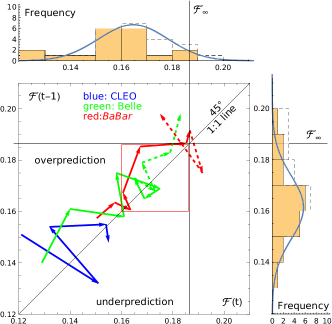
Figure 4: 2D projection in the phase space of the reconstructed attractors in terms of lagged coordinate vectors extracted from different data sets using for the basic series a constant sampling length, $\tau_{s}=1$ GeV². The assignment of the attractors to the data from bottom to top is as follows: CLEO (blue lines) Gronberg et al. (1998a), Belle (green lines) Uehara et al. (2012a), and BABAR (red lines) Aubert et al. (2009). The underlined time series $\mathcal{F}(t)$ (basic series), $\mathcal{F}(t-1)$ (lag-one series), and $\mathcal{F}(t-2)$ (lag-two series) are specified in the text. The shaded histograms count the frequency of the combined vector occurrences in each bin across the range of values common to all three attractors. Data values at the intersection of two bins, are placed in the next higher bin. The dashed lines signify additional vectors from data points measured at somewhat larger time intervals than $\tau_{s}$ (see the text). They are not included in the shaded histograms and in the distributions, but are taken into account in the histograms bounded by dashed lines. The red square shows the region bounded from above by the asymptotic TFF value $\mathcal{F}_{\infty}$ and adjusted to contain most vectors.

We begin by introducing the technique in terms of a discrete sampling of some generic experimental data set on the single dynamical variable $\mathcal{F}(Q^{2})$/GeV (omitting the dimension in the following discussion) and represent it as a time series of observations $\left(y(t_{1}),y(t_{2}),y(t_{3}),\ldots,y(t_{N_{s}})\right)$, where $N_{s}$ is the total number of samples in the set $s$. To construct a basic time series $\mathcal{F}(t_{i})$ we define a fixed sampling time $\tau_{s}=y(t_{i+1})-y(t_{i})=1$ GeV² and select a regular subseries of elements at equidistant time scales separated by $\tau_{s}=1$ GeV². The lag $\tau$ is the time difference between the time series we are correlating. For convenience, we define the lag time in terms of a parameter $J$ that counts the omitted elements within the delayed time series, $\tau=J\tau_{s}$. The basic time series corresponds to $J=0$, the one-lagged time series (one observation removed from the basic series) is obtained for $J=1$, the two-lagged series (offset from the basic series by two observations) for $J=2$ and so on, while the total number of observations in each lagged series is $N_{s}-J$. Then, the elements visible in the $(n,J)$-window Broomhead and King (1985) constitute the components of a vector in the embedding space $\mathbb{R}^{n}$ with the embedding dimension $n\geq 2m+1$ Takens (1981). To avoid false projections by embedding the system $\mathcal{F}$ in too few dimensions, we chose in this work $n=3$ that proves to be sufficient to unfold the structure of the attractor and enables at the same time its geometric visualization.

The choice of the time delay $\tau$ is arbitrary, but there are limitations, see, Pecora et al. (2007) and references cited therein. Adopting overly short lags, would induce strong correlations between the time-series we compare, causing the attractor to collapse on the $1:1$-line at 45^∘ in the embedding phase space, so that the delayed vectors cannot be resolved (almost linear regression). On the other hand, increasing significantly the delay would average out existing correlations between adjacent events but would eventually contain too little mutual information to reconstruct the attractor, making it impossible to discover any determinism inside the data (like in a random time series). The optimal delay choice should ensure the statistical independence of distant time-series neighbors maintaining at the same time the right amount of feedback to keep lagged events connected to each other. This renders the number of the state vectors sufficiently large in order to enable the attractor reconstruction, avoiding a featureless thus uninteresting portrait. Finally, if the number of events is small, like in our case, choosing a large lag $\tau>2$ would reduce the number of state vectors in the lagging process dramatically. This would obscure the tell-tale characteristics of the attractor considerably and reduce its usefulness.

Once the basic series $\mathcal{F}(t)$ for each data set has been selected, one can create additional time series with $N-J$ elements by displacing the time value and shifting the basic time series for its entire length by one unit ($J=1$), two units ($J=2$), etc. This way, a sequence of $n$ lagged coordinate vectors in the embedding space $\mathbb{R}^{n}$ can be generated: $\mathcal{F}(t-1)$ (lag-one series), $\mathcal{F}(t-2)$ (lag-two series) and so on, where we used the convenient notation $\mathcal{F}(t_{i}-J\tau)=\mathcal{F}(t-J)$ with $\tau=1$. The lagged vectors on the attractor form a discrete trajectory, i.e., a scatter plot in $\mathbb{R}^{n}$, given by the expression

$$\mathbf{X}_{i} = \Phi_{\mathbf{F},\mathbf{v}}\left(\varphi_{t}(\mathbf{y})\right)$$ (38)

$$= \left(v_{i},v_{i+J},v_{i+2J},v_{i+3J},\ldots,v_{i+(n-1)J}\right)^{\text{T}}\,.$$

Here $\mathbf{X}_{i}$ can be a column vector, representing a univariate time series with $N_{s}$ data points, or a trajectory matrix composed of a multivariate time series in terms of a sequence of $N=N_{s}-(n-1)$ vectors, $\{\mathbf{x}_{i}\in\mathbb{R}^{n}|i=1,2,\ldots N\}$ in the embedding space. The rows of the trajectory matrix correspond to events occurring at the same time, while each column denotes an individual time series. The oldest measurements on the system appear in the first row, whereas the most recent ones appear in the last row. In other words, applying the first lag to every series in $\mathbf{X}$, then the second lag to every series in $\mathbf{X}$, and so forth and so on, one obtains a sequence of lagged vectors to describe the whole evolution trajectory of the measured system.

All these properties can be expressed in terms of the following trajectory (or embedding) matrix

$$\mathbf{X}=N^{-1/2}\begin{bmatrix}x(t)&x(t-1)&x(t-2)&\dots&x(t-n)\\ x(t-1)&x(t-2)&x(t-3)&\dots&x(t-1-n)\\ x(t-2)&x(t-3)&x(t-4)&\ldots&x(t-2-n)\\ \vdots&\vdots&\vdots&\ddots&\vdots\\ x(t-N_{s})&x(t-N_{s}-1)&x(t-N_{s}-2)&\dots&x(t-N_{s}-n)\end{bmatrix}\,,$$ (39)

where $N^{-1/2}$ is a convenient normalization factor and $n$ is the embedding dimension. This $(N-n)\times(n+1)$ matrix contains the complete history of the measured dynamical system in the space of all $n$-element patterns in the embedding space $\mathbb{R}^{n}$ and can be considered as a linear map from $\mathbb{R}^{n}$ to $\mathbb{R}^{N}$ (see Broomhead and King (1985) for further discussion).

III.2 Attractor reconstruction

Let us now specify the above considerations by displaying the time series used in our TFF analysis. We construct the basic series for the CLEO measurement Gronberg et al. (1998a) from the data given in Table 2 by selecting events at $t=Q^{2}$ values in steps of approximately 1 GeV². This gives rise to the first column of the embedding matrix for CLEO (label C), viz.,

$$\mathcal{F}(t)^{\text{C}}=[0.121,0.151,0.132,0.154,0.155,0.148,0.167]^{T}\,.$$ (40)

Shifting this series by the first lag, we get the second column, i.e., the lag-one-series

$$\mathcal{F}(t-1)^{\text{C}}=[0.151,0.132,0.154,0.155,0.148,0.167]^{T}$$ (41)

and by shifting it by the second lag, we obtain the third column (the lag-two series)

$$\mathcal{F}(t-2)^{\text{C}}=[0.132,0.154,0.155,0.148,0.167]^{T}\,.$$ (42)

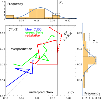
Figure 5: 2D projection of the reconstructed attractor in terms of lagged coordinate vectors with respect to $\mathcal{F}(t)$ and $\mathcal{F}(t-2)$. The same designations as in Fig. 4 are used.

We then construct the attractor portrait in terms of 3D vectors on the trajectory, denoted by the symbol $\bullet$, from the first five rows of these three columns in the form

$$\bullet=[\mathcal{F}(t),\mathcal{F}(t-1),\mathcal{F}(t-2)]\,,$$ (43)

while elements in the remaining rows are lost in the lagging process.

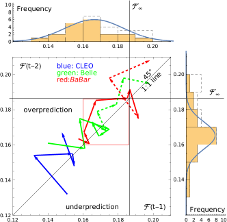
Figure 6: 2D projection of the reconstructed attractor in terms of lagged coordinate vectors with respect to $\mathcal{F}(t-1)$ and $\mathcal{F}(t-2)$. The same designations as in Fig. 4 are used.

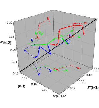
Figure 7: Attractor reconstruction in a 3D embedding phase space using the same time series as in the previous 2D plots related to three different sets of data and using the designations explained in Fig. 4. The dashed lines show the footprints of the two-dimensional projections displayed in Figs. 4, 5, and 6, while the additional vectors shown there by broken lines are not included. The black solid line marks the $1:1$ line at $45^{\circ}$.

The basic series from the BABAR (label B) Aubert et al. (2009) and the Belle (label b) Uehara et al. (2012a) data, displayed in Table 2, are assembled analogously to obtain

$$\mathcal{F}(t)^{\text{B}} \!\!\!\!\!\!=[0.150,0.157,0.164,0.161,0.167,0.185,$$

$$~{}0.187,\underline{0.192},\underline{0.175},\underline{0.198},\underline{0.208}]^{T}\,,$$

$$\mathcal{F}(t)^{\text{b}} \!\!\!\!\!\!=[0.129,0.140,0.161,0.158,0.175,0.169,$$

$$~{}0.165,\underline{0.173},\underline{0.168},\underline{0.179},\underline{0.183},\underline{0.198},\underline{0.195}]^{T}\,,$$

respectively. From these two basic series, we deduce the corresponding lag-one and lag-two series and then create from the BABAR data seven regular and two approximate 3D vectors, whereas from the Belle data we obtain seven regular 3D vectors and four approximate ones. The approximate vectors in each case have a sampling time $1<\tau_{s}<2.0$ GeV² and refer to the underlined numbers in the corresponding basic series. All data of both experiments above 15.95 GeV² (BABAR) and 22.24 GeV² (Belle) cannot be included in the corresponding basic series because they were measured at distant momentum values much larger than the sampling time $\tau_{s}=1$ GeV². Thus, they are excluded by the embedding procedure and not arbitrarily. Unfortunately, even the approximate vectors correspond to momenta below 20 GeV², notably, $Q^{2}=12.71$ GeV² (ninth BABAR vector) and $Q^{2}=16.96$ GeV² (eleventh Belle vector). Therefore, the measurements at momenta larger than these values, where one would expect a scaling behavior of the TFF starting to emerge, could not be taken into account in the considered attractor reconstruction. However, this is not a deficiency of the method but the consequence of sparse measurements in this $Q^{2}$ region.

The two-dimensional (2D) projections of the phase-space reconstruction are shown in Figs. 4, 5, 6 (with designations explained in the first of them). Each trajectory represents a separate phase portrait of the attractor related to a particular measurement of $\mathcal{F}(Q^{2})$ according to Eq. (38). A dashed lining is used for the approximate vectors to indicate that there are some missing jags along this trajectory owing to the fact that the sampling time is larger than $\tau_{s}=1$ GeV². In other words, the event collection in this part of the basic series entails a certain imprecision in the structure of the trajectory.

The scatter-plot emerging from the CLEO data is shown in blue color and starts close to the bottom and ends at the center. The BABAR trajectory (red lines) occurs at the center and extends to the far-end of the displayed time series, while the Belle trajectory (in green color) crosses the other two in between as it climbs. No experimental errors are included in these figures. For illustration, we combine these 2D projections of the considered time series into a 3D graphics shown in Fig. 7. Note that the approximate vectors are not included here. The broken lines denote instead the various 2D projections corresponding to Figs. 4, 5, 6.

From these figures we observe that the structure of the data attractors has been sufficiently resolved: not too smooth (ordered), not too jagged (disordered)—just right to recognize a deterministically generated pattern. This provides justification for the choice of the employed embedding parameters. Moreover, though the reconstructed attractors, emerging from each of these times series, show some idiosyncratic structure, they are composed of vectors clustering rather close to each other with a frequency peak in the range

$$\mathcal{F}(Q^{2})\in[0.16-0.17]~{}\text{GeV}\,,$$ (46)

occurring in the momentum region

$$Q^{2}\in[9-11]~{}\text{GeV}^{2}\,,$$ (47)

as quantified by the histograms. As one can see from Table 2, TFF values around this estimate have been measured by all three considered experiments in the momentum range $Q^{2}\in[6-10]$ GeV². Counting all 12 measurements in the range $[6.47-10.48]$ GeV², we get a statistical average of $\mathcal{F}\approx 0.167$ GeV in good agreement with the attractor value in the histograms. Including into the reconstruction procedure the displayed approximate vectors, the histograms are shifted closer to the asymptotic limit $\mathcal{F}_{\infty}$ so that the distributions become negatively skewed towards this value, while the estimated TFF value slightly increases. Ultimately, the geometry of the trajectory segments inside the asymptotic attractor area becomes irrelevant, because the system has reached an equilibrium state of its dynamics close to the fixed point $\mathcal{F}_{\infty}$ with the state vectors pointing in opposite directions at almost equal rates.

Based on this reasoning, we argue that the obtained attractor structure, cf. Eqs. (46), (47), where all particular trajectories have repetitive vector occurrences to neighboring states, represents a prodromal portrait of the true asymptotic attractor that would emerge if we would have at our disposal a finer partition of measurements in steps of 1 GeV² in the range between 10 GeV² and 25 GeV² to improve the convergence of the bootstrapping procedure to the correct limit. We estimate that to get a faithful attractor reconstruction, we need from a future experiment a series of TFF measurements starting, say, at 4.48 GeV² and continuing up to 25.48 GeV² in steps of 1 GeV². This way, we would obtain in total 20 3D state vectors for the attractor reconstruction. Assuming experimental errors similar to or smaller than those of the Belle measurements, this attractor portrait would suffice to establish the asymptotic limit of the TFF already below 25 GeV². That is to say, the attractor not only provides a shortcut to abbreviate the experimental efforts, it can also be used as a diagnostic tool to sort out events that contradict scaling above this momentum. On the other hand, if the described scenario will not be confirmed, the odds are stacked against the experimental observation of scaling in the TFF.

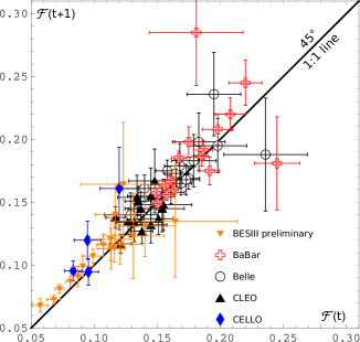
Figure 8: 2D attractor reconstruction from all existing data sets using each of them as a basic time series with varying sampling-time intervals. The state space reconstruction fails because the attractor remains hidden in the “width” of the data distribution along the $1:1$ line at $45^{\circ}$. Those data, which are compatible with an asymptotic scaling of the TFF, show a strong positive correlation, whereas the auxetic BABAR data above $\sim 10$ GeV² and the Belle outlier at 27.33 GeV² (see Table 2) are distributed according to a significant negative correlation.

We postpone further discussion of these figures to the next section and consider the possibility of applying the method of time delays to all data (CELLO, CLEO, BABAR, Belle, together with their experimental errors (see Table 2) using for each of them an unevenly sampled basic series from the recorded measurements as they appear in Table 2. We also include the BESIII preliminary data Redmer (2018) as they appear, i.e., with a varying sampling time $\tau_{s}$. We only consider the correlation of this ensemble of basic time series with the common “lagged-one” time series $\mathcal{F}(t-1)$, i.e., we fix the embedding dimension to $n=2$. The results are plotted in Fig. 8. Despite the application of an inaccurate phase-space reconstruction, resulting from the extremely short sampling times and varying lags, there are some striking observations from this figure. First, as expected, the attractor structure fails to unfold, with all state vectors being “buried” inside the (noisy) data width of the $1:1$ line showing in toto a positive correlation. This behavior agrees with the global trend of the attractors determined before using a strict embedding procedure. Second, the linear regression trend is especially accentuated in the case of the preliminary BESIII data at $Q^{2}$ values below 1.5 GeV², which are very close to each other and thus induce a strong autocorrelation. On the other hand, the large total error of these data at the upper end of $Q^{2}$ up to 3.1 GeV² does not allow to draw reliable conclusions. Third, in contrast to this overall trend of the entirety of the analyzed data, there is a segregated group of states forming a pattern, which, as a whole, exhibits a negative correlation. Interestingly, this pattern pertains exactly to those BABAR data points that deviate from the scaling limit of pQCD (see Fig. 2). The Belle outlier at $Q^{2}=27.33$ GeV² (see Table 2) also belongs to this group. These opposing tendencies of the system trajectories cannot be attributed to a common dynamical mechanism for the evolution of the measured system in its state space, pointing to an intrinsic incompatibility within the data. Remarkably, this inconsistency cannot be inferred from Fig. 2 in the statistical sense because, as shown in Uehara et al. (2012a); Stefanis et al. (2013), the relative deviation between the BABAR and Belle data fits does not exceed $1.5\sigma-2\sigma$.

IV LCSR predictions versus phase-space reconstruction

In this section we compare the TFF predictions obtained within QCD in Sec. II with the attractor phase portrait extracted from the data in the previous section. The strategy is to identify those particular features of the calculated TFF that provide agreement or disagreement with the determined attractor. To a great extent, this evaluation integrates and expands our previous analysis of the typical pion DAs considered in Table 1 and Figs. 2, 3.

To this end, let us first provide a brief quantitative assessment of the TFF calculation within our QCD-based LCSR approach. Using collinear factorization, the leading-twist part of the TFF at the NNLO of the perturbative expansion reads (see Sec. II for the explicit expressions)

$$F^{\gamma^{*}\gamma^{*}\pi^{0}}(Q^{2},q^{2})\! \!=\! \!N_{\text{T}}\Bigg{[}\underbrace{T_{\text{LO}}}_{(+)}+a_{s}(\mu^{2})\underbrace{T_{\text{NLO}}}_{(-)}+a^{2}_{s}(\mu^{2})\bigg{(}\underbrace{T_{{\rm NNLO}_{\beta_{0}}}}_{(-)}+\underbrace{T_{{\rm NNLO}_{\Delta V}}}_{(-)}+\underbrace{T_{{\rm NNLO}_{L}}}_{(0)}+\underbrace{T_{{\rm NNLO}_{c}}}_{(?)}\bigg{)}+\ldots\Bigg{]}\otimes\varphi_{\pi}^{(2)}(x,\mu^{2})$$

$$+\! \!\mathcal{O}\left(\frac{\delta^{2}}{Q^{4}}\right)$$ (48)

with indications showing the sign of these contributions. The label $(?)$ marks the only still uncalculated term. It is the source of the major theoretical uncertainties illustrated in Figs. 2 and 3 in terms of the wider blue shaded band enveloping the green one. The other NNLO contributions are included. Employing the LCSR formalism, we obtain the TFF for one highly virtual and one quasireal photon in the form

$$Q^{2}F^{\gamma*\gamma\pi^{0}}(Q^{2})=F^{\text{tw-2}}(Q^{2})+F^{\text{tw-4}}(Q^{2})+F^{\text{tw-6}}(Q^{2})\,,$$ (49)

where

$$F^{\text{tw-2}}(Q^{2})=F_{0}(Q^{2})+\sum_{n}a_{n}(Q^{2})F_{n}(Q^{2})\,.$$ (50)

Referring to the above equations, we now summarize the key ingredients of the LCSR analysis taking also into account relevant results from previous investigations.

• The Tw-4 term is negative, whereas the Tw-6 contribution is positive. Both are included explicitly as explained in Sec. II.

• NLO evolution with heavy-quark thresholds provides suppression that depends on the heavy-quark masses and the amount of the Gegenbauer coefficients included in the conformal expansion of the pion DA, see Sec. II and App. A.

• Consideration of a finite virtuality of the quasireal photon also leads to suppression Stefanis et al. (2013). This effect is not universal; it depends on the experimental set-up and is of minor importance for our present study. Therefore, it is not included.

• As a rule, DAs with suppressed tails $x=0,1$ tend to decrease the size of the TFF, while those with endpoint enhancement tend to increase it. For a quantitative treatment of these issues, we refer to Mikhailov et al. (2010); Stefanis et al. (1999, 2015); Stefanis and Pimikov (2016). In particular, the interplay between the “peakedness” of a DA at $x=0.5$ and the “flatness” or enhancement of its tails at $x=0,1$ can be quantified in terms of the kurtosis statistic $\beta_{2}[\varphi]=\langle\xi^{4}\rangle/\left(\langle\xi^{2}\rangle\right)^{2}$, see Stefanis and Pimikov (2016).

• The signs and magnitudes of the Gegenbauer coefficients also have a strong effect on the overall size of the TFF. This becomes evident by recalling Eq. (LABEL:eq:inv-mom) for the inverse moment. It implies that the Gegenbauer coefficients have to balance each other in such a way as to provide just the right amount of enhancement relative to the asymptotic DA. For example, the coefficients $a_{2}$ and $a_{4}$ of the BMS DA and the platykurtic DA have comparable magnitudes but opposite signs (see Table 1), whereas higher-order coefficients are marginal and contribute mainly to the theoretical uncertainties, so that the negative contributions mentioned in the previous items amount to a reduction of the total value of the TFF just to the gross size of the data, except the auxetic ones. There is a variation in the rate and extent of the influence of the Gegenbauer coefficients as one can see for some other DAs from Table 1 in comparison with Fig. 2.

• Among the considered pion DAs, the platykurtic model Stefanis (2014) has the following advantages: (i) It has only two conformal coefficients $a_{2}$ and $a_{4}$, with all higher coefficients being compatible with zero. This enables ERBL evolution at the two-loop level including heavy-quark thresholds (App. A). (ii) It amalgamates by construction endpoint suppression (via $\lambda_{q}^{2}=0.45$ GeV²) with unimodality (like in DCSB DAs). (iii) It gives $\varphi_{\pi}^{(2)\text{pk}}(x=0.5,\mu_{2})=1.33$ and thus satisfies the constraint $1.2\pm 0.3$ calculated with LCSRs in Braun and Filyanov (1989). (iv) It yields $\langle x^{-1}\rangle(\mu_{2})=3.13$ (Table 1), which is sufficient to accurately describe all data from low to high $Q^{2}$, provided the latter are compatible with scaling. (v) It resides inside the asymptotic regime of the determined attractor cf. Eqs. (46), (47), once it reaches the value $\mathcal{F}(Q^{2})=0.16$ around $Q^{2}\lesssim 11$ GeV². (vi) It complies within the margin of error with the new lattice results at NNLO and NLO Bali et al. (2019) for $a_{2}$ at $\mu_{2}$, keeping in mind that the NLO evolution procedure with heavy-quark thresholds induces a stronger reduction of the initial value (Table 1). All these features ensue from the applied construction procedure Stefanis and Pimikov (2016) and are not the product of a fit to any data.

• Best agreement with the BABAR auxetic data can be achieved by using flat-type DAs Radyushkin (2009); Polyakov (2009), though also DAs with an inverse hierarchy of several Gegenbauer coefficients, like model II in Agaev et al. (2011), may also provide conforming predictions. Flat-type DAs overestimate both, the CLEO and the Belle data (see Bakulev et al. (2012); Agaev et al. (2012)).

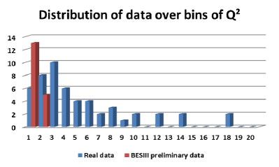
Figure 9: Histograms of assembled data from Table 2 in bins of $Q^{2}$ in the range between 0 and 40 GeV² (20 bins in total). The momentum increment between markers on the $x$ axis is 2 GeV². The $y$ axis shows the frequency, i.e., the total number of data points (blue color) in each bin by combining all available measurements (CELLO Behrend et al. (1991), CLEO Gronberg et al. (1998a), BABAR Uehara et al. (2012a), and Belle Aubert et al. (2009)). The preliminary data of BESIII Redmer (2018) below bin 3 are shown separately in red color. Only $35\%$ of the data occurs above bin 5, i.e., above 10 GeV².

We now turn our attention to the topology-based data analysis.

First, using for each of the CLEO, BABAR, and Belle data sets a basic time series with a sampling interval $\tau_{s}=1$ GeV², we reconstructed the state space of the TFF in terms of lagged coordinate vectors. More importantly, in Figs. 4, 5, 6, we identified and quantified in terms of histograms a common restrained region (red square) within this space, where the BABAR and Belle trajectories show both an aggregation of state vectors around the value $\mathcal{F}(Q^{2})=0.165\pm 0.005$ GeV that appears in the momentum range $Q^{2}\in[9-11]$ GeV². We argued that this attractor regime is a transient version of the true long-term attractor that would emerge closer to $\mathcal{F}_{\infty}$, if a more dense set of data between 10 and 25 GeV² would have been included in the analysis. This $Q^{2}$ range was inefficiently covered in all experiments so far.

This becomes evident from Fig. 9, where we show the experimental data, given in Table 2, plotted as a histogram across the values of $Q^{2}$ from 0 to 40 GeV². The bins show combined data of different experiments within successive intervals of 2 GeV² each numbered from 1 to 20, starting from the interval $1:[0-2]$ GeV² up to the interval $20:[38-40]$ GeV². There are in total 52 points composed as follows: CELLO (5), CLEO (15), BABAR (17), and Belle (15). For the sake of completion, the 18 preliminary data points of BESIII Redmer (2018) have also been included using a different color to distinguish them from final data published in peer-reviewed journals. As one observes from this figure, the data do not form a uniform distribution over $Q^{2}$. In fact, over 50 percent of the events occur below bin $5:[10-12]$ GeV². The $Q^{2}$ intervals above 20 GeV² are only scarcely populated and some of the data in this high-end $Q^{2}$ regime bear rather large errors (see Table 2 and Fig. 2).

Second, from the approximate embedding procedure shown in Fig. 8, we observed a conflicting behavior of the data concerning the states of the TFF in its phase space. While most data points, encompassing the preliminary BESIII, CELLO, CLEO, Belle, and BABAR below 10 GeV², describe TFF states that follow in round terms a positive correlation pattern along the diagonal, the high-end BABAR data together with the Belle event at 27.33 GeV² are found to be negatively correlated. Data from new experiments may contribute to the clarification of this observed discrepancy. In this context, we mention that this observation is in line with the statistical analysis carried out in Stefanis et al. (2013) in which we investigated the possibility to predict the trend of the Belle and the BABAR data from one another. We found that both popular parametrizations, a dipole and a power-law function can fit the Belle data in a satisfactory way, while only the power fit works well for the BABAR data. However, using the corresponding parameters of these fit functions, determined for each of these sets, one cannot reproduce the other with an acceptable statistical precision. The inclusion of the CELLO and CLEO data into this fitting procedure does not modify this finding. The conclusion drawn in Stefanis et al. (2013) was that the Belle and BABAR data segregate into two separate classes that cannot be fitted simultaneously.

Third, from Table 2, we observe that the TFF value calculated with the BMS DA (or equivalently the platykurtic one) does not change appreciably after $Q^{2}=10.48$ GeV², where it reaches the value 0.161 GeV. This implies that the corresponding phase-space trajectory will enter at this scale the red square determined in Figs. 4, 5, 6 and then stay within it, merging practically with the diagonal after some point. Thus, this TFF prediction agrees with the existence of the reconstructed attractor and supports a saturating behavior of the TFF starting around [9-11] GeV². On the other hand, TFF predictions that exceed the asymptotic limit within the range of the available data, e.g., the result obtained with the DSE-DB DA, will give rise to phase-space trajectories following the direction of the diagonal after exiting the attractor portrait (the red square) and continuing to grow slowly at some variable distance from it. In fact, the histograms in that case are approximately uniform with no distinctive maximum at some value. Finally, TFF predictions that are tailored to reproduce the auxetic BABAR data in terms of a flat pion DA, will cross the attractor residence within the red square and then diverge from it towards increasingly larger values along jagged trajectories. This just reflects the feature that the fluctuations away from the diagonal can be much larger than the average direction of the evolution trajectory on the attractor. Consequently, such predictions are not compatible with the existence of an attractor within the TFF data showing up in the range $[9-11]$ GeV² and, therefore, they contradict the onset of QCD scaling in this $Q^{2}$ domain.

V Conclusions

This section summarizes the benchmarks of our analysis and presents our conclusions.

In this work we scrutinized the single-tagged process $e^{+}e^{-}\rightarrow e^{+}e^{-}\pi^{0}$ in terms of the pion-photon transition form factor $\gamma^{*}\gamma\rightarrow\pi^{0}$, described by the quantity $F^{\gamma^{*}\gamma\pi^{0}}(Q^{2})$. Observations of this exclusive process can provide insight into the dynamical characteristics of the electromagnetic $\pi^{0}$ vertex and its microscopic explanation at the quark-gluon level using particular theoretical formalisms or models. To obtain reliable predictions and include their intrinsic uncertainties, we employed a LCSR-based scheme which is embedded into the collinear factorization framework of QCD and the twist expansion. This dispersive approach allows the systematic inclusion into the spectral density of perturbative radiative corrections together with the contributions from higher twists. Moreover, the obtained expression for the TFF retains its validity also in the case of a quasireal photon emitted from the untagged electron. The approach can be used with various pion DAs in terms of their conformal expansions, thus facilitating the inclusion of ERBL evolution.

In the presented analysis, we included perturbative contributions to the hard-scattering amplitude up to the NNLO, except a single term which is still unknown, see (18). The used spectral density also includes the twist-four and twist-six corrections. In our predictions the binding effects of the pion were taken into account in the form of various pion DAs. We used two twist-two DAs derived with QCD sum rules employing nonlocal condensates Mikhailov and Radyushkin (1986a). One family of DAs has a bimodal profile and suppressed tails at $x=0,1$ Bakulev et al. (2001) ($\lambda_{q}^{2}=0.4$ GeV²). Allowing for a slightly larger (but still admissible) average vacuum quark virtuality $\lambda_{q}^{2}=0.45$ GeV², one can obtain a DA with a short-tailed platykurtic profile Stefanis (2014). The TFF computed with these DAs at the momentum values probed experimentally are given in Table 2 together with the chief theoretical uncertainties discussed in Sec. II.

To obtain a variety of TFF predictions, we also employed pion DAs obtained in other approaches, for instance, the DAs with enhanced endpoint regions from DSE-based calculations Chang et al. (2013); Raya et al. (2016) or AdS/QCD Brodsky et al. (2011b). Predictions from some other models have also been included, see Fig. 2. To connect the calculated TFF predictions at the initial scale (either $\mu_{1}=1$ GeV or $\mu_{2}=2$ GeV) to the measurements at higher momentum scales, we employed NLO evolution that contains an arbitrary number of conformal coefficients and takes into account heavy-quark thresholds (see App. A). The statistical measures to quantify the interplay of the “peakedness” (in terms of the second moment or $a_{2}$) and the “tailedness” (by means of the fourth moment or $a_{4}$) of these DAs were discussed in connection with Table 1.

To analyze the asymptotics of the TFF predictions, we invented and used a new quantity which measures the deviation of the TFF value from the asymptotic limit set by pQCD, see Eq. (36) and Fig. 3. The upshot of these considerations can be encapsulated in the following statement. Pion DAs with enhanced tails tend to increase the magnitude of the TFF to a level above the asymptotic limit $\mathcal{F}_{\infty}=\sqrt{2}f_{\pi}$, while the considered DAs with suppressed endpoint regions $x=0,1$ yield predictions that approach this limit from below without crossing it. Both types of predictions are, therefore, compatible with the scaling property of pQCD at asymptotic momentum scales and therefore disagree with the auxetic BABAR data points above 10 GeV². We didn’t discuss model calculations attempting to explain this data behavior and refer to our previous dedicated analysis in Bakulev et al. (2012) and references cited therein.

The QCD-based calculations were supplemented by a topology-based data analysis, carried out in Sec. III. We showed that topological embedding subject to Taken’s theorem provides a mathematical scaffolding to carry out a nonlinear time-series analysis of the observed TFF data to unveil the underlying dynamics without appealing to any theoretical formalism or model. The key components of the method to reconstruct the state space of the system (the TFF) were described and the embedding matrix for the delayed time series vectors was worked out. The intrinsic and practical limitations of the method were also pointed out. Using appropriate embedding parameters, we determined the phase portrait of two attractors in 3D space, one related to the data of the Belle experiment and the other pertaining to BABAR. The controversial branch of the auxetic BABAR data above 10 GeV² was excluded by the applied embedding parameters—not arbitrarily. Nevertheless, both attractor structures enter a common area of phase space, where they have a maximum of state vector occurrences around the value $\mathcal{F}(Q^{2})=0.165\pm 0.005$ GeV emerging at scales in the range $Q^{2}\in[9-11]$ GeV² and marking the onset of asymptotic scaling. This dynamical characteristic was quantified in terms of histograms in Figs. 4, 5, 6. We argued that this generic attractor portrait provides a shadowing reflection of the true asymptotic attractor to be determined from future experiments, e.g., Belle-II. We claimed that the final arrangement of the data-driven state vectors can be revealed by the outcome of measurements from $Q^{2}=10.48$ GeV² to $Q^{2}=25.48$ GeV² (like in the Belle experiment) with a fixed increment of 1 GeV². We encourage the Belle-II Collaboration to design the data acquisition of their experiment accordingly.

Understanding the phase-space structure of the data on the pion-photon transition would be an essential step towards determining the asymptotic behavior of the TFF that follows from the basic principles of QCD. We have shown that endpoint-suppressed pion DAs yield predictions which enter the attractor regime and then remain inside it. By contrast, TFF predictions derived with endpoint-enhanced DAs cross the asymptotic attractor area and then leave it again towards larger TFF values. Thus, a validated and accurate phase-state portrait of the attractor will provide a reliable diagnostic tool to select the most appropriate type of the pion DA. Combining it with the new more reliable lattice results of the RQCD Collaboration Bali et al. (2019) for the second conformal coefficient $a_{2}$, can reduce the variation of the DA profile even further (see the previous section). To this end, the determination of $a_{4}$ would be extremely useful but difficult to realize on the lattice Bali et al. (2019). In this sense, the attractor represents from the experimental side, a shortcut because it provides the possibility to establish the asymptotic structure of the TFF attractor and the observation of QCD scaling at much lower momentum values than anticipated until now, thus avoiding overemphasis of solitary data points with unconfirmed accuracy at much higher $Q^{2}$. Implicit in this statement is the optimistic perspective that the asymptotic regime of the TFF can be reached in a momentum range accessible to experiments. The outlined methodology provides the conceptual tools to obtain tangible results in this direction.

Appendix A NLO evolution of the pion DA with an arbitrary number of Gegenbauer harmonics and including heavy-quark thresholds

In this Appendix (done in collaboration with S. V. Mikhailov and A. V. Pimikov) we discuss the NLO (i.e., two-loop) ERBL evolution of the pion DA with an arbitrary number of Gegenbauer coefficients and taking into account heavy-quark flavors (also known as global QCD scheme, see, e.g., Bakulev and Khandramai (2013)). This scheme employs the global coupling $\alpha_{s}^{\text{glob}}(Q^{2},\Lambda_{N_{f}}^{2})$ that depends on the number of flavors $N_{f}$ through the QCD scale parameter $\Lambda_{N_{f}}$.

This procedure was used in this work to derive the results given in Tables 1 and 2 and obtain the predictions shown in Figs. 2 and 3. It takes into account the heavy-quark thresholds and thus requires the matching of the strong coupling in the Euclidean region of $Q^{2}$ at the corresponding heavy-quark masses when one goes from $N_{f}\to N_{f}+1$. Note that the dependence on $N_{f}$ in Appendix D of Bakulev et al. (2003), which provided the basis for the NLO evolution of the pion DA in our earlier works, was ignored assuming a fixed number of flavors. The new scheme has already been used in our more recent investigations Bakulev et al. (2012); Stefanis et al. (2013, 2015); Mikhailov et al. (2016), but without exposing the underlying formalism. This task will be accomplished here. The NLO evolution of the pion DAs with two conformal coefficients $a_{2}$ and $a_{4}$ at the initial scale $\mu^{2}\simeq 1$ GeV² and a varying number of heavy flavors has also been applied in Bakulev et al. (2004b) (see Appendix D there). Our technical exposition below extends this treatment to any number of conformal coefficients and more heavy-flavor thresholds, see Bakulev (2009); Bakulev and Khandramai (2013) for details and further references.

Let us start with a fixed number of flavors and supply some basic formulas from Bakulev et al. (2003). The ERBL evolution equation for the pion DA is given by

$$\frac{d\,\varphi_{\pi}(x;\mu^{2})}{d\,\ln\mu^{2}}=V\left(x,u;a_{s}(\mu^{2})\right)\underset{u}{\otimes}\varphi_{\pi}(u;\mu^{2})$$ (51)

and is driven by the kernel

$$V(x,y;a_{s})=a_{s}~{}V_{0}(x,y)+a_{s}^{2}~{}V_{1}(x,y)+\ldots$$ (52)

with $a_{s}=\alpha_{s}/(4\pi)$.

The eigenvalues $\gamma_{n}(a_{s})$ and the one-loop eigenfunctions $\psi_{n}(u)$ are related to the kernel $V$ through

$$\tilde{\psi}_{n}(x)\underset{x}{\otimes}V(x,u;a_{s})\underset{u}{\otimes}\psi_{n}(u)=-\gamma_{n}(a_{s})\,,$$ (53)

where $\displaystyle\tilde{\psi}_{n}(x)=2(2n+3)/\left[3(n+1)(n+2)\right]C^{3/2}_{n}(x-\bar{x})$. The explicit expressions for the anomalous dimensions $\gamma_{n}$ at one loop, $\gamma_{0}(n)$, and two-loops, $\gamma_{1}(n)$, in the expansion $\gamma_{n}(a_{s})=\frac{1}{2}[a_{s}\gamma_{0}(n)+a_{s}^{2}\gamma_{1}(n)+\ldots]$ can be found in Appendix D in Bakulev et al. (2003).

To perform the pion DA evolution, while ignoring quark-mass thresholds, we make use of the evolution matrix $E$ with the components $E_{nk}$. Expanded over the basis $\{\psi_{n}\}$ of the Gegenbauer harmonics, this matrix assumes the following triangular form Mikhailov and Radyushkin (1986b)

$$E_{nk}(N_{f};Q^{2},\mu^{2}) = P(n,Q^{2},\mu^{2})\left[\delta_{nk}+a_{s}(Q^{2})\Theta(k-n>0)d_{nk}(Q^{2},\mu^{2})\right]\,,$$ (54)

$$d_{nk}(\mu^{2},\mu^{2})=0\,,$$ (55)

where the coefficients $d_{nk}(Q^{2},\mu^{2})$ will be defined shortly, and where $\mu^{2}$ and $Q^{2}$ refer to the initial and observation scale, respectively. The factor $P(n,Q^{2},\mu^{2})$ in Eq. (54) denotes the diagonal part of the evolution matrix that dominates the renormalization-group (RG) controlled evolution of the $\psi_{n}$-harmonics in the conformal expansion

$$\varphi_{\pi}^{\text{RG}}(x,Q^{2}) = \sum\limits_{n}a_{n}(\mu^{2})\left\{P(n,Q^{2},\mu^{2})\left[\psi_{n}(x)+a_{s}(Q^{2})\sum\limits_{k>n}d_{nk}(Q^{2},\mu^{2})\psi_{k}(x)\right]\right\}\,.$$ (56)

Then, the diagonal part of the evolution exponential at the two-loop level can be given explicitly,

$$P(n,Q^{2},\mu^{2}) = \exp\left[\int\limits_{a_{s}(\mu^{2})}^{a_{s}(Q^{2})}\frac{\gamma_{n}(a)}{\beta(a)}da\right]\stackrel{{\scriptstyle 2-\text{loops}}}{{\longrightarrow}}\left[\frac{a_{s}(Q^{2})}{a_{s}(\mu^{2})}\right]^{\frac{\gamma_{0}(n)}{2b_{0}}}\left[\frac{1+c_{1}a_{s}(Q^{2})}{1+c_{1}a_{s}(\mu^{2})}\right]^{\omega(n)}\,,$$ (57)

where $a_{s}(\mu^{2})=\alpha_{s}^{\text{glob};(2)}(\mu^{2},\Lambda_{3}^{2})/(4\pi)$ and $c_{1}=b_{1}/b_{0}$, with $b_{i}$ being the expansion coefficients of the QCD $\beta$-function. The evolution exponent of the coupling is defined by $\omega(n)=[\gamma_{1}(n)b_{0}-\gamma_{0}(n)b_{1}]/[2b_{0}b_{1}]$. The second term in the brackets in Eq. (54) represents the non-diagonal part of the evolution equation to the order $O(a_{s}^{2})$ induced by renormalization and encodes the mixing of the higher Gegenbauer harmonics for indices $k>n$ related to the conformal-symmetry breaking at NLO Müller (1995). Notice that all components on the right-hand side of Eqs. (54) and (57) depend on $N_{f}$, which changes to $N_{f}+1$, when the next quark-mass threshold is crossed. The explicit form of the mixing coefficients is given by Bakulev et al. (2003)

$$d_{nk}(Q^{2},\mu^{2}) = \frac{M_{nk}}{\gamma_{0}(k)-\gamma_{0}(n)-2b_{0}}\left\{1-\left[\frac{a_{s}(Q^{2})}{a_{s}(\mu^{2})}\right]^{[\gamma_{0}(k)-\gamma_{0}(n)]/(2b_{0})-1}\right\}\,,$$ (58)

where the values of the first few elements of the matrix $M_{nk}$ ($k=2,4\geq n=0,2$) read

$$M_{02}=-11.2+1.73N_{f},~{}~{}M_{04}=-1.41+0.565N_{f},~{}~{}M_{24}=-22.0+1.65N_{f}\,.$$ (59)

Analytic expressions for $M_{nk}$ have been obtained in Müller (1994). The values in Eq. (59) reproduce the exact results with a deviation less than about $1\%$.

To make our further exposition more compact, we make use of the parameter vectors $\mathbf{A}(\mu^{2})$ and $\bm{\Psi}(x)$ defined at the reference momentum scale $\mu^{2}$ as follows

$$\mathbf{A} = (1,\,a_{2},\,a_{4}\,,\cdots,\,a_{2(N-1)})\,,$$ (60a)

$$\bm{\Psi} = (\psi_{0},\psi_{2},\cdots,\psi_{2(N-1)})\,,$$ (60b)

$$\varphi_{\pi}(x,\mu^{2}) = \sum\limits_{n=0}^{N-1}a_{2n}(\mu^{2})\psi_{2n}(x)$$ (60c)

$$= \mathbf{A}(\mu^{2})\bm{\Psi}(x)\,,$$

where their dimension and the dimension of the matrix $E$ depends on the parameter $N$. Then, the evolution of the pion DA can be carried out in terms of the Gegenbauer coefficients $a_{i}$ with $i=2,4,\ldots,2(N-1)$. For a fixed number of flavors, one gets

$$\bm{\Psi}(x;\mu^{2}) = E(N_{f},\mu^{2},\mu^{2}_{0})\bm{\Psi}(x),$$ (61a)

$$\mathbf{A}(\mu^{2}) = E^{\text{T}}(N_{f},\mu^{2},\mu^{2}_{0})\mathbf{A}(\mu_{0}^{2})\,,$$ (61b)

where $E^{\text{T}}$ is the transposed matrix of $E$, while $\mathbf{A}(\mu_{0}^{2})$ is the vector of the Gegenbauer coefficients defined at some initial scale $\mu_{0}^{2}$.

In the global QCD scheme, the evolution of the pion DA defined at the initial scale $\mu_{0}^{2}$, is implemented by means of the threshold interval factors $E_{i}$ in the following step-by-step procedure,

$$E_{\text{glob}}(\mu^{2},\mu^{2}_{0}) = E_{3}(\mu^{2})\theta(\mu^{2}<M_{4}^{2})+E_{4}(\mu^{2})\theta(M_{4}^{2}\leqslant\mu^{2}<M_{5}^{2})E_{3}+$$ (62)

$$E_{5}(\mu^{2})\theta(M_{5}^{2}\leqslant\mu^{2}<M_{6}^{2})E_{4}E_{3}+E_{6}(\mu^{2})\theta(M_{6}^{2}\leqslant\mu^{2})E_{5}E_{4}E_{3}\,,$$

where the matrices $E_{i}$ and $E_{i}(\mu^{2})$ are given by

$$E_{i}(\mu^{2})\equiv E(i,\mu^{2},M^{2}_{i})\,,~{}~{}E_{i}\equiv E(i,M^{2}_{i+1},M^{2}_{i})$$ (63)

and the thresholds are defined Bakulev and Khandramai (2013) by the heavy-quark masses $m_{c}\sim M_{4}=1.65$ GeV, $m_{b}\sim M_{5}=4.75$ GeV, and $m_{t}\sim M_{6}=172.5$ , while $M^{2}_{3}\equiv\mu^{2}_{0}$ sets the initial scale taken to be either $\mu_{0}=\mu_{1}=1$ GeV or $\mu_{0}=\mu_{2}=2$ GeV, see Table 1. Note that the global evolution matrix, Eq. (62), is presented for $\mu_{0}<M_{4}$ and $\mu>\mu_{0}$. No matching at the mass thresholds is needed in the case of equal initial and final momentum scales, i.e., $E(N_{f};Q^{2},Q^{2})=1$ because of the independence of the evolution matrix on the number of flavors. For example, at the threshold $M_{4}$, we have $E_{4}(M_{4}^{2})=1$ ensuring the continuity of the global evolution matrix $E_{\text{glob}}$. It is worth noting that our NLO evolution scheme in terms of Eq. (62), has the following improvements relative to that used in Bakulev et al. (2004b) (see Appendix D there): (a) It is applicable to DAs with any number of Gegenbauer harmonics. (b) The number of heavy-quark thresholds is extended to four flavors. (c) When the interval of evolution contains two or more thresholds, our method can still incorporate contributions from the non-diagonal part of the evolution matrix removing the restriction to use only the first two Gegenbauer coefficients $a_{2}$ and $a_{4}$ as in Bakulev et al. (2004b).

We reiterate that the matching of the coupling constants at the quark-mass thresholds requires the readjustment of the value of the QCD scale parameter $\Lambda$ to $\Lambda_{(N_{f})}$. A detailed description of the matching procedure of the running coupling in the global scheme can be found in Bakulev and Khandramai (2013) and references cited therein. For definiteness, we quote here the two-loop $\Lambda_{(N_{f})}^{(2)}$ values used in our code: $\Lambda_{(3)}^{(2)}=369$ MeV, $\Lambda_{(4)}^{(2)}=305$ MeV, $\Lambda_{(5)}^{(2)}=211$ MeV, $\Lambda_{(6)}^{(2)}=88$ MeV. These values are defined by fixing the strong coupling

$$\alpha_{S}(M_{Z}^{2})=0.118$$ (64)

at the scale of the Z boson mass $M_{Z}=91$ GeV.

We emphasize that for self-consistency reasons, the global two-loop coupling $\alpha_{s}^{\text{glob};(2)}(\mu^{2},\Lambda_{3})/(4\pi)$ should be used in all functions entering Eq. (54) that depend on the coupling with a variable flavor number $N_{f}$. Finally, the global evolution of the Gegenbauer coefficients is given by

$$\mathbf{A}_{\text{glob}}(\mu^{2})=E^{\text{T}}_{\text{glob}}(\mu^{2},\mu^{2}_{0})\mathbf{A}(\mu_{0}^{2})\,,$$ (65)

whereas the global evolution of the pion DA assumes the form

$$\varphi_{\pi}^{\text{glob}}(x,\mu^{2}) = \mathbf{A}_{\text{glob}}(\mu^{2})\bm{\Psi}(x)=\bm{A}(\mu_{0}^{2})\bm{\Psi}(x;\mu^{2})=\sum\limits_{n=0}^{N-1}a_{2n}^{\text{glob}}(\mu^{2})\psi_{2n}(x)\,.$$ (66)

Appendix B Data collection versus theoretical predictions

In this appendix, we collect in Table 2 all existing sets of experimental data on the pion-photon transition form factor together with our theoretical predictions. The results obtained with the BMS pion DA Bakulev et al. (2001) differ from those we reported before in Bakulev et al. (2011). The differences originate from the fact that we are using here an updated theoretical framework; see the text for explanations and Mikhailov et al. (2016) for details. In addition, we use the evolution scheme described in the previous Appendix. The numbers given in parentheses are new predictions calculated with the platykurtic pion DA determined in Stefanis (2014). The displayed theoretical uncertainties for the BMS set of pion DAs greatly overlap with those related to the platykurtic ones. Therefore, no error bars for the latter have been displayed.

Table 2: Compilation of all existing data on the scaled TFF $\tilde{Q}^{2}F^{\gamma^{*}\gamma\pi^{0}}(\tilde{Q}^{2})\equiv\mathcal{F}_{\gamma\pi}(\tilde{Q}^{2})$ from different measurements: (i) CELLO Behrend et al. (1991), (ii) CLEO Gronberg et al. (1998a), (iii) BABAR Aubert et al. (2009), and (iv) Belle Uehara et al. (2012a). The TFF is measured at $\tilde{Q}^{2}$ where the differential cross sections assume their mean values computed by numerical integration. The last column shows the theoretical predictions calculated in this work at the same momentum value $\tilde{Q}^{2}$ for each bin using as nonperturbative input the bimodal BMS pion DA Bakulev et al. (2001) and taking into account the chief theoretical uncertainties as explained in Sec. II. The numbers in parentheses show the results obtained with the platykurtic (pk) pion DA Stefanis (2014) bearing uncertainties inside the previous ones. Both types of DAs have suppressed endpoint regions $x=0,1$ (see the text). NLO evolution, starting at $\mu_{1}=1$ GeV (Table 1), and including heavy-quark thresholds is employed, see App. A.

$Q^{2}$ bin range	$\tilde{Q}^{2}$	$\mathcal{F}_{\text{CELLO}}^{\gamma^{*}\gamma\pi^{0}}(\tilde{Q}^{2})$	$\mathcal{F}_{\text{CLEO}}^{\gamma^{*}\gamma\pi^{0}}(\tilde{Q}^{2})$	$\mathcal{F}_{\text{BABAR}}^{\gamma^{*}\gamma\pi^{0}}(\tilde{Q}^{2})$	$\mathcal{F}_{\text{Belle}}^{\gamma^{*}\gamma\pi^{0}}(\tilde{Q}^{2})$	$\mathcal{F}_{\rm BMS(pk)}^{\gamma^{*}\gamma\pi^{0}}(\tilde{Q}^{2})$
. [GeV2]	[GeV2]	[0.01 $\times$ GeV]	[0.01 $\times$ GeV]	[0.01 $\times$ GeV]	[0.01 $\times$ GeV]	[0.01 $\times$ GeV]
0.5 – 0.8	0.68	8.37${}_{-0.73}^{+0.67}$	–	–	–	5.39${}_{-3.37}^{+3.46}$(5.98)
0.8 – 1.1	0.94	9.58${}_{-0.84}^{+0.78}$	–	–	–	7.70${}_{-2.80}^{+2.90}$(7.95)
1.1 – 1.5	1.26	9.54${}_{-1.12}^{+1.00}$	–	–	–	9.94${}_{-2.50}^{+2.62}$(9.65)
1.5 – 1.8	1.64	–	12.1$\pm\,0.8\,\pm\,$0.3	–	–	11.78${}_{-2.46}^{+2.6}$(11.05)
1.5 – 2.1	1.70	12.08${}_{-1.62}^{+1.43}$	–	–	–	12.00${}_{-2.45}^{+2.59}$(11.23)
1.8 – 2.0	1.90	–	11.7$\pm\,0.7\,\pm\,$0.3	–	–	12.66${}_{-2.39}^{+2.55}$(11.75)
2.0 – 2.2	2.10	–	13.8$\pm\,0.8\,\pm\,$0.3	–	–	13.18${}_{-2.32}^{+2.49}$(12.19)
2.1 – 2.7	2.17	16.43${}_{-3.60}^{+2.94}$	–	–	–	13.33${}_{-2.29}^{+2.46}$(12.33)
2.2 – 2.4	2.30	–	12.7$\pm\,0.9\,\pm\,$0.3	–	–	13.59${}_{-2.24}^{+2.42}$(12.56)
2.4 – 2.6	2.50	–	13.5$\pm\,1.0\,\pm\,$0.3	–	–	13.93${}_{-2.16}^{+2.34}$(12.88)
2.6 – 2.8	2.70	–	15.1$\pm\,1.1\,\pm\,$0.4	–	–	14.20${}_{-2.07}^{+2.25}$(13.16)
2.8 – 3.1	2.94	–	13.7$\pm\,1.2\,\pm\,$0.3	–	–	14.46${}_{-2.01}^{+2.18}$(13.43)
3.1 – 3.5	3.29	–	14.5$\pm\,1.2\,\pm\,$0.4	–	–	14.75${}_{-1.93}^{+2.09}$(13.76)
3.5 – 4.0	3.74	–	13.2$\pm\,1.4\,\pm\,$0.3	–	–	15.01${}_{-1.84}^{+1.99}$(14.10)
4.0 – 4.5	4.24	–	13.4$\pm\,1.5\,\pm\,$0.3	15.04$\pm\,0.39$	–	15.21${}_{-1.76}^{+1.88}$(14.39)
4.0 – 5.0	4.46	–	–	–	12.9$\pm\,2.0\,\pm\,$0.6	15.28${}_{-1.72}^{+1.84}$(14.50)
4.5 – 5.0	4.74	–	15.4$\pm\,1.7\,\pm\,$0.4	14.91$\pm\,0.41$	–	15.36${}_{-1.68}^{+1.79}$(14.62)
5.0 – 5.5	5.24	–	14.5$\pm\,1.8\,\pm\,$0.4	15.74$\pm\,0.39$	–	15.48${}_{-1.61}^{+1.71}$(14.81)
5.0 – 6.0	5.47	–	–	–	14.0$\pm\,1.6\,\pm\,$0.7	15.52${}_{-1.58}^{+1.68}$(14.89)
5.5 – 6.0	5.74	–	15.5$\pm\,2.2\,\pm\,$0.4	15.60$\pm\,0.45$	–	15.57${}_{-1.55}^{+1.64}$(14.97)
6.0 – 7.0	6.47	–	14.8$\pm\,2.0\,\pm\,$0.4	16.35$\pm\,0.36$	16.1$\pm\,0.7\,\pm\,$0.8	15.68${}_{-1.48}^{+1.56}$(15.15)
7.0 – 8.0	7.47	–	–	16.06$\pm\,0.47$	15.8$\pm\,0.6\,\pm\,$0.7	15.80${}_{-1.40}^{+1.47}$(15.35)
7.0 – 9.0	7.90	–	16.7$\pm\,2.5\,\pm\,$0.4	–	–	15.84${}_{-1.37}^{+1.44}$(15.42)
8.0 – 9.0	8.48	–	–	16.73$\pm\,0.60$	17.5$\pm\,0.5\,\pm\,$0.7	15.89${}_{-1.34}^{+1.39}$(15.51)
9.0 – 10.0	9.48	–	–	18.53$\pm\,0.55$	16.9$\pm\,0.5\,\pm\,$0.7	15.97${}_{-1.28}^{+1.33}$(15.63)
10.0 – 11.0	10.48	–	–	18.66$\pm\,0.76$	16.5$\pm\,0.6\,\pm\,$0.7	16.04${}_{-1.24}^{+1.28}$(15.73)
11.0 – 12.0	11.48	–	–	–	17.3$\pm\,0.8\,\pm\,$0.7	16.10${}_{-1.20}^{+1.24}$(15.82)
11.0 – 12.0	11.49	–	–	19.16$\pm\,0.78$	–	16.10${}_{-1.20}^{+1.24}$(15.82)
12.0 – 13.5	12.71	–	–	17.50$\pm\,1.10$	–	16.16${}_{-1.16}^{+1.19}$(15.91)
12.0 – 14.0	12.94	–	–	–	16.8$\pm\,0.7\,\pm\,$1.0	16.18${}_{-1.15}^{+1.18}$(15.93)
13.5 – 15.0	14.22	–	–	19.80$\pm\,1.20$	–	16.23${}_{-1.12}^{+1.14}$(16.00)
14.0 – 16.0	14.95	–	–	–	17.9$\pm\,1.2\,\pm\,$1.3	16.26${}_{-1.10}^{+1.12}$(16.04)
15.0 – 17.0	15.95	–	–	20.80$\pm\,1.20$	–	16.30${}_{-1.08}^{+1.10}$(16.09)
16.0 – 18.0	16.96	–	–	–	18.3$\pm\,1.7\,\pm\,$1.2	16.33${}_{-1.06}^{+1.08}$(16.13)
17.0 – 20.0	18.40	–	–	22.00$\pm\,1.30$	–	16.38${}_{-1.03}^{+1.05}$(16.18)
18.0 – 20.0	18.96	–	–	–	19.8$\pm\,1.9\,\pm\,$1.3	16.39${}_{-1.02}^{+1.04}$(16.20)
20.0 – 25.0	22.28	–	–	24.50$\pm\,1.80$	–	16.47${}_{-0.97}^{+0.98}$(16.30)
20.0 – 25.0	22.29	–	–	–	19.5$\pm\,1.7\,\pm\,$1.3	16.47${}_{-0.97}^{+0.98}$(16.30)
25.0 – 30.0	27.31	–	–	18.10${}_{-4.0}^{+3.3}$	–	16.56${}_{-0.92}^{+0.93}$(16.40)
25.0 – 30.0	27.33	–	–	–	23.6${}_{-2.9}^{+2.6}$$\pm\,$1.6	16.56${}_{-0.92}^{+0.93}$(16.40)
30.0 – 40.0	34.36	–	–	28.50${}_{-4.5}^{+3.9}$	–	16.64${}_{-0.87}^{+0.87}$(16.49)
30.0 – 40.0	34.46	–	–	–	18.8${}_{-4.3}^{+3.5}$$\pm\,$1.3	16.64${}_{-0.87}^{+0.87}$(16.50)

It is instructive to make some important remarks concerning the CELLO data reported in Behrend et al. (1991). These data were presented for the quantity $\frac{F^{2}M^{3}}{64\pi}~{}\text{eV}\equiv a$, evaluated at the reference momentum scale $\langle Q^{2}\rangle\equiv\tilde{Q}^{2}$. They have been converted here to the quantity $Q^{2}F(Q^{2})$ using the relation $Q^{2}|F^{\gamma^{*}\gamma\pi^{0}}(\tilde{Q}^{2})|=\frac{1}{4\pi\alpha}\sqrt{\frac{64\pi a}{M^{3}}}|Q^{2}|~{}\text{GeV}$, where $M\simeq 135$ MeV and $\alpha=1/137$.

It is worth noting that the CELLO data are usually shown for the quantity $Q^{2}F^{\gamma*\gamma\pi^{0}}(Q^{2})$ not at the scale $\tilde{Q}^{2}$ but rather at the symmetric point of each $Q^{2}$ interval, i.e., at the scale $\bar{Q^{2}}=(Q_{\text{max}}^{2}+Q_{\text{min}}^{2})/2$. The resulting deviations of the scaled TFF $\tilde{Q}^{2}F^{\gamma^{*}\gamma\pi^{0}}(\bar{Q}^{2})$ from $\tilde{Q}^{2}F^{\gamma^{*}\gamma\pi^{0}}(\tilde{Q}^{2})$ are very small at lower $Q^{2}$ but they increase with $Q^{2}$, becoming strongest at the highest scale probed, viz., $\bar{Q^{2}}=2.40$ GeV² for which one has $Q^{2}F^{\gamma^{*}\gamma\pi^{0}}(\bar{Q^{2}})[0.01\times\text{GeV}]=18.17_{-3.98}^{+3.25}$ instead of $Q^{2}F^{\gamma^{*}\gamma\pi^{0}}(\tilde{Q}^{2})[0.01\times\text{GeV}]=16.43_{-3.60}^{+2.94}$, see Table 2.

References

- Budnev et al. (1975) V. M. Budnev, I. F. Ginzburg, G. V. Meledin, and V. G. Serbo, Phys. Rept. 15, 181 (1975).
- Uehara et al. (2012a) S. Uehara et al. (Belle), Phys. Rev. D86, 092007 (2012a), eprint 1205.3249.
- Sakurai (1960) J. J. Sakurai, Annals Phys. 11, 1 (1960).
- Gronberg et al. (1998a) J. Gronberg et al. (CLEO), Phys. Rev. D57, 33 (1998a), eprint hep-ex/9707031.
- Adler (1969) S. L. Adler, Phys. Rev. 177, 2426 (1969).
- Bell and Jackiw (1969) J. S. Bell and R. Jackiw, Nuovo Cim. A60, 47 (1969).
- Lepage and Brodsky (1980) G. P. Lepage and S. J. Brodsky, Phys. Rev. D22, 2157 (1980).
- Brodsky and Lepage (1981) S. J. Brodsky and G. P. Lepage, Phys. Rev. D24, 1808 (1981).
- Brambilla et al. (2014) N. Brambilla, S. Eidelman, P. Foka, S. Gardner, A. S. Kronfeld, et al., Eur. Phys. J. C74, 2981 (2014), eprint 1404.3723.
- Aubert et al. (2009) B. Aubert et al. (BaBar), Phys. Rev. D80, 052002 (2009), eprint 0905.4778.
- Bakulev et al. (2012) A. P. Bakulev, S. V. Mikhailov, A. V. Pimikov, and N. G. Stefanis, Phys. Rev. D86, 031501(R) (2012), eprint 1205.3770.
- Stefanis et al. (2013) N. G. Stefanis, A. P. Bakulev, S. V. Mikhailov, and A. V. Pimikov, Phys. Rev. D87, 094025 (2013), eprint 1202.1781.
- Williams (1997) G. Williams, Chaos Theory Tamed (Joseph Henry Press, Washington D.C., 1997).
- Packard et al. (1980) N. H. Packard, J. P. Crutchfield, J. D. Farmer, and R. S. Shaw, Phys. Rev. Lett. 45, 712 (1980).
- Takens (1981) F. Takens, Lecture Notes in Mathematics 898, 366 (1981).
- Whitney (1936) H. Whitney, Annals of Mathematics 37, 645 (1936), ISSN 0003486X, URL http://www.jstor.org/stable/1968482.
- Grassberger and Procaccia (1983) P. Grassberger and I. Procaccia, Physica D: Nonlinear Phenomena 9, 189 (1983), ISSN 0167-2789.
- Sauer et al. (1991) T. Sauer, J. A. Yorke, and M. Casdagli, Journal of Statistical Physics 65, 579 (1991), URL https://doi.org/10.1007/BF01053745.
- Hegger et al. (1999) R. Hegger, H. Kantz, and T. Schreiber, Chaos 9, 413 (1999), eprint chao-dyn/9810005.
- Schreiber and Schmitz (2000) T. Schreiber and A. Schmitz, Physica D142, 346 (2000), eprint chao-dyn/9909037.
- Pecora et al. (2007) L. M. Pecora, L. Moniz, J. Nichols, and T. L. Carroll, Chaos 17, 013110 (2007).
- Marwan et al. (2007) N. Marwan, M. C. Romano, M. Thiel, and J. Kurths, Physics Reports 438, 237 (2007), ISSN 0370-1573.
- Bradley and Kantz (2015) E. Bradley and H. Kantz, Chaos 25, 097610 (2015), URL http://arxiv.org/abs/1503.07493.
- Stam (2005) C. J. Stam, Clinical Neurophysiology 116, 2266 (2005).
- Balitsky et al. (1989) I. I. Balitsky, V. M. Braun, and A. V. Kolesnichenko, Nucl. Phys. B312, 509 (1989).
- Khodjamirian (1999) A. Khodjamirian, Eur. Phys. J. C6, 477 (1999), eprint hep-ph/9712451.
- Mikhailov et al. (2016) S. V. Mikhailov, A. V. Pimikov, and N. G. Stefanis, Phys. Rev. D93, 114018 (2016), eprint 1604.06391.
- Agaev et al. (2011) S. S. Agaev, V. M. Braun, N. Offen, and F. A. Porkert, Phys. Rev. D83, 054020 (2011), eprint 1012.4671.
- Ayala et al. (2018) C. Ayala, S. V. Mikhailov, and N. G. Stefanis, Phys. Rev. D98, 096017 (2018), eprint 1806.07790.
- Bakulev et al. (2001) A. P. Bakulev, S. V. Mikhailov, and N. G. Stefanis, Phys. Lett. B508, 279 (2001), [Erratum: Phys. Lett. B590, 309 (2004)], eprint hep-ph/0103119.
- Stefanis (2014) N. G. Stefanis, Phys. Lett. B738, 483 (2014), eprint 1405.0959.
- Stefanis et al. (2015) N. G. Stefanis, S. V. Mikhailov, and A. V. Pimikov, Few Body Syst. 56, 295 (2015), eprint 1411.0528.
- Stefanis and Pimikov (2016) N. G. Stefanis and A. V. Pimikov, Nucl. Phys. A945, 248 (2016), eprint 1506.01302.
- Mikhailov and Radyushkin (1986a) S. V. Mikhailov and A. V. Radyushkin, JETP Lett. 43, 712 (1986a), [Pisma Zh. Eksp. Teor. Fiz. 43, 551 (1986)].
- Mikhailov and Radyushkin (1989) S. V. Mikhailov and A. V. Radyushkin, Sov. J. Nucl. Phys. 49, 494 (1989), [Yad. Fiz. 49, 794 (1988)].
- Mikhailov and Radyushkin (1990) S. V. Mikhailov and A. V. Radyushkin, Sov. J. Nucl. Phys. 52, 697 (1990), [Yad. Fiz. 52, 1095 (1990)].
- Bakulev and Radyushkin (1991) A. P. Bakulev and A. V. Radyushkin, Phys. Lett. B271, 223 (1991).
- Mikhailov and Radyushkin (1992) S. V. Mikhailov and A. V. Radyushkin, Phys. Rev. D45, 1754 (1992).
- Chang et al. (2013) L. Chang, I. C. Cloet, J. J. Cobos-Martinez, C. D. Roberts, S. M. Schmidt, and P. C. Tandy, Phys. Rev. Lett. 110, 132001 (2013), eprint 1301.0324.
- Raya et al. (2016) K. Raya, L. Chang, A. Bashir, J. J. Cobos-Martinez, L. X. Gutiérrez-Guerrero, C. D. Roberts, and P. C. Tandy, Phys. Rev. D93, 074017 (2016), eprint 1510.02799.
- Choi and Ji (2015) H.-M. Choi and C.-R. Ji, Phys. Rev. D91, 014018 (2015), eprint 1412.2507.
- Nam and Kim (2006) S.-i. Nam and H.-C. Kim, Phys. Rev. D74, 076005 (2006), eprint hep-ph/0609267.
- Brodsky et al. (2011a) S. J. Brodsky, F.-G. Cao, and G. F. de Téramond, Phys. Rev. D84, 033001 (2011a), eprint 1104.3364.
- Brodsky et al. (2011b) S. J. Brodsky, F.-G. Cao, and G. F. de Téramond, Phys. Rev. D84, 075012 (2011b), eprint 1105.3999.
- Efremov and Radyushkin (1980) A. V. Efremov and A. V. Radyushkin, Theor. Math. Phys. 42, 97 (1980).
- Shirkov and Mikhailov (1994) D. V. Shirkov and S. V. Mikhailov, Z. Phys. C63, 463 (1994), eprint hep-ph/9401270.
- Behrend et al. (1991) H. J. Behrend et al. (CELLO), Z. Phys. C49, 401 (1991).
- Redmer (2018) C. F. Redmer (BESIII), in 13th Conference on the Intersections of Particle and Nuclear Physics (CIPANP 2018) Palm Springs, California, USA, May 29-June 3, 2018 (2018), eprint 1810.00654.
- Bakulev and Mikhailov (2002) A. P. Bakulev and S. V. Mikhailov, Phys. Rev. D65, 114511 (2002), eprint hep-ph/0203046.
- Mikhailov and Stefanis (2009) S. V. Mikhailov and N. G. Stefanis, Nucl. Phys. B821, 291 (2009), eprint 0905.4004.
- Stefanis (1999) N. G. Stefanis, Eur. Phys. J. direct C7, 1 (1999), eprint hep-ph/9911375.
- Dittes and Radyushkin (1981) F. M. Dittes and A. V. Radyushkin, Sov. J. Nucl. Phys. 34, 293 (1981).
- Sarmadi (1984) M. H. Sarmadi, Phys. Lett. B143, 471 (1984).
- Mikhailov and Radyushkin (1985) S. V. Mikhailov and A. V. Radyushkin, Nucl. Phys. B254, 89 (1985).
- Müller (1994) D. Müller, Phys. Rev. D49, 2525 (1994).
- Müller (1995) D. Müller, Phys. Rev. D51, 3855 (1995), eprint hep-ph/9411338.
- Bakulev et al. (2003) A. P. Bakulev, S. V. Mikhailov, and N. G. Stefanis, Phys. Rev. D67, 074012 (2003), eprint hep-ph/0212250.
- Bakulev and Stefanis (2005) A. P. Bakulev and N. G. Stefanis, Nucl. Phys. B721, 50 (2005), eprint hep-ph/0503045.
- Bakulev and Khandramai (2013) A. P. Bakulev and V. L. Khandramai, Comput. Phys. Commun. 184, 183 (2013), eprint 1204.2679.
- Ayala and Cvetič (2015) C. Ayala and G. Cvetič, Comput. Phys. Commun. 190, 182 (2015), eprint 1408.6868.
- Melić et al. (2003) B. Melić, D. Müller, and K. Passek-Kumerički, Phys. Rev. D68, 014013 (2003), eprint hep-ph/0212346.
- Bakulev et al. (2011) A. P. Bakulev, S. V. Mikhailov, A. V. Pimikov, and N. G. Stefanis, Phys. Rev. D84, 034014 (2011), eprint 1105.2753.
- Agaev et al. (2012) S. S. Agaev, V. M. Braun, N. Offen, and F. A. Porkert, Phys. Rev. D86, 077504 (2012), eprint 1206.3968.
- Bakulev et al. (2004a) A. P. Bakulev, S. V. Mikhailov, and N. G. Stefanis, Phys. Lett. B578, 91 (2004a), eprint hep-ph/0303039.
- Agaev (2005) S. S. Agaev, Phys. Rev. D72, 114010 (2005), [Erratum: Phys. Rev. D73, 059902 (2006)], eprint hep-ph/0511192.
- Bakulev et al. (2006) A. P. Bakulev, S. V. Mikhailov, and N. G. Stefanis, Phys. Rev. D73, 056002 (2006), eprint hep-ph/0512119.
- Gelhausen et al. (2013) P. Gelhausen, A. Khodjamirian, A. A. Pivovarov, and D. Rosenthal, Phys. Rev. D88, 014015 (2013), [Erratum: Phys. Rev. D91, 099901 (2015)], eprint 1305.5432.
- Chernyak and Zhitnitsky (1984) V. L. Chernyak and A. R. Zhitnitsky, Phys. Rept. 112, 173 (1984).
- Braun et al. (2015) V. M. Braun, S. Collins, M. Göckeler, P. Pérez-Rubio, A. Schäfer, R. W. Schiel, and A. Sternbeck, Phys. Rev. D92, 014504 (2015), eprint 1503.03656.
- Bali et al. (2019) G. S. Bali, V. M. Braun, S. Bürger, M. Göckeler, M. Gruber, F. Hutzler, P. Korcyl, A. Schäfer, A. Sternbeck, and P. Wein (2019), eprint 1903.08038.
- Ahmady et al. (2017a) M. Ahmady, F. Chishtie, and R. Sandapen, Phys. Rev. D95, 074008 (2017a), eprint 1609.07024.
- Ahmady et al. (2017b) M. Ahmady, F. Chishtie, and R. Sandapen, AIP Conf. Proc. 1819, 060006 (2017b), eprint 1704.01228.
- Stefanis et al. (1999) N. G. Stefanis, W. Schroers, and H.-C. Kim, Phys. Lett. B449, 299 (1999), eprint hep-ph/9807298.
- Stefanis et al. (2000) N. G. Stefanis, W. Schroers, and H.-C. Kim, Eur. Phys. J. C18, 137 (2000), eprint hep-ph/0005218.
- Choi and Ji (2007) H.-M. Choi and C.-R. Ji, Phys. Rev. D75, 034019 (2007), eprint hep-ph/0701177.
- Braun and Filyanov (1989) V. M. Braun and I. E. Filyanov, Z. Phys. C44, 157 (1989), [Yad. Fiz.50,818(1989)].
- Danilkin et al. (2019) I. Danilkin, C. F. Redmer, and M. Vanderhaeghen (2019), eprint 1901.10346.
- Mikhailov et al. (2017) S. V. Mikhailov, A. V. Pimikov, and N. G. Stefanis, EPJ Web Conf. 137, 05016 (2017), eprint 1611.02086.
- Brodsky and de Téramond (2008) S. J. Brodsky and G. F. de Téramond, Phys. Rev. D77, 056007 (2008), eprint 0707.3859.
- Wang and Shen (2017) Y.-M. Wang and Y.-L. Shen, JHEP 12, 037 (2017), eprint 1706.05680.
- Choi et al. (2017) H.-M. Choi, H.-Y. Ryu, and C.-R. Ji, Phys. Rev. D96, 056008 (2017), eprint 1708.00736.
- Zhong et al. (2016) T. Zhong, X.-G. Wu, and T. Huang, Eur. Phys. J. C76, 390 (2016), eprint 1510.06924.
- Gronberg et al. (1998b) J. Gronberg et al. (CLEO), Phys. Rev. D57, 33 (1998b), eprint hep-ex/9707031.
- Uehara et al. (2012b) S. Uehara et al. (Belle Collaboration), Phys. Rev. D86, 092007 (2012b), eprint 1205.3249.
- Chang et al. (2017) Q. Chang, S. J. Brodsky, and X.-Q. Li, Phys. Rev. D95, 094025 (2017), eprint 1612.05298.
- Gao et al. (2014) F. Gao, L. Chang, Y.-X. Liu, C. D. Roberts, and S. M. Schmidt, Phys. Rev. D90, 014011 (2014), eprint 1405.0289.
- Shen et al. (2019a) Y.-L. Shen, Z.-T. Zou, and Y. Li (2019a), eprint 1901.05244.
- Shen et al. (2019b) Y.-L. Shen, J. Gao, C.-D. Lü, and Y. Miao (2019b), eprint 1901.10259.
- Czyż et al. (2018) H. Czyż, P. Kisza, and S. Tracz, Phys. Rev. D97, 016006 (2018), eprint 1711.00820.
- Broomhead and King (1985) D. S. Broomhead and G. P. King, Physica 20D, 217 (1985).
- Huffaker (2010) R. Huffaker, in 4th International European Forum on System Dynamics and Innovation in Food Networks. Proceedings, Innsbruck-Igls, Austria, February 08-12 2010 (2010), pp. 1–9, ISBN ISBN 978-3-941766-03-7.
- Mikhailov et al. (2010) S. V. Mikhailov, A. V. Pimikov, and N. G. Stefanis, Phys. Rev. D82, 054020 (2010), eprint 1006.2936.
- Radyushkin (2009) A. V. Radyushkin, Phys. Rev. D80, 094009 (2009), eprint 0906.0323.
- Polyakov (2009) M. V. Polyakov, JETP Lett. 90, 228 (2009), eprint 0906.0538.
- Bakulev et al. (2004b) A. P. Bakulev, K. Passek-Kumerički, W. Schroers, and N. G. Stefanis, Phys. Rev. D70, 033014 (2004b), eprint hep-ph/0405062.
- Bakulev (2009) A. P. Bakulev, Phys. Part. Nucl. 40, 715 (2009), eprint 0805.0829.
- Mikhailov and Radyushkin (1986b) S. V. Mikhailov and A. V. Radyushkin, Nucl. Phys. B273, 297 (1986b).
- Bakulev et al. (2004c) A. P. Bakulev, S. V. Mikhailov, and N. G. Stefanis, Annalen Phys. 13, 629 (2004c), eprint hep-ph/0410138.