Entanglement Content of Quantum Particle Excitations III.
Graph Partition Functions

Olalla A. Castro-Alvaredo^♡, Cecilia De Fazio^♣, Benjamin Doyon^♢ and István M. Szécsényi^♠

${}^{\heartsuit\,{\clubsuit}\,\spadesuit}$ Department of Mathematics, City, University of London, 10 Northampton Square EC1V 0HB, UK
^♢Department of Mathematics, King’s College London, Strand WC2R 2LS, UK

We consider two measures of entanglement, the logarithmic negativity and the entanglement entropy, between regions of space in excited states of many-body systems formed by a finite number of particle excitations. In parts I and II of the current series of papers, it has been shown in one-dimensional free-particle models that, in the limit of large system’s and regions’ sizes, the contribution from the particles is given by the entanglement of natural qubit states, representing the uniform distribution of particles in space. We show that the replica logarithmic negativity and Rényi entanglement entropy of such qubit states are equal to the partition functions of certain graphs, that encode the connectivity of the manifold induced by permutation twist fields. Using this new connection to graph theory, we provide a general proof, in the massive free boson model, that the qubit result holds in any dimensionality, and for any regions’ shapes and connectivity. The proof is based on clustering and the permutation-twist exchange relations, and is potentially generalisable to other situations, such as lattice models, particle and hole excitations above generalised Gibbs ensembles, and interacting integrable models.

Keywords: Entanglement Entropy, Logarithmic Negativity, Excited States, Quantum Information, Graph Theory.

^♡ o.castro-alvaredo@city.ac.uk
^♣ cecilia.de-fazio.2@city.ac.uk
^♢ benjamin.doyon@kcl.ac.uk
^♠ istvan.szecsenyi@city.ac.uk

1 Introduction

The study of entanglement measures in many-body systems, such as the entanglement entropy [1] and the logarithmic negativity [2, 3, 4, 5, 6, 7], has led to many universal results, showing that entanglement encodes in a natural fashion fundamental aspects of quantum states at large scales [8, 9, 10, 11, 12, 13, 14, 15, 16, 17, 18, 19, 20, 21, 22, 23] (see also [24, 25, 26])).

Early results identified partition functions on certain Riemann surfaces in conformal field theory (CFT) as playing a fundamental role in the calculation of the von Neumann entanglement entropy of one-dimensional systems via the replica trick [8, 9, 13]. In a modern language, such partition functions give the $n$th Rényi entropy. This concept was later generalised to massive quantum field theory (QFT) [14], where branch-point twist fields were identified, twist fields associated with cyclic permutation symmetries of models composed of $n$ independent copies. It is known that permutation twist fields of the $n$-copy replica model generate the Riemann surface connectivity [27, 28]. The same idea also holds in spin chains and quantum lattices of any dimensionality [29], where, likewise, “permutation twists” are involved, which are products of permutation operators on strings or higher-dimensional regions in the chain or lattice. Similar ideas can be used to evaluate the logarithmic negativity [21, 22].

Partition functions on Riemann surfaces and branch-point twist fields have been used to obtain many results concerning the entanglement structure of vacuum states. Recently, attention has been given to the entanglement contribution of excitations above the vacuum, the increment of entanglement, as a probe for the nature of quantum excitations. This was first investigated in low-lying excitations of CFT [19, 20]. Excitations in massive QFT are generically believed to be of quite a different nature to low-lying states in CFT, having quasiparticle properties. In the first parts of this series of papers [30, 31, 32], we argued that the entanglement offers a clear indication of the quasiparticle nature of massive excitations and of excitations with small de Broglie’s wavelengths.

In excited states formed of a finite number of quasiparticle excitations, in the limit where the system’s and regions’ volumes are large, the increment of Rényi entanglement entropies due to the quasiparticles equates the entanglement entropy of certain “quasiparticle qubit states”, where qubits associated to the interior and exterior of the entanglement regions represent the presence or not of quasiparticles there, and amplitudes, their uniform distribution in space. This was proven [31] for connected entanglement regions in the one-dimensional relativistic massive free boson and in the free Majorana fermion, using the form factor expansions of branch-point twist fields developed in [14] and the finite-volume form factor theory developed in [33, 34]. It was also numerically verified in higher dimensions and shown in certain states of interacting models [30]. The result is thus expected to be quite general. The idea of the result – identifying entanglement measure’s increments with that of qubit states – was also shown to hold for the “replica logarithmic negativity” in the one-dimensional massive free boson and for the Rényi entropies of multiple disconnected regions [32], again from a form factor analysis.

The goal of this paper is twofold. First, we show that the replica logarithmic negativity and Rényi entanglement entropy in quasiparticle qubit states are equal to partition functions, or generating functions, of certain families of graphs. These are weighted sums of graphs satisfying certain conditions, related to the connectivity of the (abstract) manifold induced by the permutation-twist representation of the entanglement measures. This works for arbitrary combinations of permutation twists, which might not have an immediate entanglement-measure interpretation.

Second, we show that the results of [30, 31, 32] for the replica logarithmic negativity and Rényi entanglement entropy are valid in free bosonic quantum field theory of any dimension, and with regions of any shape and connectivity. The proof is based on the result on graph partition functions, and uses a very different approach from that of form factors. Instead, it uses the expression of many-particle excited states in terms of local operators, and the basic exchange relations of permutation twists and clustering properties. Again, the proof makes a number of generalisations immediate, for instance to other combinations of permutation twists and perhaps to their descendants, to other quasiparticle excitations such as the particle and hole excitations above thermal or generalised Gibbs ensembles [35] as considered in free models in [36, 37, 38], and, potentially, to interacting integrable models.

For completeness, we provide here the general statement concerning the graph partition functions. We consider the graph partition function associated to a certain combination of permutation twists in the system’s manifold $\mathfrak{M}$, and to a certain set of particles’ momenta. For $m,m^{\prime}\in\{1,\ldots,n\}$, we denote by $\mathfrak{R}_{m,m^{\prime}}\subset\mathfrak{M}$ the total region where the permutations connect copy $m$ to $m^{\prime}$. In the expressions of the qubit states, the volumes are only involved through the ratios of volumes $R_{m,m^{\prime}}={\rm Vol}(\mathfrak{R}_{m,m^{\prime}})/{\rm Vol}(\mathfrak{M})$ via the uniform-distribution interpretation, see for instance (7) below. The graphs satisfy the following rules.

• The graphs are composed of two disjoint finite sets of vertices of equal cardinality.

• Each vertex is characterised by a copy label and a particle label, each copy being represented an equal number of times in both sets, and each particle being an equal number of times in each copy.

• Each edge of the graph connects one vertex in a set to one in the other. Therefore there is no link between vertices in the same set.

• All vertices are connected exactly once. Therefore there is no unpaired vertex.

• Only vertices with labels of particles which have equal momenta can be connected.

• Every edge connecting copy $m$ to $m^{\prime}$ contributes to the evaluation of a graph $g$ a factor $R_{m,m^{\prime}}$.

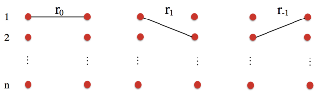
Figure 1: The three building blocks for all connection rules in $\mathsf{G}_{1,n}$. The dots represent excitations. The connectivity of the particular entanglement measures considered dictates that these can only be connected horizontally or diagonally to another dot in the previous or the next row. In a generic graph (for $k=1$), the number of dots in each column is $n$ and each dot on the left must be connected to a single dot on the right. Since only three types of link exist, this restricts the number of contributing graphs. The rules are analogous for $\mathsf{G}_{k,n}$, but in this case we have $k$ copies of this structure which we may represent by having dots of different colours. Then each dot on the left is connected to a dot on the right corresponding to the same copy number but possibly different $k$ (colour), see e.g. Fig. 4.

That is, the graph partition function is

$$\sum_{g}\prod_{m,m^{\prime}}(R_{m,m^{\prime}})^{N_{m,m^{\prime}}(g)}\,,$$ (1)

where the power $N_{m,m^{\prime}}(g)$ is the number of edges connecting copies $m$ to $m^{\prime}$ in the graph $g$. In the present paper, for clarity we concentrate on entanglement measures, so that only cyclic permutations are involved, with $m=m^{\prime}+\ell$ and $\ell\in\{1,0,-1\}$; however the above general statement will be clear from the proofs.

The paper is organised as follows. In section 2 we state and prove the connection between replica negativity and Rényi entanglement entropy of quasiparticle qubit states and graph partition functions. In section 3 we show the general result in a free bosonic quantum field theory of arbitrary dimension. We conclude, and briefly discuss some generalisations, in section 4. In appendix A we analyse some examples of the replica logarithmic negativity and the corresponding graph representation. In appendix B we reproduce the analytic result of the single particle replica negativity presented in [32] through a recursion relation of the graph partition function.

2 Graph partition functions for qubit entanglement

2.1 Definitions and main statement

2.1.1 Graphs

Consider the family of graphs described above (1) in the introduction. As mentioned, we specialise it to the cases which are of immediate use to the evaluation of the replica logarithmic negativity and the Rényi entanglement entropy, giving a precise definition for these cases. Throughout, for every $m\in{\mathbb{N}}$ we denote $I_{m}=\{1,\ldots,m\}$.

Let $k\in{\mathbb{N}}$ and $n\in{\mathbb{N}}$. With respect to the description above (1), $k$ is the number of particles, assuming they all have equal momenta, and $n$ is the number of copies. Consider the set ${\mathsf{G}}_{k,n}$ of all graphs as follows. They are formed by the $2kn$ vertices $\mathsf{V}=\{V_{j,m}^{\epsilon}:j\in I_{k},\;m\in I_{n},\;\epsilon\in\{{\rm l},{\rm r}\}\}$ – two sets, “left” and “right”, of $kn$ vertices – and $kn$ edges. The edges join left to right vertices, and are within the set $\mathsf{E}={\mathsf{E}}_{1}\cup{\mathsf{E}}_{0}\cup{\mathsf{E}}_{-1}$ formed by the union of ${\mathsf{E}}_{\ell}=\{(V_{j,m}^{\rm l},V_{j^{\prime},m+\ell}^{\rm r}):j,j^{\prime}\in I_{k},\;m\in I_{n}\}$ (under the identification $V_{j,n+1}^{{\rm l},{\rm r}}=V_{j,1}^{{\rm l},{\rm r}}$, $V_{j,0}^{{\rm l},{\rm r}}=V_{j,n}^{{\rm l},{\rm r}}$), with the rule that each vertex must be attached to one and only one edge. Note that if $n=2$, then $\mathsf{E}_{1}=\mathsf{E}_{-1}$, and thus in this case $\mathsf{E}={\mathsf{E}}_{1}\cup{\mathsf{E}}_{0}$. For a graph $g\in{\mathsf{G}}_{k,n}$, denote by $N_{\ell}(g),\,\ell\in\{1,0,-1\}$ the number of edges of the graph that are in ${\mathsf{E}}_{\ell}$. We define the following polynomial in three variables $r_{1},r_{0},r_{-1}$, the partition function of $\mathsf{G}_{k,n}$,

$$p_{k,n}(r_{1},r_{0},r_{-1})=\sum_{g\in{\mathsf{G}}_{k,n}}\cdot\left\{\begin{array}[]{ll}\displaystyle\displaystyle\prod_{\ell\in\{1,0,-1\}}r_{\ell}^{N_{\ell}(g)}&(n>2)\\ \displaystyle r_{0}^{N_{0}(g)}(r_{1}+r_{-1})^{N_{1}(g)}&(n=2).\end{array}\right.$$ (2)

Note that for $n=2$, it is the sum $r_{1}+r_{-1}$ that is raised to the power of the number of edges in $\mathsf{E}_{1}=\mathsf{E}_{-1}$.

Below we make the precise connection with entanglement measures and permutation twists. Let us mention already that (2) agrees with (1), if the permutation-twist configuration is such that on a region of volume ratio $r_{1}$, every copy $m$ permutes to $m+1\;{\rm mod}\;n$, on a distinct region of volume ratio $r_{0}$, every copy $m$ permutes to $m$ (identity element), and on a still distinct region of volume ratio $r_{-1}$, every copy $m$ permutes to $m-1\;{\rm mod}\;n$. Making the connection with (1), with $n>2$ we have $R_{m,m+\ell}=r_{\ell}$ with $n=2$ we have $R_{1,1}=r_{0}$, $R_{1,2}=R_{2,1}=r_{1}+r_{-1}$, and in all cases $N_{\ell}(g)=\sum_{m}N_{m,m+\ell}(g)$.

We will also consider the subset $\mathsf{G}_{k,n}^{\prime}\subset\mathsf{G}_{k,n}$, composed of all graphs where all edges lie within the set ${\mathsf{E}}_{1}\cup{\mathsf{E}}_{0}$, with labels $\ell=0,1$. This is a strict subset only if $n>2$. Its partition function is the following polynomial in two variables $r_{1},r_{0}$:

$$p_{k,n}(r_{1},r_{0},0)=\sum_{g\in{\mathsf{G}}_{k,n}^{\prime}}\prod_{\ell\in\{1,0\}}r_{\ell}^{N_{\ell}(g)}\,.$$ (3)

2.1.2 Replica negativity and entanglement entropy

We now define more precisely the entanglement measures we consider.

Consider the Hilbert space ${\cal H}=L^{2}({\mathbb{N}}_{0}^{3})$ (where ${\mathbb{N}}_{0}=\{0,1,2,\ldots\}$). Let us consider the orthonormal basis $\{|\underline{k}\rangle:\underline{k}=(k_{1},k_{0},k_{-1})\in{\mathbb{N}}_{0}^{3}\}$. This orthonormal basis naturally extracts the structure ${\cal H}={\cal H}_{1}\otimes{\cal H}_{0}\otimes{\cal H}_{-1}$, with ${\cal H}_{\ell}\simeq L^{2}({\mathbb{N}}_{0})$, $\ell\in\{1,0,-1\}$ all isomorphic to each other (and to ${\cal H}$), whose orthonormal bases are naturally chosen as $\{|k_{\ell}\rangle:k_{\ell}\in{\mathbb{N}}_{0}\}$. On the subspace ${\cal H}_{1,-1}={\cal H}_{1}\otimes{\cal H}_{-1}$, we define as usual the partial transpose of an operator $A\in{\rm End}({\cal H}_{1}\otimes{\cal H}_{-1})$ by $\langle k_{1},k_{-1}|A^{{\rm T}_{-1}}|k_{1}^{\prime},k_{-1}^{\prime}\rangle=\langle k_{1},k_{-1}^{\prime}|A|k_{1}^{\prime},k_{-1}\rangle$. On ${\cal H}$, we also define, as usual, the partial trace ${\rm Tr}_{{\cal H}_{0}}:{\cal H}\to{\cal H}_{1,-1}$ of a trace-class operator $B\in{\rm End}({\cal H})$ by $\langle k_{1},k_{-1}|{\rm Tr}_{{\cal H}_{0}}(B)|k_{1}^{\prime},k_{-1}^{\prime}\rangle=\sum_{k_{0}=0}^{\infty}\langle k_{1},k_{0},k_{-1}|B|k_{1}^{\prime},k_{0},k_{-1}^{\prime}\rangle$.

Using these, the “$n$-replica logarithmic negativity” $\mathcal{E}_{n}^{|\psi\rangle}$ of tensor factors ${\cal H}_{1}$ and ${\cal H}_{-1}$ in the state $|\psi\rangle\in{\cal H}$ (with $\langle\psi|\psi\rangle=1$) is defined as follows:

$$\exp\big{[}\mathcal{E}_{n}^{|\psi\rangle}\big{]}={\rm Tr}_{{\cal H}_{1,-1}}\Big{[}\Big{(}\big{(}{\rm Tr}_{{\cal H}_{0}}(|\psi\rangle\langle\psi|)\big{)}^{{\rm T}_{-1}}\Big{)}^{n}\Big{]}\,.$$ (4)

The logarithmic negativity provides a partial measure of the entanglement between ${\cal H}_{1}$ and ${\cal H}_{-1}$ [2, 3, 4, 5, 6, 7] and its replica version was first proposed in [21, 22]. The logarithmic negativity can be obtained as the unique analytic continuation of $\mathcal{E}_{2m}^{|\psi\rangle}$ from integer values of $m$ to the value $1/2$, under appropriate specifications on its analytic structure as a function of $m$.

The Rényi entanglement entropy can be defined as a special case of the $n$-replica negativity. The Rényi entanglement entropy between tensor factors ${\cal H}_{1}$ and ${\cal H}_{0}$ in a vector $|\psi\rangle^{\prime}\in{\cal H}_{1}\otimes{\cal H}_{0}$ is simply obtained using the replica negativity of the vector $|\psi\rangle^{\prime}\otimes|0\rangle$ (or any such factorised vector in ${\cal H}$) as follows:

$$S_{n}^{|\psi\rangle^{\prime}}=\frac{\mathcal{E}^{|\psi\rangle^{\prime}\otimes|0\rangle}_{n}}{1-n}\,.$$ (5)

In this factorised case, the trace on tensor factor ${\cal H}_{-1}$ is trivial, and we obtain

$$\exp\big{[}(1-n)S_{n}^{|\psi\rangle^{\prime}}\big{]}={\rm Tr}_{{\cal H}_{1}}\Big{[}\big{(}{\rm Tr}_{{\cal H}_{0}}(|\psi\rangle^{\prime}\ {}^{\prime}\langle\psi|)\big{)}^{n}\Big{]}\,.$$ (6)

2.1.3 Qubit states

We next specify the specific states in ${\cal H}$ whose entanglement measures give graph partition functions.

For $k\in{\mathbb{N}}$ and $r_{1},r_{0},r_{-1}\in[0,1]$ with $r_{1}+r_{0}+r_{-1}=1$, we define the vector

$$|\Psi_{k}(r_{1},r_{0},r_{-1})\rangle=\sum_{\underline{k}=(k_{1},k_{0},k_{-1})\in{\mathbb{N}}_{0}^{3}\atop k_{1}+k_{0}+k_{-1}=k}\sqrt{\frac{k!r_{1}^{k_{1}}r_{0}^{k_{0}}r_{-1}^{k_{-1}}}{k_{1}!k_{0}!k_{-1}!}}|\underline{k}\rangle\in{\cal H}\,.$$ (7)

Note that this vector is normalised:

$$\langle\Psi_{k}(r_{1},r_{0},r_{-1})|\Psi_{k}(r_{1},r_{0},r_{-1})\rangle=\sum_{(k_{1},k_{0},k_{-1})\in{\mathbb{N}}_{0}^{3}\atop k_{1}+k_{0}+k_{-1}=k}\frac{k!r_{1}^{k_{1}}r_{0}^{k_{0}}r_{-1}^{k_{-1}}}{k_{1}!k_{0}!k_{-1}!}=(r_{1}+r_{0}+r_{-1})^{k}=1\,.$$ (8)

This vector represents the “qubit state” for a flat distribution of $k$ indistinguishable particles amongst three complementary regions labelled by $\ell\in\{1,0,-1\}$, which have lengths $r_{\ell}$ adding to 1. The vector $|\underline{k}\rangle$ is associated with the presence of $k_{\ell}$ particles in region $\ell$, and the square of the coefficient, the number $\frac{k!r_{1}^{k_{1}}r_{0}^{k_{0}}r_{-1}^{k_{-1}}}{k_{1}!k_{0}!k_{-1}!}$, with $k_{1}+k_{0}+k_{-1}=k$, is the associated probability that this configuration occurs if we were to place randomly and independently, with uniform distribution, $k$ particles on the interval $[0,1]$ covered by three non-intersecting subintervals of lengths $r_{1},r_{0},r_{-1}$.

In the case where $r_{-1}=0$, then the distribution of the particles is over two non-intersecting regions labelled $\ell\in\{1,0\}$. The resulting vector is of the form

$$|\Psi_{k}(r_{1},r_{0},0)\rangle=|\Psi_{k}(r_{1},r_{0})\rangle^{\prime}\otimes|0\rangle\,.$$ (9)

2.1.4 Theorems

In [32] the following formulae for the $n$-replica logarithmic negativity and the Rényi entropy of the state $|\Psi_{k}(r_{1},r_{0},r_{-1})\rangle$ were proven, starting with the state (7):

Theorem 2.1.

Let $k\in{\mathbb{N}}$, $n\in{\mathbb{N}}$ and $r_{1},r_{0},r_{-1}\in[0,1]$ with $r_{1}+r_{0}+r_{-1}=1$. Then

$$\exp\big{[}\mathcal{E}_{n}^{|\Psi_{k}(r_{1},r_{0},r_{-1})\rangle}\big{]}=\sum_{p=-k}^{k}\sum_{\sigma=\max(0,-np)}^{[\frac{n}{2}(k-p)]}{\mathcal{A}}_{p,\sigma}r_{1}^{np+\sigma}r_{0}^{n(k-p)-2\sigma}r_{-1}^{\sigma}\,.$$ (10)

The coefficients ${\mathcal{A}}_{p,\sigma}$ are

$${\mathcal{A}}_{p,\sigma}=\sum_{\{k_{1},\ldots,k_{n}\}\in P_{n}(\sigma)}\prod_{j=1}^{n}\frac{k!}{(p+k_{j})!(k-p-k_{j+1\;{\rm mod}\;n}-k_{j})!k_{j+1\;{\rm mod}\;n}!}\,,$$ (11)

where $P_{n}(\sigma)$ represents the set of integer partitions of $\sigma$ into $n$ non-negative parts, and by convention the product is set to zero whenever any argument of the factorials is negative. Further,

$$\exp\big{[}(1-n)S_{n}^{|\Psi_{k}(r_{1},r_{0})\rangle^{\prime}}\big{]}=\sum_{j=0}^{k}\left(\frac{k!}{j!(k-j)!}r_{1}^{j}r_{0}^{k-j}\right)^{n}\,.$$ (12)

Note that if $n$ is even, $n=2m$ with $m\in{\mathbb{N}}$, then (10) can be written in a more symmetric fashion,

$$\exp\big{[}\mathcal{E}_{2m}^{|\Psi_{k}(r_{1},r_{0},r_{-1})\rangle}\big{]}=\sum_{p=-k}^{k}\sum_{\sigma=|mp|}^{mk}A_{p,\sigma-mp}r_{1}^{\sigma+mp}r_{0}^{2(mk-\sigma)}r_{-1}^{\sigma-mp}\,.$$ (13)

Note also that the case $r_{-1}=0$ of (10) immediately gives (12).

The main goal of this section is to prove the following theorem: The $n$-replica negativity of the state $|\Psi_{k}(r_{1},r_{0},r_{-1})\rangle$ is proportional to the polynomial (2) up to a simple numerical factor; entanglement is thus related to the combinatoric problem of counting the graphs ${\mathsf{G}}_{k,n}$, and this counting problem leads to the explicit formula (10). The precise mathematical statement is:

Theorem 2.2.

Let $k\in{\mathbb{N}}$, $n\in{\mathbb{N}}$ and $r_{1},r_{0},r_{-1}\in[0,1]$ with $r_{1}+r_{0}+r_{-1}=1$. Then

$$\exp\big{[}\mathcal{E}_{n}^{|\Psi_{k}(r_{1},r_{0},r_{-1})\rangle}\big{]}=\frac{p_{k,n}(r_{1},r_{0},r_{-1})}{(k!)^{n}}\,,$$ (14)

and

$$\exp\big{[}(1-n)S_{n}^{|\Psi_{k}(r_{1},r_{0})\rangle^{\prime}}\big{]}=\frac{p_{k,n}(r_{1},r_{0},0)}{(k!)^{n}}\,.$$ (15)

We note that, again, (15) immediately follows from (14) using (5) and (9), hence below we only prove (14).

2.2 Proof

In this section we will use the notation $k_{\ell}^{(j)}$ where $j$ is the replica number, and for notational convenience, we make the identifications

$$k_{\ell}^{(0)}\equiv k_{\ell}^{(n)},\quad k_{\ell}^{(n+1)}\equiv k_{\ell}^{(1)}\,.$$ (16)

In order to show Theorem 2.2, we show two lemmas.

2.2.1 Permutation twists

First, we re-write the $n$-replica logarithmic negativity in terms of a quantum average, in the state represented by $|\psi\rangle^{\otimes n}$ on the $n$-replica Hilbert space ${\cal H}^{\otimes n}$, of a particular product of permutation operators, permuting the copies and acting on the individual tensor factors ${\cal H}_{\ell}$ – these are the permutation twists. For the entanglement measures, it is sufficient to consider cyclic permutations. We define the operators $\mathbf{P}_{\ell}^{\pm}$ for $\ell\in\{1,0,-1\}$, acting on ${\cal H}^{\otimes n}$ as

$$\mathbf{P}_{\ell}^{\epsilon}\,\bigotimes_{j=1}^{n}|k_{1}^{(j)},k_{0}^{(j)},k_{-1}^{(j)}\rangle=\bigotimes_{j=1}^{n}|k_{1}^{(j-\epsilon\delta_{1,\ell})},k_{0}^{(j-\epsilon\delta_{0,\ell})},k_{-1}^{(j-\epsilon\delta_{-1,\ell})}\rangle,\quad\epsilon\in\{+,-\}\,,$$ (17)

where $\bigotimes_{j=1}^{n}|\underline{k}^{(j)}\rangle=|\underline{k}^{(1)};\ldots;\underline{k}^{(n)}\rangle\in{\cal H}^{\otimes n}$, and with the identifications (16). These operators perform cyclic permutations of the $n$ copies of the individual tensor factors ${\cal H}_{\ell}$; with $\epsilon=+$ ($-$), they shift them rightwards (leftwards). With the notation that the operator ${\cal O}^{(j)}_{\ell}$ acts nontrivially only on the $j^{\rm th}$ tensor factor of ${\cal H}^{\otimes n}$, and on this factor, nontrivially only on the tensor factor ${\cal H}_{\ell}$ of ${\cal H}$, as ${\cal O}\in{\rm End}({\cal H}_{\ell})$, the permutation operators satisfy the exchange relations

$$\mathbf{P}^{\epsilon}_{\ell}{\cal O}^{(j)}_{\ell^{\prime}}=\left\{\begin{array}[]{ll}\displaystyle{\cal O}^{(j+\epsilon)}_{\ell^{\prime}}\mathbf{P}^{\epsilon}_{\ell}&(\ell=\ell^{\prime})\\ {\cal O}^{(j)}_{\ell^{\prime}}\mathbf{P}^{\epsilon}_{\ell}&(\ell\neq\ell^{\prime})\end{array}\right.\,.$$ (18)

The following holds:

Lemma 2.3.

Let $|\psi\rangle\in{\cal H}$ with $\langle\psi|\psi\rangle=1$. Then

$$\exp\big{[}\mathcal{E}_{n}^{|\psi\rangle}\big{]}={}^{\otimes n}\langle\psi|\mathbf{P}_{1}^{+}\mathbf{P}_{-1}^{-}|\psi\rangle^{\otimes n}\,.$$ (19)

Let $|\psi\rangle^{\prime}\in{\cal H}_{1}\otimes{\cal H}_{0}$. Then

$$\exp\big{[}(1-n)S_{n}^{|\psi\rangle^{\prime}}\big{]}={}^{\otimes n}\,{}^{\prime}\langle\psi|\mathbf{P}_{1}^{+}|\psi\rangle^{\prime}{}^{\otimes n}\,,$$ (20)

where by a slight abuse of notation, $\mathbf{P}_{1}^{+}$ is the natural restriction to ${\rm End}({\cal H}_{1}\otimes{\cal H}_{0})$.

Proof.

The proof is obtained by a direct evaluation of both sides. From [32, Eq 3.20], writing $|\psi\rangle=\sum_{\underline{k}\in{\mathbb{N}}_{0}^{3}}c_{\underline{k}}|\underline{k}\rangle$, we have

$$\exp\big{[}\mathcal{E}_{n}^{|\psi\rangle}\big{]}=\sum_{\{k_{\ell}^{(j)}\in{\mathbb{N}}_{0}:\atop\ell\in\{1,0,-1\},j\in I_{n}\}}\prod_{j=1}^{n}c_{k_{1}^{(j+1)},k_{0}^{(j)},k_{-1}^{(j)}}c_{k_{1}^{(j)},k_{0}^{(j)},k_{-1}^{(j+1)}}^{*}\,,$$ (21)

with the convention (16). This gives the left-hand side of (19). On the other hand, we have

$$\mathbf{P}_{1}^{+}\mathbf{P}_{-1}^{-}|\psi\rangle^{\otimes n}=\sum_{\{k_{\ell}^{(j)}\in{\mathbb{N}}_{0}:\atop\ell\in\{1,0,-1\},j\in I_{n}\}}\prod_{j=1}^{n}c_{k_{1}^{(j)},k_{0}^{(j)},k_{-1}^{(j)}}\,\bigotimes_{j=1}^{n}|k_{1}^{(j-1)},k_{0}^{(j)},k_{-1}^{(j+1)}\rangle\,,$$ (22)

which gives rise to

$${}^{\otimes n}\langle\psi|\mathbf{P}_{1}^{+}\mathbf{P}_{-1}^{-}|\psi\rangle^{\otimes n}=\sum_{\{k_{\ell}^{(j)}\in{\mathbb{N}}_{0}:\atop\ell\in\{1,0,-1\},j\in I_{n}\}}\prod_{j=1}^{n}c_{k_{1}^{(j+1)},k_{0}^{(j)},k_{-1}^{(j)}}c_{k_{1}^{(j)},k_{0}^{(j)},k_{-1}^{(j+1)}}^{*}\,,$$ (23)

showing the first part of the lemma. The second part is obtained immediately by using (5).  

Lemma 2.3 makes it clear that, despite the partial transpose used in the definition of the $n$-replica negativity, the result is invariant under unitary transformations of the individual tensor factors of ${\cal H}$ (this is a well-known fact):

Corollary 2.4.

The $n$-replica negativity is invariant under unitary transformations of its factors, $\mathcal{E}_{n}^{|\psi\rangle}=\mathcal{E}_{n}^{U_{1}U_{0}U_{-1}|\psi\rangle}$ for any unitary $U_{\ell}$ acting nontrivially on ${\cal H}_{\ell}$.

2.2.2 Fock space representation

Second, we establish using (19), for rational values of $r_{\ell}$, a representation of the replica logarithmic negativity of the state $|\psi\rangle=|\Psi_{k}(r_{1},r_{0},r_{-1})\rangle$, as that of a new state in a Fock space representing particles on a chain. The Fock-space state is the $k$th power of a uniform sum, over all positions of the system, of position-labelled particle creation operators, representing the idea that particles are uniformly distributed in space. This makes the interpretation of the quasiparticle qubit state (7) clearer, and will directly lead, by the exchange relation (18) and Wick’s theorem, to the graph partition functions (2).

Let $L\in{\mathbb{N}}$, set $X_{-2}=0$ and $X_{1}=L$, and let $X_{-1},X_{0}\in\{1,\ldots,L\}$ such that $X_{\ell-1}<X_{\ell}$ for $\ell=-1,0,1$. Consider the non-intersecting subsets $\mathfrak{R}_{\ell}=\{X_{\ell-1}+1,\ldots,X_{\ell}\}$ for $\ell=-1,0,1$, which have cardinalities $L_{\ell}=|\mathfrak{R}_{\ell}|=X_{\ell}-X_{\ell-1}$ summing to $L_{1}+L_{0}+L_{-1}=L$. Set

$$r_{\ell}=\frac{L_{\ell}}{L},\quad\ell=-1,0,1.$$ (24)

Construct the Fock space ${\cal F}$ with the canonical commutation relations for the operators $a_{x},\,a_{y}\in{\rm End}({\cal F}),\;x,y\in\{1,\ldots,L\}$,

$$[a_{x},a_{y}^{\dagger}]=\delta_{x,y},\quad[a_{x},a_{y}]=[a_{x}^{\dagger},a_{y}^{\dagger}]=0,\quad x,y\in\{1,\ldots,L\}\,,$$ (25)

and with the vacuum $|0\rangle\rangle$ satisfying $a_{x}|0\rangle\rangle=0\;\forall x$. This factorises as ${\cal F}={\cal F}_{1}\otimes{\cal F}_{0}\otimes{\cal F}_{-1}$ into Fock spaces ${\cal F}_{\ell}$ for the generators $\{a_{x},a_{x}^{\dagger}:x\in\mathfrak{R}_{\ell}\}$. As any two countable-dimensional Hilbert spaces are isomorphic, we have isomorphisms ${\cal F}_{\ell}\simeq{\cal H}_{\ell}$ for $\ell=-1,0,1$, and therefore ${\cal F}\simeq{\cal H}$. Let us denote one such isomorphism by $\phi_{\cal F}:{\cal F}\to{\cal H}$, with $\phi_{\cal F}({\cal F}_{\ell})={\cal H}_{\ell}$. We define the permutation twists

$$\mathbf{P}_{\ell}^{\epsilon,{\cal F}}:=\phi_{\cal F}^{-1}\circ\mathbf{P}_{\ell}^{\epsilon}\circ\phi_{\cal F}$$ (26)

on ${\cal F}^{\otimes n}$. This acts, in the natural way, by permutation of the copies on the individual tensor factors ${\cal F}_{\ell}$, and is independent of the choice of $\phi_{\cal F}$. Then, following Lemma 2.3, for any $|\psi\rangle\rangle\in{\cal F}$, we define the $n$-replica logarithmic negativity on ${\cal F}$ by

$$\exp\big{[}\mathcal{E}_{n}^{|\psi\rangle\rangle}\big{]}={}^{\otimes n}\langle\langle\psi|\mathbf{P}_{1}^{+,{\cal F}}\mathbf{P}_{-1}^{-,{\cal F}}|\psi\rangle\rangle^{\otimes n}\,.$$ (27)

Let

$$|\Psi_{k}(r_{1},r_{0},r_{-1})\rangle\rangle=\frac{1}{\sqrt{k!L^{k}}}\Bigg{(}\sum_{x\in\{1,\ldots,L\}}a^{\dagger}_{x}\Bigg{)}^{k}|0\rangle\rangle\in{\cal F}\,.$$ (28)

Writing $\sum_{x\in\{1,\ldots,L\}}=\sum_{x\in\mathfrak{R}_{1}}+\sum_{x\in\mathfrak{R}_{2}}+\sum_{x\in\mathfrak{R}_{3}}$, one can regroup the terms in the following way:

$$|\Psi_{k}(r_{1},r_{0},r_{-1})\rangle\rangle = \frac{1}{\sqrt{k!L^{k}}}\sum_{k_{1},k_{0},k_{-1}\in\{0,\ldots,k\}\atop k_{1}+k_{0}+k_{-1}=k}\frac{k!}{k_{1}!k_{0}!k_{-1}!}\prod_{\ell\in\{1,0,-1\}}\Bigg{(}\sum_{x\in\mathfrak{R}_{\ell}}a_{x}^{\dagger}\Bigg{)}^{k_{\ell}}|0\rangle\rangle$$ (29)

$$= \sum_{k_{1},k_{0},k_{-1}\in\{0,\ldots,k\}\atop k_{1}+k_{0}+k_{-1}=k}\sqrt{\frac{k!r_{1}!r_{2}!r_{3}!}{k_{1}!k_{0}!k_{-1}!}}\prod_{\ell\in\{1,0,-1\}}\frac{1}{\sqrt{k_{\ell}!L_{\ell}^{k_{\ell}}}}\Bigg{(}\sum_{x\in\mathfrak{R}_{\ell}}a_{x}^{\dagger}\Bigg{)}^{k_{\ell}}|0\rangle\rangle\,.$$

We see that this has the structure of the vector $|\Psi_{k}(r_{1},r_{0},r_{-1})\rangle$ defined in (7). This allows us to show the following lemma, which makes the correspondence explicit. Via this correspondence, the nontrivial combinatoric factors in (29) are seen explicitly to occur, using the expression (28), from a uniform distribution of particles in space. This is what will lead, in paragraph 2.2.3, to the proof of the relation with graph partition functions.

Lemma 2.5.

$$\mathcal{E}_{n}^{|\Psi_{k}(r_{1},r_{0},r_{-1})\rangle}=\mathcal{E}_{n}^{|\Psi_{k}(r_{1},r_{0},r_{-1})\rangle\rangle}.$$ (30)

Proof.

In ${\cal F}_{\ell}$, construct the vectors

$$|k_{\ell}\rangle\rangle_{\ell}=\frac{1}{\sqrt{k_{\ell}!L_{\ell}^{k_{\ell}}}}\Bigg{(}\sum_{x\in\mathfrak{R}_{\ell}}a_{x}^{\dagger}\Bigg{)}^{k_{\ell}}|0\rangle\rangle\\ =\sum_{x_{1},\ldots,x_{k_{\ell}}\in\mathfrak{R}_{\ell}}\frac{\Big{(}\prod_{j\in I_{k_{\ell}}}a^{\dagger}_{x_{j}}\Big{)}|0\rangle\rangle}{\sqrt{k_{\ell}!L_{\ell}^{k_{\ell}}}}\in{\cal F}_{\ell}\,.$$

These are orthonormal, ${}_{\ell}\langle\langle k_{\ell}|k_{\ell}^{\prime}\rangle\rangle_{\ell}=\delta_{k_{\ell},k_{\ell}^{\prime}}$. Construct the following vectors in ${\cal F}$:

$$|k_{1},k_{0},k_{-1}\rangle\rangle=|k_{1}\rangle\rangle_{1}\otimes|k_{0}\rangle\rangle_{0}\otimes|k_{-1}\rangle\rangle_{{-1}}\in{\cal F}\,,$$ (31)

which are also orthonormal $\langle\langle k_{1},k_{0},k_{-1}|k_{1}^{\prime},k_{0}^{\prime},k_{-1}^{\prime}\rangle\rangle=\delta_{k_{1},k_{1}^{\prime}}\delta_{k_{0},k_{0}^{\prime}}\delta_{k_{-1},k_{-1}^{\prime}}$. Finally, consider the subspace

$${\cal V}={\rm span}\big{(}|k_{1},k_{0},k_{-1}\rangle\rangle:k_{1},k_{0},k_{-1}\in{\mathbb{N}}_{0}\big{)}\subset{\cal F}\,.$$ (32)

Clearly, there is an isomorphism from ${\cal V}$ onto ${\cal H}$, which can be explicitly written as

$$\begin{array}[]{rcl}\displaystyle\phi_{\cal V}:\quad\qquad\qquad{\cal V}&\to&{\cal H}\\ |k_{1},k_{0},k_{-1}\rangle\rangle&\mapsto&|k_{1},k_{0},k_{-1}\rangle\,.\end{array}$$ (33)

We define $\mathbf{P}_{\ell}^{\epsilon,{\cal V}}$, the permutation twists on ${\cal V}$, in a similar way to (26), using, say, the isomorphism $\phi_{\cal V}$. Clearly, from this definition, $\mathbf{P}_{\ell}^{\epsilon,{\cal V}}|\psi\rangle\rangle^{\otimes n}=\mathbf{P}_{\ell}^{\epsilon,{\cal F}}|\psi\rangle\rangle^{\otimes n}$ for all $|\psi\rangle\rangle\in{\cal V}$. Therefore,

$$\exp\big{[}{\cal E}_{n}^{|\psi\rangle}\big{]} = {}^{\otimes n}\langle\psi|\mathbf{P}_{1}^{+}\mathbf{P}_{-1}^{-}|\psi\rangle^{\otimes n}={}^{\otimes n}\langle\psi|\phi_{\cal V}\mathbf{P}_{1}^{+,{\cal V}}\mathbf{P}_{-1}^{-,{\cal V}}\phi_{\cal V}^{-1}|\psi\rangle^{\otimes n}={}^{\otimes n}\langle\psi|\phi_{\cal V}\mathbf{P}_{1}^{+,{\cal F}}\mathbf{P}_{-1}^{-,{\cal F}}\phi_{\cal V}^{-1}|\psi\rangle^{\otimes n}$$ (34)

$$= \exp\big{[}{\cal E}_{n}^{|\psi\rangle\rangle}\big{]},\qquad|\psi\rangle\rangle=\phi_{\cal V}^{-1}|\psi\rangle\in{\cal V}\subset{\cal F}.$$

Finally, as is clear from (29),

$$\phi_{\cal V}^{-1}|\Psi_{k}(r_{1},r_{0},r_{-1})\rangle=|\Psi_{k}(r_{1},r_{0},r_{-1})\rangle\rangle.$$ (35)

This shows the lemma.  

2.2.3 Proof of theorem 2.2

We use Lemma 2.5 along with (28) and write

$$\exp\big{[}\mathcal{E}_{n}^{|\Psi_{k}(r_{1},r_{0},r_{-1})\rangle}\big{]}={}^{\otimes n}\langle\langle\Psi_{k}(r_{1},r_{0},r_{-1}|\mathbf{P}_{1}^{+,{\cal F}}\mathbf{P}_{-1}^{-,{\cal F}}|\Psi_{k}(r_{1},r_{0},r_{-1}\rangle\rangle^{\otimes n}\,.$$ (36)

The right-hand side is, explicitly,

$$\frac{1}{(k!)^{n}L^{kn}}\Big{(}\sum_{y_{1},\ldots,y_{k}\in I_{L}}\langle\langle 0|\prod_{j\in I_{k}}a_{y_{j}}\Big{)}^{\otimes n}\;\mathbf{P}_{1}^{+,{\cal F}}\mathbf{P}_{-1}^{-,{\cal F}}\;\Big{(}\sum_{x_{1},\ldots,x_{k}\in I_{L}}\prod_{i\in I_{k}}a_{x_{i}}^{\dagger}|0\rangle\rangle\Big{)}^{\otimes n}\,.$$ (37)

Let us denote by $a_{y}^{p}$ and $\big{[}a_{x}^{m}\big{]}^{\dagger}$ the annihilation and creation operators on copy $p,m\in\{1,\ldots,n\}$. Using the exchange relation (18) and the invariance of the state $|0\rangle\rangle^{\otimes n}$ under permutations, we pass the creation operators to the left of the permutation operators and obtain

$$\frac{1}{(k!)^{n}L^{kn}}\sum_{\{y_{j,p}\in I_{L}\}}\sum_{\{x_{i,m}\in I_{L}\}}\langle\langle 0|\prod_{j\in I_{k},\,p\in I_{n}}a_{y_{j,p}}^{p}\prod_{i\in I_{k},\,m\in I_{n}}\Big{[}a_{x_{i,m}}^{m+\chi(x_{i,m}\in\mathfrak{R}_{1})-\chi(x_{i,m}\in\mathfrak{R}_{-1})}\Big{]}^{\dagger}|0\rangle\rangle\,,$$ (38)

where $\chi({\rm c})$ is the indicator function for condition ${\rm c}$, that is 1 if $\rm c$ is true and 0 otherwise. We evaluate this expression by Wick’s theorem. Accordingly, the quantity

$$\sum_{\{y_{j,p}\in I_{L}\}}\sum_{\{x_{i,m}\in I_{L}\}}\langle\langle 0|\prod_{j\in I_{k},\,p\in I_{n}}a_{y_{j,p}}^{p}\prod_{i\in I_{k},\,m\in I_{n}}\Big{[}a_{x_{i,m}}^{m+\chi(x_{i,m}\in\mathfrak{R}_{1})-\chi(x_{i,m}\in\mathfrak{R}_{-1})}\Big{]}^{\dagger}|0\rangle\rangle\,,$$ (39)

is a sum of Wick terms, each term being a product of Wick contractions between creation and annihilation operators, which simply evaluates to 1. We organise this sum as follows. Recall subsection 2.1.1 where we introduced the graphs in $\mathsf{G}_{k,n}$. We identify each pair $j,p$ of labels in the product $\prod_{j\in I_{k},\,p\in I_{n}}a_{y_{j,p}}^{p}$ with the vertex $V_{j,p}^{{\rm r}}$ in $\mathsf{V}$; and likewise we identify each pair $i,m$ of labels in the product $\prod_{i\in I_{k},\,m\in I_{n}}\Big{[}a_{x_{i,m}}^{m+\chi(x_{i,m}\in\mathfrak{R}_{1})-\chi(x_{i,m}\in\mathfrak{R}_{-1})}\Big{]}^{\dagger}$ with the vertex $V_{j,p}^{{\rm l}}$ in $\mathsf{V}$. We also identify each Wick contraction in a Wick term with an edge between these vertices. Thus each Wick term is unambiguously a graph with edges connecting vertices in $\mathsf{V}$. There is a contraction between $a_{y_{j,p}}^{p}$ and $\Big{[}a_{x_{i,m}}^{m+\chi(x_{i,m}\in\mathfrak{R}_{-1})-\chi(x_{i,m}\in\mathfrak{R}_{1})}\Big{]}^{\dagger}$ if and only if $y_{j,p}=x_{i,m}$ and $p=m+\chi(x_{i,m}\in\mathfrak{R}_{1})-\chi(x_{i,m}\in\mathfrak{R}_{-1})$. Therefore, either $p=m$, or $p=m+1$, or $p=m-1$. There are no other contractions. Hence, each edge is in $\mathsf{E}_{1}\cup\mathsf{E}_{0}\cup\mathsf{E}_{-1}$ (and $p=m+\ell$ corresponds to an edge in $\mathsf{E}_{\ell}$), as illustrated by Fig. 1. Further, by Wick’s theorem, every vertex is the end-point of one and only one edge. Therefore, each Wick term is identified with a graph in $\mathsf{G}_{n,k}$, and each such term evaluates to 1.

We now need to count how many times $N(g)$ a given graph $g\in\mathsf{G}_{n,k}$ occurs in the sum of Wick terms; then the result is written as

$$\sum_{\{y_{j,p}\in I_{L}\}}\sum_{\{x_{i,m}\in I_{L}\}}\langle\langle 0|\prod_{j\in I_{k},\,p\in I_{n}}a_{y_{j,p}}^{p}\prod_{i\in I_{k},\,m\in I_{n}}\Big{[}a_{x_{i,m}}^{m+\chi(x_{i,m}\in\mathfrak{R}_{-1})-\chi(x_{i,m}\in\mathfrak{R}_{1})}\Big{]}^{\dagger}|0\rangle\rangle=\sum_{g\in\mathsf{G}_{n,k}}N(g)\,.$$

For every edge $(V_{i,m}^{{\rm l}},V_{j,p}^{{\rm r}})$, there is a factor coming from the sum over the possible values of $y_{j,p}$ and $x_{i,m}$ leading to this edge. Because of the condition $y_{j,p}=x_{i,m}$, we only need to consider one sum. Because of the condition $p=m+\chi(x_{i,m}\in\mathfrak{R}_{1})-\chi(x_{i,m}\in\mathfrak{R}_{-1})$, the values of $y_{j,p}$ leading to this edge are all values $y_{j,p}\in\mathfrak{R}_{0}$ if $p=m$, all values $y_{j,p}\in\mathfrak{R}_{1}$ if $p=m+1$, and all values $y_{j,p}\in\mathfrak{R}_{-1}$ if $p=m-1$. Thus, if $n>2$, for each edge in $\mathsf{E}_{\ell}$, there is a factor $|\mathfrak{R}_{\ell}|=L_{\ell}$; and if $n=2$, then for each edge in $\mathsf{E}_{1}=\mathsf{E}_{-1}$, there is a factor $L_{1}+L_{-1}$. Since there are exactly $kn$ edges, we obtain, for $n>2$,

$$\sum_{\{y_{j,p}\in I_{L}\}}\sum_{\{x_{i,m}\in I_{L}\}}\langle\langle 0|\prod_{j\in I_{k},\,p\in I_{n}}a_{y_{j,p}}^{p}\prod_{i\in I_{k},\,m\in I_{n}}\Big{[}a_{x_{i,m}}^{m+\chi(x_{i,m}\in\mathfrak{R}_{-1})-\chi(x_{i,m}\in\mathfrak{R}_{1})}\Big{]}^{\dagger}|0\rangle\rangle=L^{kn}\sum_{g\in\mathsf{G}_{n,k}}r_{\ell}^{N_{\ell}(g)}\,,$$

where we recall $r_{\ell}=L_{\ell}/L$ and $N_{\ell}(g)$ is the number of edges in $g$ that lie in $\mathsf{E}_{\ell}$; and thus

$$\exp\big{[}\mathcal{E}_{n}^{|\Psi_{k}(r_{1},r_{0},r_{-1})\rangle}\big{]}=\frac{1}{(k!)^{n}}\sum_{g\in\mathsf{G}_{k,n}}r_{\ell}^{N_{\ell}(g)}=\frac{p_{k,n}(r_{1},r_{0},r_{-1})}{(k!)^{n}}\,.$$ (40)

For $n=2$, a similar argument leads again to $\frac{p_{k,2}(r_{1},r_{0},r_{-1})}{(k!)^{2}}$.  

3 Entanglement of particle excitations in free bosonic quantum field theory

3.1 Main statement

Consider the massive free boson of mass $m$ on the hypertorus ${\mathfrak{M}}=\times_{j=1}^{d}[0,L_{j}]\subset{\mathbb{R}}^{d}$ of dimension $d\geq 1$ (space-time having dimension $d+1$). For simplicity we assume that there is some UV regularisation, for instance a harmonic lattice. We will not need to specify any particular regularisation, since the derivation holds true as long as the general properties stated below remain valid. This in fact serves to illustrate the generality of the method, beyond the realm of UV-completed field theory.

We denote by $\lambda{\mathfrak{M}}$ the hypertorus scaled by the factor $\lambda>1$. Consider two non-intersecting open subsets ${\mathfrak{R}}_{1},\;{\mathfrak{R}}_{-1}\subset{\mathfrak{M}}$, of any connectivity, and similarly denote by $\lambda{\mathfrak{R}}_{1}$ and $\lambda{\mathfrak{R}}_{1}$ the scaled subsets of $\lambda{\mathfrak{M}}$. For simplicity of the argument, we assume that the regions ${\mathfrak{R}}_{1},\;{\mathfrak{R}}_{-1}$ have piecewise smooth boundaries.

It is a simple matter to construct the vacuum state $|{\rm vac}\rangle$ and multi-particle excited states $|\bm{p}_{1},\ldots\bm{p}_{k}\rangle$ in this theory via the Fock space ${\cal H}$ over the canonical algebra of annihilation and creation operators $A_{\bm{p}}$ and $A^{\dagger}_{\bm{p}}$ at momenta $\bm{p}\in\Lambda_{d}\subset{\mathbb{R}}^{d}$. The momenta are quantised to the square lattice $\Lambda_{d}=\times_{j=1}^{d}(2\pi L_{j}^{-1}{\mathbb{Z}})$, and on $\lambda{\cal M}$ they are quantised to $\lambda^{-1}\Lambda_{d}$. We have

$$[A_{\bm{p}},A^{\dagger}_{\bm{p}^{\prime}}]=\delta_{\bm{p},\bm{p}^{\prime}},\quad A_{\bm{p}}|{\rm vac}\rangle=0,\quad|\bm{p}_{1},\ldots\bm{p}_{k}\rangle=A^{\dagger}_{\bm{p}_{1}}\cdots A^{\dagger}_{\bm{p}_{k}}|{\rm vac}\rangle\,.$$ (41)

These operators can be written in terms of the Klein-Gordon field $\Phi(\bm{x})$ and its canonical conjugate $\Pi(\bm{x})$ as

$$A_{\bm{p}}=\frac{1}{\sqrt{{\rm Vol}(\mathfrak{M})}}\int_{{\mathfrak{M}}}{\rm d}^{d}\bm{x}\,{\rm e}^{-{\rm i}\bm{p}\cdot\bm{x}}{\cal O}_{\bm{p}}(\bm{x})\,,$$ (42)

where

$${\cal O}_{\bm{p}}(\bm{x})=\frac{E_{\bm{p}}\Phi(\bm{x})+{\rm i}\Pi(\bm{x})}{\sqrt{2E_{\bm{p}}}}\,,$$ (43)

with $E_{\bm{p}}$ the energy. In the relativistic boson, it obeys the relativistic dispersion relation $E_{\bm{p}}=\sqrt{m^{2}+\bm{p}^{2}}$, but this is not necessary for the proof; other dispersion relations, such as that from the harmonic lattice, can be used. All states are normalised to 1.

We are interested in the increment of entanglement between two regions due to the presence of a finite number of particles. Thus we would like to evaluate the difference of replica logarithmic negativities, and of Rényi entropies, between a $k$-particle state and the vacuum $|{\rm vac}\rangle$. The clearest way to define the replica entanglement negativity and the Rényi entanglement entropy in QFT is to use their general expressions in terms of permutation twists, shown in Lemma 2.3. We simply identify the tensor factors ${\cal H}_{\ell}$ with the spaces of field configurations on the regions ${\mathfrak{R}}_{\ell}$, $\ell\in\{1,-1\}$; in general we will denote by $\mathbf{P}^{\epsilon}(\mathfrak{R})$ the permutation twists associated to the tensor factors of field configurations supported on $\mathfrak{R}$. As we have assumed that there is some UV regularisation, no divergence occurs in averages of such permutation twists. In 1+1-dimensional quantum field theory, $\mathbf{P}^{\epsilon}(\mathfrak{R})$ is the product of appropriate branch-point twist fields positioned at the boundary points of $\mathfrak{R}$ [13, 14].

Consider a set of momenta $\mathsf{p}=\{\bm{p}_{1},\ldots,\bm{p}_{k}\}$ with $\bm{p}_{j}\in\Lambda_{d}$. We wish to evaluate, in an appropriate limit, the following replica logarithmic negativity and Rényi entropy increments,

$$\exp\big{[}\Delta\mathcal{E}_{n}^{|\mathsf{p}\rangle}({\mathfrak{R}}_{1},{\mathfrak{R}}_{-1};{\mathfrak{M}})\big{]}=\frac{{}^{\otimes n}\langle\mathsf{p}|\mathbf{P}^{+}(\mathfrak{R}_{1})\mathbf{P}^{-}(\mathfrak{R}_{-1})|\mathsf{p}\rangle^{\otimes n}}{{}^{\otimes n}\langle\mathsf{p}|\mathsf{p}\rangle^{\otimes n}\ {}^{\otimes n}\langle{\rm vac}|\mathbf{P}^{+}(\mathfrak{R}_{1})\mathbf{P}^{-}(\mathfrak{R}_{-1})|{\rm vac}\rangle^{\otimes n}}\,,$$ (44)

and

$$\exp\big{[}(1-n)\Delta S_{n}^{|\mathsf{p}\rangle}({\mathfrak{R}}_{1};{\mathfrak{M}})\big{]}=\frac{{}^{\otimes n}\langle\mathsf{p}|\mathbf{P}^{+}(\mathfrak{R}_{1})|\mathsf{p}\rangle^{\otimes n}}{{}^{\otimes n}\langle\mathsf{p}|\mathsf{p}\rangle^{\otimes n}\ {}^{\otimes n}\langle{\rm vac}|\mathbf{P}^{+}(\mathfrak{R}_{1})|{\rm vac}\rangle^{\otimes n}}\,,$$ (45)

respectively.

In order to study these objects, we need some facts about the permutation twists in the $n$-copy massive free boson.

The main properties of the operators $\mathbf{P}^{\epsilon}(\mathfrak{R}_{\ell})$ are the exchange relations (18), which here can be written

$$\mathbf{P}^{\epsilon}(\mathfrak{R}_{\ell}){\cal O}^{(j)}(\bm{x})=\left\{\begin{array}[]{ll}\displaystyle{\cal O}^{(j+\epsilon)}(\bm{x})\mathbf{P}^{\epsilon}(\mathfrak{R}_{\ell})&(\bm{x}\in\mathfrak{R}_{\ell})\\ {\cal O}^{(j)}(\bm{x})\mathbf{P}^{\epsilon}(\mathfrak{R}_{\ell})&(\bm{x}\in\mathfrak{M}\setminus\mathfrak{R}_{\ell})\,.\end{array}\right.$$ (46)

In this notation, ${\cal O}^{(j)}(\bm{x})$ is defined by acting nontrivially only on the $j^{\rm th}$ tensor factor of ${\cal H}^{\otimes n}$, and on this factor, it acts as the local operator ${\cal O}(\bm{x})\in{\rm End}(\cal H)$ positioned at $\bm{x}\in\mathfrak{M}$. The set of fields formed by ${\cal O}^{(j)}(\bm{x})$ with ${\cal O}(\bm{x})\in\{{\bf 1},\,{\cal O}_{\bm{p}}(\bm{x}),{\cal O}_{\bm{p}}(\bm{x})^{\dagger}:{\bm{p}}\in\Lambda_{d},\,\bm{x}\in\mathfrak{M}\}$ and their products spans a dense subset of ${\rm End}({\cal H})^{\otimes n}$.

Because the theory has nonzero mass, all correlation functions of local operators factorise into products of correlation functions exponentially fast with the distance between operators. Something similar is expected (and verified in one dimension) to hold for the permutation operator. Let us express some of these clustering properties more precisely, in a way that is convenient for the proof below.

Consider the normalised correlation function

$${}_{\mathbf{P}}\langle{\cal O}_{\bm{p}_{1}}^{(j_{1})}(\bm{x}_{1})\cdots{\cal O}_{\bm{p}_{k}}^{(j_{k})}(\bm{x}_{k})\rangle_{\mathbf{P}}=\frac{{}^{\otimes n}\langle{\rm vac}|{\cal O}_{\bm{p}_{1}}^{(j_{1})}(\bm{x}_{1})\cdots{\cal O}_{\bm{p}_{k}}^{(j_{k})}(\bm{x}_{k})\mathbf{P}^{+}(\mathfrak{R}_{1})\mathbf{P}^{-}(\mathfrak{R}_{-1})|{\rm vac}\rangle^{\otimes n}}{{}^{\otimes n}\langle{\rm vac}|\mathbf{P}^{+}(\mathfrak{R}_{1})\mathbf{P}^{-}(\mathfrak{R}_{-1})|{\rm vac}\rangle^{\otimes n}\,.}.$$

The insertion of permutation operators is seen as changing the state (the measure) over which we take the average.

The first expected clustering property is that, when the points $\bm{x}_{j}$ are far from the boundaries of the regions $\partial\mathfrak{R}_{1}$ and $\partial\mathfrak{R}_{-1}$, we recover the vacuum state. That is, for every $k\geq 1$ and every set $\{\bm{p}_{1},\ldots,\bm{p}_{k}\}$ of elements of $\Lambda_{d}$, there exists a function $U(\bm{x}_{1},\ldots,\bm{x}_{k})>0$ and a number $V>0$ such that for every set $\{\bm{x}_{1},\ldots,\bm{x}_{k}\}$ of elements of $\mathfrak{M}$, and for every regions $\mathfrak{R}_{1}$ and $\mathfrak{R}_{-1}$ as described above,

$$\Big{|}{}_{\mathbf{P}}\langle{\cal O}_{\bm{p}_{1}}^{(j_{1})}(\bm{x}_{1})\cdots{\cal O}_{\bm{p}_{k}}^{(j_{k})}(\bm{x}_{k})\rangle_{\mathbf{P}}-{}^{\otimes n}\langle{\rm vac}|{\cal O}_{\bm{p}_{1}}^{(j_{1})}(\bm{x}_{1})\cdots{\cal O}_{\bm{p}_{k}}^{(j_{k})}(\bm{x}_{k})|{\rm vac}\rangle^{\otimes n}\Big{|}$$

$$<\ U(\bm{x}_{1},\ldots,\bm{x}_{k})\,\exp\big{[}-V{\rm dist}(\{\bm{x}_{i}:i\in I_{k}\},\partial\mathfrak{R}_{1}\cup\partial\mathfrak{R}_{-1})\big{]}\,.$$ (47)

This clustering at large distance between the points $\bm{x}_{i}$ and the boundary of the regions $\mathfrak{R}_{1}$ and $\mathfrak{R}_{-1}$ indicates that the operator $\mathbf{P}^{+}(\mathfrak{R}_{1})\mathbf{P}^{-}(\mathfrak{R}_{-1})$ is essentially supported on $\partial\mathfrak{R}_{1}\cup\partial\mathfrak{R}_{-1}$. This is expected, as the cyclic permutation of copies is a symmetry of the $n$-copy QFT, and thus $\mathbf{P}^{+}(\mathfrak{R}_{1})\mathbf{P}^{-}(\mathfrak{R}_{-1})$ is a twist operator supported on the boundary of the permutation region.

Second, the function $U(\bm{x}_{1},\ldots,\bm{x}_{k})$ can also be bounded. This is because we expect the new state ${}_{\mathbf{P}}\langle\cdots\rangle_{\mathbf{P}}$, like the vacuum, to still satisfy the clustering property of local fields. The initial observation is that, if the points $\bm{x}_{i}$ are all very far from each other, the normalised correlation function factorises into the averages, in this new state, of each local observable. By the ${\mathbb{Z}}_{2}$ symmetry of the Klein-Gordon theory, acting as ${\cal O}_{\bm{p}}(\bm{x})\mapsto-{\cal O}_{\bm{p}}(\bm{x})$ and preserving the vacuum and the permutation operators, the result vanishes. This vanishing is also exponential. We then conclude that the only way not to have a vanishing result is if for every $i\in I_{k}$ there exists a $j\in I_{k}$ such that ${\rm dist}(\bm{x}_{i},\bm{x}_{j})$ is finite, so that clustering occurs in groups of local fields with nonzero averages. In order to bound the resulting exponential decay due to these various groups, we can simply sum over every minimal distance between a point $\bm{x}_{i}$ and the rest. Hence there exists a $U_{0}>0$ and $W>0$ such that

$$U(\bm{x}_{1},\ldots,\bm{x}_{k})<U_{0}\exp\Big{[}-W\sum_{i\in I_{k}}{\rm dist}\big{(}\bm{x}_{i},\{\bm{x}_{j}:j\in I_{k}\setminus\{i\}\}\big{)}\Big{]}\,,$$ (48)

for all $\{\bm{x}_{i}\in\mathfrak{M}\}$.

Using these properties, we show the following, which gives results for the replica logarithmic negativity increment for the entanglement between the scaled regions $\lambda\mathfrak{R}_{1}$ and $\lambda\mathfrak{R}_{-1}$, and the Rényi entanglement entropy increment for the entanglement between the scaled regions $\lambda\mathfrak{R}_{1}$ and $\lambda\mathfrak{M}\setminus\lambda\mathfrak{R}_{1}$, in the limit where the scaling $\lambda$ tends to infinity.

Theorem 3.1.

Let $\mathsf{p}=\{\bm{p}_{1},\ldots,\bm{p}_{k}\}$ with $\bm{p}_{j}\in{\mathbb{R}}^{d}$, and denote by $[\bm{p}_{j}]_{\lambda}$ the point in $\lambda^{-1}\Lambda_{d}$ that is nearest to $\bm{p}_{j}$, and by $[\mathsf{p}]_{\lambda}=\{[\bm{p}_{1}]_{\lambda},\ldots,\bm{[}\bm{p}_{k}]_{\lambda}\}$. Without loss of generality, assume that $\mathsf{p}$ is formed by groups of identical momenta, $\bm{p}_{1}=\ldots=\bm{p}_{k_{1}}$, $\bm{p}_{k_{1}+1}=\ldots=\bm{p}_{k_{1}+k_{2}}$, $\cdots$ with $\sum_{i}k_{i}=k$, and with momenta belonging to different groups being different. Let $r_{\ell}={\rm Vol}({\mathfrak{R}}_{\ell})/{\rm Vol}({\mathfrak{M}})$ for $\ell\in\{1,-1\}$ and $r_{0}=1-r_{1}-r_{-1}$. Then

$$\lim_{\lambda\to\infty}\Delta\mathcal{E}_{n}^{|[\mathsf{p}]_{\lambda}\rangle}(\lambda{\mathfrak{R}}_{1},\lambda{\mathfrak{R}}_{-1};\lambda{\mathfrak{M}})=\sum_{i}\mathcal{E}_{n}^{|\Psi_{k_{i}}(r_{1},r_{0},r_{-1})\rangle}\,.$$ (49)

Let $r_{1}={\rm Vol}({\mathfrak{R}}_{1})/{\rm Vol}({\mathfrak{M}})$ and $r_{0}=1-r_{1}$. Then

$$\lim_{\lambda\to\infty}\Delta S_{n}^{|[\mathsf{p}]_{\lambda}\rangle}(\lambda{\mathfrak{R}}_{1};\lambda{\mathfrak{M}})=\sum_{i}S_{n}^{|\Psi_{k_{i}}(r_{1},r_{0})\rangle^{\prime}}\,.$$ (50)

Recall the expressions for the qubit entanglement quantities $\mathcal{E}_{n}^{|\Psi_{k_{i}}(r_{1},r_{0},r_{-1})\rangle}$ and $S_{n}^{|\Psi_{k_{i}}(r_{1},r_{0})\rangle^{\prime}}$ in Theorems 2.1 and 2.2.

3.2 Proof

We concentrate on the replica negativity; the entanglement entropy is obtained again as a special case. The idea of the proof is to use the expression (44), where the particle states are explicitly written in terms of local operators as per (42). We then use the exchange relations (46) on the local operators, and evaluate the leading large-$\lambda$ behaviour using the clustering properties. There, the expression is transformed into a vacuum expectation value, with appropriately shifted copy indices, very similar to (39) obtained in the qubit analysis. The creation and annihilation operators are instead local fields, but the evaluation is again by Wick’s theorem. We then analyse the Wick contractions, finding a structure similar to that obtained by evaluating (39). Besides the re-writing into local fields, there is one additional subtlety, as particles carry momenta. We show that particles with different momenta, in the large-$\lambda$ limit, do not Wick contract, and thus the result factorises into groups of equal momenta. In each group, the ensuing graph analysis goes through essentially unchanged.

Using (42),

$${}^{\otimes n}\langle[\mathsf{p}]_{\lambda}|\mathbf{P}^{+}(\lambda\mathfrak{R}_{1})\mathbf{P}^{-}(\lambda\mathfrak{R}_{-1})|[\mathsf{p}]_{\lambda}\rangle^{\otimes n}$$

$$= \frac{1}{\lambda^{dkn}{\rm Vol}(\mathfrak{M})^{kn}}\,\left(\prod_{j=1}^{k}\prod_{i=1}^{n}\int_{\lambda\mathfrak{M}}{\rm d}^{d}\bm{x}_{j}^{(i)}\int_{\lambda\mathfrak{M}}{\rm d}^{d}\bm{y}_{j}^{(i)}\right)\,{\rm e}^{-{\rm i}\sum_{j=1}^{k}\sum_{i=1}^{n}[\bm{p}_{j}]_{\lambda}\cdot(\bm{x}_{j}^{(i)}-\bm{y}_{j}^{(i)})}\,\times$$

$$\times\ {}^{\otimes n}\langle{\rm vac}|\Bigg{(}\prod_{j=1}^{k}\prod_{i=1}^{n}{\cal O}_{[\bm{p}_{j}]_{\lambda}}^{(i)}(\bm{x}_{j}^{(i)})\Bigg{)}\,\Bigg{(}\prod_{j^{\prime}=1}^{k}\prod_{i^{\prime}=1}^{n}\left[{\cal O}_{[\bm{p}_{j^{\prime}}]_{\lambda}}^{(i^{\prime}+\chi(y_{j^{\prime}}^{(i^{\prime})}\in\lambda\mathfrak{R}_{1})-\chi(y_{j^{\prime}}^{(i^{\prime})}\in\lambda\mathfrak{R}_{-1}))}(\bm{y}_{j^{\prime}}^{(i^{\prime})})\right]^{\dagger}\Bigg{)}\,\times$$

$$\quad\qquad\times\ \mathbf{P}^{+}(\lambda\mathfrak{R}_{1})\mathbf{P}^{-}(\lambda\mathfrak{R}_{-1})|{\rm vac}\rangle^{\otimes n}\,.$$

The first step is to show that, in the large $\lambda$ limit, the expectation in the integrand can be factorised into a vacuum expectation value of the local observables, times that of the permutation twists. This is done by using (47), and arguing that the integration over the bulk of the regions, far from the boundaries $\partial\mathfrak{R}_{1,-1}$, is that which dominates. We therefore consider the difference

$$D_{\lambda}(\{\bm{x}^{(i)}_{j},\bm{y}^{(i^{\prime})}_{j^{\prime}}\})=$$

$${}^{\otimes n}\langle{\rm vac}|\Bigg{(}\prod_{j=1}^{k}\prod_{i=1}^{n}{\cal O}_{[\bm{p}_{j}]_{\lambda}}^{(i)}(\bm{x}_{j}^{(i)})\Bigg{)}\,\Bigg{(}\prod_{j^{\prime}=1}^{k}\prod_{i^{\prime}=1}^{n}\left[{\cal O}_{[\bm{p}_{j^{\prime}}]_{\lambda}}^{(i^{\prime}+\chi(y_{j^{\prime}}^{(i^{\prime})}\in\lambda\mathfrak{R}_{1})-\chi(y_{j^{\prime}}^{(i^{\prime})}\in\lambda\mathfrak{R}_{-1}))}(\bm{y}_{j^{\prime}}^{(i^{\prime})})\right]^{\dagger}\Bigg{)}\,\times$$

$$\quad\qquad\times\ \mathbf{P}^{+}(\lambda\mathfrak{R}_{1})\mathbf{P}^{-}(\lambda\mathfrak{R}_{-1})|{\rm vac}\rangle^{\otimes n}\;/\;{}^{\otimes n}\langle{\rm vac}|\mathbf{P}^{+}(\lambda\mathfrak{R}_{1})\mathbf{P}^{-}(\lambda\mathfrak{R}_{-1})|{\rm vac}\rangle^{\otimes n}$$

$$-\ {}^{\otimes n}\langle{\rm vac}|\Bigg{(}\prod_{j=1}^{k}\prod_{i=1}^{n}{\cal O}_{[\bm{p}_{j}]_{\lambda}}^{(i)}(\bm{x}_{j}^{(i)})\Bigg{)}\,\Bigg{(}\prod_{j^{\prime}=1}^{k}\prod_{i^{\prime}=1}^{n}\left[{\cal O}_{[\bm{p}_{j^{\prime}}]_{\lambda}}^{(i^{\prime}+\chi(y_{j^{\prime}}^{(i^{\prime})}\in\lambda\mathfrak{R}_{1})-\chi(y_{j^{\prime}}^{(i^{\prime})}\in\lambda\mathfrak{R}_{-1}))}(\bm{y}_{j^{\prime}}^{(i^{\prime})})\right]^{\dagger}\Bigg{)}|{\rm vac}\rangle^{\otimes n}\,,$$

and, recalling (47), we have

$$\left|\frac{1}{\lambda^{dkn}{\rm Vol}(\mathfrak{M})^{kn}}\,\left(\prod_{j=1}^{k}\prod_{i=1}^{n}\int_{\lambda\mathfrak{M}}{\rm d}^{d}\bm{x}_{j}^{(i)}\int_{\lambda\mathfrak{M}}{\rm d}^{d}\bm{y}_{j}^{(i)}\right)\,{\rm e}^{-{\rm i}\sum_{j=1}^{k}\sum_{i=1}^{n}[\bm{p}_{j}]_{\lambda}\cdot(\bm{x}_{j}^{(i)}-\bm{y}_{j}^{(i)})}D_{\lambda}(\{\bm{x}^{(i)}_{j},\bm{y}^{(i^{\prime})}_{j^{\prime}}\})\right|$$

$$< \frac{1}{\lambda^{dkn}{\rm Vol}(\mathfrak{M})^{kn}}\,\left(\prod_{j=1}^{k}\prod_{i=1}^{n}\int_{\lambda\mathfrak{M}}{\rm d}^{d}\bm{x}_{j}^{(i)}\int_{\lambda\mathfrak{M}}{\rm d}^{d}\bm{y}_{j}^{(i)}\right)\,\left|D_{\lambda}(\{\bm{x}^{(i)}_{j},\bm{y}^{(i^{\prime})}_{j^{\prime}}\})\right|$$

$$< E_{\lambda}\quad=\quad\frac{1}{\lambda^{dkn}{\rm Vol}(\mathfrak{M})^{kn}}\,\prod_{j=1}^{k}\prod_{i=1}^{n}\left(\int_{\lambda\mathfrak{M}}{\rm d}^{d}\bm{x}_{j}^{(i)}\int_{\lambda\mathfrak{M}}{\rm d}^{d}\bm{y}_{j}^{(i)}\right)\,\times$$

$$\qquad\times\ \prod_{j=1}^{k}\prod_{i=1}^{n}\Big{(}U(\{\bm{x}_{j}^{(i)},\bm{y}_{j}^{(i)}\})\,\exp\big{[}-V{\rm dist}(\{\bm{x}_{j}^{(i)},\bm{y}_{j}^{(i)}:j\in I_{k},\,i\in I_{n}\},\partial\mathfrak{R}_{1}\cup\partial\mathfrak{R}_{-1})\big{]}\Big{)}\,,$$

where the function $U$ is bounded as per (48). We now show that

$$\lim_{\lambda\to\infty}E_{\lambda}=0\,.$$ (52)

Thanks to the bound (48), the integrals over the variables $\bm{x}_{j}^{(i)}$’s and $\bm{y}_{j}^{(i)}$’s, lying on the manifold $(\lambda\mathfrak{M})^{\times 2kn}$ of dimension $2dkn$, are supported, with exponential accuracy, over a submanifold which is at most of dimension $dkn$. Indeed, since every variable must lie near to at least one other, one forms pairs or larger groups of nearby variables; forming pairs leads to the largest submanifold, and the dimension of this submanifold is that of the original integration manifold $(\lambda\mathfrak{M})^{\times 2kn}$ divided by 2. Further, thanks to the exponential in (LABEL:corrterm), one further restricts all variables to lie near the boundary of $\mathfrak{R}_{1}$ or $\mathfrak{R}_{-1}$, thus near a submanifold of codimension 1. The remaining integration region is therefore an effectively finite neighborhood (thanks to exponential accuracy) of a submanifold of $(\lambda\mathfrak{M})^{\times 2kn}$ of dimension $dkn-1$. As $\lambda\to\infty$, this scales like $\lambda^{dkn-1}$. Because of the factor $\lambda^{dkn}$ in the denominator in (LABEL:corrterm), the result vanishes as $\lambda\to\infty$.

Therefore, using (47), we find

$$\frac{{}^{\otimes n}\langle[\mathsf{p}]_{\lambda}|\mathbf{P}^{+}(\lambda\mathfrak{R}_{1})\mathbf{P}^{-}(\lambda\mathfrak{R}_{-1})|[\mathsf{p}]_{\lambda}\rangle^{\otimes n}}{{}^{\otimes n}\langle{\rm vac}|\mathbf{P}^{+}(\lambda\mathfrak{R}_{1})\mathbf{P}^{-}(\lambda\mathfrak{R}_{-1})|{\rm vac}\rangle^{\otimes n}}$$ (53)

$$= \frac{1}{\lambda^{dkn}{\rm Vol}(\mathfrak{M})^{kn}}\,\left(\prod_{j=1}^{k}\prod_{i=1}^{n}\int_{\lambda\mathfrak{M}}{\rm d}^{d}\bm{x}_{j}^{(i)}\int_{\lambda\mathfrak{M}}{\rm d}^{d}\bm{y}_{j}^{(i)}\right)\,{\rm e}^{-{\rm i}\sum_{j=1}^{k}\sum_{i=1}^{n}[\bm{p}_{j}]_{\lambda}\cdot(\bm{x}_{j}^{(i)}-\bm{y}_{j}^{(i)})}\,\times$$

$$\times\ {}^{\otimes n}\langle{\rm vac}|\Bigg{(}\prod_{j=1}^{k}\prod_{i=1}^{n}{\cal O}_{[\bm{p}_{j}]_{\lambda}}^{(i)}(\bm{x}_{j}^{(i)})\Bigg{)}\,\Bigg{(}\prod_{j^{\prime}=1}^{k}\prod_{i^{\prime}=1}^{n}\left[{\cal O}_{[\bm{p}_{j^{\prime}}]_{\lambda}}^{(i^{\prime}+\chi(y_{j^{\prime}}^{(i^{\prime})}\in\lambda\mathfrak{R}_{1})-\chi(y_{j^{\prime}}^{(i^{\prime})}\in\lambda\mathfrak{R}_{-1}))}(\bm{y}_{j^{\prime}}^{(i^{\prime})})\right]^{\dagger}\Bigg{)}|{\rm vac}\rangle^{\otimes n}$$

$$+\;O(\lambda^{-1})\,.$$

The correlation function in (53) is evaluted by Wick’s theorem. Every Wick contraction between operators ${\cal O}_{[\bm{p}_{j}]_{\lambda}}^{(i)}(\bm{x}_{j}^{(i)})$ and ${\cal O}_{[\bm{p}_{\tilde{j}}]_{\lambda}}(\bm{x}_{\tilde{j}}^{(\tilde{i})})$ gives exactly, under integrations over $\bm{x}_{j}^{(i)}$ and $\bm{x}_{\tilde{j}}^{(\tilde{i})}$, the overlap $\langle{\rm vac}|A_{p_{j}}A_{p_{\tilde{j}}}|{\rm vac}\rangle$, which vanishes. Hence all operators ${\cal O}_{[\bm{p}_{j}]_{\lambda}}^{(i)}(\bm{x}_{j}^{(i)})$ must be contracted with operators $\left[{\cal O}_{[\bm{p}_{j^{\prime}}]_{\lambda}}^{(i^{\prime}+\chi(y_{j^{\prime}}^{(i^{\prime})}\in\lambda\mathfrak{R}_{1})-\chi(y_{j^{\prime}}^{(i^{\prime})}\in\lambda\mathfrak{R}_{-1}))}(\bm{y}_{j^{\prime}}^{(i^{\prime})})\right]^{\dagger}$.

These contractions may be evaluated as follows. We note that

$$\delta_{i,i^{\prime}}\delta_{[\bm{p}]_{\lambda},[\bm{p}^{\prime}]_{\lambda}} = {}^{\otimes n}\langle{\rm vac}|A_{[\bm{p}]_{\lambda}}^{(i)}\big{(}A_{[\bm{p}^{\prime}]_{\lambda}}^{(i^{\prime})}\big{)}^{\dagger}|{\rm vac}\rangle^{\otimes n}$$

$$= \frac{1}{\lambda^{d}{\rm Vol}(\mathfrak{M})}\int_{\lambda\mathfrak{M}}{\rm d}^{d}\bm{x}\int_{\lambda\mathfrak{M}}{\rm d}^{d}\bm{y}\,{\rm e}^{-{\rm i}[\bm{p}]_{\lambda}\cdot\bm{x}+{\rm i}[\bm{p}^{\prime}]_{\lambda}\cdot\bm{y}}\;{}^{\otimes n}\langle{\rm vac}|{\cal O}^{(i)}_{[\bm{p}]_{\lambda}}(\bm{x})\left[{\cal O}^{(i^{\prime})}_{[\bm{p}^{\prime}]_{\lambda}}(\bm{y})\right]^{\dagger}|{\rm vac}\rangle^{\otimes n}\,.$$

Further, as per the discussion above (48), by standard results in the massive free boson, the function ${}^{\otimes n}\langle{\rm vac}|{\cal O}^{(i)}_{[\bm{p}]}(\bm{x})\left[{\cal O}^{(i^{\prime})}_{[\bm{p}^{\prime}]}\right]^{\dagger}(\bm{y})|{\rm vac}\rangle^{\otimes n}$ is exponentially decaying with ${\rm dist}(\bm{x},\bm{y})$, and, by translation invariance of the vacuum and factorisation into the $n$ copies, it is a function of $\bm{x}-\bm{y}$ only and vanishes if $i\neq i^{\prime}$. In particular, we obtain

$$\int_{\lambda\mathfrak{M}}{\rm d}^{d}\bm{x}\,{\rm e}^{-{\rm i}[\bm{p}]_{\lambda}\cdot\bm{x}}\ {}^{\otimes n}\langle{\rm vac}|{\cal O}^{(i)}_{[\bm{p}]_{\lambda}}(\bm{x})\left[{\cal O}^{(i)}_{[\bm{p}]_{\lambda}}(\bm{0})\right]^{\dagger}|{\rm vac}\rangle^{\otimes n}=1\,.$$ (54)

Because of diagonality in the space of copy indices, in any given Wick contraction between ${\cal O}_{[\bm{p}_{j}]_{\lambda}}^{(i)}(\bm{x}_{j}^{(i)})$ and $\left[{\cal O}_{[\bm{p}_{j^{\prime}}]_{\lambda}}^{(i^{\prime}+\chi(y_{j^{\prime}}^{(i^{\prime})}\in\lambda\mathfrak{R}_{1})-\chi(y_{j^{\prime}}^{(i^{\prime})}\in\lambda\mathfrak{R}_{-1}))}(\bm{y}_{j^{\prime}}^{(i^{\prime})})\right]^{\dagger}$ occurring in (53), for any fixed $i,i^{\prime},j,j^{\prime}$ giving rise to a nonzero Wick contraction, the region of integration of the $\bm{y}_{j^{\prime}}^{(i^{\prime})}$ coordinate is restricted to a region within $\mathfrak{M}$, as per the condition of equality of copy numbers,

$$i=i^{\prime}+\chi(y_{j^{\prime}}^{(i^{\prime})}\in\lambda\mathfrak{R}_{1})-\chi(y_{j^{\prime}}^{(i^{\prime})}\in\lambda\mathfrak{R}_{-1}).$$

Let us therefore consider one such integrated contraction, say with $\bm{y}$ restricted to some region $\lambda\mathfrak{R}$:

$$C_{\bm{p},\bm{p}^{\prime}}^{i,i^{\prime}}(\mathfrak{R})=\lim_{\lambda\to\infty}\frac{1}{\lambda^{d}{\rm Vol}(\mathfrak{M})}\int_{\lambda\mathfrak{M}}{\rm d}^{d}\bm{x}\int_{\lambda\mathfrak{R}}{\rm d}^{d}\bm{y}\,{\rm e}^{-{\rm i}[\bm{p}]_{\lambda}\cdot\bm{x}+{\rm i}[\bm{p}^{\prime}]_{\lambda}\cdot\bm{y}}\;{}^{\otimes n}\langle{\rm vac}|{\cal O}^{(i)}_{[\bm{p}]_{\lambda}}(\bm{x})\left[{\cal O}^{(i^{\prime})}_{[\bm{p}^{\prime}]_{\lambda}}(\bm{y})\right]^{\dagger}|{\rm vac}\rangle^{\otimes n}\,.$$ (55)

By the properties of the two-point function mentioned above, this equals

$$C_{\bm{p},\bm{p}^{\prime}}^{i,i^{\prime}}(\mathfrak{R})=\lim_{\lambda\to\infty}G_{\lambda}\int_{\lambda\mathfrak{M}}{\rm d}^{d}\bm{x}\,{\rm e}^{-{\rm i}[\bm{p}]_{\lambda}\cdot\bm{x}}\ {}^{\otimes n}\langle{\rm vac}|{\cal O}^{(i)}_{[\bm{p}]_{\lambda}}(\bm{x})\left[{\cal O}^{(i^{\prime})}_{[\bm{p}^{\prime}]_{\lambda}}(\bm{0})\right]^{\dagger}|{\rm vac}\rangle^{\otimes n}\,,$$ (56)

where

$$G_{\lambda}=\frac{1}{\lambda^{d}{\rm Vol}(\mathfrak{M})}\int_{\lambda\mathfrak{R}}{\rm d}^{d}\bm{y}\,{\rm e}^{{\rm i}([\bm{p}^{\prime}]_{\lambda}-[\bm{p}]_{\lambda})\cdot\bm{y}}\,.$$ (57)

We now show that

$$G_{\lambda}=\left\{\begin{array}[]{ll}\displaystyle\displaystyle\frac{{\rm Vol}(\mathfrak{R})}{{\rm Vol}(\mathfrak{M})}&(\bm{p}=\bm{p}^{\prime})\\ 0&(\mbox{otherwise})\,.\end{array}\right.$$ (58)

The idea is that in the integral (57), if the momenta are different, then the integrand is oscillatory, and it integrates to zero on every complete period. As $\lambda\to\infty$, the period stays finite while the region grows. The integral is zero within the bulk of the region $\lambda\mathfrak{R}$, and it receives nonzero contributions only on an integration region near the boundary of $\lambda\mathfrak{R}$, where the integration is not on a full period (the period being broken by the region’s boundary).

A precise proof is as follows. If $\bm{p}\neq\bm{p}^{\prime}$, then for all $\lambda$ large enough, $[\bm{p}]_{\lambda}\neq[\bm{p}^{\prime}]_{\lambda}$. Consider $\lambda$ large enough, and one direction $j\in\{1,\ldots,d\}$ where there is a difference: $[p_{j}]_{\lambda}\neq[p_{j}^{\prime}]_{\lambda}$. Let us divide the region $\lambda\mathfrak{M}$, in this direction, into slices $\alpha$ (which extend in all directions $j^{\prime}\neq j$) of width $\delta y_{j}=2\pi|[p_{j}]_{\lambda}-[p^{\prime}_{j}]_{\lambda}|^{-1}$; this is the period of the oscillatory exponential in this particular direction. The slices are the subsets $[0,\lambda L_{1}]\times\cdots\times[\alpha\delta y_{j},(\alpha+1)\delta y_{j}]\times\cdots\times[0,\lambda L_{d}]\in\lambda\mathfrak{M}$ and $\alpha$ is in a subset of ${\mathbb{Z}}$ such that these cover $\mathfrak{M}$ (note that $\mathfrak{M}$ is built out of an integer number of complete slices). On every slice $\alpha$, at every point along it where the width is fully contained within $\lambda\mathfrak{R}$, that is $(y_{1},\ldots,[\alpha\delta y_{j},(\alpha+1)\delta y_{j}],\ldots,y_{d})\subset\lambda\mathfrak{R}$, the contribution to the above integral vanishes by integration over $y_{j}$. As $\lambda\to\infty$, the set of all such segments $(y_{1},\ldots,[\alpha\delta y_{j},(\alpha+1)\delta y_{j}],\ldots,y_{d})\subset\lambda\mathfrak{R}$ covers all of $\mathfrak{R}$ excepts for a neighbourhood of width at most $\delta y_{j}$ of its boundary $\partial\mathfrak{R}$. That is, if $\bm{p}\neq\bm{p}^{\prime}$, for $\lambda$ large enough, we can bound $G_{\lambda}$ as

$$|G_{\lambda}|<\frac{2\pi}{|[p_{j}]_{\lambda}-[p^{\prime}_{j}]_{\lambda}|}\frac{1}{\lambda^{d}{\rm Vol}(\mathfrak{M})}\int_{\lambda\partial\mathfrak{R}}{\rm d}^{d-1}\bm{y}\stackrel{{\scriptstyle\lambda\to\infty}}{{=}}0\,.$$ (59)

On the other hand, clearly, for $\bm{p}=\bm{p}^{\prime}$, we have

$$G_{\lambda}=\frac{{\rm Vol}(\mathfrak{R})}{{\rm Vol}(\mathfrak{M})}.$$ (60)

As a consequence, using (54), we obtain

$$C_{\bm{p},\bm{p}^{\prime}}^{i,i^{\prime}}(\mathfrak{R})=\delta_{i,i^{\prime}}\delta_{\bm{p},\bm{p}^{\prime}}\frac{{\rm Vol}(\mathfrak{R})}{{\rm Vol}(\mathfrak{M})}\,.$$ (61)

From this point on, using the Wick contraction (61), the discussion following (39) goes through, up to two differences: (1) the extra condition that momenta in a contraction must take the same value, and (2) the contribution $\frac{{\rm Vol}(\mathfrak{R}_{\ell})}{{\rm Vol}(\mathfrak{M})}$ for every edge, instead of $L_{\ell}$. The requirement that momenta must agree gives a product, over different groups of equal momenta, of the result obtained there, in terms of graph partition functions:

$$\lim_{\lambda\to\infty}\exp\big{[}\Delta\mathcal{E}_{n}^{|[\mathsf{p}]_{\lambda}\rangle}(\lambda{\mathfrak{R}}_{1},\lambda{\mathfrak{R}}_{-1};\lambda{\mathfrak{M}})\big{]}=\prod_{i}\frac{p_{k_{i},n}(r_{1},r_{0},r_{-1})}{(k_{i}!)^{n}}\,.$$ (62)

From Theorem 2.2 the result (49) follows. Setting $\mathfrak{R}_{-1}=\emptyset$, (50) follows similarly.

 

4 Conclusion

We have established exact relations between the replica logarithmic negativity and Rényi entanglement entropy of certain qubit states representing uniform distribution of particles, and certain graph partition functions. The vertices and edges of the graphs have a natural interpretation in terms of the connectivity of the manifold, that naturally emerges in QFT, associated to the permutation-twist representation of entanglement measures. The result is however general, and applies to qubit states without the need for a QFT.

We have also evaluated the increment of replica logarithmic negativity and Rényi entropy in many-particle states with respect to the vacuum, in free bosonic QFT of any dimension on the hypertorus, in the limit where the volumes of the hypertorus and of the regions are large. The result is exactly that found in [32] in the one-dimensional case (and proposed there to be more general), equating these to the same quantities for the qubit states we discussed. The present paper thus gives a full proof of the general result in free bosonic QFT, showing that it holds independently of the connectivity, dimensionality and shape of the regions.

The proof involves different principles from those used in [32], where the results were based on form factors of twist fields. Instead, here we use clustering properties of local fields along with the fundamental exchange relations characterising permutation twists in a given twist sector.

A number of generalisations should be immediate. First, the QFT proof is based on very general properties. These properties are expected to hold in states other than the vacuum, and in other free models. It is a simple matter to generalise, for instance, to cases with many particle types. More interestingly, we expect similar results to hold in the so-called generalised Gibbs ensembles [35], with density matrix of the form $\exp\big{[}-\sum_{\bm{p}\in\Lambda_{d}}w(\bm{p})A_{\bm{p}}^{\dagger}A_{\bm{p}}\big{]}$ for appropriate $w(\bm{p})$. There, “particle” and “hole” excitations can be defined naturally as action of creation and annihilation operators [36, 37, 38], essentially via the Gelfand-Naimark-Segal mechanism where the space of operators is seen as the Hilbert space of the theory and the vacuum represents the original mixed state itself. This is relevant, as the negativity is a good measure of entanglement in mixed states such as GGEs.

Second, it does not seem to be essential to take the fundamental operator in the twist sector in order to get the result: “generalised” types of replica logarithmic negativities and Rényi entropies, defined via descendants of such operators in the same twist sector, might lead to the same increment results. They would be related to more general partition functions in multi-sheeted manifolds, with insertion of fields at the boundaries of the regions $\mathfrak{R}_{1}$, $\mathfrak{R}_{-1}$.

Third, a generalisation of the results and proofs to integrable models appears to be possible as well. Indeed, in integrable models, because of the presence of stable quasi-particles, one can construct fields which create asymptotic states and which, although not local, have strong enough quasi-locality properties. One could then use such fields, along with clustering properties, in order to adapt the proof we presented here. One might also hope that the same works in certain non-integrable models, below the particle-creation threshold or if there is particle conservation.

Finally, it is also a simple matter to generalise to any other product of permutation twists associated to more complicated connectivities. In all cases, the uniform-particle qubit states will lead to graph partition functions (1), and the QFT increments, in the large volume limit, will again be equal to the qubit-state results.

Acknowledgments:

Olalla A. Castro-Alvaredo, Benjamin Doyon, and István M. Szécsényi are grateful to EPSRC for funding through the standard proposal “Entanglement Measures, Twist Fields, and Partition Functions in Quantum Field Theory” under reference numbers EP/P006108/1 and EP/P006132/1. Cecilia De Fazio gratefully acknowledges funding from the School of Mathematics, Computer Science and Engineering of City, University of London through a PhD Studentship. This research was supported in part by Perimeter Institute for Theoretical Physics. Research at Perimeter Institute is supported by the Government of Canada through the Department of Innovation, Science and Economic Development and by the Province of Ontario through the Ministry of Research, Innovation and Science.

Appendix A Graphs, partitions and negativity: examples

In this section we discuss in details two examples of the formula (10).

A.1 The case $k=1$: a single particle excitation

For $k=1$ we have that

$$\mathcal{E}_{n}^{|\Psi_{1}(r_{1},r_{0},r_{-1})\rangle}=\log\left(\sum_{p=-1}^{1}\sum_{\sigma=\max(0,-np)}^{[\frac{n(1-p)}{2}]}A_{p,\sigma}r_{1}^{np+\sigma}r_{0}^{n(1-p)-2\sigma}r_{-1}^{\sigma}\right)\,,$$ (63)

where the sums have now been restricted only to non-vanishing contributions, and

$$A_{p,\sigma}=\sum_{\{k_{1},\ldots,k_{n}\}\in P_{n}(\sigma)}\prod_{j=1}^{n}\frac{1}{(p+k_{j})!(1-p-k_{j+1}-k_{j})!k_{j+1}!}\,,$$ (64)

where here and below, $k_{n+1}\equiv k_{1}$. Therefore there are only three possible values of $p$ to consider.

1. If $p=1$ then the only way the product in (64) can be non-vanishing is if all the $k_{j}=0$ (otherwise, the middle factorial will involve a negative value for some $j$). In this case $\sigma=0$ and $A_{0,0}=1$ and this gives the contribution $r_{1}^{n}$.

2. If $p=0$ then $1-p-k_{j+1}-k_{j}\geq 0$ if and only if the partition consists entirely of 0s and 1s, with the 1s being non-consecutive. This can only be achieved if $0\leq\sigma\leq\frac{n}{2}$. We then have that $A_{0,\sigma}$ is exactly the number of partitions of $\sigma$ into $n$ parts, all of which are either 0 or 1 and where there are no consecutive 1s. It is easy to show this number is precisely

   $$A_{0,\sigma}:=Q_{\sigma}=\frac{n}{n-\sigma}\left(\begin{array}[]{c}n-\sigma\\ \sigma\end{array}\right),$$ (65)

   and the sum over $\sigma$ in (63) for $p=0$ then becomes

   $$\sum_{\sigma=0}^{[\frac{n}{2}]}Q_{\sigma}r_{0}^{n-2\sigma}r_{1}^{\sigma}r_{-1}^{\sigma}\,.$$ (66)

   Above we introduced the notation $Q_{\sigma}$ because this coefficient will feature several times from now on.

3. If $p=-1$ then the presence of the factorial $(-1+k_{j})!$ requires that $k_{j}\geq 1$ for all $j$. The presence of the factorial $(2-k_{j+1}-k_{j})!$ restricts this condition to simply $k_{j}=1$. From this condition is follows that $\sigma=n$ and that, in this case, only the partition $\{1,1,\ldots,1\}$ contributes. The corresponding coefficient is $A_{-1,n}=1$ and this gives the contribution $r_{-1}^{n}$.

Therefore, for $k=1$ we can write the replica logarithmic negativity as

$$\mathcal{E}_{n}^{|\Psi_{1}(r_{1},r_{0},r_{-1})\rangle}=\log\left(r_{1}^{n}+r_{-1}^{n}+\sum_{\sigma=0}^{[\frac{n}{2}]}A_{0,\sigma}r_{0}^{n-2\sigma}r_{1}^{\sigma}r_{-1}^{\sigma}\right)\,,$$ (67)

which is the formula reported in [32], where it was derived from a form factor calculation and also from the explicit diagonalization of the partially transposed reduced density matrix.

The various terms in (67) admit also a graphical representation, where different elements of the graphs are assigned weights $r_{1}$, $r_{0}$, or $r_{-1}$ as shown in Fig. 1. Let us consider as an example, the case $k=1,n=4$. In this case

$$\mathcal{E}_{4}^{|\Psi_{1}(r_{1},r_{0},r_{-1})\rangle}=\log\left(r_{1}^{4}+r_{-1}^{4}+r_{0}^{4}+4r_{0}^{2}r_{1}r_{-1}+2r_{1}^{2}r_{-1}^{2}\right)\,,$$ (68)

The terms in this formula are generated from the graphs in Fig.2.

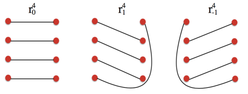
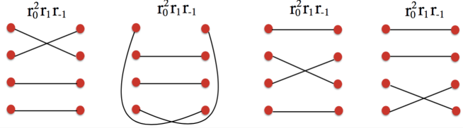
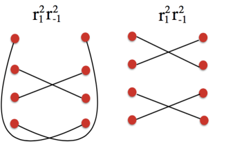
Figure 2: All contributing graphs for $k=1$, $n=4$. In this case the simple addition of individual contributions reproduces the exponential of the function (68).

A.2 The case $k=2$: excited state of two identical particles

For $k=2$ we have the formulae:

$$\mathcal{E}_{n}^{|\Psi_{2}(r_{1},r_{0},r_{-1})\rangle}=\log\left(\sum_{p=-2}^{2}\sum_{\sigma=\max(0,-np)}^{[\frac{n(2-p)}{2}]}A_{p,\sigma}r_{1}^{np+\sigma}r_{0}^{n(2-p)-2\sigma}r_{-1}^{\sigma}\right)\,,$$ (69)

where the sums have now been restricted only to non-vanishing contributions, and

$$A_{p,\sigma}=\sum_{\{k_{1},\ldots,k_{n}\}\in P_{n}(\sigma)}\prod_{j=1}^{n}\frac{2}{(p+k_{j})!(2-p-k_{j+1}-k_{j})!k_{j+1}!}\,,$$ (70)

therefore there are five possible values of $p$ to consider.

1. If $p=2$ the only partition of $\sigma$ that gives a non-vanishing coefficient is the partition where $k_{j}=0$ for all $j$. That is $\sigma=0$ and $A_{2,0}=1$ which gives the term $r_{1}^{2n}$.

2. If $p=1$ then the only partitions of $\sigma$ that give non-vanishing coefficients are those whose parts are either 0 or 1 and where there are no consecutive 1s. The latter condition means that $0\leq\sigma\leq\frac{n}{2}$ and

   $$A_{1,\sigma}=2^{n-\sigma}\times(\mathrm{number\,of\,such\,partitions})=2^{n-\sigma}Q_{\sigma}\,,$$ (71)

   where $Q_{\sigma}$ was defined in (65). This gives the terms

   $$\sum_{\sigma=0}^{[\frac{n}{2}]}2^{n-\sigma}Q_{\sigma}r_{1}^{n+\sigma}r_{0}^{n-2\sigma}r_{-1}^{\sigma}\,.$$ (72)

3. If $p=0$ the only partitions that give non-vanishing contributions are those that have parts which are either 0, 1 or 2 and which have no consecutive 2s and no consecutive 1s and 2s. There are many such partitions and challenge is to count them all and work out their contributions according to (70).

   The two simplest cases are the partition where all terms are 0s and the partition where all terms are 1s. In the first case $\sigma=0$ and $A_{0,0}=1$. This gives the contribution $r_{0}^{2n}$. In the second case we have that $\sigma=n$ and $A_{0,n}=2^{n}$ and this gives the term $2^{n}(r_{1}r_{-1})^{n}$. An additional partition corresponding to $\sigma=n$ is obtained when $n$ is even and every other term is either a 0 or a 2. There are two partitions of this type and when present they will give and additional contribution so that $A_{0,n}=2^{n}+2$, in agreement with the results we already knew from [32].

   More generally we can now consider all partitions including at least one 0 and 1s and 2s according to the constraints above. These correspond to $1\leq\sigma\leq n-1$.

   For $\sigma=1$ we have a single 1 and there are $n$ such partitions. The coefficient $A_{0,1}=\frac{2^{n}}{2^{n-2}}\times n$ and this gives the contribution $4nr_{0}^{2n-2}r_{1}r_{-1}$.

   For $\sigma=2$ we will now have partitions that contain either two 1s or a single 2 (with everything else being 0). There are $n$ partitions that contain a single 2 and they give a contribution to the coefficient $A_{0,2}$ which is given by $\frac{2^{n}}{2\times 2^{n-1}}\times n$. The partitions that contain two 1s can be divided into those where the 1s are consecutive and those where they are not. There are $n$ partitions that contain two consecutive 1s and their contribution to $A_{0,2}$ is $\frac{2^{n}}{2^{n-3}}\times n$. Finally the number of partitions that contain two non-consecutive ones is given by the coefficient $Q_{2}$ defined earlier and these give a contribution to $A_{0,2}$ which is given by $\frac{2^{n}}{2^{n-4}}\times Q_{2}$. So, overall

   $$A_{0,2}=\frac{2^{n}}{2^{n-4}}\times Q_{2}+\frac{2^{n}}{2^{n-3}}\times n+\frac{2^{n}}{2\times 2^{n-1}}\times n=8n(n-3)+8n+n=n(8n-15)\,,$$ (73)

   which gives the contribution $n(8n-15)r_{0}^{2n-4}(r_{1}r_{-1})^{2}$.

   For $\sigma=3$ we can have partitions that contain either three 1s or a 1 and a 2 that are not consecutive. The partitions that contain a 1 and a 2 that are not consecutive contribute

   $$\frac{2^{n}}{2\times 2^{n-4}\times 2}\times(\mathrm{number\,of\,such\,partitions})=4\times(2Q_{2})=4n(n-3).$$ (74)

   The partitions consisting of three 1s need to be divided into those where there are no consecutive 1s, those where two 1s are consecutive and those where the three 1s are consecutive. The partitions that have no consecutive 1s give a contribution

   $$\frac{2^{n}}{2^{n-6}}\times(\mathrm{number\,of\,such\,partitions})=64Q_{3}=\frac{32n(n-4)(n-5)}{3}.$$ (75)

   There are $n$ partitions where all three 1s are consecutive and they give a contribution

   $$\frac{2^{n}}{2^{n-4}}\times n=16n.$$ (76)

   Finally, the number of partitions where two 1s are consecutive and one is not is given by the product of $n$ ways of placing two consecutive 1s times $n-4$ ways of placing the remaining 1. This gives a contribution

   $$\frac{2^{n}}{2^{n-5}}\times{n(n-4)}={32n(n-4)}.$$ (77)

   So, the overall coefficient is

   $$A_{0,3}=4n(n-3)+\frac{32n(n-4)(n-5)}{3}+16n+{32n(n-4)}=\frac{4n}{3}(8n^{2}-45n+67).$$ (78)

   This gives the contribution $\frac{4n}{3}(8n^{2}-45n+67)r_{0}^{2n-6}(r_{1}r_{-1})^{3}$.

   One can proceed similarly to higher values of $\sigma$ and obtain increasingly complicated formulae for the coefficients as reported in Appendix B of [32]. However, there is no obvious pattern in $n$ emerging. Interestingly all coefficients $A_{0,\sigma}$ return integer values, even though this is also not obvious from the formulae.

4. If $p=-1$ we need partitions where all parts are at least 1, so the smallest allowed value of $\sigma$ is $\sigma=n$ corresponding to the partition into 1s. This gives $A_{-1,n}=2^{n}$ and corresponds to the term $2^{n}(r_{-1}r_{0})^{n}$. This is the “minimal” partition but there will be others. In fact, it is easy to argue that additional contributions will give rise to a very similar sum as (72) with the roles of $r_{1}$ and $r_{-1}$ exchanged:

   $$\sum_{\sigma=0}^{[\frac{n}{2}]}2^{n-\sigma}Q_{\sigma}r_{-1}^{n+\sigma}r_{0}^{n-2\sigma}r_{1}^{\sigma}\,,$$ (79)

5. If $p=-2$ we then need all parts of any contributing partition to be 2 or larger, for the first factorial in the denominator of (70) to be finite. All parts must be less or equal 2 for the second factorial to remain positive. This means only the partition consisting entirely of 2s will contribute. This corresponds to $\sigma=2n$ and $A_{-2,2n}=1$ and gives the contribution $r_{-1}^{2n}$.

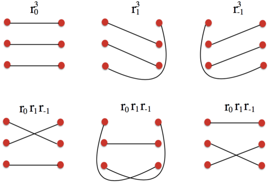
Figure 3: All contributing graphs for $k=1$, $n=3$. In this case the simple addition of individual contributions reproduces the exponential of the function (81).

The contributions discussed above can also be represented graphically. The basic building blocks are the same as for the $k=1$ case, however for $k=2$ every graph may be seen as a “superposition” of two $k=1$ graphs, and the counting of all possible (non-equivalent) such superpositions that are allowed under the rules set out in Fig. 1 quickly becomes involved. Let us consider, for simplicity, the case $n=3$. The expression for the replica logarithmic negativity is:

$$\mathcal{E}_{3}^{|\Psi_{2}(r_{1},r_{0},r_{-1})\rangle}=$$ (80)

$$\log(r_{0}^{6}+12r_{1}r_{-1}r_{0}(r_{1}^{3}+r_{-1}^{3}+r_{0}^{3})+8(r_{1}^{3}r_{0}^{3}+r_{-1}^{3}r_{0}^{3}+r_{1}^{3}r_{-1}^{3})+27r_{1}^{2}r_{-1}^{2}r^{2}+r_{1}^{6}+r_{-1}^{6})\,.$$

It is instructive to also report the case $k=1$, $n=3$:

$$\mathcal{E}_{3}^{|\Psi_{1}(r_{1},r_{0},r_{-1})\rangle}=\log(r_{0}^{3}+3r_{1}r_{-1}r_{0}+r_{1}^{3}+r_{-1}^{3})\,.$$ (81)

Although the expression for $k=1$ is much simpler than for $k=2$, we observe that all contributions to the $k=2$ case can be expressed (apart from the numerical coefficient) as products of two contributions to the $k=1$ case. Thus, whereas for $k=1$ we have a sum of 4 monomials, for $k=2$ we have a sum of 16 monomials. From the point of view of graphs, the case $k=1$, $n=3$ is extremely simple and is represented in Fig. 3. For $k=2$ we need to normalize each contribution by $\frac{1}{k^{n}}=\frac{1}{8}$ (representing the fact that each node can now be one of two excitations). For instance, the contribution $r_{0}^{6}$ in (80) can be seen as the result of adding all graphs in Fig. 4 and then dividing the result by 8.

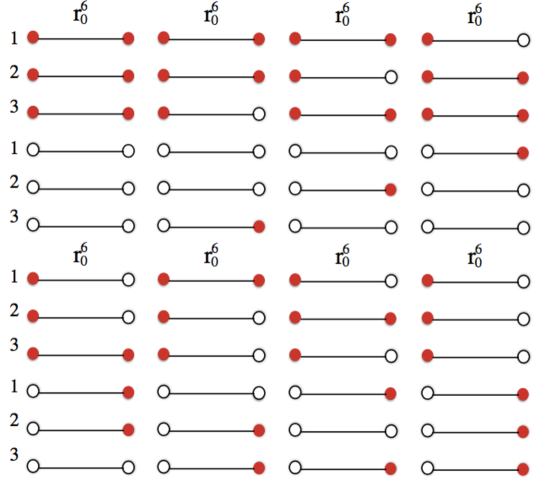
Figure 4: The contribution $r_{0}^{6}$ to the negativity for $k=2$, $n=3$. The differently coloured dots represent the two excitations. The numbers on the right hand side label the copies.

More interesting contributions correspond to terms such as $r_{1}^{2}r_{-1}^{2}r^{2}$ which is generated as $(r_{1}r_{-1}r_{0})^{2}$, that is as a “superposition” of any pair of graphs in the second row of Fig. 3. As in Fig. 4 we may have combinations of each of the three graphs with itself, producing $2^{3}$ possible graphs in each case. However, when combining two distinct graphs with each other, there are in fact $4^{3}$ possible combinations for each pairing. Since there are three possible pairings of two distinct graphs and three possible pairings of two identical graphs, this gives $3(2^{3}+4^{3})=216$ graphs and dividing again by $8$ this gives the coefficient 27 in (80).

Appendix B Recursion for replica negativity from graph partition function, $k=1$ case

In the case of a single particle excitation ($k=1$), it is possible to write a recursion formula for the graph partition function (2), and by solving it, express the replica logarithmic negativity as the analytic function derived by different means in [32]. Let us consider a restricted graph partition function

$$\tilde{p}_{1,n}(r_{1},r_{0},r_{-1})=\sum_{g\in{\tilde{\mathsf{G}}}_{1,n}}\prod_{\ell\in\{1,0,-1\}}r_{\ell}^{N_{\ell}(g)}\,,$$ (82)

summing only for graphs $\tilde{\mathsf{G}}_{1,n}$, where the vertices $V^{l,r}_{1,n+1}\neq V^{l,r}_{1,1}$ and $V^{l,r}_{1,0}\neq V^{l,r}_{1,n}$ are not identified. This restricts the possible edges of $\mathsf{E}_{1}$ and $\mathsf{E}_{-1}$. There is no edge in $\mathsf{E}_{1}$ attached to $V^{l}_{1,n}$ and no edge in $\mathsf{E}_{-1}$ attached to $V^{r}_{1,1}$. Moreover for every edge $(V^{l}_{1,j},V^{r}_{1,j+1})\in\mathsf{E}_{1}$ there is an edge $(V^{l}_{1,j+1},V^{r}_{1,j})\in\mathsf{E}_{-1}$, hence $N_{1}(g)=N_{-1}(g)$. This restriction give rise to the recursion relation

$$\tilde{p}_{1,n}(r_{1},r_{0},r_{-1})=r_{0}\tilde{p}_{1,n-1}(r_{1},r_{0},r_{-1})+r_{1}r_{-1}\tilde{p}_{1,n-2}(r_{1},r_{0},r_{-1})\,.$$ (83)

With the initial conditions $\tilde{p}_{1,0}(r_{1},r_{0},r_{-1})=1$ and $\tilde{p}_{1,1}(r_{1},r_{0},r_{-1})=r_{0}$ the solution of the recursion is

$$\tilde{p}_{1,n}(r_{1},r_{0},r_{-1})=\frac{\left(r_{0}+\sqrt{r_{0}^{2}+4r_{1}r_{-1}}\right)^{n+1}-\left(r_{0}-\sqrt{r_{0}^{2}+4r_{1}r_{-1}}\right)^{n+1}}{2^{n+1}\sqrt{r_{0}^{2}+4r_{1}r_{-1}}}\,.$$ (84)

The original graph partition function can be expressed with the help of the restricted graph partition function and two additional graphs where all the edges are either in $\mathsf{E}_{1}$ or $\mathsf{E}_{-1}$

$$p_{1,n}(r_{1},r_{0},r_{-1})=r_{1}^{n}+r_{-1}^{n}+\tilde{p}_{1,n}(r_{1},r_{0},r_{-1})+r_{1}r_{-1}\tilde{p}_{1,n-2}(r_{1},r_{0},r_{-1})\,.$$ (85)

Substituting (83) we arrive to the result

$$p_{1,n}(r_{1},r_{0},r_{-1})=r_{1}^{n}+r_{-1}^{n}+\left(\frac{r_{0}+\sqrt{r_{0}^{2}+4r_{1}r_{-1}}}{2}\right)^{n}+\left(\frac{r_{0}-\sqrt{r_{0}^{2}+4r_{1}r_{-1}}}{2}\right)^{n}\,,$$ (86)

that is the expression for $\exp\big{[}\mathcal{E}_{n}^{1}\big{]}$ derived in [32] where each term in the expression above is identified with a non-vanishing eigenvalue of the partially transposed reduced density matrix of the corresponding qubit state. From this formula, the analytic continuation $m\rightarrow 1/2$ for $n=2m$ also follows naturally.

References

- [1] C. H. Bennett, H. J. Bernstein, S. Popescu, and B. Schumacher, Concentrating partial entanglement by local operations, Phys. Rev. A53, 2046–2052 (1996).
- [2] K. Audenaert, J. Eisert, M. B. Plenio, and R. F. Werner, Entanglement properties of the harmonic chain, Phys. Rev. A66, 042327 (2002).
- [3] K. Życzkowski, P. Horodecki, A. Sanpera, and M. Lewenstein, Volume of the set of separable states, Phys. Rev. A 58, 883–892 (1998).
- [4] J. Eisert, Entanglement in quantum information theory (PhD Thesis), quant-ph/0610253 (2006).
- [5] M. B. Plenio, Logarithmic Negativity: A Full Entanglement Monotone That is not Convex, Phys. Rev. Lett. 95, 090503 (2005).
- [6] M. B. Plenio, Erratum: Logarithmic Negativity: A Full Entanglement Monotone That Is not Convex, Phys. Rev. Lett. 95, 119902 (2005).
- [7] G. Vidal and R. F. Werner, Computable measure of entanglement, Phys. Rev. A65, 032314 (2002).
- [8] C. J. Callan and F. Wilczek, On geometric entropy, Phys. Lett. B333, 55–61 (1994).
- [9] C. Holzhey, F. Larsen, and F. Wilczek, Geometric and renormalized entropy in conformal field theory, Nucl. Phys. B424, 443–467 (1994).
- [10] G. Vidal, J. I. Latorre, E. Rico, and A. Kitaev, Entanglement in quantum critical phenomena, Phys. Rev. Lett. 90, 227902 (2003).
- [11] J. I. Latorre, E. Rico, and G. Vidal, Ground state entanglement in quantum spin chains, Quant. Inf. Comput. 4, 48–92 (2004).
- [12] B.-Q. Jin and V. Korepin, Quantum spin chain, Toeplitz determinants and Fisher-Hartwig conjecture, J. Stat. Phys. 116, 79–95 (2004).
- [13] P. Calabrese and J. L. Cardy, Entanglement entropy and quantum field theory, J. Stat. Mech. 0406, P002 (2004).
- [14] J. L. Cardy, O. A. Castro Alvaredo and B. Doyon, “Form factors of branch-point twist fields in quantum integrable models and entanglement entropy”, J. Stat. Phys. 130, 129 (2008).
- [15] B. Doyon, Bi-partite entanglement entropy in massive two-dimensional quantum field theory, Phys. Rev. Lett. 102, 031602 (2009).
- [16] O. A. Castro-Alvaredo and B. Doyon, Entanglement entropy of highly degenerate states and fractal dimensions, Phys. Rev. Lett. 108, 120401 (2012).
- [17] P. Calabrese, J. Cardy, and E. Tonni, Entanglement entropy of two disjoint intervals in conformal field theory, J. Stat. Mech. 2009(11), P11001 (2009).
- [18] D. Bianchini, O. Castro-Alvaredo, B. Doyon, E. Levi, and F. Ravanini, Entanglement entropy of non-unitary conformal field theory, J.Phys. A48, 04FT01 (2015).
- [19] F. C. Alcaraz, M. I. Berganza, and G. Sierra, Entanglement of low-energy excitations in Conformal Field Theory, Phys. Rev. Lett. 106, 201601 (2011).
- [20] M. I. Berganza, F. C. Alcaraz, and G. Sierra, Entanglement of excited states in critical spin chains, J. Stat. Mech. 2012(01), P01016 (2012).
- [21] P. Calabrese, J. Cardy, and E. Tonni, Entanglement negativity in quantum field theory, Phys. Rev. Lett. 109, 130502 (2012).
- [22] P. Calabrese, J. Cardy, and E. Tonni, Entanglement negativity in extended systems: A field theoretical approach, J. Stat. Mech. 1302, P02008 (2013).
- [23] O. Blondeau-Fournier, O. Castro-Alvaredo, and B. Doyon, Universal scaling of the logarithmic negativity in massive quantum field theory, J. Phys. A49(12), 125401 (2016).
- [24] L. Amico, R. Fazio, A. Osterloh, and V. Vedral, Entanglement in many-body systems, Rev. Mod. Phys. 80, 517–576 (2008).
- [25] P. Calabrese, J. Cardy, and B. Doyon (ed), Entanglement entropy in extended quantum systems, J. Phys. A42, 500301 (2009).
- [26] J. Eisert, M. Cramer, and M. B. Plenio, Colloquium: Area laws for the entanglement entropy, Rev. Mod. Phys. 82, 277–306 (2010).
- [27] V. Knizhnik, Analytic fields on Riemann surfaces. II, Comm. Math. Phys. 112(4), 567–590 (1987).
- [28] L. Dixon, D. Friedan, E. Martinec, and S. Shenker, The conformal field theory of orbifolds, Nuclear Physics B 282, 13–73 (1987).
- [29] O. A. Castro-Alvaredo and B. Doyon, Permutation operators, entanglement entropy, and the XXZ spin chain in the limit , J. Stat. Mech. 1102, P02001 (2011).
- [30] O. A. Castro-Alvaredo, C. De Fazio, B. Doyon, and I. M. Szécsényi, Entanglement Content of Quasiparticle Excitations, Phys. Rev. Lett. 121, 170602 (2018).
- [31] O. A. Castro-Alvaredo, C. De Fazio, B. Doyon, and I. M. Szécsényi, Entanglement content of quantum particle excitations. Part I. Free field theory, JHEP 2018(10), 39 (2018).
- [32] O. A. Castro-Alvaredo, C. De Fazio, B. Doyon, and I. M. Szécsényi, Entanglement Content of Quantum Particle Excitations II. Disconnected Regions and Logarithmic Negativity, arXiv:1904.01035 (2019).
- [33] B. Pozsgay and G. Takacs, Form-factors in finite volume I: Form-factor bootstrap and truncated conformal space, Nucl. Phys. B788, 167–208 (2008).
- [34] B. Pozsgay and G. Takacs, Form factors in finite volume. II. Disconnected terms and finite temperature correlators, Nucl. Phys. B788, 209–251 (2008).
- [35] F. H. L. Essler and M. Fagotti, Quench dynamics and relaxation in isolated integrable quantum spin chains, J. Stat. Mech. 2016(6), 064002 (2016).
- [36] B. Doyon, Finite-temperature form factors in the Majorana theory, J. Stat. Mech. 2005, P11006 (2005).
- [37] B. Doyon, Finite-temperature form factors: a review, SIGMA 3, 011 (2007).
- [38] Y. Chen and B. Doyon, Form Factors in Equilibrium and Non-Equilibrium Mixed States of the Ising Model, J. Stat. Mech. 2014, P09021 (2014)