DDM: Fast Near-Optimal Multi-Robot Path Planning using Diversified-Path
and Optimal Sub-Problem Solution Database Heuristics

Abstract

We propose a novel centralized and decoupled algorithm, DDM, for solving multi-robot path planning problems in grid graphs, targeting on-demand and automated warehouse-like settings. Two settings are studied: a traditional one whose objective is to move a set of robots from their respective initial vertices to the goal vertices as quickly as possible, and a dynamic one which requires frequent re-planning to accommodate for goal configuration adjustments. Among other techniques, DDM is mainly enabled through exploiting two innovative heuristics: path diversification and optimal sub-problem solution databases. The two heuristics attack two distinct phases of a decoupling-based planner: while path diversification allows the more effective use of the entire workspace for robot travel, optimal sub-problem solution databases facilitate the fast resolution of local path conflicts. Extensive evaluation demonstrates that DDM achieves high levels of scalability and high levels of solution optimality.

I Introduction

Labeled optimal multi-robot path planning (MPP) problems, despite their high associated computational complexity [1], have been actively studied for decades due to the problems' extensive applications. The general task is to efficiently plan high-quality, collision-free paths to route a set of robots from an initial configuration to a goal configuration. Traditionally, the focus of studies on MPP is mainly with one-shot problems where the initial and goal configurations are pre-specified, and both are equal in cardinality to the number of the robots. More recently, an alternative dynamic formulation has started to attract more attention due to its real-world relevance [2]. A dynamic instance keeps assigning new goals to robots that already reached their current goals, thus requiring algorithms that can actively re-plan the paths to accommodate adjustments of goal configuration.

In this paper, we propose the DDM (Diversified-path Database-driven Multi-robot Path Planning) algorithm, capable of quickly computing near-optimal solutions to large-scale labeled MPPs, under both one-shot and dynamic settings on grid graphs. At a high-level, adapting the classic and effective decoupled planning paradigm [3, 4, 5, 6, 7], DDM first generates a shortest path between each pair of start and goal vertices and then resolves local conflicts among the initial paths. In generating the initial paths, a path diversification heuristic is introduced that attempts to make the path ensemble use all graph vertices in a balanced manner, which minimizes the chance that many robots aggregate in certain local areas, causing unwanted congestion. Then, in resolving path conflicts, we observe that most conflicts can be resolved in a local $2\times 3$ or $3\times 3$ area. Based on the observation, a second novel heuristic is introduced which builds a min-makespan solution database for all $2\times 3$ and $3\times 3$ sub-problems, and ensures quick local conflict resolution via database retrievals. Together, the two heuristics produce simultaneous improvement on both computational efficiency and solution optimality in terms of computing near-optimal solutions under practical settings, as compared with state-of-the-art methods, e.g., [8]. For example, our algorithm can compute $1.x$ optimal solutions for a few hundreds of robots on a $60\times 60$ grid with $10\%$ obstacles in under a second.

Related Work. MPP has been actively studied for many decades [9, 3, 10, 11], which is perhaps mainly due to its hardness and simultaneously, its practical importance. Both one-shot and dynamic MPP formulations find applications in a wide range of domains including evacuation [12], formation [13, 14], localization [15], microdroplet manipulation [16], object transportation [17], search and rescue [18], human robot interaction [19], and large-scale warehouse automation [20, 2], to list a few. MPP is known as Multi-Agent Pathfinding (MAPF) [21].

In the past decade, significant progress has been made on solving one-shot MPP problems. Optimal and sub-optimal solvers are achieved through reduction to other problems, e.g., SAT [22], answer set programming [23], and network flow [8]. Decoupled approaches [3], which first compute independent paths and then try to avoid collision afterward, are also popular. Commonly found decoupled approaches in a graph-based setting include independence detection [24], sub-dimensional expansion [25] and conflict-based search [26, 27]. Similar to our approach, there is a decoupled algorithm [28] which uses online calculations over local graph structures to handle path interactions. However, [28] only explored simple local interactions without much consideration to optimality. There also exists prioritized methods [6, 5, 29, 7] and a divide-and-conquer approach [30] which achieve decent scalability but at the cost of either completeness or optimality. Some anytime algorithms [31] are proposed to quickly find a feasible solution and then improve it. A learning-assisted approach [32] has recently been developed to automatically pick the algorithm that is likely to perform well on a given MPP task.

Dynamic MPP with new goals appearing over time, although not as extensively studied as its one-shot counterpart, has started to receive more attention. The problem is particularly applicable to automated warehouse systems [2]. Recent work has focused on the dynamic warehouse MPP setup, pursuing both better planning algorithms [33] and robust execution schedules [34]. Prioritized planning method with a flexible priority sequence has also been developed [35].

MPP is widely studied from many other perspectives. As such, our literature coverage here is necessarily limited; readers are referred to [36, 37, 38, 39, 40, 41, 42, 43] for some additional algorithmic developments on MPP under unlabeled (i.e., robots are indistinguishable), partially labeled, and continuous settings.

The topic of path diversification has been explored under both single and multi-robot settings. For single robot exploring a domain with many obstacles, obtaining a path ensemble can increase the chance of succeeding in finding a longer horizon plan [44, 45]. Similar to what we observe in the current study, path diversity is just one of the relevant factors affecting search success [46]. Survivability is also examined under a probabilistic framework for multi-robot systems [47]. In a similar context, a heuristic based on path conflicts expediates the solution process of an MPP algorithm [48].

Finally, the use of a sub-problem solution database trades off between offline and online computation, which is a general principle that finds frequent applications in robotics, e.g., [49, 50]. Relating to MPP, a similar technique called pattern database has been used in solving large $(n^{2}-1)$-puzzles [51, 52], as well as problems like Sokoban [53].

Main Contributions. This work brings three main contributions. First, based on the insight that decoupled MPP solvers tend to generate individual paths that aggregate in certain local areas (e.g., center of the workspace), we introduce path diversification heuristics that make more effective uses of the entire workspace. Second, the $2\times 3$ and $3\times 3$ sub-problem optimal solution databases, constructed one-time-only for resolving local path conflicts, bring significant on-line computational savings. Lastly, the first two main contributions jointly yield the DDM algorithm, which is effective not only for one-shot settings but also for dynamic MPP problems, as demonstrated through our extensive evaluation efforts.

Scope. We explicitly point out that DDM targets structured warehouse-like environments. As such, DDM is not suitable for MPPs with narrow passages, which remains challenging to be effectively solved. The current work focuses on synchronous path generation and does not address the equally important path execution aspects. Nevertheless, DDM can be readily combined with path execution approaches, e.g., [34], to form a complete planning and execution pipeline.

Organization. In Section II, we formally define both the one-shot and dynamic MPP formulations, and introduce assumptions. In Section III, we provide an overview of DDM. In Section IV and Section V, we describe the path diversification heuristics and the sub-problem solution database, respectively. In Section VI, we provide evaluation results of DDM. We conclude in Section VII.

II Preliminaries

II-A One-shot Multi-Robot Path Planning

Consider $n$ robots in an undirected grid graph $G(V,E)$. Given integers $w$ and $h$ as the width and height of the grid, we define the vertex set of $G$ as $V\subseteq\{(i,j)|1\leq i\leq w,1\leq j\leq h\}$; the elements not in $V$ are considered as static obstacles. Following the traditional $4$-way connectivity rule, for each vertex $(i,j)\in V$, its neighborhood is $N(i)=\{(i+1,j),(i-1,j),(i,j+1),(i,j-1)\}\cap V$. For a robot $i$ with initial and goal vertices $x^{I}_{i},x^{G}_{i}\in V$, a path is defined as a sequence of $T+1$ vertices $P_{i}=(p^{0}_{i},\dots,p^{T}_{i})$ satisfying: (i) $p^{0}_{i}=x^{I}_{i}$; (ii) $p^{T}_{i}=x^{G}_{i}$; (iii) $\forall 1\leq t\leq T$, $p^{t-1}_{i}=p^{t}_{i}$ or $p^{t-1}_{i}\in N(p^{t}_{i})$. Denoting the joint initial and goal configurations of the robots as $X^{I}=\{x_{1}^{I},\dots,x_{n}^{I}\}\subseteq V$ and $X^{G}=\{x_{1}^{G},\dots,x_{n}^{G}\}\subseteq V$, the path set of all the robots is then $\mathcal{P}=\{P_{1},\dots,P_{n}\}$.

For $\mathcal{P}$ to be collision-free, $\forall 1\leq t\leq T$, $P_{i},P_{j}\in\mathcal{P}$ must satisfy: (i) $p_{i}^{t}\neq p_{j}^{t}$ (no conflicts on vertices); (ii) $(p_{i}^{t-1},p_{i}^{t})\neq(p_{j}^{t},p_{j}^{t-1})$ (no ``head-to-head'' collisions on edges).

An optimal solution minimizes the makespan $T$, which is the time for all the robots to reach the goal vertices.

Problem 1.

Time-optimal Multi-robot Path Planning (MPP). Given $\langle G,X^{I},X^{G}\rangle$, find a collision-free path set $\mathcal{P}$ that routes the robots from $X^{I}$ to $X^{G}$ and minimizes $T$.

II-B Dynamic Multi-Robot Path Planning

The dynamic MPP formulation inherits most of one-shot MPP's structure, but with a few key differences. First, a robot $i$ will be assigned a new goal vertex when reaching its current goal $x^{G}_{i}$. Such a new goal is sampled from $V\backslash X^{G}$ using a certain distribution. Note that $X^{G}$ is continuously updated as new goals are assigned to the robots. Second, the optimization criteria is changed since the problem has no specific end state. In this paper, we maximize system throughput, which is the average number of goal arrivals in a unit of time.

Problem 2.

Dynamic Multi-robot Path Planning (DMP). Given $\langle G,X^{I},X^{G}\rangle$, route the robots in $G$, accommodate for changes in $X^{G}$, and maximize the system throughput.

II-C Assumptions on the Graph Structure

In this paper, we assume that the graph $G$ does not contain narrow passages, and the width of a passage in $G$ is at least $k\geq 2$. Formally speaking, we define $G$ as a low resolution graph: given $k$ as the narrowest passage width, there exists a bijection between the set of all grid Graphs $\mathcal{G}$ to the set of all low resolution graphs $\mathcal{G}_{\text{low}}^{k}$: $\mathcal{G}\rightarrow\mathcal{G}_{\text{low}}^{k},G(V,E)\mapsto G_{\text{low}}^{k}(V_{\text{low}}^{k},E_{\text{low}}^{k})$, where $V_{\text{low}}^{k}=\{(ki+x,kj+y)\mid\forall(i,j)\in V,x,y\in\{0,\dots,k-1\}\}$. A low-resolution graph example is provided in Fig. 1. By the definition, $k=2$ and $k=3$ are sufficient to ensure that all vertices in $G$ are contained in some $2\times 3$ or $3\times 3$ sub-graphs, respectively. The restriction on low-resolution graphs effectively prevents environments with narrow passages and mimics typical warehouse environments [2].

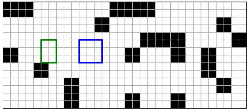
Figure 1: A $k=2$ low-resolution graph with $20\%$ obstacles. The white cells are vertices, and the black cells are obstacles. The green and blue rectangles visualize a $2\times 3$ and a $3\times 3$ sub-graph.

An essential component of our approach is the routing of robots inside some obstacle-free $2\times 3$ and $3\times 3$ sub-graphs. Examples of these sub-graphs are provided in Fig. 1. With the problem setup introduced in Section II-A, an MPP sub-problem in such a local sub-graph is always feasible [30], even when the sub-graph is fully occupied by robots.

Since DDM pipeline remains the same when using $2\times 3$ or $3\times 3$ sub-graphs, in the following sections we only use the $3\times 3$ sub-graph structure to introduce DDM.

III Overview of the DDM Algorithm

DDM follows the decoupled paradigm and first creates a shortest path for each robot from its initial vertex to goal vertex, ignoring other robots. Then, a simulated execution is carried out. As conflicts are detected, they are resolved within local sub-graphs. An illustration of the DDM pipeline is provided in Fig. 2. Although DDM is described as a centralized method, the conflict resolution phase can be readily decentralized. This is especially applicable to DMP: after the initial paths are acquired, collision avoidance can be implemented locally; during the path execution stage, any robot may change its desired path without causing a system failure since conflict resolution is performed on the fly.

\begin{overpic}[keepaspectratio,width=429.28616pt]{algorithm-pipeline-eps-converted-to.pdf} \footnotesize\put(13.55,20.5){(a)} \put(48.0,20.5){(b)} \put(82.0,20.5){(c)} \put(13.55,-2.5){(d)} \put(48.0,-2.5){(e)} \put(82.0,-2.5){(f)} \end{overpic}

Figure 2: Illustration of the DDM solution pipeline. (a) In a $5\times 3$ graph, the initial configuration of $3$ robots are visualized using blue, orange, and green disks. (b) The goal configuration. (c) The individual paths between each initial and goal vertex pairs are visualized using arrowed lines. (d) After simulating the individual paths for one time step, we find a collision in the next time step between the blue and orange robots. At this time, a local $3\times 3$ sub-graph is assigned to these two robots to resolve the conflict. The boundary of the sub-graph is highlighted in red. (e) The paths are updated using the $3\times 3$ solution. The robots are able to execute their new paths and get to the goal configuration without colliding with each other. (f) Alternative initial paths that are collision-free, which can be generated by using the path diversification heuristics.

Algorithm 1 describes DDM. In line 1, two structures are initialized: $X^{C}$ which keeps track of robots'current locations, and $\mathcal{G}_{3\times 3}$ which keeps a record of currently occupied $3\times 3$ sub-graphs used for collision avoidance.

Then, in line 1, DDM plans a shortest path from $x^{I}_{i}$ to $x^{G}_{i}$ for each robot $i$, without considering any interactions with the other robots. The detailed initial path generation process and its optimization techniques (i.e. the path diversification heuristics) are discussed in Section IV.

After the initial paths are acquired, DDM starts to carry out a simulated execution of these paths and resolves the conflicts between them. At the beginning of each simulation time step, DDM first checks whether collisions will occur if the robots all move along their planned paths (line 1–1). If no collision is detected, the collision avoidance procedures are skipped and the pipeline enters the execution stage (line 1–1).

1 $X^{C}\leftarrow X^{I}$, $\mathcal{G}_{3\times 3}\leftarrow\varnothing$

2 $\mathcal{P}_{\text{planned}}=\{P_{1},\dots,P_{n}\}\leftarrow$ GetPaths($G,X^{I},X^{G}$)

3 while $X^{C}\neq X^{G}$ do

4       $X^{N}\leftarrow$ GetNextStep($\mathcal{P}_{\text{planned}}$)

5       for $(i,j)\in$ CollidingRobotPairs($X^{C},X^{N}$) do

6             if $G_{3\times 3}\leftarrow$ FindSubGraph($G,X^{C},i,j,\mathcal{G}_{3\times 3}$) then

7                   $R\leftarrow\{i\,|\,x_{i}^{C}\in G_{3\times 3},\forall x_{i}^{C}\in X^{C}\}$

8                   $X^{I}_{3\times 3}\leftarrow\{x^{C}_{i}\,|\,i\in R\}$

9                   $X^{G}_{3\times 3}\leftarrow$ TempGoals($G_{3\times 3},R,\mathcal{P}_{\text{planned}}$)

10                   $\mathcal{P}_{\text{planned}}\leftarrow$ CheckDatabase($X^{I}_{3\times 3},X^{G}_{3\times 3}$)

11                   $\mathcal{G}_{3\times 3}\leftarrow\mathcal{G}_{3\times 3}\cup\{G_{3\times 3}$}

12                  

13            

14      $X^{C},\mathcal{P}_{\text{planned}}\leftarrow$ Simulate3x3Paths($X^{C},\mathcal{P}_{\text{planned}},\mathcal{G}_{3\times 3}$)

15       $X^{C},\mathcal{P}_{\text{planned}}\leftarrow$ SimulateOtherPaths($X^{C},\mathcal{P}_{\text{planned}}$)

16       $\mathcal{G}_{3\times 3}\leftarrow$ RemoveOutdatedSubGraphs($\mathcal{G}_{3\times 3}$)

17      

Algorithm 1 Centralized DDM for one-shot MPP

When collisions occur, DDM enters the collision avoidance stage (line 1–1). Here, whenever we iterate through robots, we give robots further away from their goal configurations a higher priority for the potential decrease of global makespan.

In line 1, we iterate through all the pairs of conflicting robots and for each pair of them, DDM first attempts to find an obstacle-free $3\times 3$ sub-graph which meets two requirements: (i) it contains both conflicting robots. (ii) it does not overlap with currently occupied $3\times 3$ graphs in $\mathcal{G}_{3\times 3}$. For requirement (i), when $G$ is obstacle-free, we can always find a $3\times 3$ graph that covers the colliding robots. Examples of such $3\times 3$ sub-graphs for all collision types are provided in Fig. 3(a-d). Note that since the $3\times 3$ sub-graphs shown in the sub-figures are not the only choices, when $G$ is a $k=3$ low-resolution graph, we can still find $3\times 3$ sub-graphs that meet requirement (i), except for the only outlier case shown in Fig. 3(e). In this case, we postpone the conflict by letting one robot wait and the other robot move. After one step of simulation, a $3\times 3$ graph satisfies requirement (i) will be available (see Fig. 3(f)). Note that a $3\times 3$ sub-graph satisfies requirement (i) may not meet requirement (ii). If we cannot find a $3\times 3$ graph that satisfies both requirements, we skip this pair of conflicting robots and start to process the next pair.

\begin{overpic}[keepaspectratio,width=429.28616pt]{collision-types-eps-converted-to.pdf} \footnotesize\put(11.7,29.2){(a)} \put(48.0,29.2){(b)} \put(84.5,29.2){(c)} \put(11.7,-3.5){(d)} \put(48.0,-3.5){(e)} \put(84.5,-3.5){(f)} \end{overpic}

Figure 3: (a–d) All types of collisions, including collisions on a vertex and head-to-head collisions on an edge, can be contained in some $3\times 3$ graphs (drawn in red). (e) The only scenario that we cannot find a $3\times 3$ sub-graph due to the black obstacle. (f) We can find a $3\times 3$ graph for the scenario in sub-figure (e) by postponing one robot's move.

If a $3\times 3$ sub-graph $G_{3\times 3}$ is acquired, in line 1, DDM locates all the robots that are currently inside $G_{3\times 3}$, whose paths will be affected by the conflict resolution process. DDM then assigns temporary goal configurations to all these robots (line 1) and route them inside $G_{3\times 3}$ by looking for the solution in the database (line 1). For the temporary goal assignment, we iterate through the affected robots and for each robot, we inspect its desired path backwards (i.e., from the goal to the robot's current location) and check if a vertex in the path also appears in $G_{3\times 3}$. We try to assign the first vertex appearing in $G_{3\times 3}$ as the robot's temporary goal. The purpose of such an assignment is to move robots closer to goals during collision avoidance. If the desired vertex is already assigned to another robot, we then opt for a random vertex in $G_{3\times 3}$ that is not assigned to other robots, since the temporary goals of different robots cannot be identical. In line 1, the min-makespan paths for routing these robots to the temporary goals are readily found in the database; further details is provided in Section V. The initial planned paths are updated according to the $G_{3\times 3}$ solution. Note that we might call GetPaths (in line 1) for a robot in case the original path and the $3\times 3$ solution cannot be simply concatenated due to a non-desirable temporary goal assignment. The final step of the collision avoidance stage is to put $G_{3\times 3}$ into $\mathcal{G}_{3\times 3}$ (line 1).

Recall that when constructing a $3\times 3$ graph in line 1, we require it not to overlap with other $3\times 3$ graphs already in use, i.e., the elements in $\mathcal{G}_{3\times 3}$. The requirement leaves some conflicts untreated, which are avoided in the following path execution process. In line 1, the robots in the current occupied $3\times 3$ graphs move first, since their paths are generated from the optimal solution database and are guaranteed to be collision-free. Then, in line 1, we move the other robots while avoiding collisions between them: first, we find all the robots that are moving into the sub-graphs in $\mathcal{G}_{3\times 3}$ and stop them, to avoid interruptions to the $3\times 3$ solutions' execution; next, we detect collisions in the current step, and recursively stop all the robots that are involved in these collisions. An illustration of this path execution process is provided in Fig. 4. Finally, in line 1, we remove elements from $\mathcal{G}_{3\times 3}$ if we finished executing the corresponding $3\times 3$ solutions. The untreated collisions mentioned in the beginning of this paragraph are either handled by the line 1, or by constructing a $3\times 3$ graph after the previous overlapping sub-graphs are removed from $\mathcal{G}_{3\times 3}$.

\begin{overpic}[keepaspectratio,width=429.28616pt]{execution-flow-eps-converted-to.pdf} \footnotesize\end{overpic}

Figure 4: Executing the planned paths which do not belong to $3\times 3$ sub-graph solutions. The red regions are the $3\times 3$ regions currently in $\mathcal{G}_{3\times 3}$; robots in these regions are omitted. The remaining robots are visualized using blue and gray disks, with arrows indicating the desired next time step moves. A blue disk implies that the robot is permitted to move, while a gray disk implies that the robot will stay still. The robots at top-right are stopped since one of them is trying to move into a sub-graph in $\mathcal{G}_{3\times 3}$. The robots at top-left and bottom are stopped due to collisions. We note that the figure is only for illustrating purposes and do not reflect actual cases.

The performance of DDM directly relates to the efficiency of the collision avoidance process, which is in turn influenced by the total number of path conflicts and the time to resolve a conflict. In the next two sections, we introduce optimization techniques including path diversification heuristics and the sub-graph solution database. These techniques enable DDM to achieve high levels of scalability and solution quality.

IV Path Diversification Heuristics

When individual paths are generated without care, their footprint tends to aggregate on portions of the graph environment, leading to higher chances for path conflicts. To alleviate this issue, multiple heuristics are attempted in this work. In the case where the graph is obstacle-free, we can reduce collisions by letting the robots go around the center. For graphs with arbitrary obstacles, we can reduce collisions by modifying the heuristic we used in the single robot path planning algorithm. As the number of potential collisions drops, DDM can generate solutions that are closer to optimal.

IV-A Graph without Obstacles

In an obstacle-free graph, the shortest path between two vertices is a set of axis-aligned moves according to the vertices' coordinate differences. For example, it takes $3$ steps along the x-axis and $2$ steps along the y-axis for a robot to move from 2D coordinate $(2,3)$ to $(5,5)$. Obtaining such a shortest path requires an ordering of these axis-aligned moves. Two ordering rules we studied are discussed as below.

Randomized Paths. This baseline ordering rule returns a randomized sequence of the axis-aligned moves. That is, for a path consisting of $i$ moves along the x-axis and $j$ moves along the y-axis, the moving sequence is uniformly randomly picked from $\binom{i+j}{i}$ possible orderings. As evidenced by Fig. 5(a), such a randomized sequence causes the graph center congested, and increases the initial paths' conflicts.

Path Diversification Using Single-Turn Paths. This heuristic moves a robot along one axis until the robot is aligned with the goal vertex, and then moves the robot along the other axis until it reaches the goal. There are two options when picking a single-turn path: depending on which axis to move along first, we can make the turning point closer or further away from the graph center. As indicated in Fig. 5(b), we can avoid congestion in the center of the graph by always choosing the turning point that is further away from the center. In Fig. 5(c), by mixing the selection of turning points that are closer and further away from the graph center, we can balance the vertex usage in the center and around the border.

\begin{overpic}[scale={0.27},angle={90}]{heatmap-no-obstacle-random-eps-converted-to.pdf} \footnotesize\put(45.0,-8.5){(a)} \end{overpic}

\begin{overpic}[scale={0.27},angle={90}]{heatmap-no-obstacle-single-turn-eps-converted-to.pdf} \footnotesize\put(45.0,-8.5){(b)} \end{overpic}

\begin{overpic}[scale={0.27},angle={90}]{heatmap-no-obstacle-combined-eps-converted-to.pdf} \footnotesize\put(45.0,-8.5){(c)} \end{overpic}

Figure 5: Comparison of different path-finding heuristics in an obstacle-free $48\times 27$ grid graph. We uniformly randomly sample $100000$ initial and goal vertex pairs and generate the initial paths using the studied rules. The color intensity of a cell reflects the number of time the cell is traversed by a path: the darker the color, the heavier the cell is utilized. (a) When using random paths, the center of the graph is congested. (b) When using single-turn paths, we can avoid congestion in the center. (c) A balance ($85\%,15\%$) between two types of single-turn paths avoids graph center under-utilization.

IV-B Graph with Obstacles

In a graph with obstacles, it is a natural choice to use the A* algorithm to generate the initial paths. The state space of the A* algorithm corresponds to the vertex set $V$.

The Manhattan Distance Heuristic. As a well-known traditional heuristic for path planning on a grid, the Manhattan distance sums up the absolute differences of two points' Cartesian coordinates. Given a goal vertex $(k,\ell)$, the heuristic value of a search state at vertex $(i,j)$ is calculated as

$$H_{\text{Manhattan}}[(i,j)]=|i-k|+|j-\ell|.$$

The Manhattan distance heuristic leads to extensive utilization of vertices around obstacles and congestion on some high-traffic lanes (see Fig. 6(a)).

Since the initial path planning is performed sequentially over the $n$ robots, a path generated later can avoid conflicts with earlier paths. In this work, we realize this concept using two innovative path diversification heuristics.

Path Diversification by Vertex Occupancy. We define the occupancy of a vertex as the number of paths traverse through the vertex. Denoting $\mathbb{N}_{0}$ as the set of all non-negative integers, we construct a map $O:V\to\mathbb{N}_{0}$ to actively track the occupancy of all vertices throughout the initial path generation process. At the beginning, for each $(i,j)\in V$, $O[(i,j)]=0$. Then, we sort the robots and generate initial paths for robots with goals further away (in terms of the Manhattan distance) from the initial vertices first. After each path is generated by the A* algorithm, $O$ is updated such that for each vertex $(i,j)$ in the path, $O[(i,j)]$ increments by $1$. The heuristic value for search state $(i,j)$ is calculated as

$$H_{\text{Occupancy}}[(i,j)]=H_{\text{Manhattan}}[(i,j)]+O[(i,j)]/n.$$

Here, the last term of the equation refers to the additional cost imposed by path intersections. A constant value $n$ (i.e. the number of robots) is used to balance between finding a shorter path and finding a path with less interference with the others. In practice, we notice that this constant value ensures path diversification while keeps the initial paths short.

Fig. 6(b) demonstrates the effect of the vertex occupancy heuristic on a graph with obstacles. Comparing the two sub-figures, we observe reduced congestion around obstacles and high-traffic lanes when using the path diversification heuristic.

Path Diversification by a State-Time Map. As an alternative path diversification heuristic, instead of just calculating vertex usage, we also take the time domain into account. Since there are generally two types of collisions (see Fig. 3(a)) between robots: on a vertex or head-to-head on an edge, we now store the state-time information in a map $S:(V\cup E,\mathbb{N}_{0})\to\mathbb{N}_{0}$, which specifies the number of times a vertex or an edge is used at a certain time step. Now, for an A* search state at vertex $(i,j)$ with cost-to-go value $t$, its state-time heuristic value is calculated as

$$H_{\text{StateTime}}[(i,j),t]= \,H_{\text{Manhattan}}[(i,j)]$$

$$+(S[(i,j),t] +S[(\textsc{Parent}(i,j),(i,j)),t])/n,$$

with the first term on the second line refers to path conflicts on vertices, and the second term refers to conflicts on edges.

\begin{overpic}[scale={0.425},angle={90}]{heatmap-with-obstacle-astar-eps-converted-to.pdf} \footnotesize\put(45.0,-6.0){(a)} \end{overpic}

\begin{overpic}[scale={0.425},angle={90}]{heatmap-with-obstacle-avoidance-eps-converted-to.pdf} \footnotesize\put(45.0,-6.0){(b)} \end{overpic}

Figure 6: Comparison of different path finding heuristics in a graph with obstacles visualized in black. Other visual elements are the same as the ones in Fig. 5. (a) Pure Manhattan distance heuristic. (b) Path diversification by vertex occupancy.

When comparing the vertex occupancy heuristic with the state-time heuristic, it is not hard to see that since the state-time heuristic takes the time domain into consideration, it generates initial path sets with less conflicts. However, due to the fact that the initial paths might be modified during the DDM simulated execution phase, as we will demonstrate in Section VI, the vertex occupancy heuristic provides overall better solutions in terms of makespan. This is as expected since the effect of the vertex occupancy heuristic is less likely to be affected by unsynchronized path execution.

V $2\times 3$ and $3\times 3$ Problem Solution Database

We now provide the details of the optimal sub-problem solution database, especially how the database is generated.

Generating the $2\times 3$ database and the $3\times 3$ database follow largely similar steps. Here, we use the case of $3\times 3$ database to illustrate the necessary computation, which requires a bit more technical trickeries than the $2\times 3$ case. Let $X_{n}$ be the set of all configurations of $n$ ($1\leq n\leq 9$) robots in a $3\times 3$ graph, bijections exist between the set of all problem instances, the set of all solutions, and all pairs of initial and goal combinations $X_{n}\times X_{n}$. The solution space has a size

$$\sum_{n=1}^{9}|X_{n}\times X_{n}|=\sum_{n=1}^{9}|X_{n}|^{2}=\sum_{n=1}^{9}(\binom{9}{n}n!)^{2}\approx 3\times 10^{11},$$

which is too large to compute and store. In this section, we introduce how this issue is resolved by exploiting symmetry.

Permutation Elimination. Instead of exploring all possible combinations of $X^{I}$ and $X^{G}$, for each problem instance recorded in the database, we always sort $X^{I}$. Note that we can still find the solution for an arbitrary pair of $X^{I}$ and $X^{G}$: we first apply a permutation $\pi$ to both $X^{I}$ and $X^{G}$, such that $\pi(X^{I})$ is sorted. Denoting $\mathcal{P}$ as the solution for $\pi(X^{I})$ and $\pi(X^{G})$ in the database, the solution for $X^{I}$ and $X^{G}$ is then $\pi^{-1}(\mathcal{P})$. More details are provided at the end of this section. The size of the $3\times 3$ database is now reduced to

$$\sum_{n=1}^{9}\binom{9}{n}|X_{n}|=\sum_{n=1}^{9}(\binom{9}{n}^{2}n!)\approx 1.7\times 10^{7}.$$

Group Actions. When generating the database, after we calculated a solution $\mathcal{P}$ for certain $X^{I}$, $X^{G}$, this solution can possibly be translated to the solutions for other related instances by taking the same action to $X^{I}$, $X^{G}$ and $\mathcal{P}$.

In this work, we explore two types of actions. The first one, based on rotational symmetry, is to rotate all the configurations by the same degree. After this rotation, the processed $\mathcal{P}$ becomes the solution for the rotated $X^{I}$, $X^{G}$. Denoting $r$ as rotating a configuration clockwise by $90$ degrees, the set of all possible rotations is then $\{1,r,r^{2},r^{3}\}$. Here, $1=r^{4}$, which is interpreted as rotating a configuration by $360$ degrees, has no effect.

The second action, based on mirror symmetry, is to flip a configuration by the vertical middle line of a $3\times 3$ graph. The set of flip actions is denoted as $\{1,f\}$.

Combining the two types of actions, we have

$$\{1,r,r^{2},r^{3}\}\times\{1,f\}=\{1,r,r^{2},r^{3},f,fr,fr^{2},fr^{3}\}.$$

Here, $fr^{2}$ is interpreted as flipping the configuration, and then rotate the flipped configuration clockwise by $180$ degrees.

With a set of calculated $X^{I}$, $X^{G}$, $\mathcal{P}$, applying each action in this set results in a new problem and the solution to it. Note that the group actions above already includes counter-clockwise rotations and other types of flipping. In Fig. 7, we show the result of applying these actions to a configuration.

\begin{overpic}[keepaspectratio,width=429.28616pt]{group-actions-eps-converted-to.pdf} \footnotesize\put(10.2,24.5){$1$} \put(36.0,24.5){$r$} \put(61.9,24.5){$r^{2}$} \put(87.6,24.5){$r^{3}$} \put(10.2,-3.5){$f$} \put(34.8,-3.5){$fr$} \put(60.0,-3.5){$fr^{2}$} \put(86.0,-3.5){$fr^{3}$} \end{overpic}

Figure 7: Using group actions, we can generate up to eight different configurations out of one configuration.

Moreover, $\mathcal{P}$ can be reversed to route the robots from $X^{G}$ to $X^{I}$. All in all, we can generate up to $16$ unique solutions out of the solution for a pair of $X^{I}$ and $X^{G}$ using this reversing process combined with group actions, which expedites the database generation process since we now only need to calculate around $1.1\times 10^{6}$ problem instances.

By permutation elimination and group actions, the computation time for obtaining the database is significantly reduced. Using an integer linear programming-based solver [8], generating the full $3\times 3$ solution database takes about six hours.

\begin{overpic}[keepaspectratio,width=65.04034pt]{3x3-eps-converted-to.pdf} \footnotesize\put(11.0,11.0){$0$} \put(43.0,11.0){$1$} \put(76.0,11.0){$2$} \put(11.0,43.0){$3$} \put(43.0,43.0){$4$} \put(76.0,43.0){$5$} \put(11.0,76.0){$6$} \put(43.0,76.0){$7$} \put(76.0,76.0){$8$} \end{overpic}  

Figure 8: An illustration of database lookup. As demonstrated in the left figure, we give each vertex in the $3\times 3$ graph a unique id. The example on the right is a database lookup for three robots. First, a permutation $\pi$ is applied to sort the initial configuration from $065$ to $056$; the goal configuration is updated accordingly. After the transition steps between the sorted initial and goal configurations are acquired from the database, a permutation $\pi^{-1}$ is applied to generate a solution for the original problem.

Database Lookup. When we run DDM, the database is pre-loaded into a C++ STL map, with key and value both string types. Here, the key is a composition of the initial and goal configurations, and the value indicates the min-makespan paths between the two configurations. For a database lookup, we first apply a permutation to both the initial and goal configurations so that the initial configuration is sorted. Then, we compile the configurations into a single string and lookup for the value for this key in the database. Finally, we translate the value string into the solution paths. We provide an example of database lookup in Fig. 8. Our database is light-weight and fast to query: the $3\times 3$ database uses 500MB disk storage, and takes 2GB memory when loaded into C++ STL map; the $2\times 3$ database is less than 300KB. Accessing $1000$ random keys sequentially takes less than one millisecond in total.

VI Simulation Result

In this section, we compare DDM with integer linear programming (ILP) [8] and Enhanced Conflict-Based Search (ECBS) [48] under the classic one-shot MPP setting. The methods compared are to the best of our knowledge some of the fastest (near-)optimal solvers for MPP. For ILP, we evaluated the original optimal version ILP Exact and a sub-optimal variant ILP $k$-way Split. For ECBS, we set its weight parameter $w=1.5$ since it seems to be a good balance between optimality and scalability in the original publication and from our observation. Besides MPP, we also tested DDM on the dynamic formulation DMP. All our experiments are performed on an Intel^® Core^TM i7-6900k CPU at $3.2$GHz. Each data point is an average over $30$ runs on randomly generated instances. Although we do not provide a theoretical completeness and optimality guarantee for DDM, the algorithm quickly solves all the problem instances we have tested, and provides near-optimal solutions.

We first examine a one-shot case on a $24\times 18$ grid without obstacles. The start and goal vertices are uniformly randomly sampled. The result is compiled in Fig. 9. Here, the $2\times 3$ entires only construct $2\times 3$ sub-graphs, and $3\times 3$ entry means a $3\times 3$ sub-problem is constructed whenever it is possible. The optimality ratio is calculated as the resulting makespan over the optimal makespan computed by ILP Exact. The comparison of computation time (the top sub-figure) shows that DDM is the fastest method, which is about one to two magnitudes faster than the compared approaches. In particular, $2\times 3$ SingleTurn is about $10^{4}$ times faster than ILP Exact and $60$ times faster than ECBS. At the same time, most of the DDM variants maintained $1.x$ optimality.

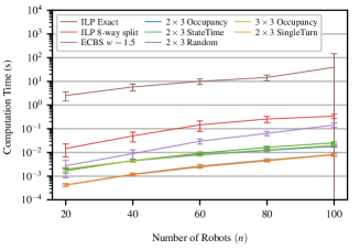
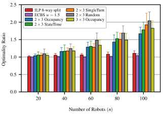
Figure 9: Average computation time (top sub-figure) and makespan (bottom sub-figure), and the standard deviations of algorithms on MPP tested in a $24\times 18$ obstacle-free grid, with varied number of robots. We use notation Random to indicate no path diversification heuristic is used.

The result suggests that using $2\times 3$ sub-graphs generates better solutions than using $3\times 3$ ones, which is due to $2\times 3$ graphs having a smaller footprint. Thus, interruptions to other robots is less likely. We hypothesized that resolving local conflicts using $3\times 3$ sub-graphs could help improve optimality; this turns out not to be the case in our tests. Nevertheless, for completeness, we include results on $3\times 3$ sub-graphs.

In a second evaluation, we switch to a $69\times 36$ warehouse-like environment (Fig. 10) with many blocks of static obstacles. For this case, between $50$ and $300$ robots are attempted. The evaluation results are shown in Fig. 11, which show similar performance trends as Fig. 9. Here, because ILP Exact can no longer finish each and every calculation in ten minutes, comparison on optimality is made with respect to an underestimated makespan which is calculated without considering robot-robot collisions. DDM provides more than $50$ times speed up without sacrificing much optimality.

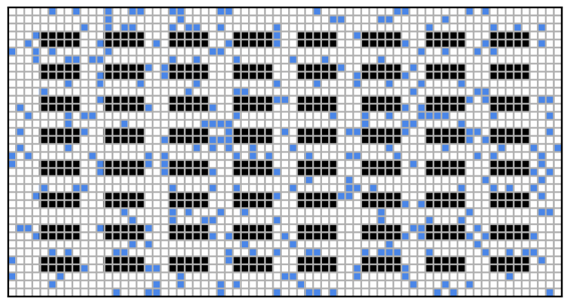
Figure 10: A $69\times 36$ warehouse-style workspace with $8$ row, $8$ column $5\times 2$ obstacle blocks. A random configuration of $300$ robots is colored in blue.

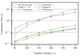
Figure 11: Evaluation results of MPP in a warehouse-style workspace.

Evident in the MPP results, DDM can handle the frequent re-planning request of a few hundreds of robots in large environments. We further compare the DDM variants in DMP and see how the benefits of heuristics are carried to the dynamic setting. Here, we do not involve other methods since the DMP formulation is relatively new and we could not locate comparable algorithms designed for DMP under a warehouse setting in the research literature. Our evaluation of DMP measures system throughput by the makespan for the robots to reach $10000$ uniformly randomly sampled goal configurations in total. Fig. 12 shows the evaluation results. The performance comparison between the DDM variants is consistent with the one-shot results. The experiment also shows an interesting trend: the total makespan initially drops quickly as the number of robots increases; as the number of robots keeps increasing, the total makespan then begins to get larger again. This makes intuitive sense because too many robots are expected to make routing harder in more complex environments. The optimal makespan is achieved at around $150$ and $300$ robots. Viewing this together with Fig. 11, we draw the conclusion that DDM achieves a much faster computation speed with minor loss on optimality.

All tests are repeated with varied grid sizes and obstacle percentages. The results, which are omitted due to space constraint, are consistent in all cases.

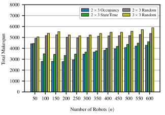
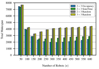
Figure 12: Evaluation results of DMP in (top) a $30\times 30$ low-resolution grid ($k=2$) with $10\%$ ($90$) obstacles, and (bottom) the warehouse-style workspace in Fig. 10.

A video of simulated DDM runs can be found at https://youtu.be/briO507tJiY.

VII Conclusion and Future Work

In this work, we developed a decoupled multi-robot path planning algorithm, DDM. With the proposed heuristics based on path diversification, which seeks to balance the use of graph vertices, and the employment of sub-problem solution databases for fast and optimal local conflict resolution, DDM is empirically shown to achieve significantly faster computational speed while producing high quality solutions, for both one-shot and dynamic problem settings.

In proposing DDM, our hope is to optimize the algorithm for the two main phases of a decoupled approach. While the initial iteration of DDM shows promising performance, in future work, we would like to apply the novel heuristics from DDM for solving multi-robot path planning problems beyond warehouse-like settings. In addition, improvements to these heuristics are possible. For example, we only attempted $2\times 3$ and $3\times 3$ solution databases; databases using other graphs might provide better performance. Also, tighter integration of the two heuristics may further boost performance.

References

- [1] J. Yu and S. M. LaValle, ``Structure and intractability of optimal multi-robot path planning on graphs,'' in Proceedings AAAI National Conference on Artificial Intelligence, 2013, pp. 1444–1449.
- [2] P. R. Wurman, R. D'Andrea, and M. Mountz, ``Coordinating hundreds of cooperative, autonomous vehicles in warehouses,'' AI Magazine, vol. 29, no. 1, pp. 9–19, 2008.
- [3] M. A. Erdmann and T. Lozano-Pérez, ``On multiple moving objects,'' in Proceedings IEEE International Conference on Robotics & Automation, 1986, pp. 1419–1424.
- [4] G. Sanchez and J.-C. Latombe, ``Using a prm planner to compare centralized and decoupled planning for multi-robot systems,'' in Robotics and Automation, 2002. Proceedings. ICRA'02. IEEE International Conference on, vol. 2. IEEE, 2002, pp. 2112–2119.
- [5] M. Bennewitz, W. Burgard, and S. Thrun, ``Finding and optimizing solvable priority schemes for decoupled path planning techniques for teams of mobile robots,'' Robotics and autonomous systems, vol. 41, no. 2, pp. 89–99, 2002.
- [6] J. van den Berg and M. Overmars, ``Prioritized motion planning for multiple robots,'' in Proceedings IEEE/RSJ International Conference on Intelligent Robots & Systems, 2005.
- [7] J. van den Berg, J. Snoeyink, M. Lin, and D. Manocha, ``Centralized path planning for multiple robots: Optimal decoupling into sequential plans,'' in Robotics: Science and Systems, 2009.
- [8] J. Yu and S. M. LaValle, ``Optimal multi-robot path planning on graphs: Complete algorithms and effective heuristics,'' IEEE Transactions on Robotics, vol. 32, no. 5, pp. 1163–1177, 2016.
- [9] O. Goldreich, ``Finding the shortest move-sequence in the graph-generalized 15-puzzle is NP-hard,'' 1984, laboratory for Computer Science, Massachusetts Institute of Technology, Unpublished manuscript.
- [10] S. M. LaValle and S. A. Hutchinson, ``Optimal motion planning for multiple robots having independent goals,'' IEEE Transactions on Robotics & Automation, vol. 14, no. 6, pp. 912–925, Dec. 1998.
- [11] Y. Guo and L. E. Parker, ``A distributed and optimal motion planning approach for multiple mobile robots,'' in Proceedings IEEE International Conference on Robotics & Automation, 2002, pp. 2612–2619.
- [12] S. Rodriguez and N. M. Amato, ``Behavior-based evacuation planning,'' in Proceedings IEEE International Conference on Robotics & Automation, 2010, pp. 350–355.
- [13] S. Poduri and G. S. Sukhatme, ``Constrained coverage for mobile sensor networks,'' in Proceedings IEEE International Conference on Robotics & Automation, 2004.
- [14] B. Smith, M. Egerstedt, and A. Howard, ``Automatic generation of persistent formations for multi-agent networks under range constraints,'' ACM/Springer Mobile Networks and Applications Journal, vol. 14, no. 3, pp. 322–335, June 2009.
- [15] D. Fox, W. Burgard, H. Kruppa, and S. Thrun, ``A probabilistic approach to collaborative multi-robot localization,'' Autonomous Robots, vol. 8, no. 3, pp. 325–344, June 2000.
- [16] E. J. Griffith and S. Akella, ``Coordinating multiple droplets in planar array digital microfluidic systems,'' International Journal of Robotics Research, vol. 24, no. 11, pp. 933–949, 2005.
- [17] D. Rus, B. Donald, and J. Jennings, ``Moving furniture with teams of autonomous robots,'' in Proceedings IEEE/RSJ International Conference on Intelligent Robots & Systems, 1995, pp. 235–242.
- [18] J. S. Jennings, G. Whelan, and W. F. Evans, ``Cooperative search and rescue with a team of mobile robots,'' in Proceedings IEEE International Conference on Robotics & Automation, 1997.
- [19] R. A. Knepper and D. Rus, ``Pedestrian-inspired sampling-based multi-robot collision avoidance,'' in 2012 IEEE RO-MAN: The 21st IEEE International Symposium on Robot and Human Interactive Communication. IEEE, 2012, pp. 94–100.
- [20] P. R. Wurman, R. D'Andrea, and M. Mountz, ``Coordinating hundreds of cooperative, autonomous vehicles in warehouses,'' in Proceedings of the 19th national conference on Innovative applications of artificial intelligence - Volume 2, ser. IAAI'07, 2007, pp. 1752–1759.
- [21] R. Stern, N. Sturtevant, A. Felner, S. Koenig, H. Ma, T. Walker, J. Li, D. Atzmon, L. Cohen, T. Kumar, et al., ``Multi-agent pathfinding: Definitions, variants, and benchmarks,'' arXiv preprint arXiv:1906.08291, 2019.
- [22] P. Surynek, ``Towards optimal cooperative path planning in hard setups through satisfiability solving,'' in Proceedings 12th Pacific Rim International Conference on Artificial Intelligence, 2012.
- [23] E. Erdem, D. G. Kisa, U. Öztok, and P. Schueller, ``A general formal framework for pathfinding problems with multiple agents.'' in AAAI, 2013.
- [24] T. Standley and R. Korf, ``Complete algorithms for cooperative pathfinding problems,'' in Proceedings International Joint Conference on Artificial Intelligence, 2011, pp. 668–673.
- [25] G. Wagner and H. Choset, ``Subdimensional expansion for multirobot path planning,'' Artificial Intelligence, vol. 219, pp. 1–24, 2015.
- [26] E. Boyarski, A. Felner, R. Stern, G. Sharon, O. Betzalel, D. Tolpin, and E. Shimony, ``Icbs: The improved conflict-based search algorithm for multi-agent pathfinding,'' in Eighth Annual Symposium on Combinatorial Search, 2015.
- [27] L. Cohen, T. Uras, T. Kumar, H. Xu, N. Ayanian, and S. Koenig, ``Improved bounded-suboptimal multi-agent path finding solvers,'' in International Joint Conference on Artificial Intelligence, 2016.
- [28] K.-H. C. Wang and A. Botea, ``Mapp: a scalable multi-agent path planning algorithm with tractability and completeness guarantees,'' Journal of Artificial Intelligence Research, vol. 42, pp. 55–90, 2011.
- [29] M. Saha and P. Isto, ``Multi-robot motion planning by incremental coordination,'' in 2006 IEEE/RSJ International Conference on Intelligent Robots and Systems. IEEE, 2006, pp. 5960–5963.
- [30] J. Yu, ``Constant factor time optimal multi-robot routing on high-dimensional grids in mostly sub-quadratic time,'' arXiv preprint arXiv:1801.10465, 2018.
- [31] K. Vedder and J. Biswas, ``X*: Anytime multiagent planning with bounded search,'' in Proceedings of the 18th International Conference on Autonomous Agents and MultiAgent Systems. International Foundation for Autonomous Agents and Multiagent Systems, 2019, pp. 2247–2249.
- [32] D. Sigurdson, V. Bulitko, S. Koenig, C. Hernandez, and W. Yeoh, ``Automatic algorithm selection in multi-agent pathfinding,'' arXiv preprint arXiv:1906.03992, 2019.
- [33] H. Ma, J. Li, T. Kumar, and S. Koenig, ``Lifelong multi-agent path finding for online pickup and delivery tasks,'' in Proceedings of the 16th Conference on Autonomous Agents and MultiAgent Systems. International Foundation for Autonomous Agents and Multiagent Systems, 2017, pp. 837–845.
- [34] W. Hoenig, S. Kiesel, A. Tinka, J. W. Durham, and N. Ayanian, ``Persistent and robust execution of mapf schedules in warehouses,'' IEEE Robotics and Automation Letters, 2019.
- [35] K. Okumura, M. Machida, X. Défago, and Y. Tamura, ``Priority inheritance with backtracking for iterative multi-agent path finding,'' arXiv preprint arXiv:1901.11282, 2019.
- [36] M. Turpin, K. Mohta, N. Michael, and V. Kumar, ``CAPT: Concurrent assignment and planning of trajectories for multiple robots,'' International Journal of Robotics Research, vol. 33, no. 1, pp. 98–112, 2014.
- [37] J. Yu and S. M. LaValle, ``Distance optimal formation control on graphs with a tight convergence time guarantee,'' in Proceedings IEEE Conference on Decision & Control, 2012, pp. 4023–4028.
- [38] K. Solovey and D. Halperin, ``-color multi-robot motion planning,'' in Proceedings Workshop on Algorithmic Foundations of Robotics, 2012.
- [39] J. van den Berg, M. C. Lin, and D. Manocha, ``Reciprocal velocity obstacles for real-time multi-agent navigation,'' in Proceedings IEEE International Conference on Robotics & Automation, 2008, pp. 1928–1935.
- [40] J. Snape, J. van den Berg, S. J. Guy, and D. Manocha, ``The hybrid reciprocal velocity obstacle,'' IEEE Transactions on Robotics, vol. 27, no. 4, pp. 696–706, 2011.
- [41] R. Chinta, S. D. Han, and J. Yu, ``Coordinating the motion of labeled discs with optimality guarantees under extreme density,'' in The 13th International Workshop on the Algorithmic Foundations of Robotics, 2018.
- [42] A. Adler, M. De Berg, D. Halperin, and K. Solovey, ``Efficient multi-robot motion planning for unlabeled discs in simple polygons,'' in Algorithmic Foundations of Robotics XI. Springer, 2015, pp. 1–17.
- [43] K. Solovey, J. Yu, O. Zamir, and D. Halperin, ``Motion planning for unlabeled discs with optimality guarantees,'' in Robotics: Science and Systems, 2015.
- [44] M. S. Branicky, R. A. Knepper, and J. J. Kuffner, ``Path and trajectory diversity: Theory and algorithms,'' in 2008 IEEE International Conference on Robotics and Automation. IEEE, 2008, pp. 1359–1364.
- [45] L. H. Erickson and S. M. LaValle, ``Survivability: Measuring and ensuring path diversity,'' in 2009 IEEE International Conference on Robotics and Automation. IEEE, 2009, pp. 2068–2073.
- [46] R. A. Knepper and M. T. Mason, ``Path diversity is only part of the problem,'' in Robotics and Automation, 2009. ICRA'09. IEEE International Conference on. IEEE, 2009, pp. 3224–3229.
- [47] Y.-H. Lyu, Y. Chen, and D. Balkcom, ``-survivability: Diversity and survival of expendable robots,'' IEEE Robotics and Automation Letters, vol. 1, no. 2, pp. 1164–1171, 2016.
- [48] M. Barer, G. Sharon, R. Stern, and A. Felner, ``Suboptimal variants of the conflict-based search algorithm for the multi-agent pathfinding problem,'' in Seventh Annual Symposium on Combinatorial Search, 2014.
- [49] R. Tedrake, ``Lqr-trees: Feedback motion planning on sparse randomized trees,'' 2009.
- [50] K. Hauser, ``Learning the problem-optimum map: Analysis and application to global optimization in robotics,'' IEEE Transactions on Robotics, vol. 33, no. 1, pp. 141–152, 2017.
- [51] A. Felner and A. Adler, ``Solving the 24 puzzle with instance dependent pattern databases,'' in International Symposium on Abstraction, Reformulation, and Approximation. Springer, 2005, pp. 248–260.
- [52] A. Felner, R. E. Korf, R. Meshulam, and R. C. Holte, ``Compressed pattern databases.'' J. Artif. Intell. Res.(JAIR), vol. 30, pp. 213–247, 2007.
- [53] A. G. Pereira, M. R. P. Ritt, and L. S. Buriol, ``Finding optimal solutions to sokoban using instance dependent pattern databases,'' in Sixth Annual Symposium on Combinatorial Search, 2013.