Online Convex Matrix Factorization with Representative Regions

Abstract

Matrix factorization (MF) is a versatile learning method that has found wide applications in various data-driven disciplines. Still, many MF algorithms do not adequately scale with the size of available datasets and/or lack interpretability. To improve the computational efficiency of the method, an online (streaming) MF algorithm was proposed in Mairal et al. [2010]. To enable data interpretability, a constrained version of MF, termed convex MF, was introduced in Ding et al. [2010]. In the latter work, the basis vectors are required to lie in the convex hull of the data samples, thereby ensuring that every basis can be interpreted as a weighted combination of data samples. No current algorithmic solutions for online convex MF are known as it is challenging to find adequate convex bases without having access to the complete dataset. We address both problems by proposing the first online convex MF algorithm that maintains a collection of constant-size sets of representative data samples needed for interpreting each of the basis Ding et al. [2010] and has the same almost sure convergence guarantees as the online learning algorithm of Mairal et al. [2010]. Our proof techniques combine random coordinate descent algorithms with specialized quasi-martingale convergence analysis. Experiments on synthetic and real world datasets show significant computational savings of the proposed online convex MF method compared to classical convex MF. Since the proposed method maintains small representative sets of data samples needed for convex interpretations, it is related to a body of work in theoretical computer science, pertaining to generating point sets Blum et al. [2016], and in computer vision, pertaining to archetypal analysis Mei et al. [2018]. Nevertheless, it differs from these lines of work both in terms of the objective and algorithmic implementations.

1 Introduction

Matrix Factorization (MF) is a widely used dimensionality reduction technique [Tosic and Frossard, 2011, Mairal et al., 2009] whose goal is to find a basis that allows for a sparse representation of the underlying data [Rubinstein et al., 2010, Dai et al., 2012]. Compared to other dimensionality reduction techniques based on eigendecompositions [Van Der Maaten et al., 2009], MF enforces fewer restrictions on the choice of the basis and hence ensures larger representation flexibility for complex datasets. At the same time, it provides a natural, application-specific interpretation for the bases.

MF methods have been studied under various modeling constraints [Ding et al., 2010, Srebro et al., 2005, Liu et al., 2012, Bach et al., 2008, Lee and Seung, 2001, Paatero and Tapper, 1994, Wang et al., 2017, Févotte and Dobigeon, 2015]. The most frequently used constraints are non-negativity, constraints that accelerate convergence rates, semi-non-negativity, orthogonality and convexity [Liu et al., 2012, Ding et al., 2010, Gillis and Glineur, 2012]. Convex MF (cvxMF) [Ding, Li, and Jordan, 2010] is of special interest as it requires the basis vectors to be convex combinations of the observed data samples [Esser et al., 2012, Bouchard et al., 2013]. This constraint allows one to interpret the basis vectors as probabilistic sums of a (small) representative subsets of data samples.

Unfortunately, most of the aforementioned constrained MF problems are non-convex and NP-hard [Li et al., 2016, Lin, 2007, Vavasis, 2009], but can often be suboptimally solved using alternating optimization approaches for finding local optima [Lee and Seung, 2001]. Alternating optimization approaches have scalability issues since the number of matrix multiplications and convex optimization steps in each iteration depends both on the data set size and its dimensionality. To address the scalability issue [Gribonval et al., 2015, Lee et al., 2007, Kasiviswanathan et al., 2012], Mairal, Bach, Ponce and Sapiro [Mairal et al., 2010] introduced an online MF algorithm that minimizes a surrogate function amenable to sequential optimization. The online algorithm comes with strong performance guarantees, asserting that its solution converges almost surely to a local optima of the generalization loss.

Currently, no online/streaming solutions for convex MF are known as it appears hard to satisfy the convexity constraint without having access to the whole dataset. We propose the first online MF method accounting for convexity constraints on multi-cluster data sets, termed online convex Matrix Factorization (online cvxMF). The proposed method solves the cvxMF problem of Ding, Li and Jordan [Ding et al., 2010] in an online/streaming fashion, and allows for selecting a collection of “typical” representative sets of individual clusters (see Figure 1). The method sequentially processes single data samples and updates a running version of a collection of constant-size sets of representative samples of the clusters, needed for convex interpretations of each basis element. In this case, the basis also plays the role of the cluster centroid, and further increases interpretability. The method also allows for both sparse data and sparse basis representations. In the latter context, sparsity refers to restricting each basis to be a convex combination of data samples in a small representative region. The online cvxMF algorithm has the same theoretical convergence guarantees as Mairal et al. [2010].

We also consider a more restricted version of the cvxMF problem, in which the representative samples are required to be strictly contained within their corresponding clusters. The algorithm is semi-heuristic as it has provable convergence guarantees only when sample classification is error-free, as is the case for non-trivial supervised MF Tang et al. [2016] (note that applying Mairal et al. [2010] to each cluster individually is clearly suboptimal, as one needs to jointly optimize both the basis and the embedding). The restricted cvxMF method nevertheless offers excellent empirical performance when properly initialized.

It is worth pointing out that our results complement a large body of work that generalize the method of [Mairal et al., 2010] for different loss functions [Zhao et al., 2016, Zhao and Tan, 2016, Xia et al., 2019] but do not impose convexity constraints. Furthermore, the proposed online cvxMF exhibits certain similarities with online generating point set methods Blum et al. [2016] and online archetypal analysis Mei et al. [2018]. The goal of these two lines of work is to find a small set of representative samples whose convex hull contains the majority of observed samples. In contrast, we only seek a small set of representative samples needed for accurately describing a basis of the data.

The paper is organized as follows. Section 2 introduces the problem, relevant notation and introduces our approach towards an online algorithm for the cvxMF problem. Section 3 describes the proposed online algorithm and Section 4 establishes that the learned basis almost surely converge to a stationary point of the approximation-error function. The theoretical guarantees hold under mild assumptions on the data distribution reminiscent of those used in [Mairal et al., 2010], while the proof techniques combine random coordinate descent algorithms with specialized quasi-martingale convergence analysis. The performance of the algorithm is tested on both synthetic and real world datasets, as outlined in Section 5. The real world datasets include are taken from the UCI Machine Learning [Dua and Graff, 2017] and the 10X Genomics repository Zheng et al. [2017]. The experiments reveal that our online cvxMF runs four times faster than its non-online counterpart on datasets with $10^{4}$ samples, while for larger sample sets cvxMF becomes exponentially harder to execute. The online cvxMF also produces high-accuracy clustering results.

2 Notation and Problem Formulation

We denote sets by $[l]=\{1,\ldots,l\}$. Capital letters are reserved for matrices (bold font) and random variables (RVs) (regular font). Random vectors are described by capital underlined letters, while deterministic vectors are denoted by lower-case underlined letters. We use ${\mathbf{M}}[l]$ to denote the $l^{\text{th}}$ column of the matrix ${\mathbf{M}}$, ${\mathbf{M}}[r,l]$ to denote the element in row $r$ and column $l$, and ${\underline{x}}[l]$ to denote the $l^{\text{th}}$ coordinate of a vector ${\underline{x}}$. Furthermore, $\operatorname{col}\left\lparen{\mathbf{M}}\right\rparen$ stands for the set of columns of ${\mathbf{M}}$, while $\operatorname{cvx}({\mathbf{M}})$ stands for the convex hull of $\operatorname{col}\left\lparen{\mathbf{M}}\right\rparen$.

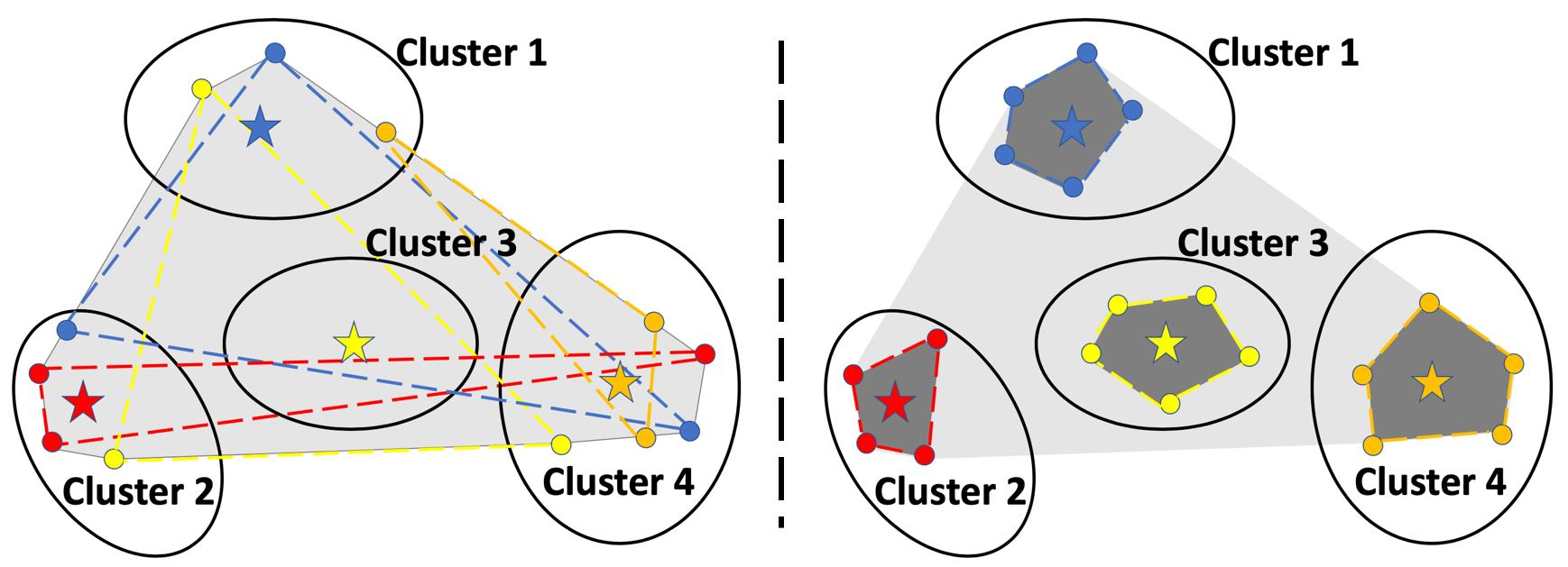
Figure 1: A multi-cluster dataset: Stars represent the learned bases, while circles denote representative samples for the basis of the same color. Left: The representative sets for the individual basis elements are unrestricted. Right: The representative sets are restricted to lie within their corresponding clusters.

Let ${\mathbf{X}}\in{}^{m\times n}$ denote a matrix of $n$ data samples of constant dimension $m$ arranged (summarized) column-wise, let ${\mathbf{D}}\in{}^{m\times k}$ denote the $k$ basis vectors used to represent the data and let $\bf{\Lambda}\in{}^{k\times n}$ stand for the low-dimension embedding matrix. The classical MF problem reads as:

$$\min_{{\mathbf{D}},\bf{\Lambda}}\lVert{\mathbf{X}}-{\mathbf{D}}{\bf{\Lambda}}\rVert^{2}+\lambda\lVert{\bf{\Lambda}}\rVert_{1}.$$ (1)

where $\lVert{\underline{x}}\rVert\triangleq\sqrt{{\underline{x}}^{T}{\underline{x}}}$ and $\lVert{\underline{x}}\rVert_{1}\triangleq{\sum_{j}\left\lvert{\underline{x}}[j]\right\rvert}$ denote the $\ell_{2}$-norm and $\ell_{1}$-norm of the vector ${\underline{x}}$, respectively.

In practice, ${\mathbf{X}}$ is inherently random and in the stochastic setting it is more adequate to minimize the above objective in expectation. In this case, the data approximation-error $g({\mathbf{D}})$ for a fixed ${\mathbf{D}}$ equals:

$$g({\mathbf{D}})\triangleq\operatorname{\mathbb{E}}_{\underline{\rm{X}}}[\min_{{\underline{\alpha}}\in{}^{k}}\lVert{\underline{\rm{X}}}-{\mathbf{D}}{\underline{\alpha}}\rVert^{2}+\lambda\lVert{\underline{\alpha}}\rVert_{1}],$$ (2)

where $\underline{\rm{X}}$ is a random vector of dimension $m$ and the parameter $\lambda$ controls the sparsity of the coefficient vector ${\underline{\alpha}}$. For analytical tractability, we assume that $\underline{\rm{X}}$ is drawn from the union of $k$ disjoint, convex compact regions (clusters), $\operatorname{{\mathcal{C}}}^{\lparen i\rparen}\in{}^{m},\,i\in[k]$. Each cluster is independently selected based on a given distribution, and the vector $\underline{\rm{X}}$ is sampled from the chosen cluster. Both the cluster and intra-cluster sample distributions are mildly constrained, as described in the next section.

The approximation-error of a single data sample ${\underline{x}}\in{}^{m}$ with respect to ${\mathbf{D}}$ equals

$$\ell({\underline{x}},{\mathbf{D}})\triangleq\min_{{\underline{\alpha}}\in{}^{k}}\frac{1}{2}\lVert{\underline{x}}-{\mathbf{D}}{\underline{\alpha}}\rVert^{2}+\lambda\lVert{\underline{\alpha}}\rVert_{1}.$$ (3)

Consequently, the approximation error-function $g({\mathbf{D}})$ in Equation 2 may be written as $g({\mathbf{D}})=\operatorname{\mathbb{E}}_{\underline{\rm{X}}}\left[\ell(\underline{\rm{X}},{\mathbf{D}})\right]$. The function $g({\mathbf{D}})$ is non-convex and optimizing it is NP-hard and requires prior knowledge of the distribution. To mitigate the latter problem, one can revert to an empirical estimate of $g({\mathbf{D}})$ involving the data samples ${\underline{x}}_{n}$, $n\in[t]$,

$$g_{t}({\mathbf{D}})=\frac{1}{t}\sum_{n=1}^{t}\ell({\underline{x}}_{n},{\mathbf{D}}).$$

Maintaining a running estimate of ${\mathbf{D}}_{t}$ of an optimizer of $g_{t}({\mathbf{D}})$ involves updating the coefficient vectors for all the data samples observed up to time $t$. Hence, it is desirable to use surrogate functions to simplify the updates. The surrogate function $\hat{g}_{t}({\mathbf{D}})$ proposed in Mairal et al. [2010] reads as

$$\hat{g}_{t}({\mathbf{D}})\triangleq\frac{1}{t}\sum_{n=1}^{t}{\frac{1}{2}\lVert{\underline{x}}_{n}-{\mathbf{D}}{\underline{\alpha}}_{n}\rVert^{2}+\lambda\lVert{\underline{\alpha}}_{n}\rVert_{1}},$$ (4)

where ${\underline{\alpha}}_{n}$ is an approximation of the optimal value of ${\underline{\alpha}}$ at step $n$, computed by solving Equation 3 with ${\mathbf{D}}$ fixed to ${\mathbf{D}}_{n-1}$, an optimizer of $\hat{g}_{n-1}({\mathbf{D}})$.

The above approach lends itself to an implementation of an online MF algorithm, as the sum in Equation 4 may be efficiently optimized whenever adding a new sample. However, in order to satisfy the convexity constraint of Ding et al. [2010], all previous values of ${\underline{x}}_{n}$ are needed to update ${\mathbf{D}}$. To mitigate this problem, we introduce for each cluster $\mathcal{C}^{(i)}$ a representative set $\hat{\mathbf{X}}^{({i})}_{t}\in{}^{m\times N_{i}}$ and its convex hull (representative region) $\operatorname{\operatorname{cvx}}\lparen\hat{\mathbf{X}}^{({i})}_{t}\rparen$. The values of $N_{i}$ are kept constant, and we require ${\mathbf{D}}_{t}[i]\in\operatorname{\operatorname{cvx}}\lparen\hat{\mathbf{X}}^{({i})}_{t}\rparen$. As illustrated in Figure 1, we may further restrict the representative regions as follows.

$\mathcal{R}_{u}$ (Figure 1, Left): We only require that $\hat{\mathbf{X}}^{({i})}_{t}\subset\operatorname{\operatorname{cvx}}\lparen\textstyle\bigcup_{j}\operatorname{{\mathcal{C}}}^{\lparen j\rparen}\rparen,i\in[k].$ This unrestricted case leads to an online solution for the cvxMF problem Ding et al. [2010] as one may use $\textstyle\bigcup_{j}\,\hat{\mathbf{X}}^{({j})}_{t}$ as a single representative region. The underlying online algorithms has provable performance guarantees.

$\mathcal{R}_{r}$ (Figure 1, Right): We require that $\hat{\mathbf{X}}^{({i})}_{t}\subset\operatorname{{\mathcal{C}}}^{\lparen i\rparen}$, which is a new cvxMF constraint for both the classical and online setting. Theoretical guarantees for the underlying algorithm follow from small and fairly-obvious modifications in the proof for the $\mathcal{R}_{u}$ case, assuming error-free sample classification.

3 Online Algorithm

The proposed online cvxMF method for solving $\mathcal{R}_{u}$ consists of two procedures, described in Algorithms 1 and 2. Algorithm 1 describes the initialization of the main procedure in Algorithm 2. Algorithm 1 generates an initial estimate for the basis ${\mathbf{D}}_{0}$ and for the representative regions $\{\operatorname{\operatorname{cvx}}\lparen\hat{\mathbf{X}}^{({i})}_{0}\rparen\}_{i\in[k]}$. A similar initialization was used in classical cvxMF, with the bases vectors obtained either through clustering (on a potentially subsampled dataset) or through random selection and additional processing [Ding et al., 2010]. During initialization, one first collects a fixed prescribed number of $N$ data samples, summarized in $\hat{\mathbf{X}}$. Subsequently, one runs the K-means algorithm on the collected samples to obtain a clustering, described by the cluster indicator matrix ${\mathbf{H}}\in\{0,1\}^{N\times k}$, in which ${\mathbf{H}}[n,i]=1$ if the $n$-th sample lies in cluster $i$. The sizes of the generated clusters $\left\{N_{i}\right\}_{i\in[k]}$ are used as fixed cardinalities of the representative sets of the online methods. The initial estimate of the basis ${\mathbf{D}}_{0}[i]$ equals the average of the samples inside the cluster, i.e. ${\mathbf{D}}_{0}\triangleq\hat{\mathbf{X}}\;{\mathbf{H}}\;{\operatorname{diag}(1/N_{1},\ldots,1/N_{k})}$.

Note again that initialization is performed using only a constant number of $N$ samples. Hence, K-means clustering does not significantly contribute to the complexity of the online algorithm. Second, to ensure that the restricted online cvxMF algorithm instantiates each cluster with at least one data sample, one needs to take into account the size of the smallest cluster (discussed in the Supplement).

Algorithm 1 Initialization

1:  Input: i.i.d samples ${\underline{x}}_{1},{\underline{x}}_{2},\dots,{\underline{x}}_{N}$ of a random vector $\underline{\rm{X}}\in{}^{m}$ summarized in $\hat{\mathbf{X}}$.

2:  Run K-means on $\hat{\mathbf{X}}$ to generate the cluster indicator matrix ${\mathbf{H}}\in\{0,1\}^{N\times k}$ and determine the initial cluster sizes (subsequent representative set sizes) $N_{i},i\in[k]$.

3:  Compute ${\mathbf{D}}_{0}$ and $\hat{\mathbf{X}}^{({i})}_{0}\in{}^{m\times N_{i}},~{}\forall i\in[k],$ according to:

$${\mathbf{D}}_{0}=\hat{\mathbf{X}}\;{\mathbf{H}}\;{\operatorname{diag}(1/N_{1},\ldots,1/N_{k})}$$

and summarize the initial representative sets of the clusters into matrices $\hat{\mathbf{X}}^{({i})}_{0},\,i=[k]$.

4:  Return: ${\mathbf{D}}_{0}$, $\{\hat{\mathbf{X}}^{({i})}_{0}\}_{i\in[k]}$.

Algorithm 2 Online cvxMF

1:  Input: Data samples ${\underline{x}}_{t}$, a parameter $\lambda\in\real$, and the maximum number of iterations $T$.

2:  Initialization: Compute ${\mathbf{D}}_{0}$, $\{\hat{\mathbf{X}}^{({i})}_{0}\}_{i\in[k]}$ using Algorithm 1. Set ${\mathbf{A}}_{0}=\bf 0$, ${\mathbf{B}}_{0}=\bf 0$.

3:  for $t=1$ to $T$ do

4:     Sample ${\underline{x}}_{t}$ from $\underline{\rm{X}}$.

5:     Update ${\underline{\alpha}}_{t}$ according to:

$${\underline{\alpha}}_{t}=\operatornamewithlimits{arg\,min}_{{\underline{\alpha}}\in{}^{k}}\frac{1}{2}\left\lVert{\underline{x}}_{t}-{\mathbf{D}}_{t-1}{\underline{\alpha}}\right\rVert^{2}+\lambda\lVert{\underline{\alpha}}\rVert_{1}.$$ (5)

6:     Set ${\mathbf{A}}_{t}=\frac{1}{t}\left\lparen\lparen t-1\rparen{\mathbf{A}}_{t-1}+{\underline{\alpha}}_{t}{\underline{\alpha}}_{t}^{T}\right\rparen$   and   ${\mathbf{B}}_{t}=\frac{1}{t}\left\lparen\lparen t-1\rparen{\mathbf{B}}_{t-1}+{\underline{x}}_{t}~{}{\underline{\alpha}}_{t}^{T}\right\rparen$.

7:     Choose the index of the basis $i_{t}$ to be updated according to $i_{t}={\rm{Uniform}}([k])$.

8:     Generate the augmented representative regions $\left\{\hat{\mathbf{Y}}^{\{l\}}_{{t}}\right\}_{l\in[N_{i_{t}}]\cup\{0\}}$:

$$\begin{gathered}\hat{\mathbf{Y}}^{\{0\}}_{{t}}=\hat{\mathbf{X}}^{({i_{t}})}_{t-1}\\ \left\{\hat{\mathbf{Y}}^{\{l\}}_{{t}}\right\}_{l\in[N_{i_{t}}]}:~{}\hat{\mathbf{Y}}^{\{l\}}_{{t}}[j]=\begin{cases}\hat{\mathbf{X}}^{({i_{t}})}_{t-1}[j],&\text{ if }j\in[N_{i}]\setminus l\\ {\underline{x}}_{t},&\text{ if }j=l.\\ \end{cases}\end{gathered}$$ (6)

9:     Update $\{\hat{\mathbf{X}}^{({i})}_{t}\}_{i\in[k]}$ and ${\mathbf{D}}_{t}$ by executing the following two steps:

1. Compute $l^{\star},\hat{\mathbf{D}}^{\star}$ by solving the optimization problems:

   $$l^{\star},\hat{\mathbf{D}}^{\star} =\operatornamewithlimits{arg\,min}_{\begin{subarray}{c}l,~{}{\mathbf{D}}\;\text{ s.t. }\\ {\mathbf{D}}[j]\in\operatorname{\operatorname{cvx}}\left\lparen\hat{\mathbf{X}}^{({j})}_{t-1}\right\rparen~{}j\neq i_{t},\\ {\mathbf{D}}[i_{t}]\in\operatorname{\operatorname{cvx}}\left\lparen\hat{\mathbf{Y}}^{\{l\}}_{{t}}\right\rparen\end{subarray}}\frac{1}{t}\sum_{n=1}^{t}\left\lparen\frac{1}{2}\left\lVert{\underline{x}}_{n}-{\mathbf{D}}{\underline{\alpha}}_{n}\right\rVert^{2}+\lambda\lVert{\underline{\alpha}}_{n}\rVert_{1}\right\rparen,$$

   $$\begin{split}&=\displaystyle\operatornamewithlimits{arg\,min}_{\begin{subarray}{c}l,~{}{\mathbf{D}}\;\text{ s.t. }\\ {\mathbf{D}}[j]\in\operatorname{\operatorname{cvx}}\left\lparen\hat{\mathbf{X}}^{({j})}_{t-1}\right\rparen~{}j\neq i_{t},\\ {\mathbf{D}}[i_{t}]\in\operatorname{\operatorname{cvx}}\left\lparen\hat{\mathbf{Y}}^{\{l\}}_{{t}}\right\rparen\end{subarray}}\frac{1}{2}\operatorname{Tr}({\mathbf{D}}^{T}{\mathbf{D}}{\mathbf{A}}_{t})-\operatorname{Tr}({\mathbf{D}}^{T}{\mathbf{B}}_{t}).\end{split}$$ (7)

2. Set

   $$\hat{\mathbf{X}}^{({i})}_{t} =\begin{cases}\hat{\mathbf{Y}}^{\{l^{\star}\}}_{{t}},&\text{ if }i=i_{t}\\ \hat{\mathbf{X}}^{({i})}_{t-1},&\text{ if }i\in[k]\setminus i_{t},\end{cases}$$

   $${\mathbf{D}}_{t} =\hat{\mathbf{D}}^{\star}.$$

10:  end for

11:  return  ${\mathbf{D}}_{T}$, the learned convex dictionary.

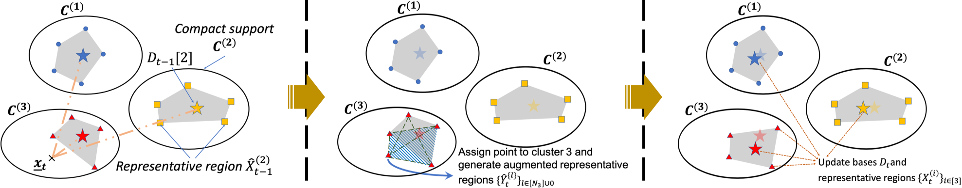
Figure 2: Illustration of one step of the online cvxMF algorithm with multiple-representative regions.

Following initialization, Algorithm 2 sequentially selects one sample ${\underline{x}}_{t}$ at a time and then updates the current representative sets $\hat{\mathbf{X}}^{({i})}_{t},i\in[k],$ and bases ${\mathbf{D}}_{t}$. More precisely, after computing the coefficient vector ${\underline{\alpha}}_{t}$ in Step 5, one places the sample ${\underline{x}}_{t}$ into the appropriate cluster, indexed by $i_{t}$. The $N_{i_{t}}$-subsets of $\{\operatorname{col}(\hat{\mathbf{X}}^{({i_{t}})}_{t})\cup{\underline{x}}_{t}\}$ (referred to as the augmented representative sets $\hat{\mathbf{Y}}^{\{l\}}_{{t}}$, $l\in[N_{i_{t}}]\cup\{0\}$), are used in Steps 8 and 9 to determine the new representative region $\hat{\mathbf{X}}^{({i_{t}})}_{t+1}$ for cluster $i_{t}$. To find the optimal index $l\in[N_{i_{t}}]\cup\{0\}$ and the corresponding updated basis ${\mathbf{D}}[i_{t}]$, in Step 9 we solve $N_{i_{t}}$ convex problems. The minimum of the optimal solutions of these optimization problems determines the new bases ${\mathbf{D}}_{t}$ and the representative regions $\hat{\mathbf{X}}^{({i})}_{t}$ (see Figure 2 for clarifications). Note that the combinatorial search step is executed on a constant-sized set of samples and is hence computationally efficient.

In Step $7$, the new sample may be assigned to a cluster in two different ways. For the case $\mathcal{R}_{u}$, we use a random assignment. For the case $\mathcal{R}_{r}$, we need to perform the correct sample assignment in order to establish theoretical guarantees for the algorithm. Extensive simulations show that using $i_{t}=\operatornamewithlimits{arg\,max}{\underline{\alpha}}_{t}$ works very well in practice. Note that in either case, in order to minimize $g({\mathbf{D}}),$ one does not necessarily require an error-free classification process.

4 Convergence Analysis

In what follows, we show that the sequence of dictionaries $\{{\mathbf{D}}_{t}\}_{t}$ converges almost surely to a stationary point of $g({\mathbf{D}})$ under assumptions similar to those used in Mairal et al. [2010], listed below.

1. The data distribution on a compact support set ${\mathcal{C}}$ has bounded “skewness”. The compact support assumption naturally arises in many practical applications. The bounded skewness assumption for the distribution of $\underline{\rm{X}}$ reads as

   $$\operatorname{\mathbb{P}}\lparen\lVert{\underline{\rm{X}}}-{\underline{p}}\rVert\leq r~{}|~{}\underline{\rm{X}}\in\operatorname{{\mathcal{C}}}\rparen\geq\kappa\,{\operatorname{vol}\left\lparen B(r,{\underline{p}})\right\rparen}/{\operatorname{vol}\left\lparen\operatorname{{\mathcal{C}}}\right\rparen},$$ (8)

   where $\operatorname{{\mathcal{C}}}\triangleq\operatorname{\operatorname{cvx}}\lparen\textstyle\bigcup_{i}\operatorname{{\mathcal{C}}}^{\lparen i\rparen}\rparen$, $\kappa$ is a positive constant and $B(r,{\underline{p}})=\{{{\underline{x}}:\,\lVert{\underline{x}}-{\underline{p}}\rVert\leq r\}}$ stands for the ball of radius $r$ around ${\underline{p}}\in\operatorname{{\mathcal{C}}}$. This assumption is satisfied for appropriate values of $\kappa$ and distributions of $\underline{\rm{X}}$ that are “close” to uniform.

2. The quadratic surrogate functions $\hat{g}_{t}$ are strictly convex, and have Hessians that are lower-bounded by a positive constant $\kappa_{1}>0$. It is straightforward to enforce this assumption by adding a term $\frac{\kappa_{1}}{2}||{\mathbf{D}}||_{F}^{2}$ to the surrogate or original objective function; this leads to replacing the positive semi-definite matrix $\frac{1}{t}{\mathbf{A}}_{t}$ in LABEL:eq:dic_update by $\frac{1}{t}{\mathbf{A}}_{t}+\kappa_{1}I$.

3. The approximation-error function $\ell({\underline{x}},{\mathbf{D}})$ is “well-behaved”. We assume that the function $\ell({\underline{x}},{\mathbf{D}})$ defined in Equation 3 is continuously differentiable, and that its expectation $g({\mathbf{D}})=\operatorname{\mathbb{E}}_{\underline{\rm{X}}}[\ell(\underline{\rm{X}},{\mathbf{D}})]$ is continuously differentiable and Lipschitz on the compact set $\operatorname{{\mathcal{C}}}$. This assumption parallels the one made in [Mairal et al., 2010, Proposition 2], and it holds if the solution to Equation 3 is unique. The uniqueness condition can be enforced by adding a regularization term $\kappa\lVert{\underline{\alpha}}\rVert_{2}^{2}$ ($\kappa>0$) to $\ell(\cdot)$ in Equation 3. This term makes the (LARS) optimization problem in Equation 5 strictly convex and hence ensures that it has a unique solution.

In addition, recall the definition of ${\mathbf{D}}_{t}$ and define ${\mathbf{D}}^{\star}_{t}$ as the global optima of the surrogate $\hat{g}_{t}({\mathbf{D}}),$

$${\mathbf{D}}_{t} =\operatornamewithlimits{arg\,min}_{{\mathbf{D}}[i]\in\operatorname{\operatorname{cvx}}\lparen\hat{\mathbf{X}}^{({i})}_{t}\rparen,\;i\in[k]}\hat{g}_{t}({\mathbf{D}})$$

$${\mathbf{D}}^{\star}_{t} =\operatornamewithlimits{arg\,min}_{{\mathbf{D}}[i]\in\operatorname{{\mathcal{C}}},~{}i\in[k]}\hat{g}_{t}({\mathbf{D}}).$$

4.1 Main Results

Theorem 1.

Under assumptions (A.1), (A.2) and (A.3), the sequence $\{{\mathbf{D}}_{t}\}_{t}$ converges almost surely to a stationary point of $g({\mathbf{D}})$.

Lemma 2 bounds the difference of the surrogates for two different dictionary arguments. Lemma 3 establishes that restricting the optima of the surrogate function $\hat{g}_{t}({\mathbf{D}})$ to the representative region $\operatorname{\operatorname{cvx}}\lparen\hat{\mathbf{X}}^{({i})}_{t}\rparen$ does not affect convergence to the asymptotic global optima ${\mathbf{D}}^{\star}_{\infty}$. Lemma 4 establishes that Algorithm 2 converges almost surely and that the limit is an optima ${\mathbf{D}}^{\star}_{\infty}$. Based on the results in Lemma 4, Theorem 1 establishes that the generated sequence of dictionaries ${\mathbf{D}}_{t}$ converges to a stationary point of $g({\mathbf{D}})$. The proofs are relegated to the Supplement, but sketched below.

Let $\Delta_{t}\triangleq\lvert\hat{g}_{t}({\mathbf{D}}_{t})-\hat{g}_{t}({\mathbf{D}}^{\star}_{t})\rvert$ denote the difference between the surrogate functions for an unrestricted basis and a basis for which one requires ${\mathbf{D}}_{t}[i]\in\operatorname{\operatorname{cvx}}\left\lparen\hat{\mathbf{X}}^{({i})}_{t}\right\rparen$. Then, one can show that

$$\Delta_{t}\leq\min\left\{\Delta_{t-1},\left\lvert\hat{g}_{t-1}({\mathbf{D}}_{t})-\hat{g}_{t-1}({\mathbf{D}}^{\star}_{t-1})\right\rvert\right\}+O\left\lparen\frac{1}{t}\right\rparen.$$

Based on an upper bound on the error of random coordinate descent used for minimizing the surrogate function and assumption (A.1), one can derive a recurrence relation for $\operatorname{\mathbb{E}}[\Delta_{t}]$, described in the lemma below. This recurrence establishes a rate of decrease of $O\left\lparen\frac{1}{t^{2/(m+2)}}\right\rparen$ for $\operatorname{\mathbb{E}}[\Delta_{t}]$.

Lemma 2.

Let $\Delta_{t}\triangleq\hat{g}_{t}({\mathbf{D}}_{t})-\hat{g}_{t}({\mathbf{D}}^{\star}_{t})$. Then

$$\operatorname{\mathbb{E}}\left[\Delta_{t}\right]\leq O\left\lparen\frac{1}{t}\right\rparen+\operatorname{\mathbb{E}}\left[\Delta_{t-1}\right]-V_{m}~{}\operatorname{\mathbb{E}}\left[\Delta_{t-1}\right]^{\frac{m+2}{2}},$$

where $V_{m}\triangleq\frac{8\kappa\min_{i}p_{i}~{}\frac{\pi^{\frac{m}{2}}}{\Gamma\lparen\frac{m}{2}+1\rparen}}{c_{\hat{g}}(m+2)\operatorname{vol}\left\lparen\operatorname{{\mathcal{C}}}\right\rparen}\left\lparen\frac{2}{A~{}k}\right\rparen^{m/2},$ and $\kappa$ is the same constant used in Equation 8 of assumption (A.1). Also, $A=\max_{i}{\mathbf{A}}_{t}[i,i]$, $\forall\;t$, while $c_{\hat{g}}$ denotes a bound on the condition number of ${\mathbf{A}}_{t},~{}\forall t,$ and $p_{i}$ denotes the probability of choosing $i_{t}=i$ in Step 7 of Algorithm 2.

Lemma 3 establishes that the optima ${\mathbf{D}}_{t}$ confined to the representative region and the global optima ${\mathbf{D}}^{\star}_{t}$ are close. From the Lipschitz continuity of $\hat{g}_{t}({\mathbf{D}})$ asserted in assumptions (A.1) and (A.2), we can show that $\Delta_{t}=\lVert{\mathbf{D}}_{t}-{\mathbf{D}}^{\star}_{t}\rVert_{\hat{g}_{t}}\leq\lVert{\mathbf{D}}_{t}-{\mathbf{D}}^{\star}_{t}\rVert$. Lemma 3 then follows from Lemma 2 by applying the quasi-martingale convergence theorem stated in the Supplement.

Lemma 3.

$\sum_{t}\frac{\lVert{\mathbf{D}}_{t}-{\mathbf{D}}^{\star}_{t}\rVert}{t+1}$ converges almost surely.

Lemma 4.

The following claims hold true:

1. $\hat{g}_{t}({\mathbf{D}}_{t})$ and $\hat{g}_{t}({\mathbf{D}}^{\star}_{t})$ converge almost surely;

2. $\hat{g}_{t}({\mathbf{D}}_{t})-\hat{g}_{t}({\mathbf{D}}^{\star}_{t})$ converges almost surely to $0$;

3. $\hat{g}_{t}({\mathbf{D}}^{\star}_{t})-g({\mathbf{D}}^{\star}_{t})$ converges almost surely to $0$;

4. $g({\mathbf{D}}^{\star}_{t})$ converges almost surely .

The proofs of P1) and P2) involve completely new analytic approaches described in the Supplement.

5 Experimental Validation

We compare the approximation error and running time of our proposed online cvxMF algorithm with non-negative MF (NMF), cvxMF [Ding et al., 2010] and online MF [Mairal et al., 2010]. For datasets with a ground truth, we also report the clustering accuracy. The datasets used include a) clusters of synthetic data samples; b) MNIST handwritten digits [LeCun et al., 1998]; c) single-cell RNA sequencing datasets Zheng et al. [2017] and d) four other real world datasets from the UCI Machine Learning repository [Dua and Graff, 2017]. The largest sample size scales as $10^{6}$.

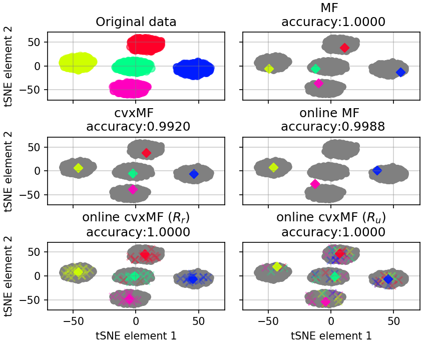
(a)

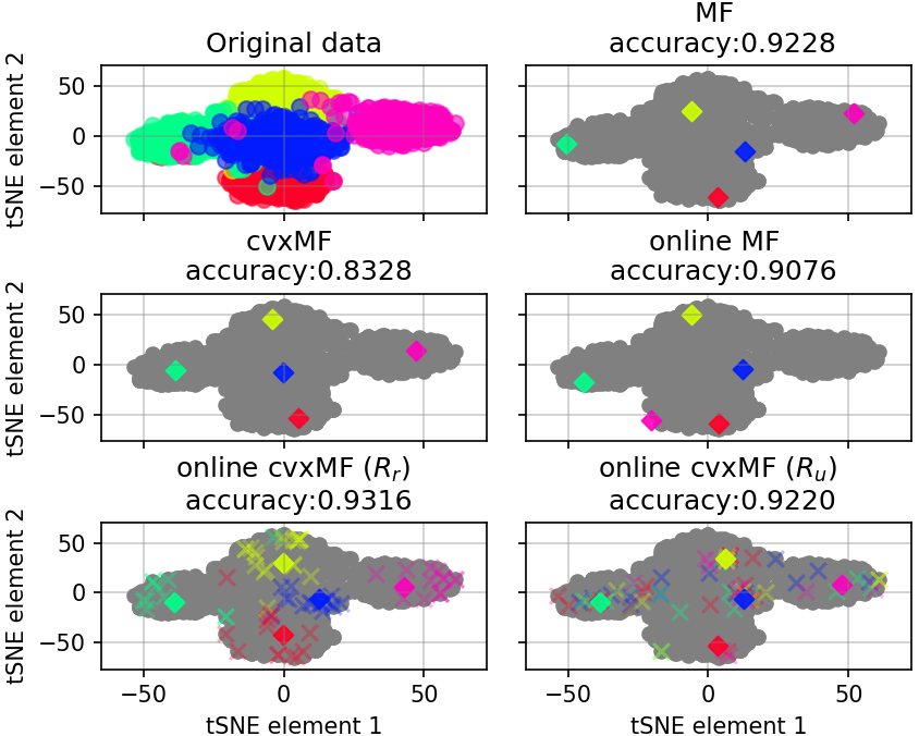
(b)

Figure 3: Results for Gaussian mixtures with color-coded clusters. Here, tSNE stands for the t-distributed stochastic neighbor embedding [Maaten and Hinton, 2008], in which the $x$-axis represents the first and the $y$-axis the second element of the embedding. Color-coded circles represent samples, diamonds represent basis vectors learned by the different algorithms, while crosses describe samples in the representative regions. The “interpretability property” can be easily observed visually.

Synthetic Datasets. The synthetic datasets were generated by sampling from a $3\sigma$-truncated Gaussian mixture model with $5$ components, and with samples-sizes in $[10^{3},10^{6}]$. Each component Gaussian has an expected value drawn uniformly at random from $[0,20]$ while the mixture covariance matrix equals the identity matrix $I$ (“well-separated clusters”) or $2.5\,I$ ("overlapping clusters"). We ran the online cvxMF algorithm with both unconstrained $\mathcal{R}_{u}$ and restricted $\mathcal{R}_{r}$ representative regions, and used the normalization factor $\lambda={c}/{\sqrt{m}}$ suggested in Bickel et al. [2009]. After performing cross validation on an evaluation set of size $1000$, we selected $c=0.2$. Figure 3 shows the results for two synthetic datasets each of size $n=2,500$ and with $N=150$. The sample size was restricted for ease of visualization and to accommodate the cvxMF method which cannot run on larger sets. The number of iterations was limited to $1,200$. Both the cvxMF and online cvxMF algorithms generate bases that provide excellent representations of the data clusters. The MF and online MF method produce bases that are hard to interpret and fail to cover all clusters. Note that for the unrestricted version of cvxMF, samples of one representative set may belong to multiple clusters.

For the same Gaussian mixture model but larger datasets, we present running times and times to convergence (or, if convergence is slow, the maximum number of iterations) in Figure 4 (a) and (b), respectively. For well-separated synthetic datasets, we let $n$ increase from $10^{2}$ to $10^{6}$ and plot the results in (a). The non-online cvxMF algorithm becomes intractable after $10^{4}$ sample, while the cvxMF and MF easily scale for $10^{6}$ and more samples. To illustrate the convergence, we used a synthetic dataset with $n=5,000$ in order to ensure that all four algorithms converge within $100$s. Figure 4 (b) plots the approximation error $l_{2}=\frac{1}{n}\lVert{\mathbf{X}}-{\mathbf{D}}{\bf\Lambda}\rVert$ with respect to the running time. We chose a small value of $n$ so as to be able to run all algorithms, and for this case the online algorithms may have larger errors. But as already pointed out, as $n$ increases, non-online algorithms become intractable while the online counterparts operate efficiently (and with provable guarantees).

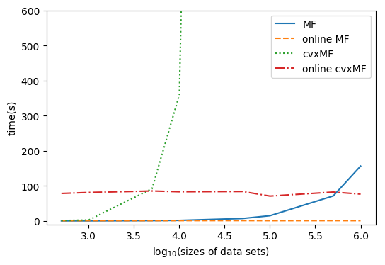
(a)

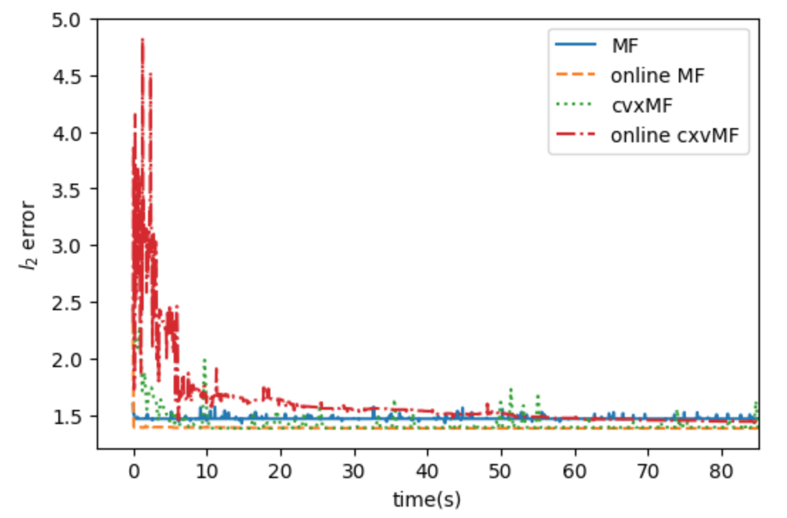
(b)

Figure 4: (a): Running times (s) vs. the log of the dataset sizes; (b) Running times (s) vs. the $l_{2}$ error.

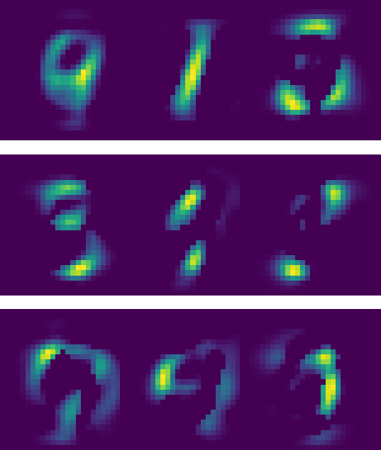
(a)

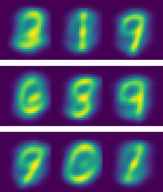
(b)

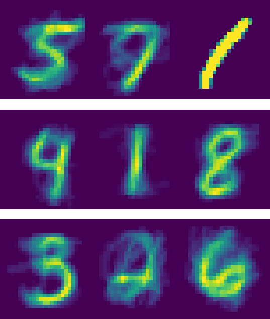
(c)

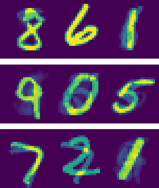
(d)

Figure 5: MNIST results (as the eigenimage set is overcomplete, clustering accuracy is omitted).

The MNIST Dataset. The MNIST dataset was subsampled to a smaller set of $10,000$ images of resolution $28\times 28$ to illustrate the performance of both the cvxMF and online cvxMF methods on image datasets. All algorithms ran $3,000$ iterations with $N=150$ and $\lambda=0.1$ to generate “eigenimages,” capturing the characteristic features used as bases [Leonardis and Bischof, 2000]. Figure 5 plots the first $9$ eigenimages. The results for the ${\mathcal{R}}_{u}$ algorithm are similar to that of the non-online cvxMF algorithm and omitted. CvxMF produces blurry images since one averages all samples. The results are significantly better for the ${\mathcal{R}}_{r}$ case, as one only averages a small subset of representative samples.

Single-Cell (sc) RNA Data. scRNA datatsets contain expressions (activities) of all genes in individual cells, and each cell represents one data sample. Cells from the same tissue under same cellular condition tend to cluster, and due to the fact that that the sampled tissue are known, the cell labels are known a priori. This setting allows us to investigate the ${\mathcal{R}}_{r}$ version of the online cvxMF algorithm to identify “typical” samples. For our dataset, described in more detail in the Supplement, the two non-online method failed to converge and required significantly larger memory. Hence, we only present results for the online methods.

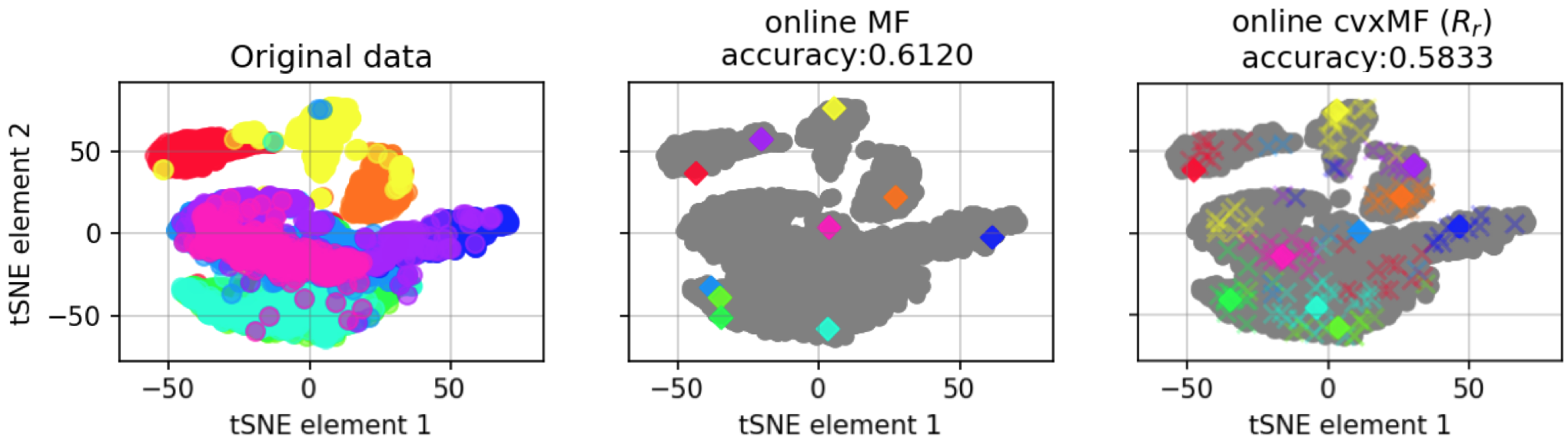
Figure 6: Results for the online methods executed on a blood-cell scRNA dataset.

Results pertaining to real world datasets from the UCI Machine Learning repository Dua and Graff [2017], also used for testing cvxMF Ding et al. [2010], are presented in the Supplement.

6 Acknowledgement

The authors are grateful to Prof. Bruce Hajek for valuable discussions. This work was funded by the DB2K NIH 3U01CA198943-02S1, NSF/IUCR CCBGM Center, and the SVCF CZI 2018-182799 2018-182797.

References

- Bach et al. [2008] Francis Bach, Julien Mairal, and Jean Ponce. Convex sparse matrix factorizations. arXiv preprint arXiv:0812.1869, 2008.
- Bickel et al. [2009] Peter J Bickel, Ya’acov Ritov, Alexandre B Tsybakov, et al. Simultaneous analysis of lasso and dantzig selector. The Annals of Statistics, 37(4):1705–1732, 2009.
- Blum et al. [2016] Avrim Blum, Sariel Har-Peled, and Benjamin Raichel. Sparse approximation via generating point sets. In Proceedings of the twenty-seventh annual ACM-SIAM symposium on Discrete algorithms, pages 548–557. Society for Industrial and Applied Mathematics, 2016.
- Bouchard et al. [2013] Guillaume Bouchard, Dawei Yin, and Shengbo Guo. Convex collective matrix factorization. In Artificial Intelligence and Statistics, pages 144–152, 2013.
- Dai et al. [2012] Wei Dai, Tao Xu, and Wenwu Wang. Simultaneous codeword optimization (simco) for dictionary update and learning. IEEE Transactions on Signal Processing, 60(12):6340–6353, 2012.
- Ding et al. [2010] Chris HQ Ding, Tao Li, and Michael I Jordan. Convex and semi-nonnegative matrix factorizations. IEEE transactions on pattern analysis and machine intelligence, 32(1):45–55, 2010.
- Dua and Graff [2017] Dheeru Dua and Casey Graff. UCI machine learning repository, 2017. URL http://archive.ics.uci.edu/ml.
- Esser et al. [2012] Ernie Esser, Michael Moller, Stanley Osher, Guillermo Sapiro, and Jack Xin. A convex model for nonnegative matrix factorization and dimensionality reduction on physical space. IEEE Transactions on Image Processing, 21(7):3239–3252, 2012.
- Févotte and Dobigeon [2015] Cédric Févotte and Nicolas Dobigeon. Nonlinear hyperspectral unmixing with robust nonnegative matrix factorization. IEEE Transactions on Image Processing, 24(12):4810–4819, 2015.
- Gillis and Glineur [2012] Nicolas Gillis and François Glineur. Accelerated multiplicative updates and hierarchical als algorithms for nonnegative matrix factorization. Neural computation, 24(4):1085–1105, 2012.
- Gribonval et al. [2015] Rémi Gribonval, Rodolphe Jenatton, Francis Bach, Martin Kleinsteuber, and Matthias Seibert. Sample complexity of dictionary learning and other matrix factorizations. IEEE Transactions on Information Theory, 61(6):3469–3486, 2015.
- Kasiviswanathan et al. [2012] Shiva P Kasiviswanathan, Huahua Wang, Arindam Banerjee, and Prem Melville. Online l1-dictionary learning with application to novel document detection. In Advances in Neural Information Processing Systems, pages 2258–2266, 2012.
- LeCun et al. [1998] Yann LeCun, Léon Bottou, Yoshua Bengio, Patrick Haffner, et al. Gradient-based learning applied to document recognition. Proceedings of the IEEE, 86(11):2278–2324, 1998.
- Lee and Seung [2001] Daniel D Lee and H Sebastian Seung. Algorithms for non-negative matrix factorization. In Advances in neural information processing systems, pages 556–562, 2001.
- Lee et al. [2007] Honglak Lee, Alexis Battle, Rajat Raina, and Andrew Y Ng. Efficient sparse coding algorithms. In Advances in neural information processing systems, pages 801–808, 2007.
- Leonardis and Bischof [2000] Aleš Leonardis and Horst Bischof. Robust recognition using eigenimages. Computer Vision and Image Understanding, 78(1):99–118, 2000.
- Li et al. [2016] Xingguo Li, Zhaoran Wang, Junwei Lu, Raman Arora, Jarvis Haupt, Han Liu, and Tuo Zhao. Symmetry, saddle points, and global geometry of nonconvex matrix factorization. arXiv preprint arXiv:1612.09296, 2016.
- Lin [2007] Chih-Jen Lin. Projected gradient methods for nonnegative matrix factorization. Neural computation, 19(10):2756–2779, 2007.
- Liu et al. [2012] Haifeng Liu, Zhaohui Wu, Xuelong Li, Deng Cai, and Thomas S Huang. Constrained nonnegative matrix factorization for image representation. IEEE Transactions on Pattern Analysis and Machine Intelligence, 34(7):1299–1311, 2012.
- Maaten and Hinton [2008] Laurens van der Maaten and Geoffrey Hinton. Visualizing data using t-sne. Journal of machine learning research, 9(Nov):2579–2605, 2008.
- Mairal et al. [2009] Julien Mairal, Jean Ponce, Guillermo Sapiro, Andrew Zisserman, and Francis R Bach. Supervised dictionary learning. In Advances in neural information processing systems, pages 1033–1040, 2009.
- Mairal et al. [2010] Julien Mairal, Francis Bach, Jean Ponce, and Guillermo Sapiro. Online learning for matrix factorization and sparse coding. Journal of Machine Learning Research, 11(Jan):19–60, 2010.
- Mei et al. [2018] Jieru Mei, Chunyu Wang, and Wenjun Zeng. Online dictionary learning for approximate archetypal analysis. In Proceedings of the European Conference on Computer Vision (ECCV), pages 486–501, 2018.
- Paatero and Tapper [1994] Pentti Paatero and Unto Tapper. Positive matrix factorization: A non-negative factor model with optimal utilization of error estimates of data values. Environmetrics, 5(2):111–126, 1994.
- Rubinstein et al. [2010] Ron Rubinstein, Michael Zibulevsky, and Michael Elad. Double sparsity: Learning sparse dictionaries for sparse signal approximation. IEEE Transactions on signal processing, 58(3):1553–1564, 2010.
- Srebro et al. [2005] Nathan Srebro, Jason Rennie, and Tommi S Jaakkola. Maximum-margin matrix factorization. In Advances in neural information processing systems, pages 1329–1336, 2005.
- Tang et al. [2016] Jun Tang, Ke Wang, and Ling Shao. Supervised matrix factorization hashing for cross-modal retrieval. IEEE Transactions on Image Processing, 25(7):3157–3166, 2016.
- Tosic and Frossard [2011] Ivana Tosic and Pascal Frossard. Dictionary learning. IEEE Signal Processing Magazine, 28(2):27–38, 2011.
- Van Der Maaten et al. [2009] Laurens Van Der Maaten, Eric Postma, and Jaap Van den Herik. Dimensionality reduction: a comparative. J Mach Learn Res, 10:66–71, 2009.
- Vavasis [2009] Stephen A Vavasis. On the complexity of nonnegative matrix factorization. SIAM Journal on Optimization, 20(3):1364–1377, 2009.
- Wang et al. [2017] Xiao Wang, Peng Cui, Jing Wang, Jian Pei, Wenwu Zhu, and Shiqiang Yang. Community preserving network embedding. In Thirty-First AAAI Conference on Artificial Intelligence, 2017.
- Xia et al. [2019] Rui Xia, Vincent YF Tan, Louis Filstroff, and Cédric Févotte. A ranking model motivated by nonnegative matrix factorization with applications to tennis tournaments. arXiv preprint arXiv:1903.06500, 2019.
- Zhao and Tan [2016] Renbo Zhao and Vincent YF Tan. Online nonnegative matrix factorization with outliers. In 2016 IEEE International Conference on Acoustics, Speech and Signal Processing (ICASSP), pages 2662–2666. IEEE, 2016.
- Zhao et al. [2016] Renbo Zhao, Vincent YF Tan, and Huan Xu. Online nonnegative matrix factorization with general divergences. arXiv preprint arXiv:1608.00075, 2016.
- Zheng et al. [2017] Grace XY Zheng, Jessica M Terry, Phillip Belgrader, Paul Ryvkin, Zachary W Bent, Ryan Wilson, Solongo B Ziraldo, Tobias D Wheeler, Geoff P McDermott, Junjie Zhu, et al. Massively parallel digital transcriptional profiling of single cells. Nature communications, 8:14049, 2017.