TU–1085

UV contributions to energy of a static quark-antiquark pair
in large-$\beta_{0}$ approximation

Yuuki Hayashi and Yukinari Sumino
Department of Physics, Tohoku University
Sendai, 980-8578 Japan

The total energy of a static quark-antiquark pair $E_{\rm tot}(r)=2m_{\rm pole}+V_{\rm QCD}(r)$ is known to include ${\cal O}(\Lambda_{\rm QCD}^{3}r^{2})$ and ${\cal O}(\Lambda_{\rm QCD}^{3}/\overline{m}^{2})$ renormalon uncertainties in the large-$\beta_{0}$ approximation, after canceling ${\cal O}(\Lambda_{\rm QCD})$ renormalons. We compute the (renormalon-free) genuine UV part in terms of the $\overline{\rm MS}$ mass $\overline{m}$, extending a recently-proposed method which conforms with OPE. In particular the $r$-independent part is determined. The result would help understanding the nature of $E_{\rm tot}(r)$ in the context of OPE with renormalon subtraction.

Being much smaller than ordinary hadrons, a hadron composed of a heavy quark and its anti-particle (heavy quarkonium) is an ideal system that can be systematically analyzed using solid analysis tools of the strong interaction, such as perturbative QCD and operator product expansion (OPE). In particular various analyses of the leading-order total energy of this system, defined by $E_{\rm tot}(r)\equiv 2m_{\rm pole}+V_{\rm QCD}(r)$, have provided a lot of insight into the theoretical structure of perturbative QCD and OPE. The analyses were brought to a new phase by the discovery of the cancellation of ${\cal O}(\Lambda_{\rm QCD})$ renormalons in $E_{\rm tot}(r)$ [1, 2, 3], which led to a dramatic improvement in convergence of perturbative series of $E_{\rm tot}(r)$ and to much more accurate computation.

Series of studies [4, 5, 6, 7, 8] on the static QCD potential $V_{\rm QCD}(r)$ in perturbative QCD have shown that the potential can be expressed in an expansion in $r$ in the form

$$V_{\rm QCD}(r)=V_{C}(r)+C_{0}^{V}+C_{1}^{V}r+{\cal O}(\Lambda_{\rm QCD}^{3}r^{2})~{}~{}~{}\mbox{for}~{}~{}r\ll\Lambda_{\rm QCD}^{-1}\,,$$ (1)

by resumming logarithms by renormalization group (RG) or in the large-$\beta_{0}$ approximation. Here, the $r$-independent constant $C_{0}^{V}$ includes ${\cal O}(\Lambda_{\rm QCD})$ renormalon; $V_{C}(r)$ and $C_{1}^{V}r$ correspond to genuinely ultraviolet (UV) part and can be computed without renormalon uncertainties. $V_{C}(r)$ has a Coulomb-like form with logarithmic corrections at short-distances. The above expansion in $r$ is consistent with OPE performed in an effective field theory (EFT) “potential non-relativistic QCD” (pNRQCD) [9]. In fact, $V_{C}(r)+C_{1}^{V}r$ can be identified with the leading Wilson coefficient of OPE of $V_{\rm QCD}(r)$ after subtraction of renormalons. This OPE of $V_{\rm QCD}(r)$ is formulated beyond the large-$\beta_{0}$ approximation (i.e., including sub-leading logarithms), and recently it has been applied to a precise determination of $\alpha_{s}(M_{Z})$ by comparing the above prediction with lattice computation in an OPE framework, in which the ${\cal O}(\Lambda_{\rm QCD})$ and ${\cal O}(\Lambda_{\rm QCD}^{3}r^{2})$ renormalons are subtracted [10, 11].

Refs. [7, 8] have developed a prescription [referred to as “Contour Deformation (CD) prescription” hereafter], which performs an expansion of a general observable $X(Q)$ in the inverse of the hard scale $Q$, after resummation to all orders in $\alpha_{s}$ within the large-$\beta_{0}$ approximation. ($1/Q=r$ in the case of the QCD potential.) This prescription achieves separation of UV and infrared (IR) contributions in a natural way. Furthermore, a detailed connection of this expansion to OPE is given through the expansion-by-region technique.

Similarly to the QCD potential, we expect that, when expressed in terms of a short-distance mass $\overline{m}$, the pole mass of a heavy quark can be expressed in the form

$$m_{\rm pole}=\overline{m}+\Delta M_{0}(\overline{m})+C_{0}^{m}+\frac{C_{1}^{m}}{\overline{m}}+{\cal O}(\Lambda_{\rm QCD}^{3}/\overline{m}^{2})~{}~{}~{}\mbox{for}~{}~{}\overline{m}\gg\Lambda_{\rm QCD}\,,$$ (2)

where the $\overline{m}$-independent constant $C_{0}^{m}$ includes ${\cal O}(\Lambda_{\rm QCD})$ renormalon; $\Delta M_{0}(\overline{m})$ denotes the part proportional to $\overline{m}$ with logarithmic corrections at large $\overline{m}$. Nevertheless, even in the case restricting to the large-$\beta_{0}$ approximation, there is a difficulty to apply the CD prescription to carry out this expansion. The difficulty comes from (UV) renormalization of the pole mass, and we need to devise an extension of the prescription to deal with it.

As already mentioned, in the combination $2C_{0}^{m}+C_{0}^{V}$, the ${\cal O}(\Lambda_{\rm QCD})$ renormalons cancel. As a result $E_{\rm tot}(r)$ can be computed up to ${\cal O}(\Lambda_{\rm QCD}^{3}r^{2})$ and ${\cal O}(\Lambda_{\rm QCD}^{3}/\overline{m}^{2})$ renormalon uncertainties. The explicit expression of this computable part of $E_{\rm tot}(r)$ should depend on the definition of the short-distance mass $\overline{m}$ to be used. Analytic or semi-analytic analyses of this computable part have been missing. The purpose of this paper is to give an explicit expression for it and to provide a semi-analytic analysis, in the case we choose the $\overline{\rm MS}$ mass for $\overline{m}$ and within the large-$\beta_{0}$ approximation. An interesting question may be as follows: Is there a constant term proportional to $\Lambda_{\rm QCD}$ (independent of $r$ and $\overline{m}$) included in this computable part? [Noting that $C_{1}^{V}r=(2\pi e^{5/3}C_{F}/\beta_{0})\Lambda_{\rm QCD}^{2}r$ in the large-$\beta_{0}$ approximation, this may not be a completely absurd question. For instance, one may suspect a possibility that different short-distance masses are mutually related by an ${\cal O}(\Lambda_{\rm QCD})$ difference.]

Subtraction of the ${\cal O}(\Lambda_{\rm QCD})$ renormalons from $E_{\rm tot}(r)$ and $m_{\rm pole}$ has also been studied in [14, 15] in connection with pNRQCD EFT. The analyses concern how to subtract the renormalons from finite-order perturbative series (not restricting to the large-$\beta_{0}$ approximation). A major difference of our method is that (in the large-$\beta_{0}$ approximation) we resum the series to all orders and extract a renormalon-free part in the form which conforms with OPE, i.e., expansion in $r$ or $1/\overline{m}$. In this way we can obtain an insight into the analytic structure of $E_{\rm tot}(r)$ which would be useful in the framework of OPE.

In the large-$\beta_{0}$ approximation, the difference of the pole mass and the $\overline{\rm MS}$ mass can be computed as follows.

$$\delta m(\mu) \equiv m_{\rm pole}-\overline{m}(\mu)$$

$$=-4\pi iC_{F}\overline{m}(\mu)\int\frac{d^{D}q}{\left(2\pi\right)^{D}}\frac{2+\left(D-2\right)\dfrac{p\cdot q}{\overline{m}(\mu)^{2}}}{\left(q^{2}+2p\cdot q+i0\right)\left(q^{2}+i0\right)}\,\frac{\alpha_{s}(\mu)\overline{\mu}^{2\epsilon}}{1-\Pi(q^{2},\epsilon)}~{}+~{}({\rm c.t.})\,.$$ (3)

Here, (c.t.) denotes contributions of the diagrams including counter terms. $\bar{\mu}=\frac{\mu}{\sqrt{4\pi}}\,e^{\gamma_{E}/2}$, and $\mu$ represents the renormalization scale in the $\overline{\rm MS}$ scheme. The external momentum is fixed as $p^{2}=\overline{m}(\mu)^{2}$. We employ dimensional regularization with $D=4-2\epsilon$. $\Pi(q^{2},\epsilon)$ denotes the one-loop vacuum polarization of gluon in the large-$\beta_{0}$ approximation (in dimensional regularization). It is understood that in the end the limit $\epsilon\to 0$ is taken at each order of the expansion in $\alpha_{s}(\mu)$.

We can perform Wick rotation and the integral can be brought to a one-parameter integral over the modulus-squared of the Euclidean gluon momentum $\tau=q_{E}^{2}=-q^{2}$ [16, 17] by replacing the gluon propagator as

$$\frac{1}{q_{E}^{2}}=\int_{0}^{\infty}\frac{d\tau}{\tau}\,\delta(\tau-q_{E}^{2})={\rm Im}\int^{\infty}_{0}\frac{d\tau}{\pi\tau}\,\frac{1}{q_{E}^{2}-\tau-i0}\,.$$ (4)

We obtain

$$\delta\equiv\frac{\delta m}{\overline{m}}={\rm Im}\int^{\infty}_{0}\frac{d\tau}{\pi\tau}\,W_{m}\!\left(\dfrac{\tau}{\overline{m}^{2}},\dfrac{\overline{\mu}}{\overline{m}};\epsilon\right)\,\frac{\alpha_{s}(\mu)}{1-\Pi(-\tau,\epsilon)}~{}+~{}({\rm c.t.})\,,$$ (5)

where

$$W_{m}=\frac{C_{F}}{4\pi}\,\Gamma(\epsilon)\int^{1}_{0}dx\,(2+2x-2\epsilon x)\left(\frac{4\pi\bar{\mu}^{2}}{\overline{m}^{2}x^{2}+\tau x-\tau-i0}\right)^{\epsilon}\,.$$ (6)

The difficulty in applying the CD prescription to this integral representation is as follows. The prescription, as it is formulated, requires that we can set

$$\frac{\alpha_{s}(\mu)}{1-\Pi(-\tau,\epsilon)}~{}~{}~{}\rightarrow~{}~{}~{}\alpha_{\beta_{0}}(\tau)=\frac{4\pi/\beta_{0}}{\log\left(\tau/\Lambda^{\prime 2}\right)}~{}~{}~{};~{}~{}~{}\Lambda^{\prime}=e^{5/6}\Lambda_{\rm QCD}$$ (7)

inside the $\tau$ integral. In eq. (5) this is not possible, however, since we cannot take the limit $\epsilon\to 0$ before $\tau$ integration due to the UV divergent nature of the integral. We will circumvent the difficulty by separating $\delta$ into two parts and introducing a UV cut-off.

We recall the all-order formula of $\delta$ in $\alpha_{s}$ expansion [17]:

$$\delta =\frac{C_{F}\alpha_{s}(\mu)}{2\pi}\sum_{n=0}^{\infty}\left(\frac{\beta_{0}\alpha_{s}(\mu)}{4\pi}\right)^{n}\left[G_{n+1}(\mu)\cdot n!+\frac{(-1)^{n}}{n+1}g_{n+1}\right].$$ (8)

The coefficients $G_{n}$ and $g_{n}$ are given by

$$G(t;\mu)=\sum_{n=0}^{\infty}G_{n}(\mu)t^{n}=\left(\frac{e^{{5}/{3}}\mu^{2}}{\overline{m}(\mu)^{2}}\right)^{t}3(1-t)\frac{\Gamma(1+t)\Gamma(1-2t)}{\Gamma(3-t)}\,,$$ (9)

$$g(t)=\sum_{n=0}^{\infty}g_{n}t^{n}=\frac{3-2t}{6}\frac{\Gamma(4-2t)}{\Gamma(1+t)\Gamma(2-t)^{2}\Gamma(3-t)}\,.$$ (10)

They are related via RG equations to the anomalous dimension of the running mass and the RG-invariant constant terms of ${\delta}$ [18]:

$$\gamma_{n}=\left(\frac{-\beta_{0}}{4}\right)^{n}C_{F}g_{n}\,,~{}~{}~{}~{}~{}~{}~{}~{}~{}~{}{\rm i.e.},~{}~{}~{}\gamma_{m}^{(\beta_{0})}(\alpha_{s})=C_{F}\,g\!\left(-\frac{\beta_{0}\alpha_{s}}{4\pi}\right)\,,$$ (11)

$$d_{n}=\frac{C_{F}}{2}\left(\frac{\beta_{0}}{4}\right)^{n}\left[G_{n+1}(\overline{m})n!+\frac{(-1)^{n}}{n+1}g_{n+1}\right]~{}~{}\mbox{with}~{}~{}\delta=\sum_{n=0}^{\infty}d_{n}\left(\frac{\alpha_{s}(\overline{m})}{\pi}\right)^{n+1}\,,$$ (12)

where, within the large-$\beta_{0}$ approximation, the RG equations read

$$\mu\frac{d}{d\mu}\left(\frac{\alpha_{s}(\mu)}{\pi}\right)=-\frac{\beta_{0}}{2}\left(\frac{\alpha_{s}(\mu)}{\pi}\right)^{2}\,,$$ (13)

$$\mu\frac{d}{d\mu}\overline{m}(\mu)=-\gamma_{m}^{(\beta_{0})}(\alpha_{s}(\mu))\overline{m}(\mu)\,,~{}~{}~{}~{}~{}~{}\gamma_{m}^{(\beta_{0})}(\alpha_{s}(\mu))=\sum_{n=0}^{\infty}\gamma_{n}\left(\frac{\alpha_{s}(\mu)}{\pi}\right)^{n+1}\,.$$ (14)

Thus, the above series is naturally separated into two parts:

$$\delta=\delta_{G}+\delta_{g}\,,$$ (15)

$$\delta_{G}(\mu=\overline{m})=\frac{C_{F}\alpha_{s}(\overline{m})}{2\pi}\sum_{n=0}^{\infty}\left(\frac{\beta_{0}\alpha_{s}(\overline{m})}{4\pi}\right)^{n}\,G_{n+1}(\overline{m})\cdot n!\,,$$ (16)

$$\delta_{g}(\mu=\overline{m})=\frac{C_{F}\alpha_{s}(\overline{m})}{2\pi}\sum_{n=0}^{\infty}\left(\frac{\beta_{0}\alpha_{s}(\overline{m})}{4\pi}\right)^{n}\frac{(-1)^{n}}{n+1}g_{n+1}\,.$$ (17)

Here and hereafter, we set $\mu=\overline{m}$. [We are interested in the difference of the RG invariant masses $\delta m(\overline{m})=m_{\rm pole}-\overline{m}(\overline{m})$.] Eq. (11) shows that $g_{n}$’s are determined completely by the mass anomalous dimension within the large-$\beta_{0}$ approximation. Namely, $g_{n}$’s are determined by the UV divergences relevant to the heavy quark $\overline{\rm MS}$ mass renormalization. Hence, it is natural to consider $\delta_{g}$ as a genuinely UV quantity. This series expansion has a non-zero (finite) radius of convergence about $\alpha_{s}(\overline{m})=0$ and can be expressed by $\gamma_{m}^{(\beta_{0})}$ through eq. (11) as

$$\delta_{g}=-\frac{2C_{F}}{\beta_{0}}\int_{0}^{-a}\!dx\,\frac{g(x)-g_{0}}{x}~{}~{}~{}~{}~{}~{};~{}~{}~{}~{}~{}~{}~{}a=\frac{\beta_{0}\alpha_{s}(\overline{m})}{4\pi}\,.$$ (18)

In Fig. 1 we plot $\delta_{g}$ as a function of $\overline{m}$. The leading behavior of $\delta_{g}$ for large $\overline{m}$ is given by

$$\delta_{g}(\overline{m})\to\frac{C_{F}\alpha_{s}(\overline{m})}{2\pi}\,g_{1}=-\frac{5}{2}\,\frac{C_{F}}{\beta_{0}}\,\frac{1}{\log(\overline{m}^{2}/\Lambda_{\rm QCD}^{2})}~{}~{}~{}\mbox{for}~{}~{}~{}\overline{m}\gg\Lambda_{\rm QCD}\,.$$ (19)

$\delta_{g}$ becomes highly oscillatory at $\overline{m}/\Lambda^{\prime}\lesssim 1$ reflecting the oscillatory behavior of $g(t)$ at $t\lesssim-1$.

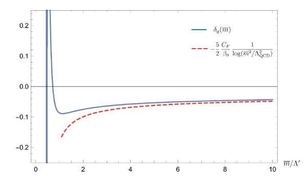
Figure 1: $\delta_{g}$ vs. $\overline{m}/\Lambda^{\prime}$ in the case that the number of light quark flavors is zero, i.e., $\beta_{0}=11$. Dashed line shows the leading asymptotic term for large $\overline{m}$, eq. (19).

On the other hand, $\delta_{G}$ includes IR renormalons, hence the series is asymptotic (convergence radius is zero). We can separate a genuine UV part and IR sensitive part of $\delta_{G}$ by the CD prescription. By appropriately subtracting the UV divergence, we can write

$$\delta_{G}(\overline{m}) =\lim_{M\to\infty}\left[\int^{M^{2}}_{0}\frac{d\tau}{\pi\tau}\,{\rm Im}\,\overline{W}_{m}\!\left(\dfrac{\tau}{\overline{m}^{2}}\right)\,{\alpha_{\beta_{0}}(\tau)}-f_{\rm UV}\right]$$ (20)

$$=\int^{\infty}_{0}\frac{d\tau}{\pi\tau}\,\left[{\rm Im}\,\overline{W}_{m}\!\left(\dfrac{\tau}{\overline{m}^{2}}\right)-\frac{3C_{F}}{4\pi}\,\theta(\tau-e^{5/3}\overline{m}^{2})\right]{\alpha_{\beta_{0}}(\tau)}\,,$$ (21)

where

$$\overline{W}_{m}(s)=-\frac{C_{F}}{4\pi}\int^{1}_{0}dx\,\left[(2+2x)\log\left({x^{2}+s\,x-s-i0}\right)+2x\right]\,,$$ (22)

and

$$f_{\rm UV}=\frac{3C_{F}}{\beta_{0}}\log\left[\frac{\log(M^{2}/\Lambda^{\prime 2})}{\log(\overline{m}^{2}/\Lambda_{\rm QCD}^{2})}\right]\,.$$ (23)

In the equality of eq. (21) we have expressed $f_{\rm UV}$ in an integral form and taken the limit $M\to\infty$; $\theta(x)$ denotes the unit step function. $\overline{W}_{m}(s)$ can be expressed in terms of elementary functions. By expanding eq. (20) or (21) in $\alpha_{s}(\overline{m})$ one can check that eq. (16) is reproduced.

Now we can apply the CD prescription to the first term of eq. (20). We introduce a factorization scale $\mu_{f}(\gg\Lambda^{\prime})$ and restrict the integral region as $(0,M^{2})\to(\mu_{f}^{2},M^{2})$. Then the integral becomes well defined avoiding the singularity of $\alpha_{\beta_{0}}(\tau)$. We can separate the integral to a genuine UV part (independent of $\mu_{f}$) and IR sensitive part (dependent on $\mu_{f}$). Using the expansion of $\overline{W}_{m}$ for $|\tau/\overline{m}^{2}|\ll 1$,

$$\overline{W}_{m}=\frac{C_{F}}{4\pi}\left[4+2\pi i\left(\frac{\tau}{\overline{m}^{2}}\right)^{1/2}-3\left(\frac{\tau}{\overline{m}^{2}}\right)-\frac{3\pi i}{4}\left(\frac{\tau}{\overline{m}^{2}}\right)^{3/2}+\cdots\right]\,,$$ (24)

we obtain

$$\delta_{G,UV} \equiv\lim_{M\to\infty}\left[{\rm Im}\int^{M^{2}}_{\mu_{f}^{2}}\frac{d\tau}{\pi\tau}\,\overline{W}_{m}\!\left(\dfrac{\tau}{\overline{m}^{2}}\right)\,{\alpha_{\beta_{0}}(\tau)}-f_{\rm UV}\right]$$

$$=\delta_{G,0}(\overline{m})+\frac{C_{0}^{m}(\mu_{f})}{\overline{m}}-\frac{3C_{F}}{\beta_{0}}\frac{\Lambda^{\prime 2}}{\overline{m}^{2}}+{\cal O}(\Lambda_{\rm QCD}^{3}/\overline{m}^{3})\,.$$ (25)

The first and third terms of the expansion are independent of $\mu_{f}$. The first term is given by

$$\delta_{G,0}(\overline{m}) =\lim_{M\to\infty}\left[\frac{4C_{F}}{\beta_{0}}+{\rm Im}\int_{C_{a}}\frac{d\tau}{\pi\tau}\,\overline{W}_{m}\!\left(\dfrac{\tau}{\overline{m}^{2}}\right)\,{\alpha_{\beta_{0}}(\tau)}-f_{\rm UV}\right]$$ (26)

$$=\frac{C_{F}}{\pi\beta_{0}}\int_{0}^{\infty}ds\,w(s)\,A\left(s\overline{m}^{2}/\Lambda^{\prime 2}\right)+\frac{3C_{F}}{\beta_{0}}\log\left[\frac{\log\left(\overline{m}^{2}/\Lambda_{\rm{QCD}}^{2}\right)}{\pi/e}\right]\,,$$ (27)

where

$$A(x)=\frac{\pi}{2}-\arctan\left[\frac{\log(x)}{\pi}\right]\,,$$ (28)

and

$$w(s)=-2+s\log s-2\left(s^{2}-2s-2\right)T(s)-\frac{3}{s}\,\theta\left(s-\frac{\Lambda^{\prime 2}}{\overline{m}^{2}}\right)\,,$$ (29)

$$T(s)=\theta(4-s)\frac{\arctan\left(\sqrt{\frac{4-s}{s}}\right)}{\sqrt{s(4-s)}}+\theta(s-4)\frac{{\rm arctanh}\left(\sqrt{\frac{s-4}{s}}\right)}{\sqrt{s(s-4)}}\,.$$ (30)

The integral contour $C_{a}$ is shown in Fig. 2(a). In eq. (27), we rotate the contour to the negative real $\tau$-axis ($\tau=e^{i\pi}\,s\,\overline{m}^{2}/\Lambda^{\prime 2}$) in order to remove the $M^{2}$ dependence between the second and third terms of eq. (26). The dependence of $\delta_{G,0}(\overline{m})$ on $\overline{m}/\Lambda^{\prime}$ is shown in Fig. 3. Its asymptotic form is given by

$$\delta_{G,0}(\overline{m}) \to\frac{13}{2}\,\frac{C_{F}}{\beta_{0}}\,\frac{1}{\log(\overline{m}^{2}/\Lambda^{\prime 2})}~{}~{}~{}\mbox{for}~{}~{}~{}\overline{m}/\Lambda^{\prime}\gg 1\,.$$ (31)

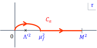
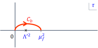
(a)                                                            (b)

Figure 2: Integral contours in the complex $\tau$-plane shown by red lines. The pole position of $\alpha_{\beta_{0}}(\tau)$ is also shown.

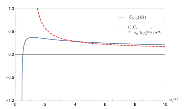
Figure 3: $\delta_{G,0}$ vs. $\overline{m}/\Lambda^{\prime}$ in the case that the number of light quark flavors is zero. Dashed line shows the leading asymptotic term for large $\overline{m}$, eq. (31).

The second term of eq. (25) depends on $\mu_{f}$. If we multiply the term by $\overline{m}$, it is independent of $\overline{m}$ and is given by

$$C_{0}^{m}(\mu_{f})=-\frac{C_{F}}{2\pi}\,{\rm Re}\int_{C_{b}}\frac{d\tau}{\sqrt{\tau}}\,\alpha_{\beta_{0}}(\tau)\,,$$ (32)

where the integral contour $C_{b}$ is shown in Fig.  2(b). The corresponding term in the QCD potential has exactly the form such that $2C_{0}^{m}(\mu_{f})+C_{0}^{V}(\mu_{f})=0$ in the CD prescription [5], showing the cancellation of renormalons in the $r$ and $\overline{m}$-independent part of $E_{\rm tot}(r)$; c.f., eqs. (1) and (2).

Thus, $\Delta M_{0}(\overline{m})$ in eq. (2) is given by

$$\Delta M_{0}(\overline{m})=(\delta_{g}+\delta_{G,0})\cdot\overline{m}\,.$$ (33)

The asymptotic form is determined by the sum of eqs. (19) and (31) and reads

$$\Delta M_{0}(\overline{m}) \to\,\frac{4C_{F}}{\beta_{0}}\,\frac{\overline{m}}{\log(\overline{m}^{2}/\Lambda_{\rm QCD}^{2})}~{}~{}~{}\mbox{for}~{}~{}~{}\overline{m}/\Lambda_{\rm QCD}\gg 1\,.$$ (34)

It agrees with the requirement by RG for the leading asymptotic behavior of the mass difference $m_{\rm pole}-\overline{m}(\overline{m})$.

As can be seen from Figs. 1 and 3 (see also Fig. 4 below), the behavior of $\Delta M_{0}(\overline{m})$ at $\overline{m}\gtrsim\Lambda^{\prime}$ is consistent with the expectation that it is proportional to $\overline{m}$ with logarithmic corrections at large $\overline{m}$. At small $\overline{m}(\lesssim\Lambda^{\prime}$), however, $\Delta M_{0}(\overline{m})$ has an oscillatory behavior. This feature is absent in the corresponding expansions of the static potential $V_{\rm QCD}(r)$ and the Adler function [6, 7], whose radiative corrections are dominated by those in Euclidean regions. The oscillatory behavior may reflect the fact that in the pole mass the self-energy corrections close to the on-shell quark configuration involve time-like kinematics. In any case, since this behavior can be concealed by ${\cal O}(\Lambda_{\rm QCD}^{3}/\overline{m}^{2})$ renormalon uncertainties, we cannot make any definite statement about it.

The final result for the genuinely UV (renormalon-free) part of the total energy is given by

$$E_{\rm tot}(r)=V_{C}(r)+C_{1}^{V}r+2\left[\overline{m}+\Delta M_{0}(\overline{m})+\frac{C_{1}^{m}}{\overline{m}}\right]+{\cal O}(\Lambda_{\rm QCD}^{3}r^{2},\,\Lambda_{\rm QCD}^{3}/\overline{m}^{2})\,.$$ (35)

with

$$C_{1}^{m}=-\frac{3C_{F}}{\beta_{0}}\Lambda^{\prime 2}\,.$$ (36)

The $\overline{m}$-dependent part, $\Delta M_{0}(\overline{m})+{C_{1}^{m}}/{\overline{m}}$, is shown in Fig. 4 as a function of $\overline{m}/\Lambda^{\prime}$. We see that the contribution of the $C_{1}^{m}/\overline{m}$ term quickly diminishes at $\overline{m}/\Lambda^{\prime}\gtrsim 2$. For completeness we also list the known results for $V_{C}(r)$ and $C_{1}^{V}$ in the large-$\beta_{0}$ approximation:

$$V_{C}(r)=-\frac{4C_{F}}{\beta_{0}r}\int_{0}^{\infty}\!\!dt\,{e^{-t}}\,A\left(t^{2}/(\Lambda^{\prime 2}r^{2})\right)\,,$$ (37)

$$C_{1}^{V}=\frac{2\pi C_{F}}{\beta_{0}}\Lambda^{\prime 2}\,.$$ (38)

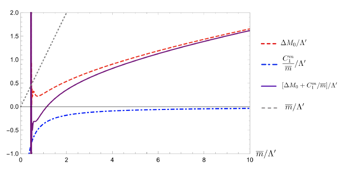
Figure 4: $[\Delta M_{0}+{C_{1}^{m}}/{\overline{m}}]/\Lambda^{\prime}$ vs. $\overline{m}/\Lambda^{\prime}$ in the case that the number of light quark flavors is zero (purple solid line). Individual terms are shown in red dashed ($\Delta M_{0}/\Lambda^{\prime}$) and blue dot-dashed (${C_{1}^{m}}/({\overline{m}}\Lambda^{\prime})$) lines. For comparison, $\overline{m}/\Lambda^{\prime}$ is shown as a gray dotted line.

Let us present some speculation. $\Delta M_{0}(\overline{m})$ consists of $\overline{m}\cdot\delta_{g}$, the part which can be expanded in the Taylor series in $\alpha_{s}(\overline{m})$, and $\overline{m}\cdot\delta_{G,0}$, the part which cannot be expanded in the Taylor series in $\alpha_{s}(\overline{m})$ [expansion in $1/\log(\overline{m}/\Lambda_{\rm QCD})$ is asymptotic]. The former is tightly connected with the renormalization of the $\overline{\rm MS}$ mass and is intrinsic to this mass scheme. The latter originates from the UV part of the asymptotic series $\sim G_{n+1}\cdot n!$, and hence is likely to be tied to the pole mass, irrespective of the definition of the short-distance mass.

There is no $r$-independent or $\overline{m}$-independent term proportional to $\Lambda_{\rm QCD}$ in the latter part of $E_{\rm tot}(r)$ in expansions in $r$ and $1/\overline{m}$. This would be natural with regard to the fact that the size of a heavy quarkonium bound state is small compared to ordinary hadrons. As a whole we consider that the expression of $E_{\rm tot}(r)$ in eq. (35) has a natural form: It includes only UV contributions; It is composed of the part which conforms with power expansions in $1/\overline{m}$ and $r$ ($\delta_{G,0}$, $C_{1}^{m}$, $V_{C}$ and $C_{1}^{V}$) and the part which can be expanded in the Taylor series in powers of $\alpha_{s}(\overline{m})\sim 1/\log(\overline{m}/\Lambda_{\rm QCD})$ whose expansion coefficients originate from the UV divergences of the short-distance mass ($\delta_{g}$). In turn, this can be taken as an evidence that we have chosen a sensible scheme for separating the UV and IR contributions and performing expansions in $r$ and $1/\overline{m}$.

Finally we comment on possible existence of ${\cal O}(\Lambda_{\rm QCD}^{2}/m)$ renormalon contained in the pole mass, whose properties are as yet not well known. Known properties are as follows [19]. (a) It is induced by the non-relativistic kinetic energy operator $\vec{D}^{2}/(2m)$; (b) It is not forbidden by any symmetry, and corresponds to the singularity at $u=1$ in the Borel plane; (c) It does not appear in the large-$\beta_{0}$ approximation. Thus, it could affect the computable part of $E_{\rm tot}(r)$ beyond the large-$\beta_{0}$ approximation. We leave this issue to future study.

References

[1]
A. Pineda,
“Heavy Quarkonium And Nonrelativistic Effective Field Theories,”
Ph.D. Thesis (1998).
[2]
A. H. Hoang, M. C. Smith, T. Stelzer and S. Willenbrock,
“Quarkonia and the pole mass,”
Phys. Rev. D 59, 114014 (1999);
[arXiv:hep-ph/9804227].
[3]
M. Beneke,
“A quark mass definition adequate for threshold problems,”
Phys. Lett. B 434, 115 (1998).
[arXiv:hep-ph/9804241].
[4]
Y. Sumino,
“QCD potential as a ‘Coulomb plus linear’ potential,”
Phys. Lett. B 571, 173 (2003)
[hep-ph/0303120].
[5]
Y. Sumino,
“‘Coulomb + linear’ form of the static QCD potential in operator product expansion,”
Phys. Lett. B 595, 387 (2004)
[hep-ph/0403242].
[6]
Y. Sumino,
“Static QCD potential at : Perturbative expansion and operator-product expansion,”
Phys. Rev. D 76, 114009 (2007)
[hep-ph/0505034].
[7]
G. Mishima, Y. Sumino and H. Takaura,
“UV contribution and power dependence on of Adler function,”
Phys. Lett. B 759, 550 (2016)
[arXiv:1602.02790 [hep-ph]].
[8]
G. Mishima, Y. Sumino and H. Takaura,
“Subtracting infrared renormalons from Wilson coefficients: Uniqueness and power dependences on ,”
Phys. Rev. D 95, no. 11, 114016 (2017)
[arXiv:1612.08711 [hep-ph]].
[9]
N. Brambilla, A. Pineda, J. Soto and A. Vairo,
“Effective field theories for heavy quarkonium,”
Rev. Mod. Phys. 77, 1423 (2005)
[hep-ph/0410047].
[10]
H. Takaura, T. Kaneko, Y. Kiyo and Y. Sumino,
“Determination of from static QCD potential with renormalon subtraction,”
Phys. Lett. B 789, 598 (2019)
[arXiv:1808.01632 [hep-ph]].
[11]
H. Takaura, T. Kaneko, Y. Kiyo and Y. Sumino,
“Determination of from static QCD potential: OPE with renormalon subtraction and Lattice QCD,”
arXiv:1808.01643 [hep-ph].
[12]
G. Corcella,
“The top-quark mass: challenges in definition and determination,”
arXiv:1903.06574 [hep-ph].
[13]
Y. Kiyo, G. Mishima and Y. Sumino,
“Strong IR Cancellation in Heavy Quarkonium and Precise Top Mass Determination,”
JHEP 1511, 084 (2015)
[arXiv:1506.06542 [hep-ph]].
[14]
A. Pineda,
“Determination of the bottom quark mass from the Upsilon(1S) system,”
JHEP 0106, 022 (2001)
[hep-ph/0105008].
[15]
C. Ayala, G. Cvetic and A. Pineda,
“The bottom quark mass from the system at NNNLO,”
JHEP 1409, 045 (2014)
[arXiv:1407.2128 [hep-ph]].
[16]
M. Neubert,
“Scale setting in QCD and the momentum flow in Feynman diagrams,”
Phys. Rev. D 51, 5924 (1995)
[hep-ph/9412265].
[17]
M. Beneke and V. M. Braun,
“Naive non-abelianization and resummation of fermion bubble chains,”
Phys. Lett. B 348 (1995) 513
[hep-ph/9411229].
[18]
P. Ball, M. Beneke and V. M. Braun,
“Resummation of corrections in QCD: Techniques and applications to the tau hadronic width and the heavy quark pole mass,”
Nucl. Phys. B 452, 563 (1995)
[hep-ph/9502300].
[19]
M. Neubert,
“Exploring the invisible renormalon: Renormalization of the heavy quark kinetic energy,”
Phys. Lett. B 393, 110 (1997)
[hep-ph/9610471].
[20]
Y. Kiyo and Y. Sumino,
“Off-shell suppression of renormalons in nonrelativistic QCD bound states,”
Phys. Lett. B 535, 145 (2002)
[hep-ph/0110277].