Decay $X(3872)\to\pi^{0}\pi^{+}\pi^{-}$ and $S$-wave $D^{0}\bar{D}^{0}\to\pi^{+}\pi^{-}$ scattering length

Abstract

The isospin-breaking decay $X(3872)\to(D^{*}\bar{D}+\bar{D}^{*}D)\to\pi^{0}D\bar{D}\to\pi^{0}\pi^{+}\pi^{-}$ is discussed. In its amplitude there is a triangle logarithmic singularity, due to which the dominant contribution to $BR(X(3872)\to\pi^{0}\pi^{+}\pi^{-})$ comes from the production of the $\pi^{+}\pi^{-}$ system in a narrow interval of the invariant mass $m_{\pi^{+}\pi^{-}}$ near the value of $2m_{D^{0}}\approx 3.73$ GeV. The analysis shows that $BR(X(3872)\to\pi^{0}\pi^{+}\pi^{-})$ can be expected at the level of $10^{-3}$–$10^{-4}$. This estimate includes, in particular, the assumption that the $S$-wave inelastic scattering length $|\alpha^{\prime\prime}_{D^{0}\bar{D}^{0}\to\pi^{+}\pi^{-}}|\approx 1/(2m_{D^{*+}})\approx 0.25\ \mbox{GeV}^{-1}$.

I Introduction

The state $X(3872)$ [or $\chi_{c1}(3872)$ PDG18 ] was first observed in 2003 by the Belle Collaboration in the process $B\to K(X(3872)\to\pi^{+}\pi^{-}J/\psi)$ Cho03 . Then it was observed in many other experiments in other processes and decay channels PDG18 . The $X(3872)$ is a narrow resonance in non-$(D^{*0}\bar{D}^{0}+\bar{D}^{*0}D^{0})$ decay channels, $\Gamma_{X}<1.2$ MeV Cho11 , and its mass coincides practically with the $D^{*0}\bar{D}^{0}$ threshold PDG18 . It has the quantum numbers $I^{G}(J^{PC})=0^{+}(1^{++})$ PDG18 ; Aub05 ; Aai15 . In addition to decay into $\pi^{+}\pi^{-}J/\psi$ Cho03 ; Aai13 ; Abl14 , the $X(3872)$ also decays into $\omega J/\psi$ Abe05 ; Amo10 ; Abl19 ; FN1 , $D^{*0}\bar{D}^{0}+c.c.$ Gok06 ; Aus10 , $\gamma J/\psi$ Aub09 ; Bha11 ; Aai14 , $\gamma\psi(2S)$ Aub09 ; Bha11 ; Aai14 , and $\pi^{0}\chi_{c1}(1P)$ Ab19 ; FN2 . The nature of $X(3872)$ remains the subject of much discussion; see, for example, Refs. Aub09 ; Bha11 ; Aai14 ; FN2 ; Ab19 ; Che16 ; Esp16 ; Leb17 ; Ali17 ; Ols18 ; Guo18 ; AR14 ; AR15 ; AR16 ; A16 ; A17 ; Ach18 ; Mut ; Sun ; Fer . Of course, new experiments will allow making a more definite choice between different interpretations.

The search for $X(3872)$ in decay channels that do not contain charmed particles or charmonium states [i.e., in channels other than $D^{*0}\bar{D}^{0}+c.c.$, $D^{0}\bar{D}^{0}\pi^{0}$, $\pi^{+}\pi^{-}J/\psi$, $\omega J/\psi$, $\gamma J/\psi$, $\gamma\psi(2S)$, $\pi^{+}\pi^{-}\eta_{c}(1S)$, $\pi^{+}\pi^{-}\chi_{c1}(1P)$, and $\pi^{0}\chi_{c1}(1P)$] is of great interest PDG18 ; Ach18 ; Mut ; Sun ; Fer ; AR15 ; AR16 ; A16 ; A17 ; AR14 ; Aai17 ; Bar18 . For example, the $c\bar{c}=\chi_{c1}(2P)$ scenario predicts a significant number of various two gluon decays $X(3872)\to(\mbox{gluon}+\mbox{gluon})\to\mbox{light\ hadrons}$ Ach18 ; AR15 ; AR16 ; A16 ; A17 . The situation here is qualitatively the same as for the decays $\chi_{c1}(1P)\to(\mbox{gluon}+\mbox{gluon})\to\mbox{light\ hadrons}$. In this way, only one channel has been explored so far PDG18 . Namely, the LHCb Collaboration undertook a search for the decay $X(3872)\to p\bar{p}$, which resulted in the following restriction Aai17 :

$$\frac{BR(B^{+}\to X(3872)K^{+})\times(BR(X(3872)\to p\bar{p})}{BR(B^{+}\to J/\psi K^{+})\times(BR(J/\psi\to p\bar{p})}$$

$$<0.25\times 10^{-2}.\qquad\qquad\qquad$$ (1)

Hence, in view of $BR(B^{+}\to J/\psi K^{+})\times(BR(J/\psi\to p\bar{p})\approx 2.14\times 10^{-6}$ PDG18 and $0.9\times 10^{-4}<BR(B^{+}\to X(3872)K^{+})<2.7\times 10^{-4}$ PDG18 ; Yua , it follows that

$$BR(X(3872)\to p\bar{p})<0.6\times 10^{-4}.$$ (2)

Taking into account a sizable contribution of the $D^{*0}\bar{D}^{0}+\bar{D}^{*0}D^{0}$ channel (and also the channels containing the charmonium states) to the $X(3872)$ decay rate, one can conclude that the above relation is in satisfactory agreement (at least not in contradiction) with what is observed in the decays of the $\chi_{c1}(1P)$ meson: $BR(\chi_{c1}(1P)\to p\bar{p})=(7.60\pm 0.34)\times 10^{-5}$ PDG18 . Note that the $\chi_{c1}(1P)$ has only one decay into $\gamma J/\psi$ containing $c\bar{c}$ quarks in the final state. It is also proposed to investigate the $X(3872)$ coupling to the $p\bar{p}$ channel in the reaction $p\bar{p}\to X(3872)\to\pi^{+}\pi^{-}J/\psi$ with the PANDA detector Bar18 .

We propose to obtain an experimental limit on the probability of the decay $X(3872)\to\pi^{0}\pi^{+}\pi^{-}$ and, if lucky, to register this decay. According to our estimate, the branching ratio of the decay $X(3872)\to\pi^{0}\pi^{+}\pi^{-}$ can be expected at the level of $10^{-3}$–$10^{-4}$ due to the transition mechanism $X(3872)\to(D^{*}\bar{D}+\bar{D}^{*}D)\to\pi^{0}D\bar{D}\to\pi^{0}\pi^{+}\pi^{-}$. In this case, the main contribution to $BR(X(3872)\to\pi^{0}\pi^{+}\pi^{-})$ comes from the production of $\pi^{+}\pi^{-}$ pairs in a narrow interval of the invariant mass $m_{\pi^{+}\pi^{-}}$ near the value of $2m_{D^{0}}\approx 3.73$ GeV.

As for the nature of X(3872), our calculations implicitly imply for this state the conventional $c\bar{c}$ nature, i.e., that it is a compact charmonium state similar to the states $\chi_{c1}(1P)$, $\psi(2S)$, $\psi(3770)$, and so on, and to describe its decays one can use the effective phenomenological Lagrangian approach AR14 ; AR15 ; AR16 ; A16 ; A17 ; Ach18 .

II Estimate of $BR(X(3872)\to\pi^{0}\pi^{+}\pi^{-})$

The decay $X(3872)\to(D^{*0}\bar{D}^{0}+\bar{D}^{*0}D^{0})\to\pi^{0}D^{0}\bar{D}^{0}$ (see Fig. 1) is one of the main decay channels of the $X(3872)$ resonance PDG18 . Because of the final state interaction among $D^{0}$ and $\bar{D}^{0}$ mesons, i.e., due to the $S$-wave transition $D^{0}\bar{D}^{0}\to\pi^{+}\pi^{-}$, the isospin breaking decay $X(3872)\to(D^{*0}\bar{D}^{0}+\bar{D}^{*0}D^{0})\to\pi^{0}D^{0}\bar{D}^{0}\to\pi^{0}\pi^{+}\pi^{-}$ is induced (see Fig. 2).

The amplitudes of such triangle diagrams, as in Fig. 2, may contain logarithmic singularities that can produce some enhancement in the mass spectra. The conditions for the appearance of such singularities in the physical region of the reaction were repeatedly deduced in various forms and discussed in the literature; see, for example, Refs. KSW58 ; Lan59 ; FN64 ; Val64 ; Ait64 ; CN65 ; Mik15 ; Liu16 ; Bay16 and also the very recent work Guo19 . For the considered mechanism of the $X\to\pi^{0}\pi^{+}\pi^{-}$ decay, these conditions are reduced to the following relations.

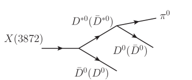
Figure 1: The diagram of the decay $X(3872)\to D^{0}\bar{D}^{0}\pi^{0}$. The four-momenta of $X(3872)$, $D^{0}$, $\bar{D}^{0}$, and $\pi^{0}$ are, respectively, $p_{1}$, $p_{D}$, $p_{\bar{D}}$, and $p_{\pi}$; the four-momenta of the intermediate $D^{*0}$ and $\bar{D}^{*0}$ are $k_{1}$ and $k_{2}$, respectively.

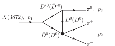
Figure 2: The diagram of the decay $X(3872)\to(D^{*0}\bar{D}^{0}+\bar{D}^{*0}D^{0})\to\pi^{0}D^{0}\bar{D}^{0}\to\pi^{0}\pi^{+}\pi^{-}$. In the $X(3872)$ mass region, all intermediate particles in the triangle loop can be near or directly on the mass shell. As a consequence, a logarithmic singularity in the imaginary part of the amplitude emerges in the hypothetical case of the stable $D^{*0}$ meson when the conditions (II) and (II) are fulfilled. The four-momenta of corresponding particles are denoted as $p_{1}$, $p_{2}$, and $p_{3}$; $p_{1}^{2}=s_{1}$ is the squared invariant mass of the $X(3872)$ resonance or of the final $\pi^{0}\pi^{+}\pi^{-}$ system; $p_{2}^{2}=s_{2}=m^{2}_{\pi^{+}\pi^{-}}$ is the squared invariant mass of the final $\pi^{+}\pi^{-}$ system; and $p_{3}^{2}=m^{2}_{\pi^{0}}$.

If the virtual invariant mass squared of the $X(3872)$ resonance $s_{1}$ falls in the range

$$2(m^{2}_{D^{*0}}+m^{2}_{D^{0}})-m^{2}_{\pi^{0}}=(3.87193\ \mbox{GeV})^{2}>s_{1}$$

$$>(m_{D^{*0}}+m_{D^{0}})^{2}=(3.87168\ \mbox{GeV})^{2},\qquad$$ (3)

then, in the range of the invariant mass squared of the $\pi^{+}\pi^{-}$ system $s_{2}=m^{2}_{\pi^{+}\pi^{-}}$

$$\frac{m_{D^{0}}}{m_{D^{*0}}}(m^{2}_{D^{*0}}+m^{2}_{D^{0}}-m^{2}_{\pi^{0}})+2m^{2}_{D^{0}}=(3.7299\ \mbox{GeV})^{2}$$

$$>s_{2}>4m^{2}_{D^{0}}=(3.72966\ \mbox{GeV})^{2},\qquad\qquad$$ (4)

the imaginary part of the amplitude of the diagram in Fig. 2 contains the triangle logarithmic singularity KSW58 ; Lan59 ; FN64 ; Val64 ; Ait64 ; CN65 ; Mik15 ; Liu16 ; Bay16 ; Guo19 . Below, we see that this singularity leads to the resonancelike enhancement in the $\pi^{+}\pi^{-}$ mass spectrum at $\sqrt{s_{2}}=m_{\pi^{+}\pi^{-}}\approx 2m_{D^{0}}\approx 3.73$ GeV, i.e., near the $D^{0}\bar{D}^{0}$ threshold.

The decay $X(3872)\to\pi^{0}\pi^{+}\pi^{-}$ can also be produced via the charged intermediate states, $X(3872)\to(D^{*+}D^{-}+D^{*-}D^{+})\to\pi^{0}D^{+}D^{-}\to\pi^{0}\pi^{+}\pi^{-}$ (see Fig. 3).

Figure 3: The diagram of the decay $X(3872)\to\pi^{0}\pi^{+}\pi^{-}$ corresponding to the charged intermediate state contributions, $X(3872)\to(D^{*+}D^{-}+D^{*-}D^{+})\to\pi^{0}D^{+}D^{-}\to\pi^{0}\pi^{+}\pi^{-}$.

From the isotopic symmetry for the coupling constants (C invariance of the amplitudes is implied), it follows that the contributions of the diagrams in Figs. 2 and 3 exactly compensate each other and the isospin breaking decay $X(3872)\to\pi^{0}\pi^{+}\pi^{-}$ is absent, if $m_{D^{*+}}=m_{D^{*0}}$ and $m_{D^{+}}=m_{D^{0}}$. However, the $D^{*0}\bar{D}^{0}$ and $D^{*+}D^{-}$ thresholds in the variable $\sqrt{s_{1}}$ differ by 8.23 MeV ($m_{D^{*0}}+m_{\bar{D}^{0}}=3.87168$ GeV, $m_{D^{*+}}+m_{D^{-}}=3.87991$ GeV) and the $D^{0}\bar{D}^{0}$ and $D^{+}D^{-}$ thresholds in the variable $\sqrt{s_{2}}$ differ by 9.644 MeV ($2m_{D^{0}}=3.72966$ GeV, $2m_{D^{\pm}}=3.73930$ GeV). Therefore, in the region of the variables $\sqrt{s_{1}}$ and $\sqrt{s_{2}}$ that is significant for the decay $X(3872)\to\pi^{0}\pi^{+}\pi^{-}$ (i.e., for $\sqrt{s_{1}}\approx m_{X}\approx m_{D^{*0}}+m_{\bar{D}^{0}}$, where $m_{X}$ is the nominal mass of the $X(3872)$ equal to 3.87169 GeV PDG18 , and $\sqrt{s_{2}}\approx 2m_{\bar{D}^{0}}\approx 3.73$ GeV), the contributions from the neutral (see Fig. 2) and charged (see Fig. 3) intermediate states weakly compensate each other and the contribution of the diagram in Fig. 2 dominates.

We write the differential probability for the decay of the virtual state $X(3872)$ to $\pi^{0}\pi^{+}\pi^{-}$ in the form

$$\frac{d^{2}BR(X\to\pi^{0}\pi^{+}\pi^{-};s_{1},s_{2})}{d\sqrt{s_{1}}d\sqrt{s_{2}}}\qquad\quad$$

$$=\frac{2\sqrt{s_{1}}}{\pi}\frac{\sqrt{s_{1}}}{|D_{X}(s_{1})|^{2}}\frac{d\Gamma(X\to\pi^{0}\pi^{+}\pi^{-};s_{1},s_{2})}{d\sqrt{s_{2}}},$$ (5)

where $D_{X}(s_{1})$ is the inverse propagator of the $X(3872)$ resonance AR14 ; AR16 ; A16 that takes into account the couplings of $X(3872)$ with the $D^{*}\bar{D}+\bar{D}^{*}D$ decay channels as well as with all non-($D^{*}\bar{D}+\bar{D}^{*}D$) decay channels; and $d\Gamma(X\to\pi^{0}\pi^{+}\pi^{-};s_{1},s_{2})/d\sqrt{s_{2}}$ is the $X\to\pi^{0}\pi^{+}\pi^{-}$ differential decay width in the variable $\sqrt{s_{2}}=m_{\pi^{+}\pi^{-}}$ caused by the sum of the diagrams in Figs. 2 and 3.

The $X(3872)$ resonance propagator constructed in Refs. AR14 ; AR16 ; A16 has good analytical and unitary properties. The inverse propagator $D_{X}(s_{1})$ has the form AR14 ; AR16 ; A16

$$D_{X}(s_{1})=m^{2}_{X}-s_{1}\qquad\qquad$$

$$+\sum_{ab}[\mbox{Re}\Pi^{ab}_{X}(m^{2}_{X})-\Pi^{ab}_{X}(s_{1})]-im_{X}\Gamma_{non},$$ (6)

where $\Gamma_{non}=\Sigma_{i}\Gamma_{i}$ is the total width of the $X(3872)$ decay to all non-$(D^{*}\bar{D}+\bar{D}^{*}D)$ channels which in the narrow region of the $X(3872)$ peak ($\Gamma_{X}<1.2$ MeV PDG18 ; Cho11 ) is approximated by a constant; $ab=D^{{}^{*}0}\bar{D}^{0}$, $\bar{D}^{{}^{*}0}D^{0}$, $D^{{}^{*}+}D^{-}$, $D^{{}^{*}-}D^{+}$. At $s_{1}>(m_{a}+m_{b})^{2}$

$$\Pi^{ab}_{X}(s_{1})=\frac{g^{2}_{A}}{16\pi}\left[\frac{m_{ab}^{(+)}m_{ab}^{(-)}}{\pi s_{1}}\ln\frac{m_{b}}{m_{a}}+\rho_{ab}(s_{1})\right.\qquad$$

$$\left.\times\left(i-\frac{1}{\pi}\,\ln\frac{\sqrt{s_{1}-m_{ab}^{(-)\,2}}+\sqrt{s_{1}-m_{ab}^{(+)\,2}}}{\sqrt{s_{1}-m_{ab}^{(-)\,2}}-\sqrt{s_{1}-m_{ab}^{(+)\,2}}}\right)\right],\ \$$ (7)

where $\rho_{ab}(s_{1})=\sqrt{s_{1}-m_{ab}^{(+)\,2}}\,\sqrt{s_{1}-m_{ab}^{(-)\,2}}/s$, $m_{ab}^{(\pm)}=m_{a}\pm m_{b}$, $m_{a}>m_{b}$,

$$\mbox{Im}\,\Pi^{ab}_{X}(s_{1})=\sqrt{s_{1}}\Gamma_{X\to ab}(s_{1})=\frac{g^{2}_{A}}{16\pi}\rho_{ab}(s_{1}),$$ (8)

and $g_{A}$ is the coupling constant of $X$ with the $D^{*0}\bar{D}^{0}$ channel. At $m_{ab}^{(-)\,2}<s_{1}<m_{ab}^{(+)\,2}$

$$\Pi^{ab}_{X}(s_{1})=\frac{g^{2}_{A}}{16\pi}\left[\frac{m_{ab}^{(+)}m_{ab}^{(-)}}{\pi s_{1}}\ln\frac{m_{b}}{m_{a}}\right.\qquad$$

$$\left.-\rho_{ab}(s_{1})\left(1-\frac{2}{\pi}\arctan\frac{\sqrt{m_{ab}^{(+)\,2}-s_{1}}}{\sqrt{s_{1}-m_{ab}^{(-)\,2}}}\right)\right],$$ (9)

where $\rho_{ab}(s_{1})$ = $\sqrt{m_{ab}^{(+)\,2}-s_{1}}\,\sqrt{s_{1}-m_{ab}^{(-)\,2}}\,/s_{1}$. If $s_{1}\leq m_{ab}^{(-)\,2}$, then $\rho_{ab}(s_{1})$ = $\sqrt{m_{ab}^{(+)\,2}-s_{1}}\,\sqrt{m_{ab}^{(-)\,2}-s_{1}}\,/s_{1}$, and

$$\Pi^{ab}_{X}(s_{1})=\frac{g^{2}_{A}}{16\pi}\left[\frac{m_{ab}^{(+)}m_{ab}^{(-)}}{\pi s_{1}}\ln\frac{m_{b}}{m_{a}}\right.\qquad\quad$$

$$\left.+\rho_{ab}(s_{1})\frac{1}{\pi}\,\ln\frac{\sqrt{m_{ab}^{(+)\,2}-s_{1}}+\sqrt{m_{ab}^{(-)\,2}-s_{1}}}{\sqrt{m_{ab}^{(+)\,2}-s_{1}}-\sqrt{m_{ab}^{(-)\,2}-s_{1}}}\right].$$ (10)

The sum of the probabilities of the $X(3872)$ decay to all modes satisfies the unitarity AR14 ; AR16 ; A16

$$BR(X\to(D^{*0}\bar{D}^{0}+c.c.))\qquad\qquad\$$

$$+BR(X\to(D^{*+}D^{-}+c.c))+\Sigma_{i}BR(X\to i)=1.$$ (11)

The coupling of the $X(3872)$ with the $D^{*0}\bar{D}^{0}$ system was introduced in Refs. AR14 ; AR15 ; AR16 ; A16 by means of the Lagrangian

$$L_{XD^{*0}\bar{D}^{0}}(x)=g_{A}X^{\mu}(D^{*0}_{\mu}\bar{D}^{0}+\bar{D}^{*0}_{\mu}D^{0})$$ (12)

and the range of possible values of the coupling constant $g^{2}_{A}/(16\pi)$ was determined from the analysis of the experimental data Cho11 ; Abe05 ; Amo10 ; Aus10 ; Aai13 ; Bha11 .

To describe the amplitudes of the $D^{*}\to D\pi^{0}$ decays, we use the expression

$$V_{D^{*}D\pi^{0}}=g_{D^{*}D\pi^{0}}(\epsilon_{D^{*}},p_{\pi^{0}}-p_{D})\,,$$ (13)

where $\epsilon_{D^{*}}$ is the polarization four-vector of the $D^{*}$ meson, $p_{\pi^{0}}$ and $p_{D}$ are the four-momenta of $\pi^{0}$ and $D$, respectively; $\,g_{D^{*+}D^{+}\pi^{0}}=-g_{D^{*0}D^{0}\pi^{0}}$.

The effective vertex of the $X(3872)\to(D^{*}\bar{D}+\bar{D}^{*}D)\to\pi^{0}D\bar{D}\to\pi^{0}\pi^{+}\pi^{-}$ transition corresponding to the sum of the diagrams in Figs. 2 and 3, in which the $\pi^{+}\pi^{-}$ system is produced in the $S$ wave, can be written as

$$V_{X\pi^{0}\pi^{+}\pi^{-}}=G_{X\pi^{0}\pi^{+}\pi^{-}}(s_{1},s_{2})(\epsilon_{X},p_{3}-p_{2})$$

$$=2\frac{\bar{g}}{16\pi}[F_{0}(s_{1},s_{2})-F_{+}(s_{1},s_{2})]\,,\qquad$$ (14)

where the invariant amplitude $G_{X\pi^{0}\pi^{+}\pi^{-}}(s_{1},s_{2})$ is used below [see, Eq. (II)] to compactly write the expression for the energy dependent differential width of the $X\to\pi^{0}\pi^{+}\pi^{-}$ decay; $\epsilon_{X}$ is the polarization four-vector of the $X(3872)$, the amplitudes $F_{0}(s_{1},s_{2})$ and $F_{+}(s_{1},s_{2})$ describe the contributions from the neutral and charged intermediate $D^{*}\bar{D}$ states, respectively, and

$$\bar{g}_{=}g_{A}\,g_{D^{*0}D^{0}\pi^{0}}\,g_{D^{0}\bar{D}^{0}\pi^{+}\pi^{-}}.$$ (15)

We assume the $S$-wave amplitudes of the processes $D^{0}\bar{D}^{0}\to\pi^{+}\pi^{-}$ and $D^{+}\bar{D}^{-}\to\pi^{+}\pi^{-}$ (entering in the amplitudes of the diagrams in Figs. 2 and 3) to be equal and approximate them in the region of the $D\bar{D}$ thresholds by an $s_{2}$-independent constant $g_{D^{0}\bar{D}^{0}\pi^{+}\pi^{-}}$.

Taking into account Eqs. (12)–(II), the amplitude $F_{0}(s_{1},s_{2})$ can be written in the form

$$F_{0}(s_{1},s_{2})=\frac{i}{\pi^{3}}\,\epsilon_{X\mu}\int\frac{\left(-g_{\mu\nu}+\frac{k_{\mu}k_{\nu}}{m^{2}_{D^{*0}}}\right)(2p_{3\nu}-k_{\nu})}{(k^{2}-m^{2}_{D^{*0}}+i\varepsilon)}\quad$$

$$\times\,\frac{d^{4}k}{((p_{1}-k)^{2}-m^{2}_{D^{0}}+i\varepsilon)((k-p_{3})^{2}-m^{2}_{\bar{D}^{0}}+i\varepsilon)}.\ \$$ (16)

The four-vector under the integral sign we transform as follows

$$\left(-g_{\mu\nu}-\frac{k_{\mu}k_{\nu}}{m^{2}_{D^{*}}}\right)(2p_{3\nu}-k_{\nu})=-2p_{3\mu}+k_{\mu}\left(m^{2}_{D^{*0}}\right.$$

$$\left.-m^{2}_{D^{0}}+m^{2}_{\pi^{0}}\right)/m^{2}_{D^{*0}}-k_{\mu}((k-p_{3})^{2}-m^{2}_{\bar{D}^{0}})/m^{2}_{D^{*0}}.\$$ (17)

This shows that after reducing the numerator and denominator in Eq. (II) by the factor $((k-p_{3})^{2}-m^{2}_{\bar{D}^{0}})$, the divergent part of the integral is proportional to $p_{1\mu}$ [i.e., the four-moment of the $X(3872)$ resonance] and does not contribute to $F_{0}(s_{1},s_{2})$ because $(\epsilon_{X},p_{1})=0$. For the numerical calculation of the amplitudes $F_{0}(s_{1},s_{2})$ in Eq. (16), we use the method developed in Refs. tHV79 ; PV79 . Note that the part of the contribution from the second term in (17), $k_{\mu}(m^{2}_{D^{*0}}-m^{2}_{D^{0}}+m^{2}_{\pi^{0}})/m^{2}_{D^{*0}}$, which after integration turns out to be proportional to $p_{3\mu}$, gives a negligible contribution to $F_{0}(s_{1},s_{2})$ in the $\sqrt{s_{1}}$ and $\sqrt{s_{2}}$ region under consideration. Thus we put

$$F_{0}(s_{1},s_{2})=-2(\epsilon_{X},p_{3})\frac{i}{\pi^{3}}\,\int\frac{d^{4}k}{(k^{2}-m^{2}_{D^{*0}}+i\varepsilon)}\quad\ \,$$

$$\times\frac{1}{((p_{1}-k)^{2}-m^{2}_{D^{0}}+i\varepsilon)((k-p_{3})^{2}-m^{2}_{\bar{D}^{0}}+i\varepsilon)}.\ \$$ (18)

The amplitude $F_{+}(s_{1},s_{2})$ is obtained from Eq. (II) by replacing the masses of neutral $D^{*}$ and $D$ mesons by the masses of their charged partners.

Using Eq. (II) we express the differential width $d\Gamma(X\to\pi^{0}\pi^{+}\pi^{-};s_{1},s_{2})/d\sqrt{s_{2}}$ in terms of the invariant amplitude $G_{X\pi^{0}\pi^{+}\pi^{-}}(s_{1},s_{2})$.

$$\frac{d\Gamma(X\to\pi^{0}\pi^{+}\pi^{-};s_{1},s_{2})}{d\sqrt{s_{2}}}\qquad\qquad\ \$$

$$=\frac{2}{3}\,\frac{|G_{X\pi^{0}\pi^{+}\pi^{-}}(s_{1},s_{2})|^{2}}{4\pi}\,\frac{p^{3}(s_{1},s_{2})}{s_{1}}\,\frac{\rho(s_{2})}{16\pi}\,\frac{2\sqrt{s_{2}}}{\pi}\,,$$ (19)

where

$$p(s_{1},s_{2})=\frac{\sqrt{s_{1}^{2}-2s_{1}(s_{2}+m^{2}_{\pi^{0}})+(s_{2}-m^{2}_{\pi^{0}})^{2}}}{2\sqrt{s_{1}}},$$ (20)

$$\rho(s_{2})=\sqrt{1-4m^{2}_{\pi^{+}}/s_{2}}.\qquad\qquad\quad$$ (21)

The width of the decay $X\to\pi^{0}\pi^{+}\pi^{-}$ as a function of $s_{1}$ has the form

$$\Gamma(X\to\pi^{0}\pi^{+}\pi^{-};s_{1})\qquad\qquad$$

$$=\int^{\sqrt{s_{1}}-m_{\pi}^{0}}_{2m_{\pi^{+}}}\frac{d\Gamma(X\to\pi^{0}\pi^{+}\pi^{-};s_{1},s_{2})}{d\sqrt{s_{2}}}d\sqrt{s_{2}}\,,$$ (22)

and the probability of this decay is given by the expression

$$BR(X\to\pi^{0}\pi^{+}\pi^{-})\qquad\qquad\$$

$$=\int^{\infty}_{3m_{\pi}}\frac{2\sqrt{s_{1}}}{\pi}\,\frac{\sqrt{s_{1}}\Gamma(X\to\pi^{0}\pi^{+}\pi^{-};s_{1})}{|D_{X}(s_{1})|^{2}}d\sqrt{s_{1}}\,.$$ (23)

Equations (II) and (II) indicate the kinematically allowable limits of integration. In fact, the main contributions in Eqs. (II) and (II) are concentrated in much smaller intervals.

We now estimate the coupling constants $g_{D^{*0}D^{0}\pi^{0}}$ and $g_{D^{0}\bar{D}^{0}\pi^{+}\pi^{-}}$.

For the total decay width of the $D^{*0}$ meson, only its upper limit is known so far: $\Gamma_{D^{*0}}<2.1$ MeV PDG18 . On the other hand, the total decay width of the $D^{*+}$ meson and the branching ratio of the $D^{*+}\to(D\pi)^{+}$ decay are well known PDG18 : $\Gamma_{D^{*+}}\approx 83.6$ keV, $BR(D^{*+}\to(D\pi)^{+})\approx 98.4\%$. Assuming the isotopic symmetry for the coupling constants $g_{D^{*}D\pi}$, we have

$$\frac{m^{2}_{D^{*0}}\Gamma_{D^{*0}\to D^{0}\pi^{0}}}{p^{3}_{D^{0}\pi^{0}}}=\frac{m^{2}_{D^{*+}}\Gamma_{D^{*+}\to(D\pi)^{+}}}{2p^{3}_{D^{0}\pi^{+}}+p^{3}_{D^{+}\pi^{0}}}\,,$$ (24)

where $p_{D\pi}$ denotes the momentum of the final $D$ or $\pi$ meson in the $D^{*}$ rest frame. From here we find the decay width $\Gamma_{D^{*0}\to D^{0}\pi^{0}}\approx 36\,\mbox{keV}$ and the coupling constant $g^{2}_{D^{*0}D^{0}\pi^{0}}/(4\pi)=3m^{2}_{D^{*0}}\Gamma_{D^{*0}\to D^{0}\pi^{0}}/(2p^{3}_{D^{0}\pi^{0}})\approx 2.8$. Using also the value of $BR(D^{*0}\to D^{0}\pi^{0})\approx 64.7\%$ PDG18 , we get an estimate for the total decay width of the $D^{*0}$ meson: $\Gamma_{D^{*0}}\approx 55.6$ keV. Here we note in passing the following. As the examples AK1 ; AK2 ; AK3 ; AKS15 ; AS17 ; AS18 show, the instability of the vector mesons in the intermediate states (i.e., the finiteness of their total widths) is important to take into account when estimating the contributions of logarithmic triangle singularities. In this case, $\Gamma_{D^{*0}}$ is small. Nevertheless, its accounting in the $D^{*0}$ propagator (by replacing $m^{2}_{D^{*0}}\to m^{2}_{D^{*0}}-im_{D^{*0}}\Gamma_{D^{*0}}$) noticeably smoothes the logarithmic singularity in the amplitude of the diagram in Fig. 2 and the computed width $\Gamma(X(3872)\to\pi^{0}\pi^{+}\pi^{-};m_{X})$ is reduced by approximately 30% as compared to that for $\Gamma_{D^{*0}}=0$. In a similar way, we take into account the width $\Gamma_{D^{*\pm}}$ in the $D^{*\pm}$ propagator.

The constant $g_{D^{0}\bar{D}^{0}\pi^{+}\pi^{-}}$ is associated with the annihilation cross section $\sigma_{D^{0}\bar{D}^{0}\to\pi^{+}\pi^{-}}$ at the $D^{0}\bar{D}^{0}$ threshold and with the corresponding inelastic scattering length $\alpha^{\prime\prime}_{D^{0}\bar{D}^{0}\to\pi^{+}\pi^{-}}$ by the relations:

$$\frac{k\,\sigma_{D^{0}\bar{D}^{0}\to\pi^{+}\pi^{-}}}{4\pi}=|\alpha^{\prime\prime}_{D^{0}\bar{D}^{0}\to\pi^{+}\pi^{-}}|=q\left|\frac{g_{D^{0}\bar{D}^{0}\pi^{+}\pi^{-}}}{8\pi\sqrt{s_{2}}}\right|^{2},\$$ (25)

where $k$ and $q$ are momenta of the $D^{0}$ and $\pi^{+}$ mesons, respectively, in the center-of-mass frame of the reaction $D^{0}\bar{D}^{0}\to\pi^{+}\pi^{-}$. In the $D^{0}\bar{D}^{0}$ threshold domain of interest to us, $q/s_{2}\approx 1/(4m_{D^{0}})$. At present, the values in Eq. (25), which characterizes the $S$-wave $D^{0}\bar{D}^{0}\to\pi^{+}\pi^{-}$ annihilation at rest, are completely unknown. If we naively put the inelastic scattering length $|\alpha^{\prime\prime}_{D^{0}\bar{D}^{0}\to\pi^{+}\pi^{-}}|\approx 1/(2m_{D^{*+}})\approx 1/(4\,\mbox{GeV})$ (which is in dimensionless units $m_{\pi^{+}}|\alpha^{\prime\prime}_{D^{0}\bar{D}^{0}\to\pi^{+}\pi^{-}}|\approx 0.0347$), then $|g_{D^{0}\bar{D}^{0}\pi^{+}\pi^{-}}/(8\pi)|^{2}$ is approximately equal to $\approx 1.8$. We use this value in further evaluations. It is clear that our rough estimate is related to considerations about the $D^{0}\bar{D}^{0}$ annihilation radius. An experiment will show whether this value is reasonable or not. For comparison, we note that the tree $D^{0}\bar{D}^{0}\to\pi^{+}\pi^{-}$ annihilation amplitude caused by the charged $D^{*}$ exchange leads to $|\alpha^{\prime\prime}_{D^{0}\bar{D}^{0}\to\pi^{+}\pi^{-}}|$, which is about 15 times greater than our estimate, due to the large coupling constant $g^{2}_{D^{*+}D^{0}\pi^{+}}/(4\pi)\approx 5.6$ (see note FN3 ).

Figure 4: An example of the $\pi^{+}\pi^{-}$ mass spectrum $d\Gamma(X\to\pi^{0}\pi^{+}\pi^{-};s_{1},s_{2})/d\sqrt{s_{2}}$ constructed with the use of Eq. (II) at $\sqrt{s_{1}}=m_{X}=3.87169$ GeV and $g^{2}_{A}/(16\pi)=0.25$ GeV². The solid curve corresponds to the sum of the diagrams in Figs. 2 and 3. The dashed curve shows the contribution from the diagram in Fig. 2 only. The $\sqrt{s_{2}}$ values between which [according to Eq. (4)] the amplitude of the $X(3872)\to(D^{*0}\bar{D}^{0}+\bar{D}^{*0}D^{0})\to\pi^{0}D^{0}\bar{D}^{0}\to\pi^{0}\pi^{+}\pi^{-}$ decay contains the logarithmic singularity, in the hypothetical case of the stable $D^{*0}$ meson, are shown by the dotted vertical lines. In so doing, the singularity itself is located at $\sqrt{s_{2}}=3.72982$ GeV (see note FN4 ).

Figure 5: The width $\Gamma(X\to\pi^{0}\pi^{+}\pi^{-};s_{1})$ as a function of $\sqrt{s_{1}}$. The constructed example corresponds to $g^{2}_{A}/(16\pi)=0.25$ GeV².

Figure 4 shows an example of the $\pi^{+}\pi^{-}$ mass spectrum in the decay $X(3872)\to\pi^{0}\pi^{+}\pi^{-}$, i.e., $d\Gamma(X\to\pi^{0}\pi^{+}\pi^{-};s_{1},s_{2})/d\sqrt{s_{2}}$ as a function of $\sqrt{s_{2}}$, calculated with use of Eq. (II) at $\sqrt{s_{1}}=m_{X}=3.87169$ GeV and the coupling constant of $X(3872)$ with the $D^{*0}\bar{D}^{0}$ channel $g^{2}_{A}/(16\pi)=0.25$ GeV² (other possible values for $g^{2}_{A}/(16\pi)$ are discussed below). The integration $d\Gamma(X\to\pi^{0}\pi^{+}\pi^{-};m^{2}_{X},s_{2})/d\sqrt{s_{2}}$ over $\sqrt{s_{2}}$ in the region of 35 MeV wide, i.e., from $m_{X}-m_{\pi^{0}}-0.035\mbox{ GeV}=3.70171\mbox{ GeV}$ to $m_{X}-m_{\pi^{0}}=3.73671$ GeV, results in $\Gamma(X\to\pi^{0}\pi^{+}\pi^{-};m^{2}_{X})\approx 3$ keV. However, as can be seen from Fig. 5, this is in fact the maximal value of the $X(3872)\to\pi^{0}\pi^{+}\pi^{-}$ decay width in the $X(3872)$ resonance region. The width $\Gamma(X\to\pi^{0}\pi^{+}\pi^{-};s_{1})$ is a sharply changing function of $\sqrt{s_{1}}$. Two peaks in $\Gamma(X\to\pi^{0}\pi^{+}\pi^{-};s_{1})$ located near the $D^{*0}\bar{D}^{0}$ and $D^{*+}D^{-}$ thresholds (see Fig. 5) are manifestations of the logarithmic singularities in the amplitudes of the diagrams in Fig. 2 (the left peak) and in Fig. 3 (the right peak) FN5 . The most important contribution to $BR(X\to\pi^{0}\pi^{+}\pi^{-})$ [see Eq. (II)] comes from the left peak. The right peak in $\Gamma(X\to\pi^{0}\pi^{+}\pi^{-};s_{1})$ practically does not work as it is located far on the right tail of the $X(3872)$ resonance and its contribution to $BR(X\to\pi^{0}\pi^{+}\pi^{-})$ is strongly suppressed by the $X(3872)$ propagator module squared.

Figure 6: The resonance distribution $2s_{1}/(\pi|D_{X}(s_{1})|^{2})$ at $g^{2}_{A}/(16\pi)=0.25$ GeV² and $\Gamma_{non}=1$ MeV.

We now present numerical estimates for $BR(X\to\pi^{0}\pi^{+}\pi^{-})$ using as a guide the values of $g_{A}$ obtained in Refs. AR14 ; AR16 ; A16 . Figure 6 shows an example of the resonance distribution $2s_{1}/(\pi|D_{X}(s_{1})|^{2})$ calculated at $m_{X}=3.87169$ GeV PDG18 , $g^{2}_{A}/(16\pi)=0.25$ GeV², and $\Gamma_{non}=1$ MeV. Weighting with this distribution the energy dependent width $\Gamma(X\to\pi^{0}\pi^{+}\pi^{-};s_{1})$ shown in Fig. 5, we find, according to Eq. (II), that for the above values of the parameters $BR(X\to\pi^{0}\pi^{+}\pi^{-})\approx 5\times 10^{-4}$. Estimates for $BR(X\to\pi^{0}\pi^{+}\pi^{-})$ for different values of $g^{2}_{A}/(16\pi)$ and $\Gamma_{non}$, which we vary in a fairly wide but reasonable range, are given in Table I at $m_{X}=3.87169$ GeV PDG18 .

Table 1: $BR(X((3872)\to\pi^{0}\pi^{+}\pi^{-})$ in units of $10^{-4}$ for five values of $g^{2}_{A}/(16\pi)$ and three values of $\Gamma_{non}$; $m_{X}=3.87169$ GeV.

$g^{2}_{A}/(16\pi)$ (in GeV2)	= 0.1	= 0.2	= 0.25	= 0.5	= 1.0
$\Gamma_{non}=0.5$ MeV	7.42	8.42	8.35	7.10	5.19
$\Gamma_{non}=1$ MeV	3.93	4.99	5.14	4.88	3.84
$\Gamma_{non}=2$ MeV	1.93	2.70	2.89	3.07	2.67

It is not yet clear whether the mass of the $X(3872)$ state lies slightly above or slightly below the $D^{*0}\bar{D}^{0}$ threshold. The $\pm 0.17$ MeV uncertainty that the Particle Data Group PDG18 indicates allows for both possibilities. Tables II and III show the estimates for $BR(X\to\pi^{0}\pi^{+}\pi^{-})$ at the same values of $g^{2}_{A}/(16\pi)$ and $\Gamma_{non}$ as in Table I but for $m_{X}=3.87169\pm 0.00017$ GeV.

Table 2: The same as Table I but for $m_{X}=3.87169+0.00017$ GeV.

$g^{2}_{A}/(16\pi)$ (in GeV2)	= 0.1	= 0.2	= 0.25	= 0.5	= 1.0
$\Gamma_{non}=0.5$ MeV	6.45	6.97	6.82	5.63	3.94
$\Gamma_{non}=1$ MeV	3.76	4.60	4.68	4.30	3.27
$\Gamma_{non}=2$ MeV	1.93	2.64	2.80	2.89	2.45

Table 3: The same as Table I but for $m_{X}=3.87169-0.00017$ GeV.

$g^{2}_{A}/(16\pi)$ (in GeV2)	= 0.1	= 0.2	= 0.25	= 0.5	= 1.0
$\Gamma_{non}=0.5$ MeV	8.04	11.2	12.2	14.7	16.3
$\Gamma_{non}=1$ MeV	3.91	5.57	6.08	7.37	8.20
$\Gamma_{non}=2$ MeV	1.86	2.73	3.01	3.70	4.12

III Conclusion

The above analysis shows that $BR(X(3872)\to\pi^{0}\pi^{+}\pi^{-})$ can be expected at the level of $10^{-3}$–$10^{-4}$. The dominant contribution to $BR(X(3872)\to\pi^{0}\pi^{+}\pi^{-})$ comes from the production of the $\pi^{+}\pi^{-}$ system in a narrow (no more than 20 MeV wide) interval of the invariant mass $m_{\pi^{+}\pi^{-}}$ near the value of $2m_{D^{0}}\approx 3.73$ GeV. The $\pi^{+}\pi^{-}$ events with such an invariant mass can serve as a signature of the decay $X(3872)\to(D^{*0}\bar{D}^{0}+\bar{D}^{*0}D^{0})\to\pi^{0}D^{0}\bar{D}^{0}\to\pi^{0}\pi^{+}\pi^{-}$.

The present work is partially supported by Grant No. II.15.1 of fundamental scientific researches of the Siberian Branch of the Russian Academy of Sciences, Grant No. 0314-2019-0021.

References

(1) M. Tanabashi et al. (Particle Data Group), Phys. Rev. D 98, 030001 (2018).
(2) S.-K. Choi et al. (Belle Collaboration), Phys. Rev. Lett. 91, 262001 (2003).
(3) S.-K. Choi et al. (Belle Collaboration), Phys. Rev. D 84, 052004 (2011).
(4) B. Aubert et al. (BABAR Collaboration), Phys. Rev. D 71, 031501 (2005).
(5) R. Aaij et al. (LHCb Collaboration), Phys. Rev. D 92, 011102 (2015).
(6) R. Aaij et al. (LHCb Collaboration), Phys. Rev. Lett. 110, 222001 (2013).
(7) M. Ablikim et al. (BESIII Collaboration), Phys. Rev. Lett. 112, 092001 (2014).
(8) K. Abe et al. (Belle Collaboration), arXiv:hep-ex/0505037.
(9) P. del Amo Sanchez et al. (BABAR Callaboration), Phys. Rev. D 82, 011101(R) (2010).
(10) M. Ablikim et al. (BESIII Collaboration), arXiv:1903.04695.
(11) M. Suzuki, Phys. Rev. D 72, 114013 (2005).
Note that in the channel the
meson is not observed literally, but the events
at the end of the left wing of the resonance which can else
contain the destructive or constructive interference with the
background.
(12) G. Gokhroo et al. (Belle Collaboration), Phys. Rev. Lett. 97, 162002 (2006).
(13) T. Aushev et al. (Belle Collaboration), Phys. Rev. D 81, 031103 (2010).
(14) B. Aubert et al. (BABAR Collaboration), Phys. Rev. Lett. 102 132001 (2009).
(15) V. Bhardwaj et al. (Belle Collaboration), Phys. Rev. Lett. 107, 091803 (2011).
(16) R. Aaij et al. (LHCb Collaboration), Nucl. Phys. B886, 665 (2014).
(17) M. Ablikim et al. (BESIII Collaboration), Phys. Rev. Lett. 122, 202001 (2019).
(18) Nikolay Achasov, Plenary talk at the
International Workshop on collizions from Phi to Psi, 2019,
BINP, Novosibirsk, EPJ Web Conf. 212, 02001 (2019), PhiPsi
2019, arXiv:1904.08054. Note that the BESIII experiments on the
reactions Abl14 ,
Abl19 , and
Ab19 indicate,
apparently, on the two-gluon production mechanism of :
. The isospin symmetry breaking in the
decays and
do not appear to be decisive in the
question of the nature of the X(3872) state.
(19) H.X. Chen, W. Chen, X. Liu, and S.-L. Zhu,
Phys. Rep. 639, 1 (2016).
(20) A. Esposito, A. Pilloni, and A.D. Polosa, Phys. Rep. 668, 1 (2017).
(51) N.N. Achasov and A.A. Kozhevnikov, Phys. Rev. D 49, 5773 (1994).
(52) N.N. Achasov, A.A. Kozhevnikov, and G.N. Shestakov,
Phys. Rev. D 92, 036003 (2015).
(53) N.N. Achasov and G.N. Shestakov, Nucl. Part. Phys. Proc.
287–288, 89 (2017).
(54) N.N. Achasov and G.N. Shestakov, Pisma Zh. Eksp. Teor. Fiz. 107,
292 (2018) [JETP Lett. 107, 276 (2018)].
(55) For the estimate we use the transverse propagator
that carries the unit spin off the mass
shell. So where , , are
the usual Mandelstam variables for the reaction . At the threshold , . Neglecting , we get . If the propagator is , then .
(56) The contributions of the diagrams in Figs. 2 and 3 to
the width begin to cancel each
other at just below the threshold and just
above the threshold. This practically does not occur
between the thresholds due to significantly different phases of the
neutral and charged intermediate states. The phase of the
transition amplitude changes between the
and thresholds by about 90∘,
just as is the case between the and
thresholds in the mixing amplitude AS17
or in the amplitude of the decay AS18 .
(57) The logarithmic singularities in the amplitude are at
, where , , (see, for example, Refs. Lan59 ; FN64 ; Val64 ; Bay16 ; AK1 ; AK2 ; AK3 ; AKS15 ; AS18 ). Only one solution of this equation falls
into the region defined by Eqs. (II) and (II).