Towards a Robust Aerial Cinematography Platform:
Localizing and Tracking Moving Targets in Unstructured Environments

Abstract

The use of drones for aerial cinematography has revolutionized several applications and industries that require live and dynamic camera viewpoints such as entertainment, sports, and security. However, safely controlling a drone while filming a moving target usually requires multiple expert human operators; hence the need for an autonomous cinematographer. Current approaches have severe real-life limitations such as requiring fully scripted scenes, high-precision motion-capture systems or GPS tags to localize targets, and prior maps of the environment to avoid obstacles and plan for occlusion.

In this work, we overcome such limitations and propose a complete system for aerial cinematography that combines: (1) a vision-based algorithm for target localization; (2) a real-time incremental 3D signed-distance map algorithm for occlusion and safety computation; and (3) a real-time camera motion planner that optimizes smoothness, collisions, occlusions and artistic guidelines. We evaluate robustness and real-time performance in series of field experiments and simulations by tracking dynamic targets moving through unknown, unstructured environments. Finally, we verify that despite removing previous limitations, our system achieves state-of-the-art performance.

I Introduction

Figure 1: Aerial cinematographer: a) The UAV forecasts the actor’s motion using camera-based localization, maps the environment with a LiDAR, reasons about artistic guidelines, and plans a smooth, collision-free trajectory while avoiding occlusions. b) Accumulated point cloud during field test overlaid with actor’s motion forecast (blue), desired cinematography guideline (pink), and optimized trajectory (red). c) Third-person view of scene and final drone image.

In this paper, we address the problem of autonomous cinematography using unmanned aerial vehicles (UAVs). Specifically, we focus on scenarios where an UAV must film an actor moving through an unknown environment at high speeds, in an unscripted manner. Filming dynamic actors among clutter is extremely challenging, even for experienced pilots. It takes high attention and effort to simultaneously predict how the scene is going to evolve, control the UAV, avoid obstacles and reach desired viewpoints. Towards solving this problem, we present a complete system that can autonomously handle the real-life constraints involved in aerial cinematography: tracking the actor, mapping out the surrounding terrain and planning maneuvers to capture high quality, artistic shots.

Consider the typical filming scenario in Fig 1. The UAV must accomplish a number of tasks. First, it must estimate the actor’s pose using an onboard camera and forecast their future motion. The pose estimation should be robust to changing viewpoints, backgrounds and lighting conditions. Accurate forecasting is key for anticipating events which require changing camera viewpoints. Secondly, the UAV must remain safe as it flies through through new environments. Safety requires explicit modelling of environmental uncertainty. Finally, the UAV must capture high quality videos which require maximizing a set of artistic guidelines. The key challenge is that all these tasks must be done in real-time under limited onboard computational resources.

There is a rich history of work in autonomous aerial filming that tackles parts of the challenges. For instance, several works focus on artistic guidelines [1, 2, 3, 4] but often rely on perfect actor localization through high-precision RTK GNSS or motion-capture systems. Additionally, while the majority of work in the area deals with collisions between UAV and actors[2, 1, 5], the environment is not factored in. While there are several successful commercial products, they too have certain limitations to either low speed and low clutter regimes (e.g. DJI Mavic [6]) or shorter planning horizons (e.g. Skydio R1 [7]). Even our previous work [8], despite handling environmental occlusions and collisions, assumes a prior elevation map and uses GPS to localize the actor. Such simplifications impose restrictions on the diversity of real-life scenarios that these systems can handle.

We address these challenges by building upon previous work that formulates the problem as an efficient real-time trajectory optimization [8]. In this work we make a key observation: we don’t need prior ground-truth information about the scene; our onboard sensors suffice to attain good performance. However, sensor data is noisy and needs to be processed in real-time; therefore we develop robust and efficient algorithms. To localize the actor, we use a visual tracking system. To map the environment, we use a long-range LiDAR and process it incrementally to build a signed distance field of the environment. Combining both methods, we can plan over long horizons in unknown environments to film fast dynamic actors according to artistic guidelines. In summary, our main contributions in this paper are threefold:

1. We develop an incremental signed distance transform algorithm for large-scale real-time environment mapping (Section IV-B);

2. We develop a complete system for autonomous cinematography that includes visual actor localization, online mapping, and efficient trajectory optimization that can deal with noisy measurements (Section IV);

3. We offer extensive quantitative and qualitative performance evaluations of our system both in simulation and field tests, while also comparing performance changes with scenarios with full map and actor knowledge (Section V).

II Problem Formulation

The overall task is to control a UAV to film an actor who is moving through an unknown environment. We formulate this as a trajectory optimization problem where the cost function measures shot quality, environmental occlusion of the actor, jerkiness of motion and safety. This cost function depends on the environment and the actor, both of which must be sensed on-the-fly. The changing nature of environment and actor trajectory also demands re-planning at a high frequency.

Let $\xi_{q}:[0,t_{f}]\rightarrow^{3}\times SO(2)$ be the trajectory of the UAV, i.e., $\xi_{q}(t)=\{x(t),y(t),z(t),\psi_{q}(t)\}$ . Let $\xi_{a}:[0,t_{f}]\rightarrow^{3}\times SO(2)$ be the trajectory of the actor, $\xi_{a}(t)=\{x(t),y(t),z(t),\psi_{a}(t)\}$. The state of the actor, as sensed by onboard cameras, is fed into a prediction module that computes $\xi_{a}$ (Section IV-A).

Let grid $\mathcal{G}:^{3}\rightarrow$ be a voxel occupancy grid that maps every point in space to a probability of occupancy. Let $\mathcal{M}:^{3}\rightarrow$ be the signed distance values of a point to the nearest obstacle. Positive sign is for points in free space, and negative sign is for points either in occupied or unknown space, which we assume to be potentially inside an obstacle. The UAV senses the environment with the onboard LiDAR, updates grid $\mathcal{G}$, and then updates $\mathcal{M}$ (Section IV-B).

We briefly touch upon the four components of the cost function $J\left(\xi_{q}\right)$ (refer to Section IV-C for mathematical expressions). The objective is to minimize $J\left(\xi_{q}\right)$ subject to initial boundary constraints $\xi_{q}(0)$.

1. Smoothness $J_{\mathrm{smooth}}\left(\xi_{q}\right)$: Penalizes jerky motions that may lead to camera blur and unstable flight;

2. Shot quality $J_{\mathrm{shot}}\left(\xi_{q},\xi_{a}\right)$: Penalizes poor viewpoint angles and scales that deviate from the artistic guidelines

3. Safety $J_{\mathrm{obs}}\left(\xi_{q},\mathcal{M}\right)$: Penalizes proximity to obstacles that are unsafe for the UAV.

4. Occlusion $J_{\mathrm{occ}}\left(\xi_{q},\xi_{a},\mathcal{M}\right)$: Penalizes occlusion of the actor by obstacles in the environment.

$$J\left(\xi_{q}\right) =\begin{bmatrix}1&\lambda_{1}&\lambda_{2}&\lambda_{3}\end{bmatrix}\begin{bmatrix}J_{\mathrm{smooth}}\left(\xi_{q}\right)\\ J_{\mathrm{shot}}\left(\xi_{q},\xi_{a}\right)\\ J_{\mathrm{obs}}\left(\xi_{q},\mathcal{M}\right)\\ J_{\mathrm{occ}}\left(\xi_{q},\xi_{a},\mathcal{M}\right)\end{bmatrix}$$ (1)

$$\xi_{q}^{*} =\underset{}{\operatorname*{arg\,min}}\quad J\left(\xi_{q}\right),\quad\text{s.t.}\;\xi_{q}(0)=\{x_{0},y_{0},z_{0},\psi_{0}\}$$

The solution $\xi_{q}^{*}$ is then tracked by the UAV.

III Related Work

Virtual cinematography

Camera control in virtual cinematography has been extensively examined by the computer graphics community, as reviewed by [9]. These methods tend to reason about the utility of a viewpoint in isolation, following artistic principles and composition rules [10, 11] and employ either optimization-based approaches to find good viewpoints, or reactive approaches to track the virtual actor. The focus is typically on through-the-lens control where a virtual camera is manipulated while maintaining focus on certain image features [12, 13, 14, 15]. However, virtual cinematography is free of several real-world limitations such as robot physics constraints and assumes full map knowledge.

Autonomous aerial cinematography

Several contributions on aerial cinematography focus on keyframe navigation. [16, 17, 18, 19, 20] provide user interface tools for re-timing and connecting static aerial viewpoints for dynamically feasible and visually pleasing trajectories. [21] use key-frames defined on the image itself instead of world coordinates.

Other works focus on tracking dynamic targets, and employ a diverse set of techniques for actor localization and navigation. For example, [5, 22] detect the skeleton of targets from visual input, while others approaches rely on off-board actor localization methods from either motion-capture systems or GPS sensors [1, 3, 2, 4, 8]. These approaches have a varying level of complexity: [8, 4] can avoid obstacles and occlusions with the environment and with actors, while other approaches only handle collisions and occlusions caused by actors. We also observe distinct trajectory generation methods randing from trajectory optimization to search-based planners. In Table III we summarize different contributions, also differentiating onboard versus off-board computing systems. It is important to notice that prior to our current work, none of the previous approaches provided a solution for online environment mapping.

TABLE I: Comparison of dynamic aerial cinematography systems

0cmRef	0.6cmOnline
map

& 0.6cmActor localiz. 0.9cmOnboard comp. 0cmAvoids occl. 0cmAvoids obst. 0.6cmOnline plan [3] $\times$ $\times$ $\times$ $\times$ $\times$ ✓ [1] $\times$ $\times$ $\times$ $\times$ Actor ✓ [2] $\times$ $\times$ $\times$ Actor Actor ✓ [4] $\times$ $\times$ $\times$ ✓ ✓ ✓

[22] $\times$ ✓ ✓ $\times$ Actor ✓ [5] $\times$ $\checkmark$ ✓ $\times$ Actor ✓ [8] $\times$ Vision ✓ ✓ ✓ ✓ Ours ✓ ✓ ✓ ✓ ✓ ✓

Online environment mapping

Dealing with imperfect representations of the world becomes a bottleneck for viewpoint optimization in physical environments. As the world is sensed online, it is usually incrementally mapped using voxel occupancy maps [23]. To evaluate a viewpoint, methods typically raycast on such maps, which can be very expensive [24, 25]. Recent advances in mapping have led to better representations that can incrementally compute the truncated signed distance field (TSDF) [26, 27], i.e. return the distance and gradient to nearest object surface for a query. TSDFs are a suitable abstraction layer for planning approaches and have already been used to efficiently compute collision-free trajectories for UAVs [28, 29].

Visual target state estimation

Accurate object state estimation with monocular cameras is critical to many robot applications. Deep networks have shown success in detecting objects [30, 31] and estimating 3D heading [32, 33] with several efficient architectures developed specifically for mobile applications [34, 35]. However, many models do not generalize well to other tasks (e.g., aerial filming) due to data mismatch in terms of angles and scales. Our recent work in semi-supervised learning shows promise in increasing model generalizability with little labeled data by leveraging temporal continuity in training videos [36].

Our work exploits synergies at the confluence of several domains of research to develop an aerial cinematography platform that can follow dynamic targets in unknown and unstructured environments, as detailed next in our approach.

IV Approach

We now detail our approach for each sub-system of the aerial cinematography platform. At a high-level, three main sub-systems operate together: (A) Vision, required for localizing the target’s position and orientation and for recording the final UAV’s footage; (B) Mapping, required for creating an environment representation; and (C) Planning, which combines the actor’s pose and the environment to calculate the UAV trajectory. Fig. 2 shows a system diagram.

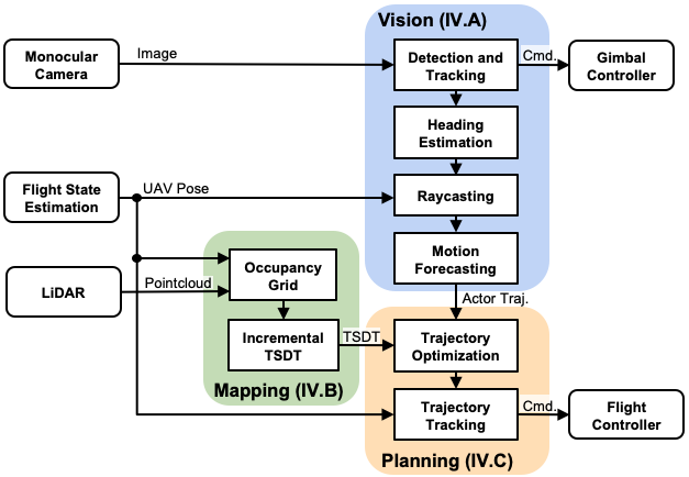
Figure 2: System architecture. Vision subsystem controls camera’s orientation and forecasts the actor trajectory $\xi_{a}$ using monocular images. Mapping receives LiDAR pointclouds to incrementally calculate a truncated signed distance transform (TSDT). Planning uses the map, the drone’s state estimation and actor’s forecast to generate trajectories for the flight controller.

IV-A Vision sub-system

We use only monocular images from the UAV’s gimbal and the UAV’s own state estimation to forecast the actor’s trajectory in the world frame. The vision sub-system counts with four main steps: actor bounding box detection and tracking, heading angle estimation; global ray-casting, and finally a filtering stage. Figure 3 summarizes the pipeline.

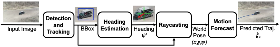
Figure 3: Vision sub-system. We detect and track the actor’s bounding box, estimate its heading, and project its pose to world coordinates. A Kalman Filter predicts the actor’s forecasted trajectory $\xi_{a}$.

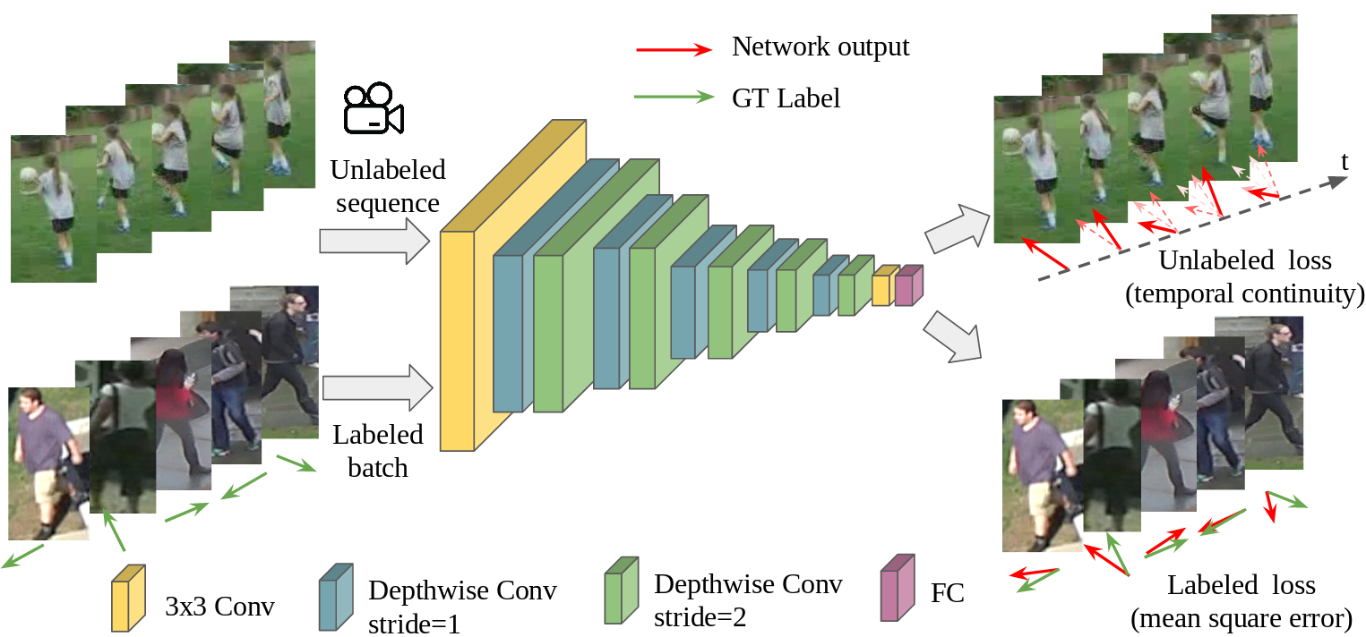
Figure 4: Heading detection network structure, from [36]. We leverage temporal continuity between frames to train a heading direction regressor with a small labeled dataset.

a) Detection and tracking: Our detection module is based on the MobileNet network architecture, due to its low memory usage and fast inference speed, which are well-suited for real-time applications on an onboard computer. We use the same network structure as detailed in our previous work [36]. Our model is further trained with COCO [37] and fine-tuned on a custom aerial filming dataset. We limit the detection categories to person, car, bicycle, and motorcycle, which commonly appear in aerial filming. After a successful detection we use Kernelized Correlation Filters [38] to track the template over the next incoming frames. We actively position the independent camera gimbal with a PD controller to frame the actor on the desired screen position, following the commanded artistic principles (Fig. 5).

b) Heading Estimation: Accurate heading angle estimation is vital for the UAV to follow the correct shot type (front, back, left, right). As discussed in [36], human 2D pose estimation has been widely studied [39, 40], but 3D heading direction cannot be trivially recovered directly from 2D points because depth remains undefined. Therefore, we use the model architecture from [36] (Fig. 4), which takes as input a bounding box image, and outputs the cosine and sine values of the heading angle. This network uses a double loss during training, summing both errors in heading direction and temporal continuity. The latter loss is particularly useful to train the regressor on small datasets, following a semi-supervised approach.

c) Ray-casting: Given the actor’s bounding box and heading estimate on image space, we project the center-bottom of the bounding box onto the world’s ground plane and transform the actor’s heading using the camera’s state estimation to obtain the actor’s position and heading in world coordinates.

d) Motion Forecasting: The current actor pose updates a Kalman Filter (KF) to forecast the actor’s trajectory $\xi_{a}$. We use separate KF models for people and vehicle dynamics.

IV-B Mapping sub-system

As explained in Section II, the motion planner uses signed distance values $\mathcal{M}$ in the optimization cost functions. The role of the mapping is to register LiDAR points from the onboard sensor, update the occupancy grid $\mathcal{G}$, and incrementally update the signed distance $\mathcal{M}$:

a) LiDAR registration: The laser at the bottom of the aircraft outputs roughly $300,000$ points per second. We register points in world coordinates using a rigid body transform between sensor and UAV, plus the UAV’s state estimation, which fuses GPS, barometer, internal IMUs and accelerometers.

1 Initialize $V^{change}_{occ}=\{\}$, $V^{change}_{free}=\{\}$

Initialize $l_{free}$, $l_{occ}$ $\triangleright$ log-odds updates

2 for each voxel $v$ between $p_{sensor}$ and $p_{point}$ do

3       $v\leftarrow v-l_{free}$;

4       if $v$ was occupied or unknown and now is free then

5             Append($v$, $V^{change}_{free}$);

6             for each unknown neighbor $v_{unk}$ of $v$ do

7                   Append($v_{unk}$, $V^{change}_{occ}$)

8             end for

9            

10       end if

11      if $v$ is the endpoint and $is\_hit$ is true then

12             $v\leftarrow v+l_{occ}$;

13             if $v$ was free or unknown and now is occupied then

14                   Append($v$, $V^{change}_{occ}$)

15             end if

16            

17       end if

18      

19 end for

return $V^{change}_{occ}$, $V^{change}_{free}$

Algorithm 1 Update $\mathcal{G}$ ($p_{sensor}$, $p_{point}$, $is\_hit$)

b) Occupancy grid $\mathcal{G}$ update: We use a grid size of $250\times 250\times 100m$, with $1m$ square voxels that store an $8$-bit integer value between $0-255$ (free - occupied) as the occupancy probability. All cells are initialized with $127$ (unknown). Algorithm 1 covers the grid update process. The inputs to the algorithm are the sensor position $p_{sensor}$, the LiDAR point $p_{point}$, and a flag $is\_hit$ that indicates whether the point is a hit or miss. The endpoint voxel of a hit will be updated with log-odds value $l_{occ}$, and all cells in between sensor and endpoint will be updated by subtracting value $l_{free}$. We assume that all misses are returned as points at the maximum sensor range, and in this case only the cells between endpoint and sensor are updated. Voxel state changes to occupied or free are stored in lists $V^{change}_{occ}$ and $V^{change}_{free}$. State changes are used for the signed distance update.

c) Incremental distance transform $\mathcal{M}$ update: We use the list of voxel state changes as input to an algorithm, modified from [29], that calculates an incremental truncated signed distance transform (iTSDT), stored in $\mathcal{M}$. The original algorithm described by [29] initializes all voxels in $\mathcal{M}$ as free, and as voxel changes arrive in sets $V^{change}_{occ}$ and $V^{change}_{free}$, it incrementally updates the distance of each free voxel to the closest occupied voxel using an efficient wavefront expansion technique within some limit (therefore truncated). Our problem, however, requires a signed version of the DT, where the inside and outside of obstacles must be identified and given opposite signs. The concept of regions inside and outside of obstacles cannot be captured by the original algorithm, which provides only a iTDT (no sign). Therefore, we introduced two important modifications:

i) Using obstacle borders. We define a border voxel $v_{border}$ as any voxel that is either a direct hit from the LiDAR (lines $13-15$ of Alg. 1), or as any unknown voxel that is a neighbor of a free voxel (lines $5-9$ of Alg. 1). In other words, the set $V_{border}$ will represent all cells that separate the known free space from unknown space in the map, whether this unknown space is part of cells inside an obstacle or cells that are actually free but just have not yet been cleared by the LiDAR. Differently from [29], our $\mathcal{M}$ uses updates $V^{change}_{occ}$ and $V^{change}_{free}$ to maintain the distance of any voxel to its closest border instead of the distance to the closest hit.

ii) Querying $\mathcal{G}$ for the sign. We query the value of $\mathcal{G}$ to attribute the sign of the iTSDT, marking free voxels as positive, and unknown or occupied voxels as negative.

IV-C Planning sub-system

We want trajectories which are smooth, capture high quality viewpoints, avoid occlusion and are safe. Given the real-time nature of our problem, we desire fast convergence to locally optimal solutions rather than globally optimality taking a long time to obtain a solution. A popular approach is to cast the problem as an unconstrained optimization and apply covariant gradient descent [41]. This is a quasi-Newton approach where some of the objectives have analytic Hessians that are easy to invert and are well-conditioned. Hence such methods exhibit fast convergence while being stable and computationally inexpensive.

For this implementation, we use a waypoint parameterization of trajectories, i.e., $\xi\in^{n\times 3}$. The heading dimension $\psi(t)$ is set to always point the drone from $\xi_{q}(t)$ towards $\xi_{a}(t)$. We design a set of differentiable cost functions as follows:

Smoothness

We measure smoothness as the cumulative derivatives of the trajectory. Let $D$ be a discrete difference operator. The smoothness cost is:

$$J_{\mathrm{smooth}}\left(\xi_{q}\right)=\frac{1}{t_{f}}\frac{1}{2}\int_{0}^{t_{f}}\sum_{d=1}^{d_{max}}\alpha_{n}(D^{d}\xi_{q}(t))^{2}dt$$ (2)

$$\approx\frac{1}{2(n-1)}Tr(\xi_{q}^{T}A_{smooth}\xi_{q}+2\xi_{q}^{T}b_{smooth}+c_{smooth})$$

where $\alpha_{n}$ is a weight for different orders, and $d_{max}$ is the number of orders. We set $\alpha_{n}=1,d_{max}=3$. Note that smoothness is a quadratic objective where the Hessian $A_{smooth}$ is analytic.

Shot quality

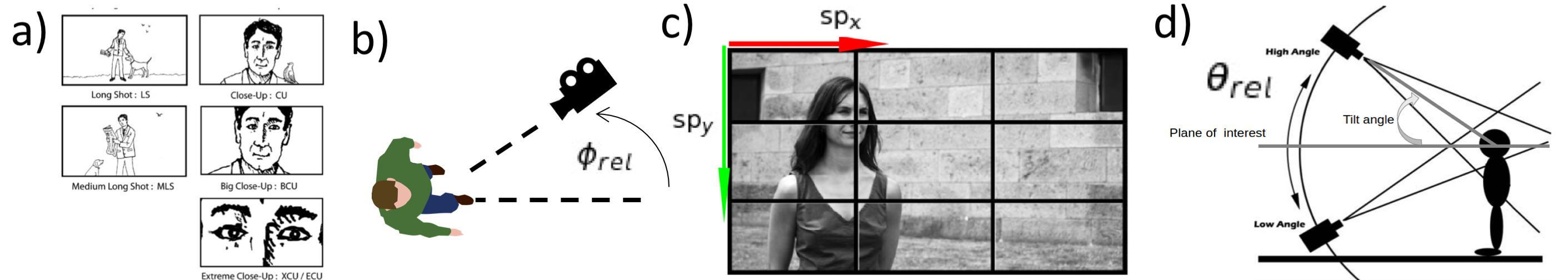
Figure 5: Shot parameters for shot quality cost function, adapted from [11]: a) shot scale $\rho$ corresponds to the size of the projection of the actor on the screen; b) line of action angle $\phi_{rel}\in[0,2\pi]$; c) screen position of the actor projection $sp_{x},sp_{y}\in[0,1]$; d) tilt angle $\theta_{rel}\in[-\pi,\pi]$

Written in a quadratic form, shot quality measures the average squared distance between $\xi_{q}$ and an ideal trajectory $\xi_{shot}$ that only considers positioning via cinematography parameters. $\xi_{shot}$ can be computed analytically: for each point $\xi_{a}(t)$ in the actor motion prediction, the ideal drone position lies on a sphere centered at $\xi_{a}(t)$ with radius $\rho$ defined by the shot scale, relative yaw angle $\phi_{rel}$ and relative tilt angle $\theta_{rel}$ (Fig. 5):

$$\xi_{shot}(t)=\xi_{a}(t)+\rho\begin{bmatrix}cos(\psi_{a}+\phi_{rel})sin(\theta_{rel})\\ sin(\psi_{a}+\phi_{rel})cos(\theta_{rel})\\ cos(\theta_{rel})\end{bmatrix}$$ (3)

$$J_{\mathrm{shot}}\left(\xi_{q},\xi_{a}\right)=\frac{1}{t_{f}}\frac{1}{2}\int_{0}^{t_{f}}||\xi_{q}(t)-\xi_{shot}(\xi_{a}(t))||^{2}dt$$ (4)

$$\approx\frac{1}{2(n-1)}Tr(\xi_{q}^{T}A_{shot}\xi_{q}+2\xi_{q}^{T}b_{shot}+c_{shot})$$

Safety

Given the online map $\mathcal{G}$, we calculate the TSDT $\mathcal{M}:^{3}\to$ as described in Section IV-B. We adopt a cost function from [41] that penalizes proximity to obstacles:

$$c(p)=\begin{cases}-\mathcal{M}(p)+\frac{1}{2}\epsilon_{obs}&\mathcal{M}(p)<0\\ \frac{1}{2\epsilon_{obs}}(\mathcal{M}(p)-\epsilon_{obs})^{2}&0<\mathcal{M}(p)\leq\epsilon_{obs}\\ 0&\text{otherwise}\end{cases}$$ (5)

We can then define the safety cost function [41]:

$$J_{\mathrm{obs}}\left(\xi_{q},\mathcal{M}\right)=\int_{t=0}^{t_{f}}c(\xi(t))\left|\left|\frac{d}{dt}\xi(t)\right|\right|dt$$ (6)

Occlusion avoidance

Even though the concept of occlusion is binary, i.e, we either have or don’t have visibility of the actor, a major contribution of our past work [8] was defining a differentiable cost that expresses a viewpoint’s occlusion intensity among arbitrary obstacle shapes. Mathematically, we define occlusion as the integral of the TSDT cost $c$ over a 2D manifold connecting both trajectories $\xi_{q}$ and $\xi_{a}$. The manifold is built by connecting each drone-actor position pair in time using the path $p(\tau)=\tau\xi_{q}(t)+(1-\tau)\xi_{a}(\xi_{a})$.

$$J_{\mathrm{occ}}\left(\xi_{q},\xi_{a},\mathcal{M}\right)$$ (7)

$$=\int_{t=0}^{t_{f}}\left(\int_{\tau=0}^{1}\;c(p(\tau))\left|\left|\frac{d}{d\tau}p(\tau)\right|\right|d\tau\right)\,\left|\left|\frac{d}{dt}\xi_{q}(t)\right|\right|dt,$$

Our objective is to minimize the total cost function $J\left(\xi_{q}\right)$ (Eq. 1). We do so by covariant gradient descent, using the gradient of the cost function $\nabla J(\xi_{q})$, and an analytic approximation of the Hessian $\nabla^{2}J(\xi_{q})\approx(A_{smooth}+\lambda_{1}A_{shot})$:

$$\xi_{q}^{+}=\xi_{q}-\frac{1}{\eta}(A_{smooth}+\lambda_{1}A_{shot})^{-1}\nabla J(\xi_{q})$$ (8)

This step is repeated till convergence. We follow conventional stopping criteria for descent algorithms, and limit the maximum number of iterations. Note that we only perform the matrix inversion once, outside of the main optimization loop, rendering good convergence rates [8]. We use the current trajectory as initialization for the next planning problem.

V Experiments

V-A Experimental setup

Our platform is a DJI M210 drone, shown in Figure 6. All processing is done with a NVIDIA Jetson TX2, with 8GB of RAM and 6 CPU cores. An independently controlled gimbal DJI Zenmuse X4S records high-resolution images. Our laser sensor is a Velodyne Puck VLP-16 Lite, with $\pm 15^{o}$ vertical field of view and 100m max range.

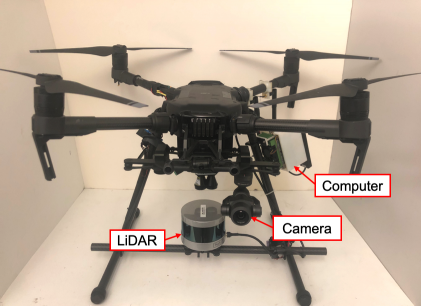
Figure 6: System hardware: DJI M210 drone, Nvidia TX2 computer, VLP16 LiDAR and Zenmuse X4S camera gimbal.

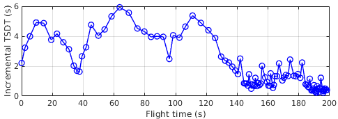
Figure 7: Incremental distance transform compute time over flight time. The first operations take significantly more time because of our map initialization scheme where all cells are initially considered as unknown instead of free. After the first minutes of flight incremental mapping is significantly faster.

V-B Field test results

Visual actor localization

We validate the precision of our pose and heading estimation modules in two experiments where the drone hovers and visually tracks the actor. First, the actor walks between two points over a straight line, and we compare the estimated and ground truth path lengths. Second, the actor walks on a circle at the center of a football field, and we verify the errors in estimated positioning and heading direction. Fig. 8 summarizes our findings.

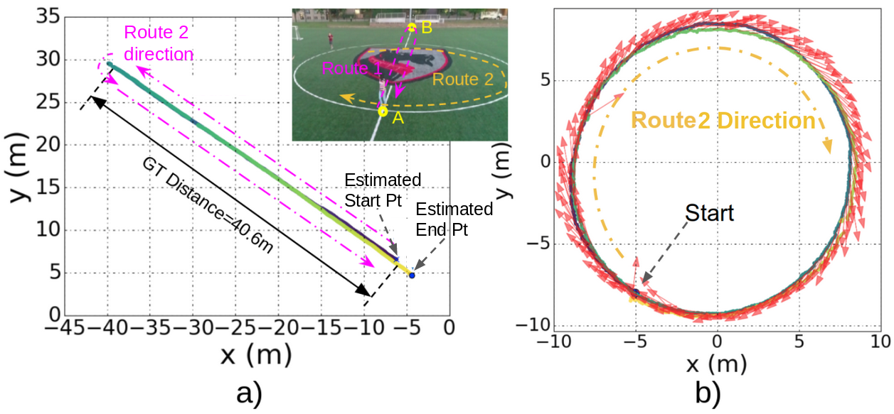
Figure 8: Pose and heading estimation results. a) Actor walks on a straight line from points A-B-A. Ground-truth trajectory length is 40.6m, while the estimated motion length is 42.3m. b) The actor walks along a circle. Ground-truth diameter is 18.3m, while the estimated diameter from ray casting is 18.7m. Heading estimation appears tangential to the ground circle.

Integrated field experiments

We test the real-time performance of our integrated system in several field test experiments. We use our algorithms in unknown and unstructured environments outdoors, following different types of shots and tracking different types of actors (people and bicycles) at both low and high speeds in unscripted scenes. Fig. 9 summarizes the most representative shots, and the supplementary video (https://youtu.be/ZE9MnCVmumc) shows the final footages along with visualizations of point clouds and of the online map.

Figure 9: Field results: a) side shot following biker, b) circling shot around dancer, c) side shot following runner. The UAV trajectory (red) tracks the actor’s forecasted motion (blue), and stays safe while avoiding occlusions from obstacles. We display accumulated point clouds of LiDAR hits and the occupancy grid. Note that LiDAR registration is noisy close to the pole in row (c) due to large electromagnetic interference of wires with the UAV’s compass.

System statistics

We summarize runtime statistics in Table II, and discuss online mapping details in Fig. 7. While the vision networks takes up a large part of the system’s RAM, CPU usage is fairly balanced accross systems.

TABLE II: System statistics

0.2cmSystem	1.0cmModule	2.0cmCPU
	2.0cmRAM (MB)	2.0cmRuntime (ms)
	Detection	57	2160	145
Vision	Tracking	24	25	14.4
	Heading	24	1768	13.9
	KF	8	80	0.207
	Grid	22	48	36.8
Mapping	TSDF	91	810	100-6000
	LiDAR	24	9	NA
Planning	Planner	98	789	198
	DJI SDK	89	40	NA

V-C Performance comparison with full information knowledge

An important hypothesis behind our system is that we can operate with insignificant loss in performance using noisy actor localization and a partially known maps. We compare our system with three assumptions from previous works:

Ground-truth obstacles vs. online map

We compare average planning costs between results from a real-life test where the planner operated while mapping the environment in real time with planning results with the same actor trajectory but with full knowledge of the map beforehand. Results are averaged over 140 s of flight and approximately 700 planning problems. Table III shows a small increase in average planning costs, and Fig 10a shows that qualitatively both trajectories differ minimally. The planning time, however, doubles in the online mapping case due to extra load on CPU.

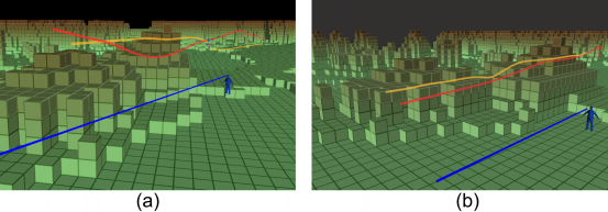
Figure 10: Performance comparisons. a) Planning with full knowledge of the map (yellow) versus with online mapping (red), displayed over ground truth map grid. Online map trajectory is less smooth due to a imperfect LiDAR registration and new obstacle discoveries as flight progresses. b) Planning with perfect ground truth of actor’s location versus noisy actor estimate with artificial noise of 1m amplitude. The planner is able to handle noisy actor localization well due to smoothness cost terms, with final trajectory similar to ground-truth case.

TABLE III: Performance comparisons

2.5cmPlanning Condition	2.5cmAvg. plan
	1.5cmAvg. cost	1.5cmMedian cost
Ground-truth map	32.1	0.1022	0.0603
Online map	69.0	0.1102	0.0825
Ground-truth actor	36.5	0.0539	0.0475
Noise in actor	30.2	0.1276	0.0953

Ground-truth actor versus noisy estimate

We compare the performance between simulated flights where the planner has full knowledge of the actor’s position versus artificially noisy estimates with 1m amplitude. Results are also averaged over 140 s of flight and approximately 700 planning problems, and are displayed on Table III. The large cost difference is due to the shot quality cost, which relies on the actor’s position forecast and is severely penalized by the noise. However, if compared with the actor’s ground-truth trajectory, the difference in cost would be significantly smaller, as seen by the proximity of both final trajectories in Fig 10b. These results offer insight on the importance of our smoothness cost function when handling the noisy visual actor localization.

Height map assumption vs. 3D map

As seen in Fig. 9c, our current system is capable of avoiding unstructured obstacles in 3D environments such as wires and poles. This capability is a significant improvement over our previous work [8], which used a height map assumption.

VI Conclusion

We present a complete system for autonomous aerial cinematography that can localize and track actors in unknown and unstructured environments with onboard computing in real time. Our platform uses a monocular visual input to localize the actor’s position, and a custom-trained network to estimate the actor’s heading direction. Additionally, it maps the world using a LiDAR and incrementally updates a signed distance map. Both of these are used by a camera trajectory planner that produces smooth and artistic trajectories while avoiding obstacles and occlusions. We evaluate the system extensively in different real-world tasks with multiple shot types and varying terrains.

We are actively working on a number of directions based on lessons learned from field trials. Our current approach assumes a static environment. Even though the our mapping can tolerate motion, a principled approach would track moving objects and forecast their motion. The TSDT is expensive to maintain because whenever unknown space is cleared, a large update is computed. We are looking into a just-in-time update that processes only the subset of the map queried by the planner, which is often quite small.

Currently, we do not close the loop between the image captured and the model used by the planner. Identifying model errors, such as actor forecasting or camera calibration, in an online fashion is a challenging next step. The system may also lose the actor due to tracking failures or sudden course changes. An exploration behavior to reacquire the actor is essential for robustness.

ACKNOWLEDGMENT

We thank Mirko Gschwindt, Xiangwei Wang, Greg Armstrong for the assistance in field experiments and robot construction.

References

- [1] N. Joubert, D. B. Goldman, F. Berthouzoz, M. Roberts, J. A. Landay, P. Hanrahan et al., “Towards a drone cinematographer: Guiding quadrotor cameras using visual composition principles,” arXiv preprint arXiv:1610.01691, 2016.
- [2] T. Nägeli, L. Meier, A. Domahidi, J. Alonso-Mora, and O. Hilliges, “Real-time planning for automated multi-view drone cinematography,” ACM Transactions on Graphics (TOG), vol. 36, no. 4, p. 132, 2017.
- [3] Q. Galvane, J. Fleureau, F. L. Tariolle, and P. Guillotel, “Automated cinematography with unmanned aerial vehicles,” in Proceedings of the Eurographics Workshop on Intelligent Cinematography and Editing, 2016.
- [4] Q. Galvane, C. Lino, M. Christie, J. Fleureau, F. Servant, F. Tariolle, P. Guillotel et al., “Directing cinematographic drones,” ACM Transactions on Graphics (TOG), vol. 37, no. 3, p. 34, 2018.
- [5] C. Huang, F. Gao, J. Pan, Z. Yang, W. Qiu, P. Chen, X. Yang, S. Shen, and K.-T. T. Cheng, “Act: An autonomous drone cinematography system for action scenes,” in 2018 IEEE International Conference on Robotics and Automation (ICRA). IEEE, 2018, pp. 7039–7046.
- [6] “Dji mavic,” https://www.dji.com/mavic, accessed: 2019-02-28.
- [7] Skydio. (2018) Skydio R1 self-flying camera. [Online]. Available: https://www.skydio.com/technology/
- [8] R. Bonatti, Y. Zhang, S. Choudhury, W. Wang, and S. Scherer, “Autonomous drone cinematographer: Using artistic principles to create smooth, safe, occlusion-free trajectories for aerial filming,” International Symposium on Experimental Robotics, 2018.
- [9] M. Christie, P. Olivier, and J.-M. Normand, “Camera control in computer graphics,” in Computer Graphics Forum, vol. 27, no. 8. Wiley Online Library, 2008, pp. 2197–2218.
- [10] D. Arijon, “Grammar of the film language,” 1976.
- [11] C. J. Bowen and R. Thompson, Grammar of the Shot. Taylor & Francis, 2013.
- [12] M. Gleicher and A. Witkin, “Through-the-lens camera control,” in ACM SIGGRAPH Computer Graphics, vol. 26, no. 2. ACM, 1992, pp. 331–340.
- [13] S. M. Drucker and D. Zeltzer, “Intelligent camera control in a virtual environment,” in Graphics Interface. Citeseer, 1994, pp. 190–190.
- [14] C. Lino, M. Christie, R. Ranon, and W. Bares, “The director’s lens: an intelligent assistant for virtual cinematography,” in Proceedings of the 19th ACM international conference on Multimedia. ACM, 2011, pp. 323–332.
- [15] C. Lino and M. Christie, “Intuitive and efficient camera control with the toric space,” ACM Transactions on Graphics (TOG), vol. 34, no. 4, p. 82, 2015.
- [16] M. Roberts and P. Hanrahan, “Generating dynamically feasible trajectories for quadrotor cameras,” ACM Transactions on Graphics (TOG), vol. 35, no. 4, p. 61, 2016.
- [17] N. Joubert, M. Roberts, A. Truong, F. Berthouzoz, and P. Hanrahan, “An interactive tool for designing quadrotor camera shots,” ACM Transactions on Graphics (TOG), vol. 34, no. 6, p. 238, 2015.
- [18] C. Gebhardt, S. Stevsic, and O. Hilliges, “Optimizing for aesthetically pleasing quadrotor camera motion,” 2018.
- [19] C. Gebhardt, B. Hepp, T. Nägeli, S. Stevšić, and O. Hilliges, “Airways: Optimization-based planning of quadrotor trajectories according to high-level user goals,” in Proceedings of the 2016 CHI Conference on Human Factors in Computing Systems. ACM, 2016, pp. 2508–2519.
- [20] K. Xie, H. Yang, S. Huang, D. Lischinski, M. Christie, K. Xu, M. Gong, D. Cohen-Or, and H. Huang, “Creating and chaining camera moves for quadrotor videography,” ACM Transactions on Graphics, vol. 37, p. 14, 2018.
- [21] Z. Lan, M. Shridhar, D. Hsu, and S. Zhao, “Xpose: Reinventing user interaction with flying cameras,” in Robotics: Science and Systems, 2017.
- [22] C. Huang, Z. Yang, Y. Kong, P. Chen, X. Yang, and K.-T. T. Cheng, “Through-the-lens drone filming,” in 2018 IEEE/RSJ International Conference on Intelligent Robots and Systems (IROS). IEEE, 2018, pp. 4692–4699.
- [23] S. Thrun, W. Burgard, and D. Fox, Probabilistic robotics. MIT press, 2005.
- [24] S. Isler, R. Sabzevari, J. Delmerico, and D. Scaramuzza, “An information gain formulation for active volumetric 3d reconstruction,” in ICRA, 2016.
- [25] B. Charrow, G. Kahn, S. Patil, S. Liu, K. Goldberg, P. Abbeel, N. Michael, and V. Kumar, “Information-theoretic planning with trajectory optimization for dense 3d mapping,” in RSS, 2015.
- [26] R. A. Newcombe, S. Izadi, O. Hilliges, D. Molyneaux, D. Kim, A. J. Davison, P. Kohi, J. Shotton, S. Hodges, and A. Fitzgibbon, “Kinectfusion: Real-time dense surface mapping and tracking,” in Mixed and augmented reality (ISMAR), 2011 10th IEEE international symposium on. IEEE, 2011, pp. 127–136.
- [27] M. Klingensmith, I. Dryanovski, S. Srinivasa, and J. Xiao, “Chisel: Real time large scale 3d reconstruction onboard a mobile device using spatially hashed signed distance fields.” in Robotics: Science and Systems, vol. 4, 2015.
- [28] H. Oleynikova, Z. Taylor, M. Fehr, J. Nieto, and R. Siegwart, “Voxblox: Incremental 3d euclidean signed distance fields for on-board mav planning,” arXiv preprint arXiv:1611.03631, 2016.
- [29] H. Cover, S. Choudhury, S. Scherer, and S. Singh, “Sparse tangential network (spartan): Motion planning for micro aerial vehicles,” in 2013 IEEE International Conference on Robotics and Automation. IEEE, 2013, pp. 2820–2825.
- [30] J. Redmon and A. Farhadi, “Yolov3: An incremental improvement,” CoRR, vol. abs/1804.02767, 2018. [Online]. Available: http://arxiv.org/abs/1804.02767
- [31] S. Ren, K. He, R. B. Girshick, and J. Sun, “Faster R-CNN: towards real-time object detection with region proposal networks,” CoRR, vol. abs/1506.01497, 2015. [Online]. Available: http://arxiv.org/abs/1506.01497
- [32] M. Raza, Z. Chen, S.-U. Rehman, P. Wang, and P. Bao, “Appearance based pedestrians’ head pose and body orientation estimation using deep learning,” Neurocomputing, vol. 272, pp. 647–659, 2018.
- [33] S. Li and A. Chan, “3d human pose estimation from monocular images with deep convolutional neural network,” vol. 9004, 11 2014, pp. 332–347.
- [34] A. G. Howard, M. Zhu, B. Chen, D. Kalenichenko, W. Wang, T. Weyand, M. Andreetto, and H. Adam, “Mobilenets: Efficient convolutional neural networks for mobile vision applications,” arXiv preprint arXiv:1704.04861, 2017.
- [35] X. Zhang, X. Zhou, M. Lin, and J. Sun, “Shufflenet: An extremely efficient convolutional neural network for mobile devices,” in The IEEE Conference on Computer Vision and Pattern Recognition (CVPR), June 2018.
- [36] W. Wang, A. Ahuja, Y. Zhang, R. Bonatti, and S. Scherer, “Improved generalization of heading direction estimation for aerial filming using semi-supervised regression,” Robotics and Automation (ICRA), 2019 IEEE International Conference on, 2019.
- [37] T.-Y. Lin, M. Maire, S. Belongie, J. Hays, P. Perona, D. Ramanan, P. Dollár, and C. L. Zitnick, “Microsoft coco: Common objects in context,” in European conference on computer vision. Springer, 2014, pp. 740–755.
- [38] J. F. Henriques, R. Caseiro, P. Martins, and J. Batista, “High-speed tracking with kernelized correlation filters,” IEEE Transactions on Pattern Analysis and Machine Intelligence, vol. 37, no. 3, pp. 583–596, 2015.
- [39] A. Toshev and C. Szegedy, “Deeppose: Human pose estimation via deep neural networks,” in Proceedings of the IEEE conference on computer vision and pattern recognition, 2014, pp. 1653–1660.
- [40] Z. Cao, T. Simon, S.-E. Wei, and Y. Sheikh, “Realtime multi-person 2d pose estimation using part affinity fields,” in CVPR, 2017.
- [41] M. Zucker, N. Ratliff, A. D. Dragan, M. Pivtoraiko, M. Klingensmith, C. M. Dellin, J. A. Bagnell, and S. S. Srinivasa, “CHOMP: Covariant hamiltonian optimization for motion planning,” The International Journal of Robotics Research, vol. 32, no. 9-10, pp. 1164–1193, 2013.