Constraining extra gravitational wave polarizations with Advanced LIGO, Advanced Virgo and KAGRA and upper bounds from GW170817

Abstract

General metric theories of gravity in four-dimensional spacetimes can contain at most six polarization modes (two spin-0, two spin-1 and two spin-2) of gravitational waves (GWs). It has been recently shown that, with using four GW non-coaligned detectors, a direct test of the spin-1 modes can be done in principle separately from the spin-0 and spin-2 modes for a GW source in particular sky positions [Hagihara et al., Phys. Rev. D 98, 064035 (2018)]. They have found particular sky positions that satisfy a condition of killing completely the spin-0 modes in a so-called null stream which is a linear combination of the signal outputs to kill the spin-2 modes. The present paper expands the method to discuss a possibility that the spin-0 modes are not completely but effectively suppressed in the null streams to test the spin-1 modes separately from the other modes, especially with an expected network of Advanced LIGO, Advanced Virgo and KAGRA. We study also a possibility that the spin-1 modes are substantially suppressed in the null streams to test the spin-0 modes separately from the other modes, though the spin-1 modes for any sky position cannot be completely killed in the null streams. Moreover, we find that the coefficient of the spin-0 modes in the null stream is significantly small for the GW170817 event, so that an upper bound can be placed on the amplitude of the spin-1 modes as $<6\times 10^{-23}$.

I Introduction

Gravitational waves (GWs) in Einstein’s theory of general relativity (GR), spacetime ripples that propagate at the speed of light, can be formulated in terms of the so-called “tensor” modes which are spin-2 transverse and traceless (TT) parts of the spacetime metric Einstein1916 ; Einstein1918 . The speed of the GW propagation has been confirmed surprisingly at the level of $\sim O(10^{-15})$ by the GW170817 event with an electromagnetic (EM) counterpart as the first observation of GWs from a NS-NS merger GW170817 . In the rest of the present paper, we assume that the speed of GWs is almost the same as the speed of light. For a GW source with an EM counterpart, we know its precise location on the sky. In the present paper, we use essentially the information mainly on the direction of the GW source. Note that the assumption on the GW speed is not crucial in the present method. Extra GW modes may be delayed. For a few seconds (or minutes) delay, we will be able to still recognize that the delayed signals come from the same GW source and thus the sky location of the GW source is known from EM observations.

Alternative theories to GR, more specifically general metric theories of gravity in four-dimensional spacetimes can predict extra degrees of freedom with spin 0 and spin 1, which are usually called scalar and vector modes, respectively Eardley ; PW . Future detection of scalar or vector GW polarization would provide serious evidence against GR. Or future GW polarization tests would place a strong constraint on scalar and vector modes of GWs, which will lead to a new test of modified gravity theories, some of which might be ruled out. Therefore, many attempts for GW polarization tests by using not only bursts, pulsars, compact binary coalescences, but also stochastic sources have been discussed (e.g. Isi2015 ; Isi2017 ; Svidzinsky ; pulsar ; Nishizawa2009 ; Hayama ; Nishizawa2018 ).

The GW astronomy has just started and aLIGO-Hanford (H), aLIGO-Livingston (L) and Virgo (V) have already detected GW signals. HLV will start the O3 observation run in April this year. However, three detectors are not enough for distinguishing every polarization of GWs. The construction of another kilometer-scale interferometer called KAGRA (K) is currently urged to join the GW detector network as a fourth detector by the end of the O3 run. See Reference LVK for a comprehensive review on the expected network of Advanced LIGO, Advanced Virgo and KAGRA (denoted as HLVK). Therefore, it is currently interesting to examine how to probe extra GW polarizations by HLVK.

It was thought that five or more non-coaligned GW interferometers were needed to directly test the extra degrees of freedom of GW with spin 0 and 1 separately from each other. In fact, Chatziioannou, Yunes and Cornish have argued null streams for six (or more) GW detectors to probe GW polarizations CYC . The null stream approach was introduced first by Gürsel and Tinto GT and was extended by Wen and Schutz WS and Chatterji et al. null-papers , where the idea behind the null stream method is that there exists a linear combination of the data from a network of detectors, such that the linear combination called a null stream can contain no tensor modes but only noise in GR cases. Gürsel and Tinto GT proposed the use of the null stream in order to understand the noise behavior.

Assuming that, for a given source of GWs, its sky position is known, as is the case of GW events with an electromagnetic (EM) counterpart such as GW170817, however, it has been recently found that there are particular sky positions that satisfy a condition for the spin-0 modes to be killed completely in the null streams in which the spin-2 GW modes disappear and thus the spin-1 modes can be directly tested separately from the spin-0 and spin-2 modes, even with using only four GW non-coaligned detectors, though the strain output at a detector may contain the spin-0 modes Hagihara . They have found that there are seventy sky positions exactly at which the spin-0 modes are killed in the null streams.

However, the area of the seventy points is zero. Does this mean that the probability of such a potentially important event is negligible? In order to answer this, we shall examine whether a GW source near one of the seventy sky positions can be used for testing (e.g. placing an upper bound on) spin-1 GW modes, if the spin-0 modes are substantially suppressed even though they are not perfectly killed.

How large is the sky area where the spin-0 modes are significantly suppressed and thus the spin-1 modes can be tested separately from the other modes? This is an interesting subject, especially for the near future GW observations with using the HLVK network.

The main purpose of this paper is to examine how large is the probability that spin-0 modes are substantially suppressed and thus spin-1 GW modes can be tested separately from the other GW polarizations by HLVK. This paper is organized as follows. In Section II, we describe null streams for four non-coaligned detectors. In Section III, we discuss a possibility that the spin-0 modes are substantially suppressed in the null streams and hence the spin-1 modes can be tested within the noise level, especially with an expected network of HLVK. In Section IV, we study also a possibility that the spin-1 modes are almost killed in the null streams and thus the spin-0 modes become testable separately from the other modes. In Section V, we discuss a constraint on the spin-1 modes by the GW170817 event. Section VI is devoted to a summary of this paper. Throughout this paper, Latin indices $a,b,\cdots$ run from 1 to 4 corresponding to four detectors.

II Null streams for four non-coaligned detectors

Let us assume that there exist four non-coaligned detectors with uncorrelated noise. Each detector is labeled by $a$ ($a=1,2,3$ and $4$). We assume also that, for a given GW source, we know its sky position, as is the case of GW events with an EM counterpart such as GW170817. By the second assumption, we know exactly how to shift the arrival time of the GW from detector to detector.

For each detector, the signal from a GW source at the sky location denoted as $(\theta,\phi)$ is written as

$$S_{a}= F_{a}^{+}h_{+}+F_{a}^{\times}h_{\times}$$

$$+F_{a}^{S}h_{S}+F_{a}^{L}h_{L}$$

$$+F_{a}^{V}h_{V}+F_{a}^{W}h_{W}+n_{a},$$ (1)

where $h_{+}$ and $h_{\times}$ denote the spin-2 modes called the plus and cross mode, respectively, $h_{S}$ and $h_{L}$ denote the spin-0 modes called the breathing and longitudinal mode, respectively, and $h_{V}$ and $h_{W}$ denote the spin-1 modes often called the vector-$x$ and vector-$y$ mode, respectively footnote0 , $F_{a}^{+}$, $F_{a}^{\times}$, $F_{a}^{S}$, $F_{a}^{L}$, $F_{a}^{V}$ and $F_{a}^{W}$ are the antenna patterns for GW polarizations PW ; Nishizawa2009 ; ST and $n_{a}$ denotes noise at the detector. The antenna patterns are functions of a GW source location $\theta$ and $\phi$ footnote1 . In our numerical calculations, $\theta$ and $\phi$ denote the latitude and longitude, respectively.

By noting $F_{a}^{S}=-F_{a}^{L}$ footnote2 that was shown by Nishizawa et al. in Nishizawa2009 , Eq. (1) can be simplified as

$$S_{a}= F_{a}^{+}h_{+}+F_{a}^{\times}h_{\times}$$

$$+F_{a}^{S}(h_{S}-h_{L})$$

$$+F_{a}^{V}h_{V}+F_{a}^{W}h_{W}+n_{a}.$$ (2)

Note that the effects of $h_{S}$ on the detector are exactly the same with the opposite sign as those of $h_{L}$. Hence, GW interferometers can test only the difference as $h_{S}-h_{L}$, one combined spin-0 mode.

Eq. (2) may suggest that five or more non-coaligned detectors are needed for measuring five components $h_{+}$, $h_{\times}$, $h_{V}$, $h_{W}$ and $h_{S}-h_{L}$. This is related with the inversion of a $5\times 5$ matrix. Namely, the existence of the inverse matrix is assumed implicitly when the above suggestion holds. In fact, Hagihara et al. have found that there are exceptional cases, for which spin-0 modes are completely killed and thus spin-1 modes can be tested separately from spin-2 and spin-0 modes. Their study is entirely based on the null streams. The null stream was introduced first by Gürsel and Tinto GT , who considered only the purely tensorial modes $h_{\times}$ and $h_{+}$. Let us imagine, for its simplicity, an ideal case that noise is negligible in Eq. (2). Then, by straightforward calculations, one can obtain a null stream GT as, for three detectors as $a=1,2$ and $3$ for instance,

$$\delta_{23}S_{1}+\delta_{31}S_{2}+\delta_{12}S_{3}=0,$$ (3)

where we define

$$\delta_{ab}\equiv F_{a}^{+}F_{b}^{\times}-F_{b}^{+}F_{a}^{\times}.$$ (4)

Namely, signal outputs at the three detectors must satisfy Eq. (3), provided that the signals are made only from the spin-2 waves.

For four GW detectors with noise, the null streams become

$$\delta_{23}S_{1}+\delta_{31}S_{2}+\delta_{12}S_{3} =\delta_{23}n_{1}+\delta_{31}n_{2}+\delta_{12}n_{3},$$ (5)

$$\delta_{34}S_{2}+\delta_{42}S_{3}+\delta_{23}S_{4} =\delta_{34}n_{2}+\delta_{42}n_{3}+\delta_{23}n_{4},$$ (6)

$$\delta_{41}S_{3}+\delta_{13}S_{4}+\delta_{34}S_{1} =\delta_{41}n_{3}+\delta_{13}n_{4}+\delta_{34}n_{1},$$ (7)

$$\delta_{12}S_{4}+\delta_{24}S_{1}+\delta_{41}S_{2} =\delta_{12}n_{4}+\delta_{24}n_{1}+\delta_{41}n_{2}.$$ (8)

The number of independent equations in Eqs. (5)-(8) is two Hagihara .

Next, we incorporate scalar and vector polarization modes. Only the tensor modes cancel out in the tensor null stream as Eq. (2). The scalar and vector modes can exist in the null stream. Two null streams can be written as Hagihara

$$P_{a}S_{a} =(P_{b}F_{b}^{S})(h_{S}-h_{L})+(P_{c}F_{c}^{V})h_{V}+(P_{d}F_{d}^{W})h_{W}+P_{e}n_{e},$$ (9)

$$Q_{f}S_{f} =(Q_{g}F_{g}^{S})(h_{S}-h_{L})+(Q_{h}F_{h}^{V})h_{V}+(Q_{i}F_{i}^{W})h_{W}+Q_{j}n_{j},$$ (10)

where we use Eq. (2) and the summation is taken over $a,\cdots,j=1,2,3$ and $4$. Note that the tensor null stream is built in and hence $h_{+}$ and $h_{\times}$ do not appear in the above equations. Without loss of generality, we can choose $P_{a}$ and $Q_{a}$ as $(P_{a})=(\delta_{23},\delta_{31},\delta_{12},0)$ and $(Q_{a})=(0,\delta_{34},\delta_{42},\delta_{23})$ for its simplicity, which are corresponding to Eqs. (5) and (6) in the previous paragraph.

In the following sections, we shall examine Eqs. (9) and (10) in more detail. In numerical calculations for the HLVK network, we choose H=1, L=2, V=3 and K=4 for $a=1,2,3$ and $4$ for its simplicity.

III Suppression of spin-0 modes

Let us study the behavior of the spin-0 modes in the null streams by Eqs. (9) and (10), in which the coefficients of $h_{S}-h_{L}$ are $P_{a}F_{a}^{S}$ and $Q_{a}F_{a}^{S}$, respectively. Note that the tensor null stream is built in and hence $h_{+}$ and $h_{\times}$ do not exist in the equations.

If $P_{a}F_{a}^{S}$ and $Q_{a}F_{a}^{S}$ are substantially small, spin-0 GW components can be taken to make a small contribution to the null streams. We look for quantitative criteria about whether or not the coefficients are small. In this paper, we do not assume a particular model of modified gravity. As a candidate for such criteria, therefore, we define a suppression factor by

$$\rho^{S}\equiv\frac{\max(|\mbox{PQF}^{S}|)-|\mbox{PQF}^{S}|}{\max(|\mbox{PQF}^{S}|)},$$ (11)

where $|\mbox{PQF}^{S}|$ denotes that larger one of $|P_{a}F_{a}^{S}|$ and $|Q_{a}F_{a}^{S}|$ and $\max(|\mbox{PQF}^{S}|)$ is the largest one of $|\mbox{PQF}^{S}|$ for the observed events. This approach is a possible extension of Reference Hagihara , in which they focused only on the sky positions corresponding to $\rho^{S}=1$. In realistic situations, each detector has noise and thus $\rho^{S}=1$ is too strict. Therefore, introducing the suppression factor in the discussion will make the present approach more practical for use.

Figure 1 shows the sky map, which is the contour map for the coefficients of the scalar modes in the null streams by Eqs. (9) and (10). At some positions in the contour map, one can recognize an octapolar behavior of some curves. This behavior is because $\delta_{ab}$ is quadratic in $F_{a}^{+}$ and $F_{b}^{\times}$, where the GW antenna pattern functions are quadratic in trigonometric functions of $\theta$ and $\phi$. This figure shows that GW source positions with the suppression factor $\rho^{S}\geq 0.9$ have a significantly large area in the whole sky. We should note that domains with a much larger suppression factor $\rho^{S}\geq 0.99$ can be still recognized by eyes in the contour map. The probability for such largely suppressed events is not so negligible.

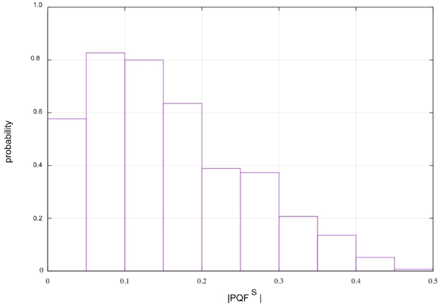
Figure 2: The vertical axis denotes the probability for each bin, where the horizontal axis denotes $|\mbox{PQF}^{S}|$, namely the larger one of $|P_{a}F_{a}^{S}|$ and $|Q_{a}F_{a}^{S}|$ in the null stream. We prepare numerically a random distribution of 10,000 events in the sky. The probability distribution has a single peak around $\sim 0.1$. The overall behavior of this histogram is confirmed numerically by changing the total number of events such as 20,000 and 100,000.

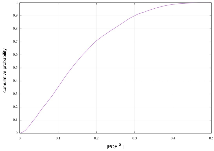
Figure 3: Event rate v.s. the threshold on $|\mbox{PQF}^{S}|$, the larger one of $|P_{a}F_{a}^{S}|$ and $|Q_{a}F_{a}^{S}|$ for the scalar mode, corresponding to Figure 2. The cumulative probability in the vertical axis increases as the threshold for the suppression factor becomes larger.

We discuss the probability distribution of the coefficient $|\mbox{PQF}^{S}|$ in the null streams by numerically generating 10,000 GW events randomly located on the sky. Figure 2 shows the probability distribution as a function of the larger one between the two coefficients. The statistical fluctuation in each bin of the histogram is small ($\sim$ a few percents), so that overall it cannot affect the shape of the histogram. This figure suggests that events with a large suppression factor may have a substantial probability. For this to be clearer, we plot the cumulative probability distribution of events. See figure 3. If we choose the threshold for the suppression factor on the scalar modes as $\rho^{S}\geq 0.8$ (corresponding to $|\mbox{PQF}^{S}|\leq 0.1$) for instance, then, nearly 30 percents of the total events can be used for a practical test of spin-1 polarizations. Even if we choose a tighter threshold as $\rho^{S}\geq 0.9$ (corresponding to $|\mbox{PQF}^{S}|\leq 0.05$), nearly 20 percents of the events can be still used for a separate test of spin-1 modes. Roughly speaking, if five GW events with EM counterparts are detected in future, one of the events can be used for spin-1 tests.

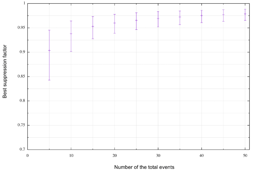
Figure 4: The vertical axis denotes the best suppression factor that is expected for a given total event number which is denoted as the horizontal axis. The error bars represent $1\sigma$ deviation. If the number of observed events is increased up to ten for example, the best suppression may reach 0.9 or more. For this case, a contribution of the scalar modes in the null streams is suppressed by a factor of ten or more and hence such an event can be practically used for a separate test of the spin-1 modes.

Figure 4 shows the best suppression factor that can be expected for a given number of the total events. If about ten events are observed, the best suppression is likely to be 0.9 more or less, so that such an event with a large suppression can be used as a probe of the vector GW mode.

IV Suppression of spin-1 modes

Next, we consider a suppression of the spin-1 modes in the null stream. This subject is new in the sense that Reference Hagihara does not study the suppression of the spin-1 modes. First, we examine whether or not $P_{a}F_{a}^{V}$, $P_{a}F_{a}^{W}$, $Q_{a}F_{a}^{V}$ and $Q_{a}F_{a}^{W}$ vanish simultaneously at a sky position for the HLVK network. Our numerical result shows that they never do. This is a marked contrast to the spin-0 case, for which the two scalar coefficients $P_{a}F_{a}^{S}$ and $Q_{a}F_{a}^{S}$ can simultaneously vanish (and actually do at seventy positions in the sky Hagihara ). This can be understood by noting that two curves on a surface can intersect at some point, if they are not lines parallel to each other. On the other hand, three (or more) curves do not generally pass through the same point except for very special cases.

For the practical purpose, however, if all of $P_{a}F_{a}^{V}$, $P_{a}F_{a}^{W}$, $Q_{a}F_{a}^{V}$ and $Q_{a}F_{a}^{W}$ are small in the neighborhood of a certain sky location, a contribution of the spin-1 modes to the right-hand sides of the null streams is so small that such a case can give us an opportunity for a test of spin-0 polarizations. Therefore, let us examine how often the simultaneous suppression of the four vector coefficients in Eqs. (9) and (10) can occur.

First, we should note that $P_{a}F_{a}^{V}$ and $P_{a}F_{a}^{W}$ are related with each other, because of the spin-1 nature. One can show that $(P_{a}F_{a}^{V})^{2}+(P_{a}F_{a}^{W})^{2}$ is invariant for the spatial rotation around the axis of the GW propagation direction as follows.

Let us consider a rotation around the GW propagation axis with the rotation angle denoted as $\psi$. The GW spin-1 modes are transformed as

$$\left(\begin{array}[]{c}h_{V}^{\prime}\\ h_{W}^{\prime}\end{array}\right) =\left(\begin{array}[]{cc}\cos\psi&-\sin\psi\\ \sin\psi&\cos\psi\end{array}\right)\left(\begin{array}[]{c}h_{V}\\ h_{W}\end{array}\right),$$ (18)

where the prime denotes the rotation with $\psi$. In Eq. (9), the left-hand side including the detectors’ signals do nothing to do with the above rotation with $\psi$. The first term and the last one of the right-hand side in Eq. (9) are spin-0 and the detectors’ noise, respectively, and thus they are independent of the $\psi$ rotation. As a result, the sum of the remaining (second and third) terms of the right-hand side is independent of the $\psi$ rotation, though each term may change by the rotation. Namely, we find for any $h_{V}$ and $h_{W}$

$$(P_{a}^{\prime}F_{a}^{V\prime})h_{V}^{\prime}+(P_{a}^{\prime}F_{a}^{W\prime})h_{W}^{\prime}=(P_{a}F_{a}^{V})h_{V}+(P_{a}F_{a}^{W})h_{W}.$$ (19)

By using Eq. (18) for Eq. (19), we obtain

$$\left(\begin{array}[]{c}P_{a}^{\prime}F_{a}^{V\prime}\\ P_{a}^{\prime}F_{a}^{W\prime}\end{array}\right) =\left(\begin{array}[]{cc}\cos\psi&-\sin\psi\\ \sin\psi&\cos\psi\end{array}\right)\left(\begin{array}[]{c}P_{a}F_{a}^{V}\\ P_{a}F_{a}^{W}\end{array}\right).$$ (26)

This means that $(P_{a}F_{a}^{V},P_{a}F_{a}^{W})$ is a spin-1 vector. This spin-1 property can be shown also by straightforward calculations of using explicit forms of $P_{a}$, $F_{a}^{V}$ and $F_{a}^{W}$. From Eq. (26), one can immediately show that the squared magnitude as $(P_{a}F_{a}^{V})^{2}+(P_{a}F_{a}^{W})^{2}$ remains unchanged by the rotation.

Hence, we use the invariant combination

$$PF^{VW} \equiv\sqrt{(P_{a}F_{a}^{V})^{2}+(P_{a}F_{a}^{W})^{2}},$$ (27)

$$QF^{VW} \equiv\sqrt{(Q_{a}F_{a}^{V})^{2}+(Q_{a}F_{a}^{W})^{2}},$$ (28)

to define, by the same way for Eq. (11), the suppression factor for the vector modes as

$$\rho^{VW}\equiv\frac{\max(\mbox{PQF}^{VW})-\mbox{PQF}^{VW}}{\max(\mbox{PQF}^{VW})},$$ (29)

where $\mbox{PQF}^{VW}$ denotes that larger one of $PF^{VW}$ and $QF^{VW}$ and $\max(\mbox{PQF}^{VW})$ is the largest one of $\mbox{PQF}^{VW}$ for the observed events. Here, the magnitude of $(P_{a}F_{a}^{V},P_{a}F_{a}^{W})$ is corresponding to the scalar counterpart as $P_{a}F_{a}^{S}$.

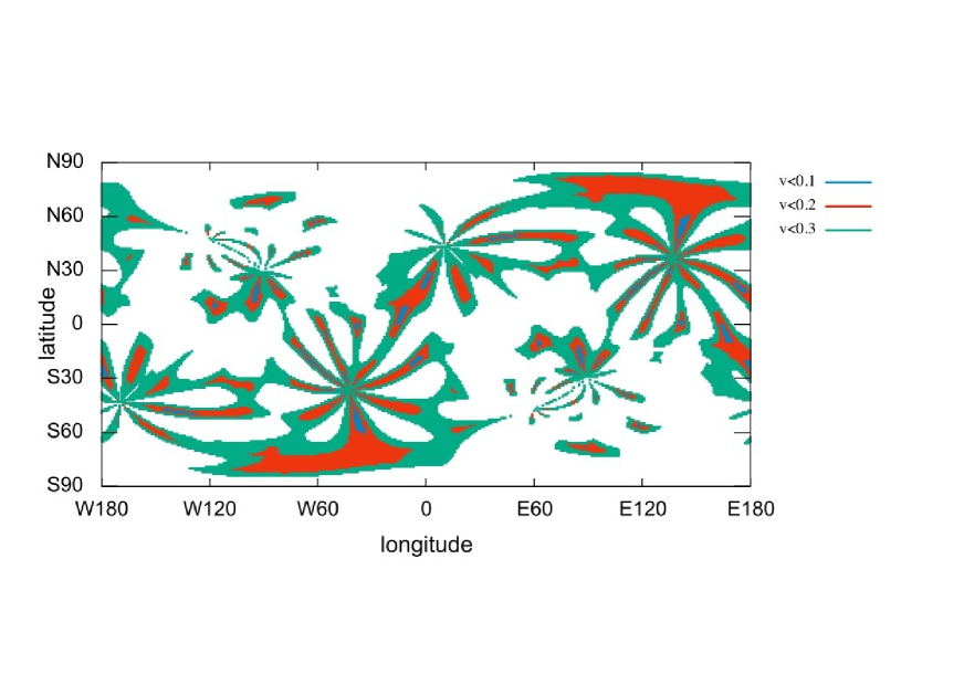
Figure 5: Contour map of $\mbox{PQF}^{VW}$, namely the larger one between $\sqrt{(P_{a}F_{a}^{V})^{2}+(P_{a}F_{a}^{W})^{2}}$ and $\sqrt{(Q_{a}F_{a}^{V})^{2}+(Q_{a}F_{a}^{W})^{2}}$ in the null stream for the HLVK network. The vertical and horizontal axes denote the latitude and longitude of a GW source, respectively. The maximum value of each of the vector coefficients is unity.

Figure 5 is the contour map for $\sqrt{(P_{a}F_{a}^{V})^{2}+(P_{a}F_{a}^{W})^{2}}$. This figure shows that GW events with the suppression factor $\rho^{VW}\geq 0.9$ occur in nearly one percent of the whole sky area. This figure implies that the suppression of the vector modes occurs less frequently than that of the scalar modes. For instance, the area of the suppression of the vector modes as $\rho^{VW}\geq 0.9$ is much smaller than that for the scalar modes as $\rho^{S}\geq 0.9$. This contrast comes from the difference in the number of the related coefficients in the null streams: The coefficient for the scalar is $P_{a}F_{a}^{S}$ in Eq. (9), while those for the vector modes are $P_{a}F_{a}^{V}$ and $P_{a}F_{a}^{W}$. As a result, the probability that both $P_{a}F_{a}^{V}$ and $P_{a}F_{a}^{W}$ are simultaneously small enough to achieve a large $\rho^{VW}$ is small.

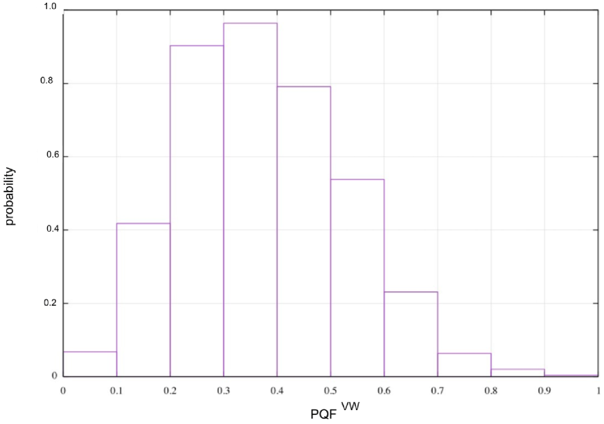
Figure 6: The vertical axis denotes the probability for each bin, where the horizontal axis denotes the largest vector coefficient in the null streams. We prepare numerically a random distribution of 10,000 events in the sky. The probability distribution has a single peak around $\sim 0.3$. The overall behavior of this histogram is confirmed numerically by changing the total number of events such as 20,000 and 100,000.

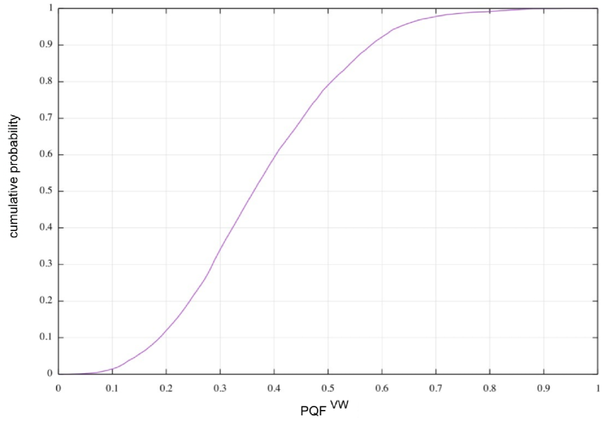
Figure 7: Event probability v.s. the threshold of the suppression factor for the vector mode. The cumulative probability in the vertical axis increases as the threshold for the suppression factor is larger.

Figure 6 is a histogram of GW events for a random distribution of GW sources in the sky, where the horizontal axis denotes the larger one of $\sqrt{(P_{a}F_{a}^{V})^{2}+(P_{a}F_{a}^{W})^{2}}$ and $\sqrt{(Q_{a}F_{a}^{V})^{2}+(Q_{a}F_{a}^{W})^{2}}$. In Figure 6 , there is an excess around $0.2\sim 0.5$. Therefore, we can expect that the probability of testing the spin-0 modes with suppressing the vector modes is not low. We plot also the cumulative probability distribution of events. See figure 7. If we choose the threshold for the suppression factor $\rho^{VW}$ on the vector modes as $\rho^{VW}\geq 0.8$ (corresponding to $\mbox{PQF}^{VW}\leq 0.2$) for instance, then, nearly one of ten events can be used for a practical test of spin-0 polarizations. If we choose a tighter threshold as $\rho^{VW}\geq 0.9$ (corresponding to $\mbox{PQF}^{VW}\leq 0.1$), only 2 percents of the events can be used for a separate test of spin-0 modes. Roughly speaking, the event rate for the suppression of vector modes is smaller by a factor of nearly five than that of the scalar suppression, as shown by Figures 3 and 7.

V GW170817

In this section, we mention GW170817 event GW170817 . For this event, HKV made observations, while KAGRA was under construction. Hence, the null stream for $P_{a}$ can be used for real data analysis of GW170817, while that for $Q_{a}$ will be used only for a theoretical interest but not for any real data analysis. The coefficients in the null streams are estimated as $P_{a}F_{a}^{S}=-0.0738$, $P_{a}F_{a}^{V}=0.3772$, $P_{a}F_{a}^{W}=0.3245$, $Q_{a}F_{a}^{S}=0.0091$, $Q_{a}F_{a}^{V}=0.2924$, $Q_{a}F_{a}^{W}=0.3768$, where the reference for polarization angles is chosen as aLIGO-Livingston ($a=2$). Therefore, $\sqrt{(P_{a}F_{a}^{V})^{2}+(P_{a}F_{a}^{W})^{2}}=0.4976$, and $\sqrt{(Q_{a}F_{a}^{V})^{2}+(Q_{a}F_{a}^{W})^{2}}=0.4769$. Interestingly, the sky position of GW170817 is very particular, in the sense that the scalar coefficient $P_{a}F_{a}^{S}$ for the HLV network is significantly small. If $|P_{a}|$ is small, however, not only $P_{a}F_{a}^{S}$ but also $P_{a}F_{a}^{V}$ and $P_{a}F_{a}^{W}$ are small. For such a case, one cannot test separately the scalar and vector modes. If the coefficients in the null streams are normalized by the magnitude of $P_{a}$ or $Q_{a}$ in order to exclude the case of small $|P_{a}|$ or $|Q_{a}|$, they are $P_{a}F_{a}^{S}/|P_{a}|=-0.1540$, $P_{a}F_{a}^{V}/|P_{a}|=0.7868$, $P_{a}F_{a}^{W}/|P_{a}|=0.6768$, $Q_{a}F_{a}^{S}/|Q_{a}|=0.0212$, $Q_{a}F_{a}^{V}/|Q_{a}|=0.6853$, $Q_{a}F_{a}^{W}/|Q_{a}|=0.8831$, $\sqrt{(P_{a}F_{a}^{V})^{2}+(P_{a}F_{a}^{W})^{2}}/|P_{a}|=1.037$, and $\sqrt{(Q_{a}F_{a}^{V})^{2}+(Q_{a}F_{a}^{W})^{2}}/|Q_{a}|=1.118$. The scalar coefficients are thus much smaller than the vector ones, even after they are normalized.

Figure 9 shows the null stream for $P_{a}$ of the three detector outputs GW170817-data for GW170817. We examine the GW data in the time domain from $-15$ to $+15$ seconds around the GW170817 event, for which the velocity of the vector GWs (denoted as $c_{g}^{\mbox{vect}}$) is limited within

$$\left|\frac{c_{g}^{\mbox{vect}}-c}{c}\right|\leq 4\times 10^{-15}\left(\frac{40\mbox{Mpc}}{D}\right)\left(\frac{|\delta t|}{15\mbox{sec.}}\right),$$ (30)

where $D$ is the distance to the GW source and $\delta t$ is the arrival time difference between the spin-2 and spin-1 waves. In this figure, there are no chirp-like signals around the GW arrival time. This is consistent with that spin-2 modes cancel out in the null stream. Roughly speaking, $|P_{a}S_{a}|<2\times 10^{-23}$ in Figure 9. Therefore, an upper bound on the vector GWs can be placed as $|h^{V}+h^{W}|<6\times 10^{-23}$, where we use an approximation as $P_{a}F_{a}^{V}\sim P_{a}F_{a}^{W}\sim 1/3$ in Eq. (9). If the GW detector network including KAGRA observes a GW170817-like event with an EM counterpart in the future, the use of two null streams will be able to put a tighter constraint on the vector modes separately.

On the other hand, the vector coefficients in the null stream for GW170817 are not so small. Therefore, a non-trivial constraint on the scalar modes is not placed by this event. It is trivial that the scalar modes must be smaller than the tensor modes.

VI Summary

In hope of the near-future network of Advanced LIGO, Advanced Virgo and KAGRA, we discussed a possibility that the spin-0 modes are substantially suppressed in the null streams and thus the spin-1 modes can be tested within the noise level. We studied also a possibility that the spin-1 modes are suppressed in the null streams and thus the spin-0 modes become separately testable. Our numerical calculations show that, for one of five events, the scalar parts in the null streams are suppressed by a factor of ten or more, so that such a suppressed event can be used for a test of the spin-1 modes separately from the other modes. On the other hand, the possibility of testing the spin-0 modes separately from the other modes seems much lower. For nearly one of twenty events, the spin-1 modes are significantly suppressed by a factor of five or more and thus can be used for a test of the scalar GWs. The scalar coefficient in the null stream for HLV observations of GW170817 is so small that an upper bound on the amplitude of the vector GWs can be put as $<6\times 10^{-23}$. It will be left for future work to put a more severe constraint on the vector modes, if the future GW detector network including KAGRA observes a GW170817-like event with an EM counterpart.

Figure 1: Contour map of ${|\mbox{PQF}^{S}|}$ the larger one of the two scalar coefficients $|P_{a}F_{a}^{S}|$ and $|Q_{a}F_{a}^{S}|$ in the null streams for the HLVK network. The vertical and horizontal axes denote the latitude and longitude of a GW source, respectively. The maximum value of the scalar coefficient is around 0.5.

Figure 8: The vertical axis denotes the best suppression factor for the vector modes, while the horizontal axis denotes the total event number. The error bars represent $1\sigma$ deviation. For a few events, for instance, the best suppression factor is expected to be around $\sim 0.8$. If the number of observed events are increased up to ten for example, the best suppression may be $\sim 0.8$ or more, which means that a contribution of the vector modes in the null streams is suppressed by a factor of nearly five. Such an event may be used marginally for a separate test of the spin-0 modes.

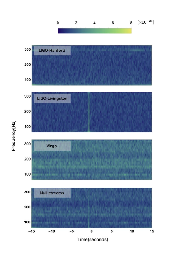
Figure 9: Time-frequency representations for the GW170817 GW170817-data : From top to bottom, aLIGO-Hanford, aLIGO-Livingston, and Virgo and the null stream $|P_{a}S_{a}|$ for the HLV network, where the arrival time at aLIGO-Hanford (and Virgo) is shifted with respect to aLIGO-Livingston. Times are shown relative to August 17, 2017 12:41:04 UTC. The vertical line (yellow green in color) around $-0.7$ seconds is due to the glitch which is a brief burst of instrumental noise a few seconds prior to event peak at aLIGO-Livingston, where the coalescence time is at time 0.4 seconds in this figure GW170817 . A horizontal striped pattern (light green in color) is due to noises at each detector. No chirp-like events are seen above the level of $\sim 2\times 10^{-23}$ in the null streams.

- (1) A. Einstein, Sitzungsber. Preuss. Akad. Wiss. Berlin (Math. Phys.) 1916, 688 (1916).
- (2) A. Einstein, Sitzungsber. Preuss. Akad. Wiss. Berlin (Math. Phys.) 1918, 154 (1918).
- (3) B. P. Abbott, et al. (LIGO Scientific Collaboration and Virgo Collaboration), Phys. Rev. Lett. 119, 161101 (2017); B. P. Abbott, et al., Astrophys. J. Lett. 848, L12 (2017); B. P. Abbott, et al., Astrophys. J. Lett. 848, L13 (2017)
- (4) D. M. Eardley, D. L. Lee, A. P. Lightman, R. V. Wagoner, and C. M. Will, Phys. Rev. Lett. 30, 884 (1973).
- (5) E. Poisson, and C. M. Will, Gravity, (Cambridge Univ. Press, UK. 2014).
- (6) M. Isi, A. J. Weinstein, C. Mead, and M. Pitkin, Phys. Rev. D 91, 082002 (2015).
- (7) M. Isi, M. Pitkin, and A. J. Weinstein, Phys. Rev. D 96, 042001 (2017).
- (8) A. A. Svidzinsky, ArXiv:1712.07181.
- (9) B. P. Abbott, et al., Phys. Rev. Lett. 120, 031104 (2018).
- (10) A. Nishizawa, A. Taruya, K. Hayama, S. Kawamura, and M. A. Sakagami, Phys. Rev. D 79, 082002 (2009).
- (11) K. Hayama, and A. Nishizawa, Phys. Rev. D 87, 062003 (2013).
- (12) H. Takeda, A. Nishizawa, Y. Michimura, K. Nagano, K. Komori, M. Ando, and K. Hayama, Phys. Rev. D 98, 022008 (2018).
- (13) B. P. Abbott, Living. Rev. Relativ., 21, 3 (2018).
- (14) K. Chatziioannou, N. Yunes, and N. Cornish, Phys. Rev. D 86, 022004 (2012).
- (15) Y. Gürsel, and M. Tinto, Phys. Rev. D 40, 3884 (1989).
- (16) L. Wen, and B. F. Schutz, Class. Quant. Grav. 22, S1321 (2005).
- (17) S. Chatterji, A. Lazzarini, L. Stein, P. J. Sutton, A. Searle, and M. Tinto, Phys. Rev. D 74, 082005 (2006).
- (18) Y. Hagihara, N. Era, D. Iikawa, and H. Asada, Phys. Rev. D 98, 064035 (2018).
- (19) The present paper uses a notation as and for vector- and vector- modes, respectively.
- (20) B. F. Schutz, and M. Tinto, Mon. Not. R. Astr. Soc. 224, 131 (1987).
- (21) The present paper follows Chapter 13 in Poisson and Will PW to define the GW antenna patterns for six possible polarization modes. See Nishizawa et al. Nishizawa2009 and also a pioneering work for purely TT waves by Schutz and Tinto ST . Note that their definitions are slightly different from each other PW ; Nishizawa2009 .
- (22) This is true for current ground-based detectors. However, it is not true for, e.g. planned Einstein Telescope or LISA, where the arms are not at 90 degrees with respect to each other.
- (23) https://www.gw-openscience.org/catalog/GWTC-1-confident/html/
- (24) M. Vallisneri et al. ”The LIGO Open Science Center”, proceedings of the 10th LISA Symposium, University of Florida, Gainesville, May 18-23, 2014; also arxiv:1410.4839