Hyperbolic Image Embeddings

Abstract

Computer vision tasks such as image classification, image retrieval, and few-shot learning are currently dominated by Euclidean and spherical embeddings so that the final decisions about class belongings or the degree of similarity are made using linear hyperplanes, Euclidean distances, or spherical geodesic distances (cosine similarity). In this work, we demonstrate that in many practical scenarios, hyperbolic embeddings provide a better alternative.

1 Introduction

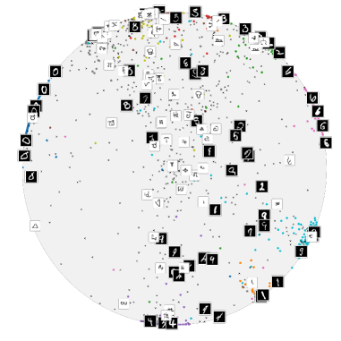
Figure 1: An example of two–dimensional Poincaré embeddings computed by a hyperbolic neural network trained on MNIST, and evaluated additionally on Omniglot. Ambiguous and unclear images from MNIST, as well as most of the images from Omniglot, are embedded near the center, while samples with clear class labels (or characters from Omniglot similar to one of the digits) lie near the boundary. *For inference, Omniglot was normalized to have the same background color as MNIST. Omniglot images are marked with black crosses, MNIST images with colored dots.

Learned high-dimensional embeddings are ubiquitous in modern computer vision. Learning aims to group together semantically-similar images and to separate semantically-different images. When the learning process is successful, simple classifiers can be used to assign an image to classes, and simple distance measures can be used to assess the similarity between images or image fragments. The operations at the end of deep networks imply a certain type of geometry of the embedding spaces. For example, image classification networks [19, 22] use linear operators (matrix multiplication) to map embeddings in the penultimate layer to class logits. The class boundaries in the embedding space are thus piecewise-linear, and pairs of classes are separated by Euclidean hyperplanes. The embeddings learned by the model in the penultimate layer, therefore, live in the Euclidean space. The same can be said about systems where Euclidean distances are used to perform image retrieval [31, 44, 58], face recognition [33, 57] or one-shot learning [43].

Alternatively, some few-shot learning [53], face recognition [41], and person re-identification methods [52, 59] learn spherical embeddings, so that sphere projection operator is applied at the end of a network that computes the embeddings. Cosine similarity (closely associated with sphere geodesic distance) is then used by such architectures to match images.

Euclidean spaces with their zero curvature and spherical spaces with their positive curvature have certain profound implications on the nature of embeddings that existing computer vision systems can learn. In this work, we argue that hyperbolic spaces with negative curvature might often be more appropriate for learning embedding of images. Towards this end, we add the recently-proposed hyperbolic network layers [11] to the end of several computer vision networks, and present a number of experiments corresponding to image classification, one-shot, and few-shot learning and person re-identification. We show that in many cases, the use of hyperbolic geometry improves the performance over Euclidean or spherical embeddings.

Our work is inspired by the recent body of works that demonstrate the advantage of learning hyperbolic embeddings for language entities such as taxonomy entries [29], common words [50], phrases [8] and for other NLP tasks, such as neural machine translation  [12]. Our results imply that hyperbolic spaces may be as valuable for improving the performance of computer vision systems.

Motivation for hyperbolic image embeddings.

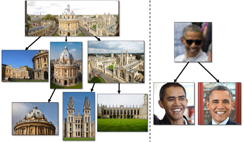
Figure 2: In many computer vision tasks, we want to learn image embeddings that obey the hierarchical constraints. E.g., in image retrieval (left), the hierarchy may arise from whole-fragment relation. In recognition tasks (right), the hierarchy can arise from image degradation, when degraded images are inherently ambiguous and may correspond to various identities/classes. Hyperbolic spaces are more suitable for embedding data with such hierarchical structure.

The use of hyperbolic spaces in natural language processing [29, 50, 8] is motivated by the ubiquity of hierarchies in NLP tasks. Hyperbolic spaces are naturally suited to embed hierarchies (e.g., tree graphs) with low distortion  [40, 39]. Here, we argue that hierarchical relations between images are common in computer vision tasks (Figure 2):

• In image retrieval, an overview photograph is related to many images that correspond to the close-ups of different distinct details. Likewise, for classification tasks in-the-wild, an image containing the representatives of multiple classes is related to images that contain representatives of the classes in isolation. Embedding a dataset that contains composite images into continuous space is, therefore, similar to embedding a hierarchy.

• In some tasks, more generic images may correspond to images that contain less information and are therefore more ambiguous. E.g., in face recognition, a blurry and/or low-resolution face image taken from afar can be related to many high-resolution images of faces that clearly belong to distinct people. Again natural embeddings for image datasets that have widely varying image quality/ambiguity calls for retaining such hierarchical structure.

• Many of the natural hierarchies investigated in natural language processing transcend to the visual domain. E.g., the visual concepts of different animal species may be amenable for hierarchical grouping (e.g. most felines share visual similarity while being visually distinct from pinnipeds).

Hierarchical relations between images call for the use of Hyperbolic spaces. Indeed, as the volume of hyperbolic spaces expands exponentially, it makes them continuous analogues of trees, in contrast to Euclidean spaces, where the expansion is polynomial. It therefore seems plausible that the exponentially expanding hyperbolic space will be able to capture the underlying hierarchy of visual data.

In order to build deep learning models which operate on the embeddings to hyperbolic spaces, we capitalize on recent developments  [11], which construct the analogues of familiar layers (such as a feed–forward layer, or a multinomial regression layer) in hyperbolic spaces. We show that many standard architectures used for tasks of image classification, and in particular in the few–shot learning setting can be easily modified to operate on hyperbolic embeddings, which in many cases also leads to their improvement.

The main contributions of our paper are twofold:

• First, we apply the machinery of hyperbolic neural networks to computer vision tasks. Our experiments with various few-shot learning and person re-identification models and datasets demonstrate that hyperbolic embeddings are beneficial for visual data.

• Second, we propose an approach to evaluate the hyperbolicity of a dataset based on the concept of Gromov $\delta$-hyperbolicity. It further allows estimating the radius of Poincaré disk for an embedding of a specific dataset and thus can serve as a handy tool for practitioners.

2 Related work

Hyperbolic language embeddings.

Hyperbolic embeddings in the natural language processing field have recently been very successful [29, 30]. They are motivated by the innate ability of hyperbolic spaces to embed hierarchies (e.g.,  tree graphs) with low distortion [39, 40]. However, due to the discrete nature of data in NLP, such works typically employ Riemannian optimization algorithms in order to learn embeddings of individual words to hyperbolic space. This approach is difficult to extend to visual data, where image representations are typically computed using CNNs.

Another direction of research, more relevant to the present work, is based on imposing hyperbolic structure on activations of neural networks [11, 12]. However, the proposed architectures were mostly evaluated on various NLP tasks, with correspondingly modified traditional models such as RNNs or Transformers. We find that certain computer vision problems that heavily use image embeddings can benefit from such hyperbolic architectures as well. Concretely, we analyze the following tasks.

Few–shot learning.

The task of few–shot learning is concerned with the overall ability of the model to generalize to unseen data during training. Most of the existing state-of-the-art few–shot learning models are based on metric learning approaches, utilizing the distance between image representations computed by deep neural networks as a measure of similarity [53, 43, 48, 28, 4, 6, 23, 2, 38, 5]. In contrast, other models apply meta-learning to few-shot learning: e.g., MAML by  [9], Meta-Learner LSTM by  [35], SNAIL by  [27]. While these methods employ either Euclidean or spherical geometries (like in  [53]), there was no extension to hyperbolic spaces.

Person re-identification.

The task of person re-identification is to match pedestrian images captured by possibly non-overlapping surveillance cameras. Papers [1, 13, 56] adopt the pairwise models that accept pairs of images and output their similarity scores. The resulting similarity scores are used to classify the input pairs as being matching or non-matching. Another popular direction of work includes approaches that aim at learning a mapping of the pedestrian images to the Euclidean descriptor space. Several papers, e.g., [46, 59] use verification loss functions based on the Euclidean distance or cosine similarity. A number of methods utilize a simple classification approach for training [3, 45, 17, 60], and Euclidean distance is used in test time.

3 Reminder on hyperbolic spaces and hyperbolicity estimation.

Formally, $n$-dimensional hyperbolic space denoted as $\mathbb{H}^{n}$ is defined as the homogeneous, simply connected $n$-dimensional Riemannian manifold of constant negative sectional curvature. The property of constant negative curvature makes it analogous to the ordinary Euclidean sphere (which has constant positive curvature); however, the geometrical properties of the hyperbolic space are very different. It is known that hyperbolic space cannot be isometrically embedded into Euclidean space  [18, 24], but there exist several well–studied models of hyperbolic geometry. In every model, a certain subset of Euclidean space is endowed with a hyperbolic metric; however, all these models are isomorphic to each other, and we may easily move from one to another base on where the formulas of interest are easier. We follow the majority of NLP works and use the Poincaré ball model.

The Poincaré ball model $(\mathbb{D}^{n},g^{\mathbb{D}})$ is defined by the manifold $\mathbb{D}^{n}=\{\mathbf{x}\in\mathbb{R}^{n}\colon\|\mathbf{x}\|<1\}$ endowed with the Riemannian metric $g^{\mathbb{D}}(\mathbf{x})=\lambda_{\mathbf{x}}^{2}g^{E}$, where $\lambda_{\mathbf{x}}=\frac{2}{1-\|\mathbf{x}\|^{2}}$ is the conformal factor and $g^{E}$ is the Euclidean metric tensor $g^{E}=\mathbf{I}^{n}$. In this model the geodesic distance between two points is given by the following expression:

$$d_{\mathbb{D}}(\mathbf{x},\mathbf{y})=\operatorname{arccosh}\Big{(}1+2\frac{\|\mathbf{x}-\mathbf{y}\|^{2}}{(1-\|\mathbf{x}\|^{2})(1-\|\mathbf{y}\|^{2})}\Big{)}.$$ (1)

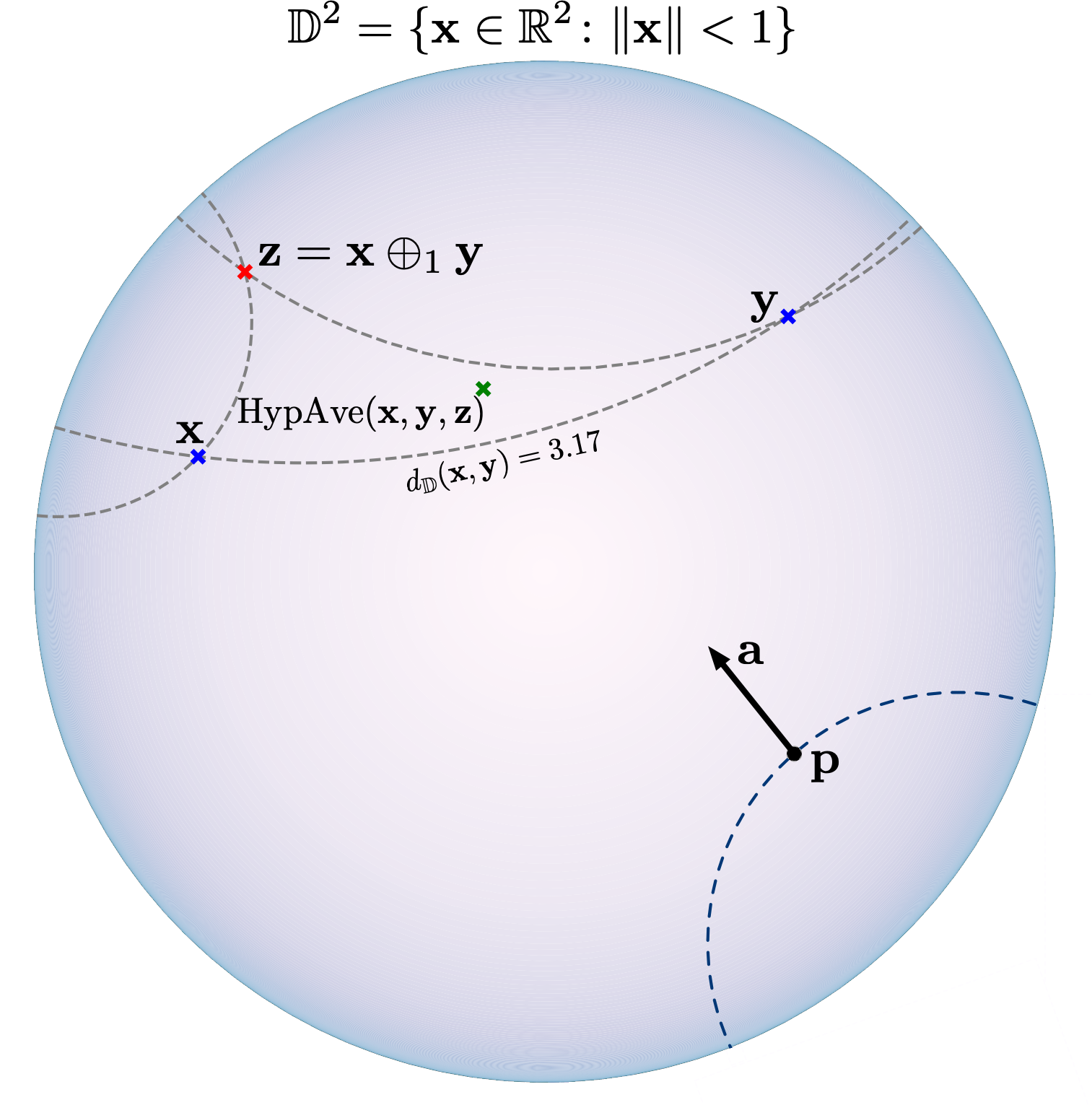
Figure 3: Visualization of the two–dimensional Poincaré ball. Point $\mathbf{z}$ represents the Möbius sum of points $\mathbf{x}$ and $\mathbf{y}$. $\mathrm{HypAve}$ stands for hyperbolic averaging. Gray lines represent geodesics, curves of shortest length connecting two points. In order to specify the hyperbolic hyperplanes (bottom), used for multiclass logistic regression, one has to provide an origin point $\mathbf{p}$ and a normal vector $\mathbf{a}\in T_{\mathbf{p}}\mathbb{D}^{2}\setminus\{\mathbf{0}\}$. For more details on hyperbolic operations see Section 4.

In order to define the hyperbolic average, we will make use of the Klein model of hyperbolic space. Similarly to the Poincaré model, it is defined on the set $\mathbb{K}^{n}=\{\mathbf{x}\in\mathbb{R}^{n}:\|\mathbf{x}\|<1\}$, however, with a different metric, not relevant for further discussion. In Klein coordinates, the hyperbolic average (generalizing the usual Euclidean mean) takes the most simple form, and we present the necessary formulas in Section 4.

From the viewpoint of hyperbolic geometry, all points of Poincaré ball are equivalent. The models that we consider below are, however, hybrid in the sense that most layers use Euclidean operators, such as standard generalized convolutions, while only the final layers operate within the hyperbolic geometry framework. The hybrid nature of our setups makes the origin a special point, since, from the Euclidean viewpoint, the local volumes in Poincare ball expand exponentially from the origin to the boundary. This leads to the useful tendency of the learned embeddings to place more generic/ambiguous objects closer to the origin while moving more specific objects towards the boundary. The distance to the origin in our models, therefore, provides a natural estimate of uncertainty, that can be used in several ways, as we show below.

This choice is justified for the following reasons. First, many existing vision architectures are designed to output embeddings in the vicinity of zero (e.g., in the unit ball). Another appealing property of hyperbolic space (assuming the standard Poincare ball model) is the existence of a reference point – the center of the ball. We show that in image classification which construct embeddings in the Poincare model of hyperbolic spaces the distance to the center can serve as a measure of confidence of the model — the input images which are more familiar to the model get mapped closer to the boundary, and images which confuse the model (e.g., blurry or noisy images, instances of a previously unseen class) are mapped closer to the center. The geometrical properties of hyperbolic spaces are quite different from the properties of the Euclidean space. For instance, the sum of angles of a geodesic triangle is always less than $\pi$. These interesting geometrical properties make it possible to construct a “score” which for an arbitrary metric space provides a degree of similarity of this metric space to a hyperbolic space. This score is called $\delta$-hyperbolicity, and we now discuss it in detail.

3.1 $\delta$-Hyperbolicity

Let us start with an illustrative example. The simplest discrete metric space possessing hyperbolic properties is a tree (in the sense of graph theory) endowed with the natural shortest path distance. Note the following property: for any three vertices $a,b,c$, the geodesic triangle (consisting of geodesics — paths of shortest length connecting each pair) spanned by these vertices (see Figure 4) is slim, which informally means that it has a center (vertex $d$) which is contained in every side of the triangle. By relaxing this condition to allow for some slack value $\delta$ and considering so-called $\delta$-slim triangles, we arrive at the following general definition.

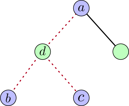
Figure 4: Visualization of a geodesic triangle in a tree. Such a tree endowed with a natural shortest path metric is a $0$–Hyperbolic space.

Table 1: Comparison of the theoretical degree of hyperbolicity with the relative delta $\delta_{rel}$ values estimated using Equations 2 and 4. The numbers are given for the two-dimensional Poincaré ball $\mathbb{D}^{2}$, the 2D sphere $S_{2}$, the upper hemisphere $S_{2}^{+}$, and a (random) tree graph.

	$\mathbb{D}^{2}$	$S_{2}^{+}$	$S_{2}$	Tree
Theory	$0$	$1$	$1$	$0$
$\delta_{rel}$	$0.18\pm 0.08$	$0.86\pm 0.11$	$0.97\pm 0.13$	$0.0$

Table 2: The relative delta $\delta_{rel}$ values calculated for different datasets. For image datasets we measured the Euclidean distance between the features produced by various standard feature extractors pretrained on ImageNet. Values of $\delta_{rel}$ closer to $0$ indicate a stronger hyperbolicity of a dataset. Results are averaged across $10$ subsamples of size $1000$. The standard deviation for all the experiments did not exceed $0.02$.

Encoder	Dataset
	CIFAR10	CIFAR100	CUB	MiniImageNet
Inception v3 [49]	$0.25$	$0.23$	$0.23$	$0.21$
ResNet34 [14]	$0.26$	$0.25$	$0.25$	$0.21$
VGG19 [42]	$0.23$	$0.22$	$0.23$	$0.17$

Let $X$ be an arbitrary (metric) space endowed with the distance function $d$. Its $\delta$-hyperbolicity value then may be computed as follows. We start with the so-called Gromov product for points $x,y,z\in X$:

$$(y,z)_{x}=\frac{1}{2}(d(x,y)+d(x,z)-d(y,z)).$$ (2)

Then, $\delta$ is defined as the minimal value such that the following four-point condition holds for all points $x,y,z,w\in X$:

$$(x,z)_{w}\geq\min((x,y)_{w},(y,z)_{w})-\delta.$$ (3)

The definition of hyperbolic space in terms of the Gromov product can be seen as saying that the metric relations between any four points are the same as they would be in a tree, up to the additive constant $\delta$. $\delta$-Hyperbolicity captures the basic common features of “negatively curved” spaces like the classical real-hyperbolic space $\mathbb{D}^{n}$ and of discrete spaces like trees.

For practical computations, it suffices to find the $\delta$ value for some fixed point $w=w_{0}$ as it is independent of $w$. An efficient way to compute $\delta$ is presented in [10]. Having a set of points, we first compute the matrix $A$ of pairwise Gromov products using Equation 2. After that, the $\delta$ value is simply the largest coefficient in the matrix $(A\otimes A)-A$, where $\otimes$ denotes the min-max matrix product

$${}A\otimes B=\max_{k}\min\{A_{ik},B_{kj}\}.$$ (4)

Results.

In order to verify our hypothesis on hyperbolicity of visual datasets we compute the scale-invariant metric, defined as $\delta_{rel}(X)=\frac{2\delta(X)}{\mathrm{diam}(X)}$, where $\mathrm{diam}(X)$ denotes the set diameter (maximal pairwise distance). By construction, $\delta_{rel}(X)\in[0,1]$ and specifies how close is a dataset to a hyperbolic space. Due to computational complexities of Equations 2 and 4 we employ the batched version of the algorithm, simply sampling $N$ points from a dataset, and finding the corresponding $\delta_{rel}$. Results are averaged across multiple runs, and we provide resulting mean and standard deviation. We experiment on a number of toy datasets (such as samples from the standard two–dimensional unit sphere), as well as on a number of popular computer vision datasets. As a natural distance between images, we used the standard Euclidean distance between feature vectors extracted by various CNNs pretrained on the ImageNet (ILSVRC) dataset [7]. Specifically, we consider VGG19 [42], ResNet34 [14] and Inception v3 [49] networks for distance evaluation. While other metrics are possible, we hypothesize that the underlying hierarchical structure (useful for computer vision tasks) of image datasets can be well understood in terms of their deep feature similarity.

Our results are summarized in Table 2. We observe that the degree of hyperbolicity in image datasets is quite high, as the obtained $\delta_{rel}$ are significantly closer to $0$ than to $1$ (which would indicate complete non-hyperbolicity). This observation suggests that visual tasks can benefit from hyperbolic representations of images.

Relation between $\delta$-hyperbolicity and Poincaré disk radius.

It is known [50] that the standard Poincaré ball is $\delta$-hyperbolic with $\delta_{P}=\log(1+\sqrt{2})\approx 0.88$. Formally, the diameter of the Poincaré ball is infinite, which yields the $\delta_{rel}$ value of $0$. However, from computational point of view we cannot approach the boundary infinitely close. Thus, we can compute the effective value of $\delta_{rel}$ for the Poincaré ball. For the clipping value of $10^{-5}$, i.e., when we consider only the subset of points with the (Euclidean) norm not exceeding $1-10^{-5}$, the resulting diameter is equal to $\sim 12.204$. This provides the effective $\delta_{rel}\approx 0.144$. Using this constant we can estimate the radius of Poincaré disk suitable for an embedding of a specific dataset. Suppose that for some dataset $X$ we have found that its $\delta_{rel}$ is equal to $\delta_{X}$. Then we can estimate $c(X)$ as follows.

$$c(X)=\Big{(}\frac{0.144}{\delta_{X}}\Big{)}^{2}.$$ (5)

For the previously studied datasets, this formula provides an estimate of $c\sim 0.33$. In our experiments, we found that this value works quite well; however, we found that sometimes adjusting this value (e.g., to $0.05$) provides better results, probably because the image representations computed by deep CNNs pretrained on ImageNet may not have been entirely accurate.

4 Hyperbolic operations

Hyperbolic spaces are not vector spaces in a traditional sense; one cannot use standard operations as summation, multiplication, etc. To remedy this problem, one can utilize the formalism of Möbius gyrovector spaces allowing to generalize many standard operations to hyperbolic spaces. Recently proposed hyperbolic neural networks adopt this formalism to define the hyperbolic versions of feed-forward networks, multinomial logistic regression, and recurrent neural networks  [11]. In Appendix  A, we discuss these networks and layers in detail, and in this section, we briefly summarize various operations available in the hyperbolic space. Similarly to the paper [11], we use an additional hyperparameter $c$ which modifies the curvature of Poincaré ball; it is then defined as $\mathbb{D}_{c}^{n}=\{\mathbf{x}\in\mathbb{R}^{n}:c\|\mathbf{x}\|^{2}<1,c\geq 0\}$. The corresponding conformal factor now takes the form $\lambda_{\mathbf{x}}^{c}=\frac{2}{1-c\|\mathbf{x}\|^{2}}$. In practice, the choice of $c$ allows one to balance between hyperbolic and Euclidean geometries, which is made precise by noting that with $c\to 0$, all the formulas discussed below take their usual Euclidean form. The following operations are the main building blocks of hyperbolic networks.

Möbius addition.

For a pair $\mathbf{x},\mathbf{y}\in\mathbb{D}_{c}^{n}$, the Möbius addition is defined as follows:

$$\mathbf{x}\oplus_{c}\mathbf{y}\coloneqq\frac{(1+2c\langle\mathbf{x},\mathbf{y}\rangle+c\|\mathbf{y}\|^{2})\mathbf{x}+(1-c\|\mathbf{x}\|^{2})\mathbf{y}}{1+2c\langle\mathbf{x},\mathbf{y}\rangle+c^{2}\|\mathbf{x}\|^{2}\|\mathbf{y}\|^{2}}.$$ (6)

Distance.

The induced distance function is defined as

$$d_{c}(\mathbf{x},\mathbf{y})\coloneqq\frac{2}{\sqrt{c}}\mathrm{arctanh}(\sqrt{c}\|-\mathbf{x}\oplus_{c}\mathbf{y}\|).$$ (7)

Note that with $c=1$ one recovers the geodesic distance (1), while with $c\to 0$ we obtain the Euclidean distance $\lim_{c\to 0}d_{c}(\mathbf{x},\mathbf{y})=2\|\mathbf{x}-\mathbf{y}\|.$

Exponential and logarithmic maps.

To perform operations in the hyperbolic space, one first needs to define a bijective map from $\mathbb{R}^{n}$ to $\mathbb{D}_{c}^{n}$ in order to map Euclidean vectors to the hyperbolic space, and vice versa. The so-called exponential and (inverse to it) logarithmic map serves as such a bijection.

The exponential map $\exp_{\mathbf{x}}^{c}$ is a function from $T_{\mathbf{x}}\mathbb{D}_{c}^{n}\cong\mathbb{R}^{n}$ to $\mathbb{D}_{c}^{n}$, which is given by

$$\exp_{\mathbf{x}}^{c}(\mathbf{v})\coloneqq\mathbf{x}\oplus_{c}\bigg{(}\tanh\bigg{(}\sqrt{c}\frac{\lambda_{\mathbf{x}}^{c}\|\mathbf{v}\|}{2}\bigg{)}\frac{\mathbf{v}}{\sqrt{c}\|\mathbf{v}\|}\bigg{)}.$$ (8)

The inverse logarithmic map is defined as

$$\log_{\mathbf{x}}^{c}(\mathbf{y})\coloneqq\frac{2}{\sqrt{c}\lambda_{\mathbf{x}}^{c}}\mathrm{arctanh}(\sqrt{c}\|-\mathbf{x}\oplus_{c}\mathbf{y}\|)\frac{-\mathbf{x}\oplus_{c}\mathbf{y}}{\|-\mathbf{x}\oplus_{c}\mathbf{y}\|}.$$ (9)

In practice, we use the maps $\exp_{\mathbf{0}}^{c}$ and $\log_{\mathbf{0}}^{c}$ for a transition between the Euclidean and Poincaré ball representations of a vector.

Hyperbolic averaging.

One important operation common in image processing is averaging of feature vectors, used, e.g., in prototypical networks for few–shot learning  [43]. In the Euclidean setting this operation takes the form $(\mathbf{x}_{1},\dots,\mathbf{x}_{N})\to\frac{1}{N}\sum_{i}\mathbf{x}_{i}$. Extension of this operation to hyperbolic spaces is called the Einstein midpoint and takes the most simple form in Klein coordinates:

$$\mathrm{HypAve}(\mathbf{x}_{1},\dots,\mathbf{x}_{N})=\sum_{i=1}^{N}\gamma_{i}\mathbf{x}_{i}/\sum_{i=1}^{N}\gamma_{i},$$ (10)

where $\gamma_{i}=\frac{1}{\sqrt{1-c\|\mathbf{x}_{i}\|^{2}}}$ are the Lorentz factors. Recall from the discussion in Section 3 that the Klein model is supported on the same space as the Poincaré ball; however, the same point has different coordinate representations in these models. Let $\mathbf{x}_{\mathbb{D}}$ and $\mathbf{x}_{\mathbb{K}}$ denote the coordinates of the same point in the Poincaré and Klein models correspondingly. Then the following transition formulas hold.

$$\mathbf{x}_{\mathbb{D}} =\frac{\mathbf{x}_{\mathbb{K}}}{1+\sqrt{1-c\|\mathbf{x}_{\mathbb{K}}\|^{2}}},$$ (11)

$$\mathbf{x}_{\mathbb{K}} =\frac{2\mathbf{x}_{\mathbb{D}}}{1+c\|\mathbf{x}_{\mathbb{D}}\|^{2}}.$$ (12)

Thus, given points in the Poincaré ball, we can first map them to the Klein model, compute the average using Equation (10), and then move it back to the Poincaré model.

Numerical stability.

While implementing most of the formulas described above is straightforward, we employ some tricks to make the training more stable. In particular, to ensure numerical stability, we perform clipping by norm after applying the exponential map, which constrains the norm not to exceed $\frac{1}{\sqrt{c}}(1-10^{-3})$.

5 Experiments

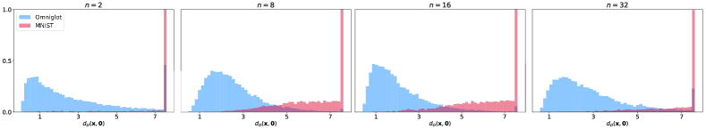
Figure 5: Distributions of the hyperbolic distance to the origin of the MNIST (red) and Omniglot (blue) datasets embedded into the Poincaré ball; parameter $n$ denotes embedding dimension of the model trained for MNIST classification. Most Omniglot instances can be easily identified as out-of-domain based on their distance to the origin.

Experimental setup.

We start with a toy experiment supporting our hypothesis that the distance to the center in Poincaré ball indicates a model uncertainty. To do so, we first train a classifier in hyperbolic space on the MNIST dataset  [21] and evaluate it on the Omniglot dataset  [20]. We then investigate and compare the obtained distributions of distances to the origin of hyperbolic embeddings of the MNIST and Omniglot test sets.

In our further experiments, we concentrate on the few-shot classification and person re-identification tasks. The experiments on the Omniglot dataset serve as a starting point, and then we move towards more complex datasets. Afterwards, we consider two datasets, namely: MiniImageNet  [35] and Caltech-UCSD Birds-200-2011 (CUB)  [54]. Finally, we provide the re-identification results for the two popular datasets: Market-1501  [61] and DukeMTMD  [36, 62]. Further in this section, we provide a thorough description of each experiment. Our code is available at github.

Table 3: Kolmogorov-Smirnov distances between the distributions of distance to the origin of the MNIST and Omniglot datasets embedded into the Poincaré ball with the hyperbolic classifier trained on MNIST, and between the distributions of $p_{\max}$ (maximum probablity predicted for a class) for the Euclidean classifier trained on MNIST and evaluated on the same sets.

	$n=2$	$n=8$	$n=16$	$n=32$
$d_{\mathbb{D}}(\mathbf{x},\mathbf{0})$	$\mathbf{0.868}$	$0.832$	$\mathbf{0.853}$	$\mathbf{0.859}$
$p_{\max}(\mathbf{x})$	$0.834$	$\mathbf{0.835}$	$0.840$	$0.846$

5.1 Distance to the origin as the measure of uncertainty

In this subsection, we validate our hypothesis, which claims that if one trains a hyperbolic classifier, then the distance of the Poincaré ball embedding of an image to the origin can serve as a good measure of confidence of a model. We start by training a simple hyperbolic convolutional neural network on the MNIST dataset (we hypothesized that such a simple dataset contains a very basic hierarchy, roughly corresponding to visual ambiguity of images, as demonstrated by a trained network on Figure 1). The output of the last hidden layer was mapped to the Poincaré ball using the exponential map (8) and was followed by the hyperbolic multi-linear regression (MLR) layer [11].

After training the model to $\sim 99\%$ test accuracy, we evaluate it on the Omniglot dataset (by resizing its images to $28\times 28$ and normalizing them to have the same background color as MNIST). We then evaluated the hyperbolic distance to the origin of embeddings produced by the network on both datasets. The closest Euclidean analogue to this approach would be comparing distributions of $p_{\max}$, maximum class probability predicted by the network. For the same range of dimensions, we train ordinary Euclidean classifiers on MNIST and compare these distributions for the same sets. Our findings are summarized in Figure 5 and Table 3. We observe that distances to the origin represent a better indicator of the dataset dissimilarity in three out of four cases.

We have visualized the learned MNIST and Omniglot embeddings in Figure 1. We observe that more “unclear” images are located near the center, while the images that are easy to classify are located closer to the boundary.

5.2 Few–shot classification

We hypothesize that a certain class of problems — namely the few-shot classification task can benefit from hyperbolic embeddings, due to the ability of hyperbolic space to accurately reflect even very complex hierarchical relations between data points. In principle, any metric learning approach can be modified to incorporate the hyperbolic embeddings. We decided to focus on the classical approach called prototypical networks (ProtoNets) introduced in  [43]. This approach was picked because it is simple in general and simple to convert to hyperbolic geometry. ProtoNets use the so-called prototype representation of a class, which is defined as a mean of the embedded support set of a class. Generalizing this concept to hyperbolic space, we substitute the Euclidean mean operation by $\mathrm{HypAve}$, defined earlier in (10). We show that Hyperbolic ProtoNets can achieve results competitive with many recent state-of-the-art models. Our main experiments are conducted on MiniImageNet and Caltech-UCSD Birds-200-2011 (CUB). Additional experiments on the Omniglot dataset, as well as the implementation details and hyperparameters, are provided in Appendix B. For a visualization of learned embeddings see Appendix C.

MiniImageNet.

MiniImageNet dataset is the subset of ImageNet dataset  [37] that contains $100$ classes represented by $600$ examples per class. We use the following split provided in the paper  [35]: the training dataset consists of $64$ classes, the validation dataset is represented by $16$ classes, and the remaining $20$ classes serve as the test dataset. We test the models on tasks for 1-shot and 5-shot classifications; the number of query points in each batch always equals to $15$. Similarly to [43], the model is trained in the 30-shot regime for the 1-shot task and the 20-shot regime for the 1-shot task. We test our approach with two different backbone CNN models: a commonly used four-block CNN [43, 4] (denoted ‘4 Conv’ in the table) and ResNet18 [14]. To find the best values of hyperparameters, we used the grid search; see Appendix B for the complete list of values.

Table 4: Few-shot classification accuracy results on MiniImageNet on 1-shot 5-way and 5-shot 5-way tasks. All accuracy results are reported with 95% confidence intervals.

Baselines	Embedding Net	1-Shot 5-Way	5-Shot 5-Way
MatchingNet [53]	4 Conv	43.56 $\pm$ 0.84%	55.31 $\pm$ 0.73%
MAML [9]	4 Conv	48.70 $\pm$ 1.84%	63.11 $\pm$ 0.92%
RelationNet [48]	4 Conv	50.44 $\pm$ 0.82%	65.32 $\pm$ 0.70%
REPTILE [28]	4 Conv	49.97 $\pm$ 0.32%	65.99 $\pm$ 0.58%
ProtoNet [43]	4 Conv	49.42 $\pm$ 0.78%	68.20 $\pm$ 0.66%
Baseline* [4]	4 Conv	41.08 $\pm$ 0.70%	54.50 $\pm$ 0.66%
Spot&learn [6]	4 Conv	51.03 $\pm$ 0.78%	67.96 $\pm$ 0.71%
DN4 [23]	4 Conv	51.24 $\pm$ 0.74%	71.02 $\pm$ 0.64%
Hyperbolic ProtoNet	4 Conv	54.43 $\pm$ 0.20%	72.67 $\pm$ 0.15%
SNAIL [27]	ResNet12	55.71 $\pm$ 0.99%	68.88 $\pm$ 0.92%
ProtoNet+ [43]	ResNet12	56.50 $\pm$ 0.40%	74.2 $\pm$ 0.20%
CAML [16]	ResNet12	59.23 $\pm$ 0.99%	72.35 $\pm$ 0.71%
TPN [25]	ResNet12	59.46%	75.65%
MTL [47]	ResNet12	61.20 $\pm$ 1.8%	75.50 $\pm$ 0.8%
DN4 [23]	ResNet12	54.37 $\pm$ 0.36%	74.44 $\pm$ 0.29%
TADAM [32]	ResNet12	58.50%	76.70%
Qiao-WRN [34]	Wide-ResNet28	59.60 $\pm$ 0.41%	73.74 $\pm$ 0.19%
LEO [38]	Wide-ResNet28	61.76 $\pm$ 0.08%	77.59 $\pm$ 0.12%
Dis. k-shot [2]	ResNet34	56.30 $\pm$ 0.40%	73.90 $\pm$ 0.30%
Self-Jig(SVM) [5]	ResNet50	58.80 $\pm$ 1.36%	76.71 $\pm$ 0.72%
Hyperbolic ProtoNet	ResNet18	59.47 $\pm$ 0.20%	76.84 $\pm$ 0.14%

Table 4 illustrates the obtained results on the MiniImageNet dataset (alongside other results in the literature). Interestingly, Hyperbolic ProtoNet significantly improves accuracy as compared to the standard ProtoNet, especially in the one-shot setting. We observe that the obtained accuracy values, in many cases, exceed the results obtained by more advanced methods, sometimes even in the case of architecture of larger capacity. This partly confirms our hypothesis that hyperbolic geometry indeed allows for more accurate embeddings in the few–shot setting.

Caltech-UCSD Birds.

The CUB dataset consists of $11,788$ images of $200$ bird species and was designed for fine-grained classification. We use the split introduced in  [51]: $100$ classes out of $200$ were used for training, $50$ for validation and $50$ for testing. Due to the relative simplicity of the dataset, we consider only the 4-Conv backbone and do not modify the training shot values as was done for the MiniImageNet case. The full list of hyperparameters is provided in Appendix B.

Our findings are summarized in Table 5. Interestingly, for this dataset, the hyperbolic version of ProtoNet significantly outperforms its Euclidean counterpart (by more than 10% in both settings), and outperforms many other algorithms.

Table 5: Few-shot classification accuracy results on CUB dataset [55] on 1-shot 5-way task, 5-shot 5-way task. All accuracy results are reported with 95% confidence intervals. For each task, the best-performing method is highlighted.

Baselines	Embedding Net	1-Shot 5-Way	5-Shot 5-Way
MatchingNet [53]	4 Conv	61.16 $\pm$ 0.89	72.86 $\pm$ 0.70
MAML [9]	4 Conv	55.92 $\pm$ 0.95%	72.09 $\pm$ 0.76%
ProtoNet [43]	4 Conv	51.31 $\pm$ 0.91%	70.77 $\pm$ 0.69%
MACO [15]	4 Conv	60.76%	74.96%
RelationNet [48]	4 Conv	62.45 $\pm$ 0.98%	76.11 $\pm$ 0.69%
Baseline++ [4]	4 Conv	60.53 $\pm$ 0.83%	79.34 $\pm$ 0.61%
DN4-DA [23]	4 Conv	53.15 $\pm$ 0.84%	81.90 $\pm$ 0.60%
Hyperbolic ProtoNet	4 Conv	64.02 $\pm$ 0.24%	82.53 $\pm$ 0.14%

5.3 Person re-identification

Table 6: Person re-identification results for Market-1501 and DukeMTMC-reID for the classification baseline (Euclidean) and its hyperbolic counterpart (Hyperbolic). (See 5.3 for the details). The results are shown for the three embedding dimensionalities and for two different learning rate schedules. For each dataset and each embedding dimensionality value, the best results are bold, they are all given by the hyperbolic version of classification (either by the schedule sch#1 or sch#2). The second-best results are underlined.

	Market-1501				DukeMTMC-reID
	Euclidean		Hyperbolic		Euclidean		Hyperbolic
dim, lr schedule	r1	mAP	r1	mAP	r1	mAP	r1	mAP
32, sch#1	71.4	49.7	69.8	45.9	56.1	35.6	56.5	34.9
32, sch#2	68.0	43.4	75.9	51.9	57.2	35.7	62.2	39.1
64, sch#1	80.3	60.3	83.1	60.1	69.9	48.5	70.8	48.6
64, sch#2	80.5	57.8	84.4	62.7	68.3	45.5	70.7	48.6
128, sch#1	86.0	67.3	87.8	68.4	74.1	53.3	76.5	55.4
128, sch#2	86.5	68.5	86.4	66.2	71.5	51.5	74.0	52.2

The DukeMTMC-reID dataset [36, 62] contains $16,522$ training images of $702$ identities, $2,228$ query images of $702$ identities and $17,661$ gallery images. The Market1501 dataset [61] contains $12,936$ training images of $751$ identities, $3,368$ queries of $750$ identities and $15,913$ gallery images respectively. We report Rank1 of the Cumulative matching Characteristic Curve and Mean Average Precision for both datasets. The results (Table 6) are reported after the $300$ training epochs. The experiments were performed with the ResNet50 backbone, and two different learning rate schedulers (see Appendix B for more details). The hyperbolic version generally performs better than the Euclidean baseline, with the advantage being bigger for smaller dimensionality.

6 Discussion and conclusion

We have investigated the use of hyperbolic spaces for image embeddings. The models that we have considered use Euclidean operations in most layers, and use the exponential map to move from the Euclidean to hyperbolic spaces at the end of the network (akin to the normalization layers that are used to map from the Euclidean space to Euclidean spheres). The approach that we investigate here is thus compatible with existing backbone networks trained in Euclidean geometry.

At the same time, we have shown that across a number of tasks, in particular in the few-shot image classification, learning hyperbolic embeddings can result in a substantial boost in accuracy. We speculate that the negative curvature of the hyperbolic spaces allows for embeddings that are better conforming to the intrinsic geometry of at least some image manifolds with their hierarchical structure.

Future work may include several potential modifications of the approach. We have observed that the benefit of hyperbolic embeddings may be substantially bigger in some tasks and datasets than in others. A better understanding of when and why the use of hyperbolic geometry is warranted is therefore needed. Finally, we note that while all hyperbolic geometry models are equivalent in the continuous setting, fixed-precision arithmetic used in real computers breaks this equivalence. In practice, we observed that care should be taken about numeric precision effects. Using other models of hyperbolic geometry may result in a more favourable floating point performance.

Appendix A Hyperbolic Neural Networks

Linear layer.

Assume we have a standard (Euclidean) linear layer $\mathbf{x}\to\mathrm{M}\mathbf{x}+\mathbf{b}$. In order to generalize it, one needs to define the Möbius matrix by vector product:

$$\mathrm{M}^{\otimes_{c}}(\mathbf{x})\coloneqq\frac{1}{\sqrt{c}}\tanh\bigg{(}\frac{\|\mathrm{M}\mathbf{x}\|}{\|\mathbf{x}\|}\mathrm{arctanh}(\sqrt{c}\|\mathbf{x}\|)\bigg{)}\frac{\mathrm{M}\mathbf{x}}{\|\mathrm{M}\mathbf{x}\|},$$ (13)

if $\mathrm{M}\mathbf{x}\neq\mathbf{0}$, and $\mathrm{M}^{\otimes_{c}}(\mathbf{x})\coloneqq\mathbf{0}$ otherwise. Finally, for a bias vector $\mathbf{b}\in\mathbb{D}^{n}_{c}$ the operation underlying the hyperbolic linear layer is then given by $\mathrm{M}^{\otimes_{c}}(\mathbf{x})\oplus_{c}\mathbf{b}$.

Concatenation of input vectors.

In several architectures (e.g., in siamese networks), it is needed to concatenate two vectors; such operation is obvious in Euclidean space. However, straightforward concatenation of two vectors from hyperbolic space does not necessarily remain in hyperbolic space. Thus, we have to use a generalized version of the concatenation operation, which is then defined in the following manner. For $\mathbf{x}\in\mathbb{D}^{n_{1}}_{c}$, $\mathbf{y}\in\mathbb{D}^{n_{2}}_{c}$ we define the mapping $\mathrm{Concat}:\mathbb{D}^{n_{1}}_{c}\times\mathbb{D}^{n_{2}}_{c}\to\mathbb{D}^{n_{3}}_{c}$ as follows.

$${}\mathrm{Concat}(\mathbf{x},\mathbf{y})=\mathrm{M}_{1}^{\otimes_{c}}\mathbf{x}\oplus_{c}\mathrm{M}_{2}^{\otimes_{c}}\mathbf{y},$$ (14)

where $\mathrm{M}_{1}$ and $\mathrm{M}_{2}$ are trainable matrices of sizes $n_{3}\times n_{1}$ and $n_{3}\times n_{2}$ correspondingly. The motivation for this definition is simple: usually, the Euclidean concatenation layer is followed by a linear map, which when written explicitly takes the (Euclidean) form of Equation (14).

Multiclass logistic regression (MLR).

In our experiments, to perform the multiclass classification, we take advantage of the generalization of multiclass logistic regression to hyperbolic spaces. The idea of this generalization is based on the observation that in Euclidean space logits can be represented as the distances to certain hyperplanes, where each hyperplane can be specified with a point of origin and a normal vector. The same construction can be used in the Poincaré ball after a suitable analogue for hyperplanes is introduced. Given $\mathbf{p}\in\mathbb{D}_{c}^{n}$ and $\mathbf{a}\in T_{\mathbf{p}}\mathbb{D}_{c}^{n}\setminus\{\mathbf{0}\}$, such an analogue would be the union of all geodesics passing through $\mathbf{p}$ and orthogonal to $\mathbf{a}$.

The resulting formula for hyperbolic MLR for $K$ classes is written below; here $\mathbf{p}_{k}\in\mathbb{D}_{c}^{n}$ and $\mathbf{a}_{k}\in T_{\mathbf{p}_{k}}\mathbb{D}_{c}^{n}\setminus\{\mathbf{0}\}$ are learnable parameters.

$$\begin{split}p(y&=k|\mathbf{x})\propto\\ &\exp\bigg{(}\frac{\lambda_{\mathbf{p}_{k}}^{c}\|\mathbf{a}_{k}\|}{\sqrt{c}}\mathrm{arcsinh}\bigg{(}\frac{2\sqrt{c}\langle-\mathbf{p}_{k}\oplus_{c}\mathbf{x},\mathbf{a}_{k}\rangle}{(1-c\|-\mathbf{p}_{k}\oplus_{c}\mathbf{x}\|^{2})\|\mathbf{a}_{k}\|}\bigg{)}\bigg{)}.\end{split}$$

For a more thorough discussion of hyperbolic neural networks, we refer the reader to the paper  [11].

Appendix B Experiment details

Omniglot.

As a baseline model, we consider the prototype network (ProtoNet). Each convolutional block consists of $3\times 3$ convolutional layer followed by batch normalization, ReLU nonlinearity and $2\times 2$ max-pooling layer. The number of filters in the last convolutional layer corresponds to the value of the embedding dimension, for which we choose $64$. The hyperbolic model differs from the baseline in the following aspects. First, the output of the last convolutional block is embedded into the Poincaré ball of dimension $64$ using the exponential map. Results are presented in Table 7. We can see that in some scenarios, in particular for one-shot learning, hyperbolic embeddings are more beneficial, while in other cases, results are slightly worse. The relative simplicity of this dataset may explain why we have not observed a significant benefit of hyperbolic embeddings. We further test our approach on more advanced datasets.

Table 7: Few-shot classification accuracies on Omniglot. In order to obtain Hyperbolic ProtoNet, we augment the standard ProtoNet with a mapping to the Poincaré ball, use hyperbolic distance as the distance function, and as the averaging operator we use the $\mathrm{HypAve}$ operator defined by Equation (10).

	ProtoNet	Hyperbolic ProtoNet
$1$-shot $5$-way	$98.2$	$\mathbf{99.0}$
$5$-shot $5$-way	$99.4$	$99.4$
$1$-shot $20$-way	$95.8$	$\mathbf{95.9}$
$5$-shot $20$-way	$\mathbf{98.6}$	$98.15$

miniImageNet.

We performed the experiments with two different backbones, namely the previously discussed 4-Conv model and ResNet18. For the former, embedding dim was set to 1024 and for the latter to 512. For the one-shot setting both models were trained for $200$ epochs with Adam optimizer, learning rate being $5\cdot 10^{-3}$ and step learning rate decay with the factor of $0.5$ and step size being $80$ epochs. For the 4-Conv model we used $c=0.01$ and for ResNet18 we used $c=0.001$. For 4-Conv in the five-shot setting we used the same hyperparameters except for $c=0.005$ and learning rate decay step being $60$ epochs. For ResNet18 we additionally changed learning rate to $10^{-3}$ and step size to $40$.

Caltech-UCSD Birds.

For these experiments we used the same 4-Conv architecture with the embedding dimensionality being $512$. For the one-shot task, we used learning rate $10^{-3}$, $c=0.05$, learning rate step being $50$ epochs and decay rate of $0.8$. For the five-shot task, we used learning rate $10^{-3}$, $c=0.01$, learning rate step of $40$ and decay rate of $0.8$.

Person re-identification.

We use ResNet50  [14] architecture with one fully connected embedding layer following the global average pooling. Three embedding dimensionalities are used in our experiments: $32$, $64$ and $128$. For the baseline experiments, we add the additional classification linear layer, followed by the cross-entropy loss. For the hyperbolic version of the experiments, we map the descriptors to the Poincaré ball and apply multiclass logistic regression as described in Section 4. We found that in both cases the results are very sensitive to the learning rate schedules. We tried four schedules for learning $32$-dimensional descriptors for both baseline and hyperbolic versions. The two best performing schedules were applied for the $64$ and $128$-dimensional descriptors. In these experiments, we also found that smaller $c$ values give better results. We therefore have set $c$ to $10^{-5}$. Based on the discussion in 4, our hyperbolic setting is quite close to Euclidean. The results are compiled in Table 6. We set starting learning rates to $3\cdot 10^{-4}$ and $6\cdot 10^{-4}$ for $sch\#1$ and $sch\#2$ correspondingly and multiply them by $0.1$ after each of the epochs $200$ and $270$.

Appendix C Visualizations

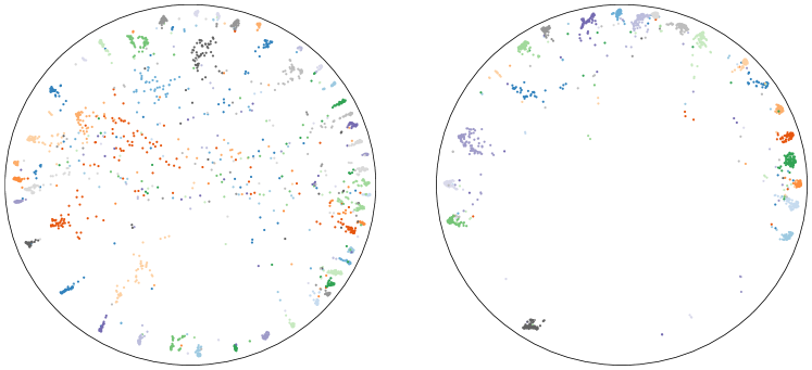
Figure 6: A visualization of the hyperbolic embeddings learned for the few–shot task. Left: 5-shot task on CUB. Right: 5-shot task on MiniImageNet. The two-dimensional projection was computed with the UMAP algorithm [26].

For the visual inspection of embeddings we computed projections of high dimensional embeddings obtained from the trained few–shot models with the (hyperbolic) UMAP algorithm [26] (see Figure 6). We observe that different classes are neatly positioned near the boundary of the circle and are well separated.

References

- [1] Ejaz Ahmed, Michael J. Jones, and Tim K. Marks. An improved deep learning architecture for person re-identification. In Conf. Computer Vision and Pattern Recognition, CVPR, pages 3908–3916, 2015.
- [2] Matthias Bauer, Mateo Rojas-Carulla, Jakub Bartlomiej Swiatkowski, Bernhard Scholkopf, and Richard E Turner. Discriminative k-shot learning using probabilistic models. arXiv preprint arXiv:1706.00326, 2017.
- [3] Xiaobin Chang, Timothy M Hospedales, and Tao Xiang. Multi-level factorisation net for person re-identification. In Proceedings of the IEEE Conference on Computer Vision and Pattern Recognition, pages 2109–2118, 2018.
- [4] Wei-Yu Chen, Yen-Cheng Liu, Zsolt Kira, Yu-Chiang Frank Wang, and Jia-Bin Huang. A closer look at few-shot classification. In ICLR, 2019.
- [5] Zitian Chen, Yanwei Fu, Kaiyu Chen, and Yu-Gang Jiang. Image block augmentation for one-shot learning. In AAAI, 2019.
- [6] Wen-Hsuan Chu, Yu-Jhe Li, Jing-Cheng Chang, and Yu-Chiang Frank Wang. Spot and learn: A maximum-entropy patch sampler for few-shot image classification. In CVPR, pages 6251–6260, 2019.
- [7] Jia Deng, Wei Dong, Richard Socher, Li-Jia Li, Kai Li, and Li Fei-Fei. Imagenet: A large-scale hierarchical image database. In CVPR, pages 248–255. IEEE, 2009.
- [8] Bhuwan Dhingra, Christopher J Shallue, Mohammad Norouzi, Andrew M Dai, and George E Dahl. Embedding text in hyperbolic spaces. arXiv preprint arXiv:1806.04313, 2018.
- [9] Chelsea Finn, Pieter Abbeel, and Sergey Levine. Model-agnostic meta-learning for fast adaptation of deep networks. In ICML, pages 1126–1135. JMLR, 2017.
- [10] Hervé Fournier, Anas Ismail, and Antoine Vigneron. Computing the Gromov hyperbolicity of a discrete metric space. Information Processing Letters, 115(6-8):576–579, 2015.
- [11] Octavian Ganea, Gary Bécigneul, and Thomas Hofmann. Hyperbolic neural networks. In Advances in Neural Information Processing Systems, pages 5350–5360, 2018.
- [12] Caglar Gulcehre, Misha Denil, Mateusz Malinowski, Ali Razavi, Razvan Pascanu, Karl Moritz Hermann, Peter Battaglia, Victor Bapst, David Raposo, Adam Santoro, and Nando de Freitas. Hyperbolic attention networks. In International Conference on Learning Representations, 2019.
- [13] Yiluan Guo and Ngai-Man Cheung. Efficient and deep person re-identification using multi-level similarity. In Proceedings of the IEEE Conference on Computer Vision and Pattern Recognition, pages 2335–2344, 2018.
- [14] Kaiming He, Xiangyu Zhang, Shaoqing Ren, and Jian Sun. Deep residual learning for image recognition. In Proceedings of the IEEE conference on computer vision and pattern recognition, pages 770–778, 2016.
- [15] Nathan Hilliard, Lawrence Phillips, Scott Howland, Artëm Yankov, Courtney D Corley, and Nathan O Hodas. Few-shot learning with metric-agnostic conditional embeddings. arXiv preprint arXiv:1802.04376, 2018.
- [16] Xiang Jiang, Mohammad Havaei, Farshid Varno, Gabriel Chartrand, Nicolas Chapados, and Stan Matwin. Learning to learn with conditional class dependencies. In ICLR, 2019.
- [17] Mahdi M Kalayeh, Emrah Basaran, Muhittin Gökmen, Mustafa E Kamasak, and Mubarak Shah. Human semantic parsing for person re-identification. In Proceedings of the IEEE Conference on Computer Vision and Pattern Recognition, pages 1062–1071, 2018.
- [18] Dmitri Krioukov, Fragkiskos Papadopoulos, Maksim Kitsak, Amin Vahdat, and Marián Boguná. Hyperbolic geometry of complex networks. Physical Review E, 82(3):036106, 2010.
- [19] Alex Krizhevsky, Ilya Sutskever, and Geoffrey E Hinton. Imagenet classification with deep convolutional neural networks. In Advances in Neural Information Processing Systems, pages 1097–1105, 2012.
- [20] Brenden M Lake, Ruslan R Salakhutdinov, and Josh Tenenbaum. One-shot learning by inverting a compositional causal process. In Advances in Neural Information Processing Systems, pages 2526–2534, 2013.
- [21] Yann LeCun, Léon Bottou, Yoshua Bengio, Patrick Haffner, et al. Gradient-based learning applied to document recognition. Proceedings of the IEEE, 86(11):2278–2324, 1998.
- [22] Yann LeCun et al. Generalization and network design strategies. In Connectionism in perspective, volume 19. Citeseer, 1989.
- [23] Wenbin Li, Lei Wang, Jinglin Xu, Jing Huo, Yang Gao, and Jiebo Luo. Revisiting local descriptor based image-to-class measure for few-shot learning. In CVPR, pages 7260–7268, 2019.
- [24] Nathan Linial, Avner Magen, and Michael E Saks. Low distortion Euclidean embeddings of trees. Israel Journal of Mathematics, 106(1):339–348, 1998.
- [25] Yanbin Liu, Juho Lee, Minseop Park, Saehoon Kim, Eunho Yang, Sungju Hwang, and Yi Yang. Learning To Propagate Labels: Transductive Propagation Network For Few-Shot Learning. In ICLR, 2019.
- [26] Leland McInnes, John Healy, and James Melville. Umap: Uniform manifold approximation and projection for dimension reduction. arXiv preprint arXiv:1802.03426, 2018.
- [27] Nikhil Mishra, Mostafa Rohaninejad, Xi Chen, and Pieter Abbeel. A simple neural attentive meta-learner. arXiv preprint arXiv:1707.03141, 2017.
- [28] Alex Nichol and John Schulman. Reptile: a scalable metalearning algorithm. arXiv preprint arXiv:1803.02999, 2, 2018.
- [29] Maximillian Nickel and Douwe Kiela. Poincaré embeddings for learning hierarchical representations. In Advances in Neural Information Processing Systems, pages 6338–6347, 2017.
- [30] Maximilian Nickel and Douwe Kiela. Learning continuous hierarchies in the Lorentz model of Hyperbolic geometry. In Proc. ICML, pages 3776–3785, 2018.
- [31] Hyun Oh Song, Yu Xiang, Stefanie Jegelka, and Silvio Savarese. Deep metric learning via lifted structured feature embedding. In Proceedings of the IEEE Conference on Computer Vision and Pattern Recognition, pages 4004–4012, 2016.
- [32] Boris Oreshkin, Pau Rodríguez López, and Alexandre Lacoste. Tadam: Task dependent adaptive metric for improved few-shot learning. In NeurIPS, pages 719–729, 2018.
- [33] O. M. Parkhi, A. Vedaldi, and A. Zisserman. Deep face recognition. In British Machine Vision Conference, 2015.
- [34] Siyuan Qiao, Chenxi Liu, Wei Shen, and Alan L Yuille. Few-shot image recognition by predicting parameters from activations. In CVPR, pages 7229–7238, 2018.
- [35] Sachin Ravi and Hugo Larochelle. Optimization as a model for few-shot learning. 2016.
- [36] Ergys Ristani, Francesco Solera, Roger Zou, Rita Cucchiara, and Carlo Tomasi. Performance measures and a data set for multi-target, multi-camera tracking. In European Conference on Computer Vision workshop on Benchmarking Multi-Target Tracking, 2016.
- [37] Olga Russakovsky, Jia Deng, Hao Su, Jonathan Krause, Sanjeev Satheesh, Sean Ma, Zhiheng Huang, Andrej Karpathy, Aditya Khosla, Michael Bernstein, et al. Imagenet large scale visual recognition challenge. International Journal of Computer Vision, 115(3):211–252, 2015.
- [38] Andrei A. Rusu, Dushyant Rao, Jakub Sygnowski, Oriol Vinyals, Razvan Pascanu, Simon Osindero, and Raia Hadsell. Meta-learning with latent embedding optimization. In ICLR, 2019.
- [39] Frederic Sala, Chris De Sa, Albert Gu, and Christopher Ré. Representation tradeoffs for hyperbolic embeddings. In International Conference on Machine Learning, pages 4457–4466, 2018.
- [40] Rik Sarkar. Low distortion Delaunay embedding of trees in hyperbolic plane. In International Symposium on Graph Drawing, pages 355–366. Springer, 2011.
- [41] Florian Schroff, Dmitry Kalenichenko, and James Philbin. Facenet: A unified embedding for face recognition and clustering. In Proceedings of the IEEE conference on computer vision and pattern recognition, pages 815–823, 2015.
- [42] Karen Simonyan and Andrew Zisserman. Very deep convolutional networks for large-scale image recognition. arXiv preprint arXiv:1409.1556, 2014.
- [43] Jake Snell, Kevin Swersky, and Richard Zemel. Prototypical networks for few-shot learning. In NeurIPS, pages 4077–4087, 2017.
- [44] Kihyuk Sohn. Improved deep metric learning with multi-class n-pair loss objective. In Advances in Neural Information Processing Systems, pages 1857–1865, 2016.
- [45] Chi Su, Jianing Li, Shiliang Zhang, Junliang Xing, Wen Gao, and Qi Tian. Pose-driven deep convolutional model for person re-identification. In Proceedings of the IEEE International Conference on Computer Vision, pages 3960–3969, 2017.
- [46] Yumin Suh, Jingdong Wang, Siyu Tang, Tao Mei, and Kyoung Mu Lee. Part-aligned bilinear representations for person re-identification. In Proceedings of the European Conference on Computer Vision (ECCV), pages 402–419, 2018.
- [47] Qianru Sun, Yaoyao Liu, Tat-Seng Chua, and Bernt Schiele. Meta-transfer learning for few-shot learning. In CVPR, pages 403–412, 2019.
- [48] Flood Sung, Yongxin Yang, Li Zhang, Tao Xiang, Philip HS Torr, and Timothy M Hospedales. Learning to compare: Relation network for few-shot learning. In CVPR, pages 1199–1208, 2018.
- [49] Christian Szegedy, Wei Liu, Yangqing Jia, Pierre Sermanet, Scott Reed, Dragomir Anguelov, Dumitru Erhan, Vincent Vanhoucke, and Andrew Rabinovich. Going deeper with convolutions. In Proceedings of the IEEE conference on computer vision and pattern recognition, pages 1–9, 2015.
- [50] Alexandru Tifrea, Gary Bécigneul, and Octavian-Eugen Ganea. Poincaré GloVe: Hyperbolic word embeddings. arXiv preprint arXiv:1810.06546, 2018.
- [51] Eleni Triantafillou, Richard Zemel, and Raquel Urtasun. Few-shot learning through an information retrieval lens. In Advances in Neural Information Processing Systems, pages 2255–2265, 2017.
- [52] Evgeniya Ustinova and Victor Lempitsky. Learning deep embeddings with histogram loss. In Advances in Neural Information Processing Systems, pages 4170–4178, 2016.
- [53] Oriol Vinyals, Charles Blundell, Timothy Lillicrap, Daan Wierstra, et al. Matching networks for one shot learning. In NeurIPS, pages 3630–3638, 2016.
- [54] Catherine Wah, Steve Branson, Peter Welinder, Pietro Perona, and Serge Belongie. The Caltech-UCSD Birds-200-2011 dataset. 2011.
- [55] C. Wah, S. Branson, P. Welinder, P. Perona, and S. Belongie. The Caltech-UCSD Birds-200-2011 Dataset. Technical Report CNS-TR-2011-001, California Institute of Technology, 2011.
- [56] Yicheng Wang, Zhenzhong Chen, Feng Wu, and Gang Wang. Person re-identification with cascaded pairwise convolutions. In Proceedings of the IEEE Conference on Computer Vision and Pattern Recognition, pages 1470–1478, 2018.
- [57] Yandong Wen, Kaipeng Zhang, Zhifeng Li, and Yu Qiao. A discriminative feature learning approach for deep face recognition. In European Conference on Computer Vision, pages 499–515. Springer, 2016.
- [58] Chao-Yuan Wu, R Manmatha, Alexander J Smola, and Philipp Krahenbuhl. Sampling matters in deep embedding learning. In Proceedings of the IEEE International Conference on Computer Vision, pages 2840–2848, 2017.
- [59] Dong Yi, Zhen Lei, and Stan Z Li. Deep metric learning for practical person re-identification. arXiv prepzrint arXiv:1407.4979, 2014.
- [60] Haiyu Zhao, Maoqing Tian, Shuyang Sun, Jing Shao, Junjie Yan, Shuai Yi, Xiaogang Wang, and Xiaoou Tang. Spindle net: Person re-identification with human body region guided feature decomposition and fusion. In Proceedings of the IEEE Conference on Computer Vision and Pattern Recognition, pages 1077–1085, 2017.
- [61] Liang Zheng, Liyue Shen, Lu Tian, Shengjin Wang, Jingdong Wang, and Qi Tian. Scalable person re-identification: A benchmark. In Computer Vision, IEEE International Conference on, 2015.
- [62] Zhedong Zheng, Liang Zheng, and Yi Yang. Unlabeled samples generated by gan improve the person re-identification baseline in vitro. In Proceedings of the IEEE International Conference on Computer Vision, 2017.