Robust semiparametric inference for polytomous logistic regression with complex survey design
Abstract
Analyzing polytomous response from a complex survey scheme, like stratified or cluster sampling is very crucial in several socio-economics applications. We present a class of minimum quasi weighted density power divergence estimators for the polytomous logistic regression model with such a complex survey. This family of semiparametric estimators is a robust generalization of the maximum quasi weighted likelihood estimator exploiting the advantages of the popular density power divergence measure. Accordingly robust estimators for the design effects are also derived. Robust testing of general linear hypotheses on the regression coefficients are proposed using the new estimators. Their asymptotic distributions and robustness properties are theoretically studied and also empirically validated through a numerical example and an extensive Monte Carlo study.
Keywords: Cluster sampling; Design effect; Minimum quasi weighted DPD estimator; Polytomous logistic regression model; Pseudo minimum phi-divergence estimator; Quasi-likelihood; Robustness
1 Introduction
In many real-life applications, we come across data that have been collected through a complex survey scheme, like stratified sampling or cluster sampling, etc., rather than the simple random sampling. Such situations commonly arise in large scale data collection, for example, within several states of a country or even among different countries. Suitable statistical methods are required to analyze these data by taking care of the stratified structure of the data; this is because there often exist several inter and intra-class correlations within such stratification and ignoring them often lead to erroneous inference. Further, in many such complex surveys, stratified observations are collected on some categorical responses having two or more mutually exclusive unordered categories along with some related covariates and inference about their relationship is of up-most interest for insight generation and policy making. Polytomous logistic regression (PLR) model is a useful and popular tool in such situations to model categorical responses with associated covariates. However, most of classical literature deals with the cases of simple random sampling scheme (e.g. McCullagh, 1980; Lesaffre and Albert, 1989; Agresti, 2002; Gupta et al., 2006, 2008). The application of PLR model under complex survey setting can be found, for example, in Binder (1983), Roberts et al. (1987), Morel (1989), Morel and Neerchal (2012) and Castilla et al. (2018); most of them, except the last one, are based on the quasi maximum likelihood approach.
Even though the maximum quasi weighted likelihood estimator is the base of most of the existing literature on logistic models under complex survey designs, it is known to be non-robust in the presence of possible outliers in the data. In practice, with such a complex survey design, it is quite natural to have some outlying observations that make the likelihood based inference highly unstable. So, we often may need to make additional efforts to find and discard the outliers from the data before their analyses. A robust method providing stable solution even in presence of the outliers will be really helpful and more efficient in practice. The cited work by Castilla et al (2018) has developed an alternative minimum divergence estimator based on -divergences (Pardo, 2006), but the important issue of robustness is still ignored there.
In this paper, we develop a robust estimator under the PLR model with a complex survey based on a minimum quasi weighted divergence approach. In particular, we exploit the nice properties of the density power divergence (DPD) of Basu et al. (1998). This measure become very popular in recent literature for yielding highly robust and efficient estimators under various statistical models; see, for example, Ghosh and Basu (2013, 2016, 2018) and, in particular, the recent paper by Castilla et al (2019) which discussed a PLR model but under the simple random sampling scheme.
We first start with the mathematical description of the PLR model with complex survey set-up and a brief discussion about the maximum quasi weighted likelihood estimator of the underlying parameters in Section 2. Then we introduce a class of new robust parameter estimates for the PLR model with complex survey by minimizing a suitably defined DPD measure in Section 3. The asymptotic distribution of the resulting estimator and the design effect for the PLR model with complex survey are also described there. In Section 4, a new family of Wald-type tests is introduced based on our new estimators for testing linear hypotheses about the parameters of the PLR model. In Section 5 we theoretically study the robustness of the proposed estimators and Wald-type tests through the influence function analysis. After presenting an illustrative example in Section 6, an extensive simulation study is presented in Section 7. The paper ends with a brief concluding remark in Section 8. For brevity in presentation, proofs of all the results are given in Appendix A.
2 Maximum Quasi Weighted Likelihood Estimator
Let us assume that the whole population is partitioned into distinct strata and the data consist of clusters in stratum for each . Further, for each cluster in the stratum , we have observed the values of a categorical response variable () for units. Assuming has categories, we denote these observed responses by a -dimensional classification vector
| (1) |
with and for if the -th unit selected from the -th cluster of the -th stratum falls in the -th category. We also have data on explanatory variables which are common for all the individuals in the -th cluster of the -th stratum (very common with dummy or qualitative explanatory variables) to be denoted as ; the first one is associated with the intercept. Let us denote the sampling weight from the -th cluster of the -th stratum by . For each , and , the expectation of the -th element of the random variable , corresponding to the realization , is given by the PLR model
| (2) |
with , . Note that, the expectation of does not depends on the unit number (homogeneity), which is not a strong assumption as we generally have random sampling with the clusters in each stratum. Let denote the -dimensional probability vector with the elements given in (2), i.e.,
| (3) |
Then, the associated parameter space for (2) is given by
For modeling data exhibiting overdispersion, the quasi-likelihood method is an widely used method, originally defined by Wedderburn (1974). The quasi-loglikelihood function is constructed without complete distributional knowledge but through the mean and the variance of independent sampling units, the total of clusters in all the strata in the PLR model with complex sampling as given in (2). It is semiparametric method, since it only specifies the first two multivariate moments of . Let be the probability mass function of such that is modeled by the PLR model with complex sampling, i.e. since the support of , say , is the set of column vectors of identity matrix it holds
where we use the notation . It is important to be aware that the correct loglikelihood should be where . Under homogeneity assumption within the clusters, since is unknown, the quasi loglikelihood, , considers the likelihood within each cluster the same as independent case as an approximation,
| (4) |
and thus
where
| (5) |
denotes the realization value of counts in the -th cluster of the -th stratum.
An important feature of the quasi loglikelihood is that the marginal distributions of are completely known but the components of , jointly, might be correlated. This means that distribution of their total, , might be also unknown, but the expectation is obtained as the total of the expectation of , . The most common assumption is to consider that has a multinomial sampling scheme, which means that , are independent random variables and
| (6) |
where . Since (4) is not an approximation, the term “quasi” should be dropped. A weaker assumption is to consider that has a multinomial sampling scheme with a overdispersion parameter , which means that , are correlated random variables (, , ) and
| (7) |
but the distribution of is not in principle used for the estimators. Distributions such as Dirichlet Multinomial, Random Clumped and -inflated belong this family (see Alonso et al. (2017), Morel and Neerchal (2012) and Raim et al. (2015) for details). The weakest assumption is to consider that has an unknown distribution, with , being possibly correlated but with no specific pattern. It is worth of mentioning that plays here a role of nuisance parameter and it is possible to consider a model with additional nuisance parameters, which are more complex than (7) but simpler than the option of completely unknown distribution for (see Morel and Koehler (1995) for details).
Taking into account weights for each cluster, the quasi weighted loglikelihood is defined as
| (8) |
Then, the maximum quasi weighted likelihood estimator of , say , is obtained by maximizing the quasi weighted loglikelihood, , with respect to . The corresponding estimating equation is then given by
| (9) |
with
The system of equations (9) can be written as , where
| (10) |
with superscript ∗ here, the vector (matrix) obtained by deleting the last row from the initial vector (matrix) is denoted; thus and . The derivation from (9) to (10) is in Appendix and some additional details can be found in Morel (1989).
3 The Minimum Quasi Weighted Density Power Divergence estimators
Let be the probability mass function of as defined in the previous section, an unknown and true probability mass function of and the support. The DPD based on the probability mass functions of a single observation of the sample, between and , is given by, for ,
where is a constant not depending on , and are the distribution functions corresponding to the densities and , respectively, and
is the kernel of . In practice, since is unknown, it must be estimated from the sample, which is in this case a single individual, so
Based on Ghosh and Basu (2013), the “kernel of the ordinary DPD” between the probability mass functions and for the whole sample is defined as a total discrepancy given by
Since the support of , is the set of column vectors of identity matrix , it holds
In the current paper it is defined for the first time the “kernel of the quasi weighted DPD” between the probability mass functions and in the whole sample as a weighted sum
whose expression for the PLR model with complex sampling is
| (11) |
Based on the minimum quasi weighted DPD estimator is formally defined as follows.
Definition 1
The minimum quasi weighted DPD estimator, say , of is defined as
At the particular choice , the DPD measure, defined as the limit of (11) coincides (in limit) with the weighted quasi-loglikelihood, , given in (8); thus the minimum quasi weighted DPD estimator of at coincides with the maximum weighted quasi likelihood estimator. With the same philosophy, the following result generalizes given in (10) which plays an important role for the derivation of the asymptotic distribution of .
Theorem 2
The minimum quasi weighted DPD estimate of , say , can be obtained by solving the system of equations , where
| (12) | ||||
| (13) |
Let be a random variable generator of (13) associated with a generic random explanatory variable , with no stratum and cluster assignment. In what is to follow,
denotes . An important property is that the estimating equation given in Theorem 2 is unbiased. This property is very important to consider these estimators similar to the maximum quasi weighted likelihood ones in the construction of the asymptotic properties, which was not the case for other distance based estimators such as the one proposed in Castilla et al (2018).
3.1 Asymptotic distribution and estimates of the design effect
The following results are generalized for the PLR model with complex sampling and random explanatory variables. Without any loss of generality it is assumed that is estimated from the sample of strata in order to get assymptotic results for the fixed explanatory variables (as a particular case of random explanatory variables).
Theorem 3
Let the minimum quasi weighted DPD estimate of in the PLR model (2) under a complex survey. Then we have
where is the true parameter value and
| (14) | ||||
| (15) |
where
| (16) | ||||
| (19) |
Notice that the expression of is the same as the so called Fisher information matrix for multinomial sampling. In addition, if has a multinomial sampling scheme and is the inverse of the Fisher information matrix.
Consistency is usually considered as a minimal requirement for an inference procedure. The following result is useful as a tool for estimating and consistently plugging a consistent estimator into , and hence also again as a (double) plug-in estimator.
Corollary 4
The following ones are (weak) consistent estimators as goes to infinity:
- a)
-
is a consistent estimator of the true regression coefficient .
- b)
-
is a consistent estimator of .
- c)
-
with
(20) is a consistent estimator of , whenever is consistently estimated through for all .
The following two cases of are taken into account for two cases of for which there exists a consistent estimator:
- •
- •
Remark 5
If has a multinomial sampling scheme, Theorem 3 can be similarly formulated taking the assumption that , where , for each individual of all the clusters in the sample, and taking for the estimation equation summands rather than , i.e. plugging into (12) and considering the system of equations , where
Hence, it holds
with
The formal proof is omitted, but the derivation of the expressions is almost the same considering , with i.i.d. random variables . This idea matches the philosophy of the asymptotic result developed in Castilla et al. (2019), where for and , .
The following result is useful for any sample of polytomous logistic regression with complex sample design, more general in comparison with Corollary 4, since it is not necessary to get any consistent estimators for .
Theorem 6
The estimator , with
is consistent for as goes to infinity.
Corollary 7
Let be a random variable with overdisepersed multinomial sampling scheme with a common overdispersion parameter and ,
then, for and :
- a)
-
“robust and consistent estimators based on the estimating equation” are given respectively by
(21) where the matrices of interest are as follows, the one associated with multinomial sampling
and Theorem 6 for overdispersed multinomial sampling.
- b)
-
“robust and consistent estimators based on the method of moments” are given by
(22)
The preceding results were established for tending to infinity which implies in practice that is fixed and there exists , . This means that it is approriate to consider in the place of Theorem 3, the following one, assuming that .
Theorem 8
The idea of the previous theorem matches the philosophy of the asymptotic result developed in Castilla et al. (2018), where other family of divergences was considered and the derivations of the results were quite different. It is also appropriate to consider the following results in the place of Corollary 4, b and c.
Corollary 9
The following ones are (weak) consistent estimators as goes to infinity, for every :
- a)
-
is a consistent estimator of , for every .
- b)
-
is a consistent estimator of , for every , whenever is consistently estimated through for all .
The following result is useful for any sample of polytomous logistic regression with complex sample design, more general in comparison with Corollary 9, since it is not neccessary to get any consistent estimators for .
Theorem 10
The estimator
is consistent of , as goes to infinity, for every .
Corollary 11
Let be a random variable with overdisepersed multinomial sampling scheme with an overdispersion parameter , specific for each stratum, and ,
then, for and :
- a)
-
“robust and consistent estimators based on the estimating equation” are given respectively by
where the matrices of interest are the one associated with multinomial sampling for the -th stratum,
and Theorem 10 for overdispersed multinomial sampling.
- b)
-
“robust and consistent estimators based on the method of moments” are given by
4 Testing linear hypotheses for the PLR coefficients with complex survey design
Based on the asymptotic distribution of the minimum quasi weighted DPD estimator, presented in Theorem 8, we now introduce and study a family of Wald-type test statistics for testing
| (23) |
where is a full row-rank matrix with and the right-hand-side vector consists of constants that in many situations are For solving the problem of testing given in (23) we define a family of Wald-type test statistics based on quasi MDPDE as follows.
Definition 12
For is the maximum quasi weighted likelihood estimator of , with estimating equations given in (9). It is not difficult to see that is the Fisher information matrix and will be the classical Wald test statistic.
Theorem 13
The proof is immediate using the asymptotic distribution of the minimum quasi weighted DPD estimator, presented in Theorem 8, and taking into account the consistence of the matrix presented in Corollary 9. Based on the previous theorem the null hypothesis given in (23) will be rejected if
| (25) |
Next we present a result in order to give an approximation of the power function for the test statisitcs given in (25). Let be such that i.e., does not belong to the null parameter space. Let us denote
Then we have the following result.
Theorem 14
Let with the true value of the parameter so that . The power function of the test statistic given in (25), at , is given by
| (26) |
where tends uniformly to the standard normal distribution and is given by
It is clear that
for all . Therefore, the Wald-type test statistics are consistent in the sense of Fraser.
Remark 15
Based on the previous theorem we can obtain the sample size necessary to get a fix power By (26) we must solve the equation
and we get that with
being
We may also find an approximation of the power of the Wald-type tests given in (25) at an alternative close to the null hypothesis. Let such that be a given alternative and let be the element such that closest to in the Euclidean distance sense. A first possibility to introduce contiguous alternative hypotheses is to consider a fixed and to permit moving towards as increases in the following way
| (27) |
A second approach is to relax the condition defining the null hypothesis. Let and consider the following sequence, of parameters moving towards according to
| (28) |
Note that
| (29) |
Then the equivalence between the two hypotheses is given by
If we denote by the non central chi-square distribution with degrees of freedom and noncentrality parameter we can state the following theorem.
5 Influence Function
Influence function is a classical tool to measure robustness of an estimator (Hampel et al., 1968). However, the present set-up of complex survey is not as simple as the iid set-up; in fact the observations within a cluster of a stratum are iid but the observations in different cluster and stratum are independent non-homogeneous. So we need to modify the definition of the influence function accordingly. Recently, Ghosh and Basu (2013, 2016, 2018) have discussed the extended definition of the influence function for the independent but non-homogeneous observations; we will extend their approach to define the influence function in the present case of PLR model under complex design.
5.1 Influence Function of the minimum quasi weighted DPD estimator
We first need to define the statistical functional corresponding to the minimum quasi weighted DPD estimator as the minimizer of the DPD between the true and model densities. Assume the set-up and notations of Section 3 with the DPD kernel being given by for individual densities and . Then, following Ghosh and Basu (2013), the minimum quasi weighted DPD estimator functional is to be defined by the minimizer of the total weighted DPD measure given by
Definition 17
We consider the PLR model with complex survey defined in (2). The minimum quasi weighted DPD estimator functional, , of at is defined as
where is as defined above in (LABEL:def_func).
Note that, by the property of the DPD measure, it is immediate that the minimum quasi weighted DPD estimator functional is Fisher consistent at the assumed PLR model (2), i.e., for all parameter values . Also, following the calculations for Theorem 2, one can see that the minimum quasi weighted DPD estimator functional can also be derived as a solution to the estimating equations
| (31) |
where and
| (32) |
Note that, these estimating equations are unbiased at the model probability .
Now, in order to define the influence function of the minimum DPD functional , we note that the functional itself depends on the sample sizes and cluster weights and so it IF will have the same dependence in analogue to the non-homogeneous case of Ghosh and Basu (2013, 2016, 2018). Also note that, the contamination can be in any one particular cluster within one stratum or simultaneously in many of them (or all). For simplicity, let us first assume that the contamination is only in one cluster probability for some fix and . Consider the contaminated probability vector , where is the contamination proportion and is the degenerate probability at the outlier point with . Denote the corresponding contaminated full probability vector as which is same as except being replaced by and let the corresponding contaminated distribution vector be . Then, the corresponding influence function is defined as
In order to calculate this influence function, we start with the estimating equation for . Note that, satisfies the equations
Now, differentiating it with respect to art and simplifying, we get the required influence function as given by
| (33) |
where
| (34) |
Note that, at the model probability , we have and , as defined in Theorem 3. Hence, the influence function of the proposed minimum quasi weighted DPD estimator at the model probability simplifies to
| (35) |
Clearly, by the assumed form of the model probability this influence function is bounded for all but unbounded at . So, the proposed minimum quasi weighted DPD estimators are expected to be robust for any but the corresponding maximum quasi weighted likelihood estimator (at ) is non-robust against data contamination.
Similarly, one can show that, if there is contamination in some of the clusters within some stratum indexed by at the contamination points , the corresponding influence function of the proposed minimum quasi weighted DPD estimator at and the model are respectively given by
| (36) |
and
| (37) |
The boundedness and robustness implications for these influence functions are exactly the same as before.
5.2 Influence Function of the Wald-type Tests in PLRM
Let us now study the robustness of proposed Wald-type test through the influence function of the corresponding test statistics in (24). Considering the notation and set-up of Section 2 and 3, and define
Then the Wald-type test functional corresponding to (24) for testing the null hypothesis given in (23) at the true distribution vector is defined as
| (38) |
where is the minimum quasi weighted DPD estimator functional as defined in the previous subsection. Also, let denote the true null parameter value for the hypothesis in (23).
Let us now derive the influence function of the test functional . As before, here also the contamination can be any particular cluster and strata (a given ) combination or in many (or all) of them. The influence function of general Wald-type tests under such non-homogeneous set-up has been extensively studied in Basu et al. (2018). Here, we follow the general theory of Basu et al. (2018) to conclude that the first order influence functions of , defined as the first order derivative of its value at the contaminated distribution with respect to at , in either case of contamination become identically zero at the null distribution . Therefore, the first order influence function is not informative in this case of Wald-type tests, and we need to investigate the second order influence function of .
The second order influence function , which measures the second order approximation to the asymptotic bias due to infinitesimal contamination, is defined as the second order derivative of the value of at the contaminated distribution with respect to the contamination proportion at . Again, following Basu et al. (2018), we can derive these second order influence functions of the Wald-type tests in either case of contaminations; at the null distribution , they simplifies to
for the two types of contamination as before in the case of estimator. Note that, the second order influence functions of the proposed Wald-type tests are a quadratic function of the corresponding influence functions of the minimum quasi weighted DPD estimator for any type of contamination. Therefore, the boundedness of the influence functions of minimum quasi weighted DPD estimator at also indicates the boundedness of the influence functions of the Wald-type test functional indicating their robustness against contamination in any cluster or stratum of the sample data.
6 Illustrative Example: BMI data set
Let us consider an illustrative real-life dataset on BMI which was previously studied in Castilla et al. (2018). This data set, obtained from CANSIM Canada’s database and presented in Table 1, shows the body mass indexes of population in Canada in the year 1994. Each person in the sample is divided by their body mass index category under the international standard: acceptable weight, overweight or obese. The data set consists on a stratified sample design with clusters nested on them, with the strata being three different age groups (20–34 years, 35–44 years and 45–64 years) and the genders (male or female) as the clusters. The qualitative explanatory variables are valid to distinguish the clusters within the strata. They are given by , and , for men and women, respectively.
Body mass index (BMI) Age group Sex Acceptable weight (18.5-24.9) Overweight (25.0-29.9) Obese (30 or higher) 20-34 years Men 5438 4790 1470 Women 4910 2878 802 35-44 years Men 2458 3437 1319 Women 3100 1494 1313 45-64 years Men∗ 1968 3290 1412 Women∗ 1710 1481 1078
To illustrate the robustness of minimum quasi weighted DPD estimators, we contaminate the BMI data by permuting the categories overweight and obese in the Men with age range 45–64 years. After obtaining the correpsonding minimum quasi weighted DPD estimators estimates, we compute the mean absolute standardized deviations () between the estimated parameters and corresponding estimated probabilities obtained for the modified and original data, as given by
where, with superscript ∗ we denote the contaminated case. Assuming common overdispersion parameter, absolute standardized deviation () of the two versions of the intra-cluster correlation estimator are also computed as in Corollary 7. Their values, as presented in Table 2, clearly show that the minimum quasi weighted DPD estimators become more robust as increases. Similar results are obtained when permuting the categories for Women instead of Men, as can also be seen in Table 2.
| 0 | 0.2 | 0.4 | 0.6 | 0.8 | 1 | |
| contamination of Men (45–64 years) | ||||||
| (,) | 0.24396 | 0.23057 | 0.21731 | 0.20441 | 0.19187 | 0.17969 |
| (,) | 0.10170 | 0.09700 | 0.09220 | 0.08750 | 0.08280 | 0.07810 |
| () | 0.64785 | 0.58974 | 0.52955 | 0.46868 | 0.40858 | 0.35044 |
| () | 1.57103 | 1.41605 | 1.25700 | 1.09724 | 0.94068 | 0.79037 |
| contamination of Women (45–64 years) | ||||||
| (,) | 0.10516 | 0.09484 | 0.08533 | 0.07665 | 0.0687 | 0.06148 |
| (,) | 0.03250 | 0.03030 | 0.02810 | 0.02600 | 0.0240 | 0.02210 |
| () | 0.07038 | 0.05132 | 0.03358 | 0.01744 | 0.00321 | 0.00893 |
| () | 0.03358 | 0.01169 | 0.05244 | 0.08819 | 0.11821 | 0.14206 |
7 Monte Carlo Simulation Study
7.1 Simulation Scheme
We develop a complex design extension of the simulation scheme previously studied by Castilla et al. (2019), where a simple sample design was considered. strata consisting of clusters having units each, are taken. Three overdispersed multinomial distributions: the random-clumped (RC), the -inflated (-I) and the Dirichlet Multinomial (DM) distributions (Alonso et al., 2017) having the same parameters and , are then considered for ; which are characterized by
As in Castilla et al. (2019), we further assume that the outcome nominal variable has categories depending on explanatory variables through the PLR model probabilities
with and for all , .
Considering different values of the intra-cluster correlation parameter (), the number of clusters in each stratum () and the clusters sizes (), we simulate data from different scenarios.
-
Scenario 1: , , , , RC distribution.
-
Scenario 1b: , , , , RC distribution.
-
Scenario 2: , , , , RC m-I and DM distributions.
-
Scenario 3: , , , , RC, m-I and DM distributions.
In order to study the robustness issue, these simulations are repeated under contaminated data having outliers. These outliers are generated by permuting the elements of the outcome variable, such that categories 1, 2, 3 are classified as categories 3, 1, 2 for the outlying observations.
7.2 Performance of minimum quasi weighted DPD estimators and estimates
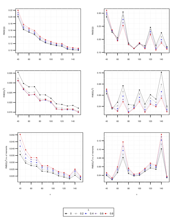
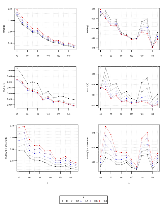
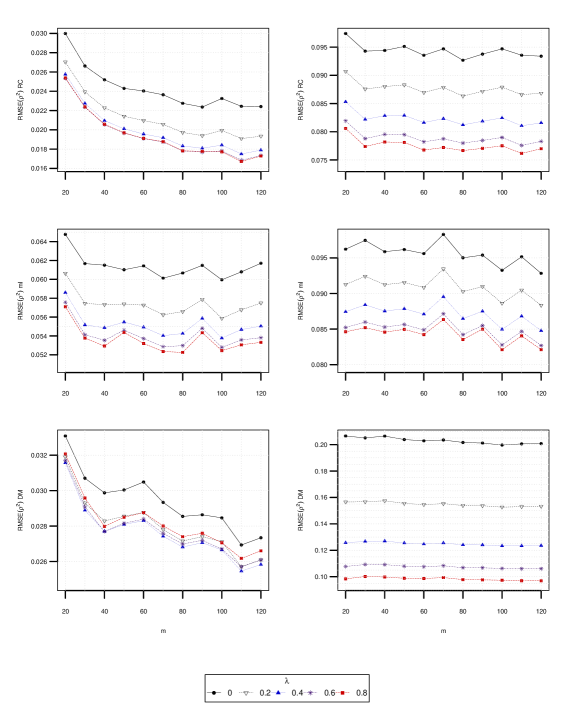
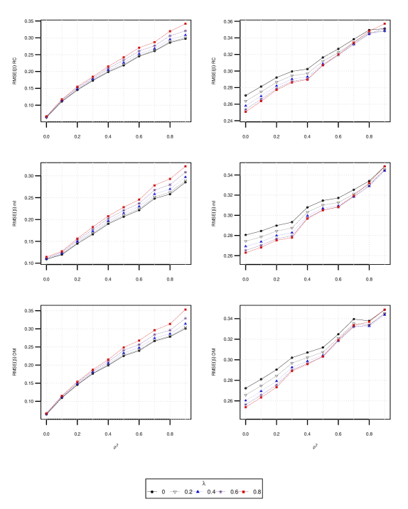
For the above scenarios, we compute the minimum quasi weighted DPD estimator of , for different tuning parameters , and the corresponding estimate of , both for the methods of moments and the estimating equations. The root of the mean square error (RMSE) are then computed based on replications (Figures 5–8).
While classical maximum quasi weighted likelihood estimator presents the best behaviour under pure data, minimum quasi weighted DPD estimators with are much more robust. In particular, as increases, the change on their behaviour is accentuated. This is independent to the sample size (Figures 5 and 6), the intra-cluster correlation and the distribution (Figure 7) considered.
Estimator of by the method of moments seems less precise than the method of estimating equations, with independence of the tuning parameter chosen (Figures 5 and 6). Best estimators of by the estimating equations are obtained from minimum quasi weighted DPD estimators with , both for pure and contaminated data and for any of the distributions considered (Figure 7). Error of the estimators of tends to be smaller with the DM and RC distributions in comparison with the mI distribution, as can be seen in Figure 1, where density plots based on replications are shown for and tuning parameter . These results on the design effect parameter are consistent with the previous work of Alonso et al. (2017).

Notice that estimates are obtained through procedure with tolerance in the software R, used for the whole Monte Carlo study. In Figure 1 iterations needed to compute the corresponding minimum quasi weighted DPD estimators were also obtained, with not a significant difference among the different distributions.

7.3 Comparison of minimum quasi weighted DPD estimators with pseudo minimum phi-divergence estimators
In the previous Section we have illustrated how the quasi minimum quasi weighted DPD estimators present a much more robust behavior than the maximum quasi weighted likelihood estimator for the estimation of when a moderate/large sample size was considered. In Castilla et al. (2018), another family of estimators, the pseudo minimum phi-divergence estimators, was defined in the PLR model with complex survey. In particular, pseudo minimum Cressie-Read divergence estimators for positive tuning parameter were studied. Results of the simulation study suggested these estimators as an interesting alternative to maximum quasi weighted likelihood estimator in terms of efficiency when a small sample size and a large intra cluster correlation was considered. Nevertheless, the robustness of these estimators was not studied.
In this section we want to make a general empirical comparison between minimum quasi weighted DPD estimator and pseudo minimum phi-divergence estimators (with positive and negative tuning parameters in the Cressie-Read subfamily) of , in terms of efficiency and robustness. Although they were not studied in the cited paper of Castilla et al. (2018), phi-divergences with negative tuning parameter and, in particular, the Hellinger distance (), are known to have good robustness properties in some models. See for example Beran (1977) Lindsay (1994) and Toma (2007). This seems to happen in the context of PLR model with complex survey too, when a moderate/large sample size is considered. Nevertheless, pseudo minimum phi-divergence estimators with positive tuning parameter present an important lack of robustness. This behaviour can be summarized in Figure 2.
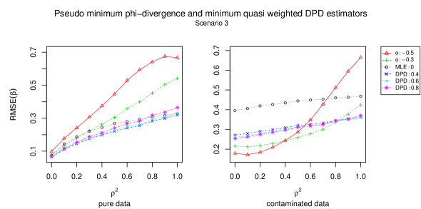
Let us now consider Scenario 3 of the previous section. A comparison between quasi minimum quasi weighted DPD estimators with , classical maximum quasi weighted likelihood estimator, and pseudo minimum phi-divergence estimators with is made. Hellinger distance is shown to be, by far, the best choice when a contaminated scheme with low intra-cluster correlation is considered. With medium/high intra-correlation the behaviour turns to be the opposite. Minimum quasi weighted DPD estimators present a more stable behaviour, both in pure and contaminated schemes, with independence to the correlation parameter.
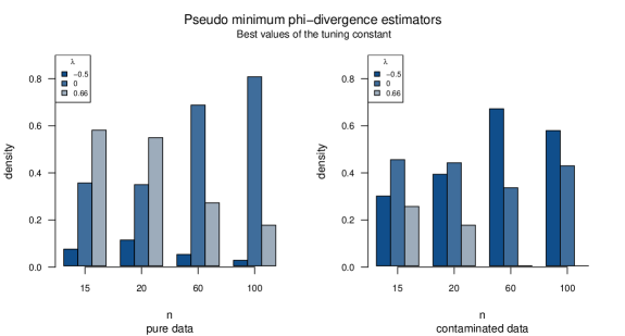
The same divergences are considered now in Scenario 1 for the estimation of the parameter . The estimation of with pseudo minimum phi-divergence estimators is made by the method of Binder (Castilla et al., 2018) while the estimation of with minimum quasi weighted DPD estimators is made by the method of the estimating equations. Pseudo minimum phi-divergence estimators with negative tuning parameter are not competitive neither in the pure nor in the contaminated schemes. Pseudo minimum phi-divergence estimator with tuning parameter is a good alternative to the minimum quasi weighted DPD estimators in contaminated data. This estimator showed also a good behaviour in the paper of Castilla et al. (2018).

7.4 Performance of the Wald-type tests
With the same model as in Section 7.1 we now empirically study the robustness of the minimum quasi weighted DPD estimator based Wald-type tests for the PLR model. As in Castilla et al. (2018) we first study the level under the true null hypothesis . For studying the power robustness, the true data generating parameter value is considered as .
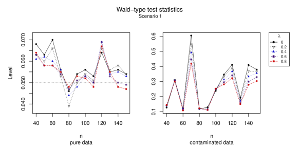
Under Scenario 1, and both for pure and contaminated data, we compute observed levels and powers (measured as the proportion of test statistics exceeding the corresponding chi-square critical value), as can be seen in Figure 4. Under pure data, all levels present a very similar behaviour, while power attains their best value for classical maximum quasi weighted likelihood estimator. Under contamination, minimum quasi weighted DPD estimator based Wald-type tests for present a more robust behaviour than maximum quasi weighted likelihood estimator, in concordance with previous results.
8 Concluding Remarks
We have presented minimum quasi weighted DPD estimators, as a robust alternative to classical approaches, in the modeling of categorical responses with associated covariates through polytomous logistic regression models. A Wald-type family of tests based on these estimators is also presented, for the problem of testing linear hypotheses on regression coefficients. The robustness of both estimators and tests are theoretically justified in terms of the influence function, which is shown to be bounded for the new procedures. An extensive simulation study is also provided, to empirically illustrate their robustness along with a comparison with the pseudo minimum phi-divergence estimators of Castilla et al. (2018). The results clearly show how the proposed minimum quasi weighted DPD estimators seem to be the best choice for dealing with the robustness issue for a moderate sample size.
Appendix A Appendix
Derivation of (10) from (9)
Proof of Theorem 2
Proof. The minimum quasi weighted DPD estimator of , is defined as
which can also be obtained by solving the system of equations where
Now, taking into account that
we get
| (39) |
and hence the system of equations becomes
Proof of Theorem 3
Proof. By following formulas (3.3) and (3.4) of Ghosh and Basu (2013), it holds
which can be expressed as a limit of
where the summands given in (14) and (15) are
With respect to , the first summand estimated from the sample is
and the second one
for , since from . On the other hand,
With respect to , estimated from the sample is given by
where the third equality is again true for . The derivations are omitted for , in which case similar ideas as might be followed.
Proof of Theorem 14
Proof. We have
Now we are going to get the asymptotic distribution of the random variable .
It is clear that and have the same asymptotic distribution because A first Taylor expansion of at around gives
Therefore,
being
Proof of Corollary 4
Proof. It is based on the weak consistency of as well as in the continuity with respect to of the elements of different matrices. Based on Theorem 3,
it holds and and hence .
Proof of Theorem 6
Proof. Let
be another possible consistent estimator of , alternative to . Since
and , for being , for all according to the PLR model with complex design, it holds
is another possible consistent estimator of , alternative to .
Proof of Corollary 7
Proof. Section a) is straightforward considering the expressions of matrix and the related ones. For section b) we consider the vector
Taking into account that we have
for and . An unbiased estimator of is
i.e. for which the trace is
Since is consistent of , it holds that is consistent of , but
is in principle different in shape in comparison with (22) with
where . To assure that both expressions are equivalent we count with the result related to invariance of quadratic forms with generalized variances, Lemma 1a, of Moore (1977), from which is concluded that
Proof of Theorem 8
Proof. The details are omitted for being very similar to Theorem 3 conditioning within each stratum, i.e.
Proof of Theorem 16
Proof. We have
Therefore,
We know, under that
and
The Wald-type test statistics can be written as the quadratic form with
and
where is the identity matrix. The application of the previous gives i). The noncentrality parameter is Result ii) follows using relation (29).
References
- [1] Agresti, A. (2002). Categorical Data Analysis (Second Edition). John Wiley & Sons.
- [2] Alonso-Revenga, J. M., Martín, N. and Pardo, L. (2017). New improved estimators for overdispersion in models with clustered multinomial data and unequal cluster sizes, Statistics and Computing 27, 193-217.
- [3] Basu, A., Harris, I. R., Hjort, N. L. and Jones, M. C. (1998). Robust and efficient estimation by minimizing a density power divergence. Biometrika, 85, 549–559
- [4] Basu, A. Ghosh, A. Mandal, N. Martin and L. Pardo (2017). A Wald-type test statistic for testing linear hypothesis in logistic regression models based on minimum density power divergence estimator. Electon. J. Stat., 11, 2741–2772
- [5] Basu, A. Ghosh, A., Martin and L. Pardo (2018). Robust Wald-type tests for non-homogeneous observations based on the minimum density power divergence estimator. Metrika, 81(5), 493–522.
- [6] Beran, Rudolf (1977). Minimum Hellinger Distance Estimates for Parametric Models. Ann. Statist. 5, no. 3, 445–463.
- [7] Binder, D. A. (1983). On the variance of asymptotically normal estimators from complex surveys. International Statistical Review, 51, 279–292.
- [8] Castilla, E., Martin, N. and Pardo, L. (2018). Minimum phi-divergence estimators for multinomial logistic regression with complex sample design. Advances in Statistical Analysis, 102, 381–411.
- [9] Castilla, E., Ghosh, A., Martin, N. and Pardo, L. (2019). New robust statistical procedures for polytomous logistic regression models. Biometrics. 74, 1282-1291.
- [10] Engel, J. (1988). Polytomous logistic regression. Statistica Neerlandica, 42, 233–252.
- [11] Ghosh, A., and Basu, A. (2013). Robust estimation for independent non-homogeneous observations using density power divergence with applications to linear regression. Electronic Journal of Statistics, 7, 2420–2456.
- [12] Ghosh, A. and Basu, A. (2015). Robust estimation for non-homogeneous data and the selection of the optimal tuning parameter: the density power divergence approach. Journal of applied statitsics, 42, 2056–2072.
- [13] Ghosh, A., and Basu, A. (2016). Robust Estimation in Generalized Linear Models : The Density Power Divergence Approach. TEST, 25, 269–290.
- [14] Ghosh, A., and Basu, A. (2018). Robust Bounded Influence Tests for Independent but Non-Homogeneous Observations. Statistica Sinica, 28, 1133–1155.
- [15] Gupta, A. K., Kasturiratna, D., Nguyen, T. and Pardo, L. (2006). A new family of BAN estimators for polytomous logistic regression models based on density power divergence measures. Statistical Methods & Applications, 15, 159–176.
- [16] Gupta, A. K.; Nguyen, T.; Pardo, L. (2008). Residuals for polytomous logistic regression models based on density power divergences test statistics. Statistics, 42, 495–514.
- [17] Hampel, F. R., Ronchetti, E., Rousseeuw, P. J., and Stahel W.(1986). Robust Statistics: The Approach Based on Influence Functions. New York, USA: John Wiley & Sons.
- [18] Huber, P. J. (1983). Minimax aspects of bounded-influence regression (with discussion). Journal of the American Statistical Association, 69, 383-393.
- [19] Lesaffre, E.and Albert, A. (1989). Multiple-group logistic regression diagnostic. Applied Statistics, 38, 425–440.
- [20] Lindsay, Bruce G. (1994). Efficiency Versus Robustness: The Case for Minimum Hellinger Distance and Related Methods. Ann. Statist. 22, no. 2, 1081–1114.
- [21] Liu, I. and Agresti, A. (2005). The analysis of ordered categorical data: an overview and a survey of recent developments. With discussion and a rejoinder by the authors. Test, 14, 1–73.
- [22] McCullagh, P. (1980). Regression models for ordinary data. Journal of the Royal Statistical Society-Series B, 42, 109–142.
- [23] Morel, G. (1989). Logistic regression under Complex Survey Designs. Survey Methodology, 15, 203–223.
- [24] Morel, J. G. and Koehler, K. J. (1995). A One‐Step Gauss‐Newton Estimator for Modelling Categorical Data with Extraneous Variation. Journal of the Royal Statistical Society: Series C, 44(2), 187–200.
- [25] Morel, G. and Neerchal, N. K. (2012). Overdispersion Models in SAS. SAS Institute.
- [26] Pardo, L. (2005). Statistical Inference Based on Divergence Measures. Statistics: Texbooks and Monographs. Chapman & Hall/CRC, New York.
- [27] Raim, A. M. , Neerchal, N. K. and Morel, J. G. (2015). Modeling overdispersion in R. Technical Report HPCI-2015-1 UMBCH High Performance Computing Facility, University of Maryland, Baltimore Country.
- [28] Roberts, G., Rao, J.N.K. and Kumer, S. (1987). Logistic Regression Analysis of Sample Survey Data, Biometrika, 74, 1–12.
- [29] Toma, A. (2007). Minimum Hellinger distance estimators for some multivariate models: influence functions and breakdown point results. C. R. Acad. Sci. Paris, Ser. I 345, 353–358.
- [30] Warwick, J. and Jones, M. C. (2005). Choosing a robustness tuning parameter. Journal of Statistical Computation and Simulation, 75, 581–588.
- [31] Wedderburn, R. W. M. (1974). Quasi-likelihood functions, generalized linear models, and the Gauss-Newton method. Biometrika, 61, 439–447.