Experimental Comparison of Open Source Visual-Inertial-Based State Estimation Algorithms in the Underwater Domain

Abstract

A plethora of state estimation techniques have appeared in the last decade using visual data, and more recently with added inertial data. Datasets typically used for evaluation include indoor and urban environments, where supporting videos have shown impressive performance. However, such techniques have not been fully evaluated in challenging conditions, such as the marine domain. In this paper, we compare ten recent open-source packages to provide insights on their performance and guidelines on addressing current challenges. Specifically, we selected direct and indirect methods that fuse camera and Inertial Measurement Unit (IMU) data together. Experiments are conducted by testing all packages on datasets collected over the years with underwater robots in our laboratory. All the datasets are made available online.

I INTRODUCTION

An important component of any autonomous robotic system is estimating the robot’s pose and the location of the surrounding obstacles – a process termed Simultaneous Localization and Mapping (SLAM). During the last decade the hardware has dramatically improved, both in performance, as well as cost reduction. As a result, camera sensors and Inertial Measurement Units (IMU) are now mounted in most robotic systems, and in addition to all smart-devices (phones and tablets). With the proliferation of visual inertial devices many researchers have designed novel state estimation algorithms for Visual Odometry (VO) [1, 2] or visual SLAM [3]. In this paper we will examine the performance of several state-of-the-art Visual Inertial State Estimation open-source packages in the underwater domain.

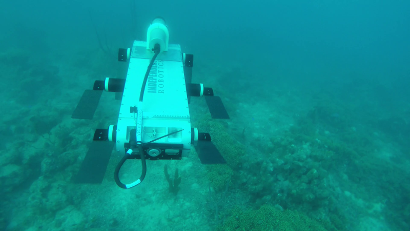
Figure 1: Data collection by an Aqua2 underwater robot [4].

Vision based state estimation algorithms can be classified into a few broad classes. Some methods – such as [5, 6, 7, 8] – are based on feature detection and matching to solve the Structure from Motion (SfM) problem. The poses are estimated solving a minimization problem on the re-projection error that derives from reconstructing the tracked features. Such methods are often termed indirect methods. Direct methods – such as [9, 10] – instead, use pixel intensities directly to minimize the photometric error, skipping the feature detection and matching step.

To improve the state estimation performance, data from other sensors can be fused together with the visual information. Typically, in literature there are two general approaches. One approach is based on filtering, where IMU measurements are used to propagate the state, while visual features are considered in the update phase [11, 12, 13]. The second approach is based on tightly-coupled nonlinear optimization: all sensor states are jointly optimized, minimizing the IMU and the reprojection error terms [14, 15].

Recently, there has been great interest in comparing different approaches, e.g., [16, 17, 18, 19]. However, typically the analysis is limited to only a few packages at a time [16, 19], and rarely to a specific domain [18]. In addition, all these comparisons consider higher quality visual data, not applicable to the underwater domain. In previous work [17], some of the authors compared a good number of state-of-the-art open-source vision-based state estimation packages on several different datasets – including ones collected by marine robots, as the one shown in Figure 1. The results showed that most packages exhibited higher errors in datasets from the marine domain.

This paper considerably expands the previous analysis [17] by selecting ten recent open source packages, focused towards the integration of visual and inertial data, and testing them on new datasets, made publicly available. The contribution of this paper is not in providing a new state estimation method, but in taking a snapshot of the current capabilities of the most recent open-source packages, by evaluating them on datasets collected over the years with underwater robots and sensors deployed by the Autonomous Field Robotics Lab. Such a snapshot allows us to draw some insights on weaknesses, strengths, and failure points of the different methods. A general guideline can be distilled to drive the design of new robust state estimation algorithms.

II Related Work and Methods Evaluated

Visual state estimation methods can be classified according to the following criteria:

• number of cameras, e.g., monocular, stereo, or more rarely multiple cameras;

• the presence of an IMU, where its use could be optional for some methods or mandatory for others;

• direct vs. indirect methods;

• loosely vs. tightly-coupled optimization when multiple sensors are used – e.g., camera and IMU;

• the presence or lack of a loop closing mechanism.

In the following, we provide a brief description of the algorithms evaluated in this paper; please refer to the original papers for in depth coverage. While these algorithms do not cover the exhaustive list of algorithms in the literature, they cover approaches, along the dimensions mentioned above.

LSD-SLAM

Direct Monocular SLAM is a direct method that operates on intensities of images from a monocular camera [9] both for tracking and mapping, allowing dense 3D reconstruction. Validated on custom datasets from TUM, covering indoor and outdoor environments.

DSO

Direct Sparse Odometry [10] is a new direct method proposed after LSD-SLAM by the same group. It probabilistically samples pixels with high gradients to determine the optical flow of the image. DSO minimizes the photometric error over a sliding window. Extensive testing with the TUM monoVO dataset [20] validated the method.

SVO 2.0

Semi-Direct Visual Odometry [21] relies on both a direct method for tracking and triangulating pixels with high image gradients and a feature-based method for jointly optimizing structure and motion. It uses the IMU prior for image alignment and can be generalized to multi-camera systems. The proposed system has been tested in a lab setting with different sensors and robots, as well as the EuRoC [22] and ICL-NUIM [23] datasets.

ORB-SLAM2

ORB-SLAM2 [8] is a monocular/stereo SLAM system, that uses ORB features for tracking, mapping, relocalizing, and loop closing. It was tested in different datasets, including KITTI [24] and EuRoC [22]. The authors extended it to utilize the IMU [15], although, currently, the extended system is not available open source.

REBiVO

Realtime Edge Based Inertial Visual Odometry [25] is specifically designed for Micro Aerial Vehicles (MAV). In particular, it tracks the pose of a robot by fusing data from a monocular camera and an IMU. The approach first processes the images to detect edges to track and map. An EKF is used for estimating the depth.

Monocular MSCKF

An implementation of the original Multi-State Constraint Kalman Filter from Mourikis and Roumeliotis [11] was made available as open source from the GRASP lab [27]. It uses a monocular camera and was tested on the EuRoC dataset [22].

Stereo-MSCKF

Stereo Multi-State Constraint Kalman Filter [28] is also based on MSCKF [11] and was made available from another group of the GRASP lab, while using a stereo camera, and has comparable computational cost as monocular solutions with increased robustness. Experiments in the EuRoC dataset and on a custom dataset collected with a UAV show good performance.

ROVIO

Robust Visual Inertial Odometry [29] employs an Iterated Extended Kalman Filter to tightly fuse IMU data with images from one or multiple cameras. The photometric error is derived from image patches that are used as landmark descriptors and is included as residual for the update step. The EuRoC dataset [22] was used for assessing the performance of the system.

OKVIS

Open Keyframe-based Visual-Inertial SLAM [14] is a tightly-coupled nonlinear optimization method that fuses IMU data and images from one or more cameras. Keyframes are selected according to spacing rather than considering time-successive poses. The optimization is performed over a sliding window and states out of that window are marginalized. Experiments with a custom-made sensor suite validated the proposed approach.

VINS-Mono

VINS-Mono [30] estimates the state of a robot equipped with an IMU and monocular camera. The method is based on a tightly-coupled optimization framework that operates with a sliding window. The system has also loop detection and relocalization mechanisms. Experiments were performed in areas close to the authors’ university and the EuRoC dataset [22].

Table I lists the methods evaluated in this paper and their properties.

TABLE I: Summary of characteristics for evaluated methods.

Method		Camera	IMU	Indirect/	(L)oosely/	Loop
				Direct	(T)ightly	Closure
LSD-SLAM	[9]	mono	no	direct	N/A	yes
DSO	[10]	mono	no	direct	N/A	no
SVO	[21]	multi	optional	semi-direct	N/A	no
ORB-SLAM2	[8]	mono, stereo	no	indirect	N/A	yes
REBiVO	[25]	mono	optional	indirect	L	no
Mono-MSCKF	[27]	mono	yes	indirect	T	no
Stereo-MSCKF	[28]	stereo	yes	indirect	T	no
ROVIO	[29]	multi	yes	direct	T	no
OKVIS	[14]	multi	yes	indirect	T	no
VINS-Mono	[31]	mono	yes	indirect	T	yes

III DATASETS

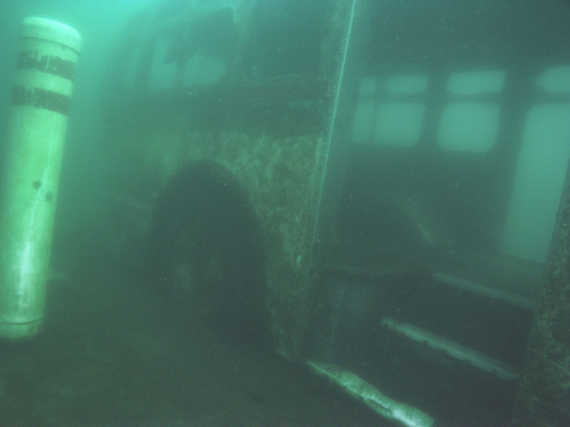
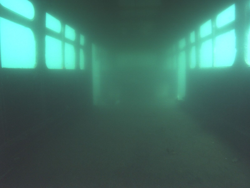
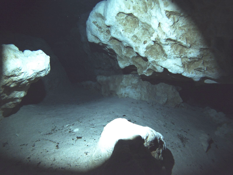
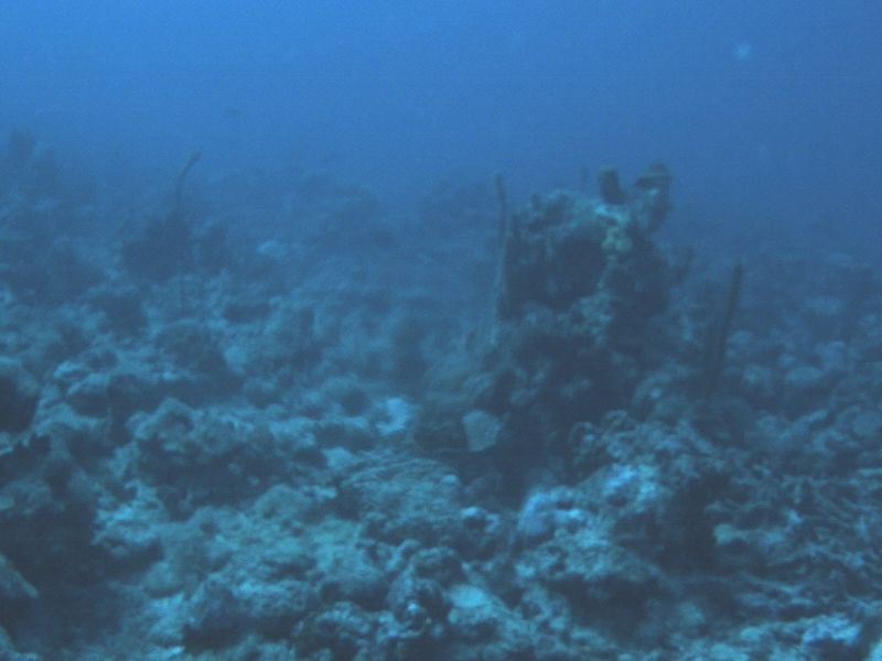
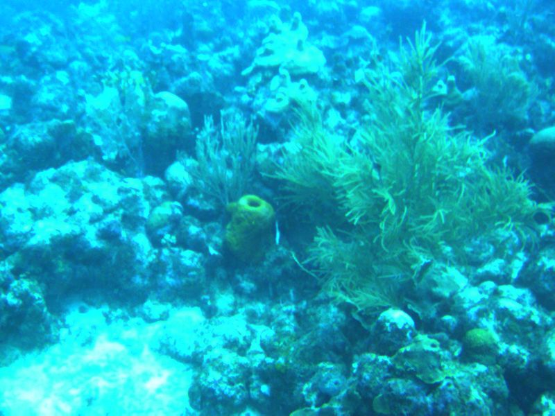
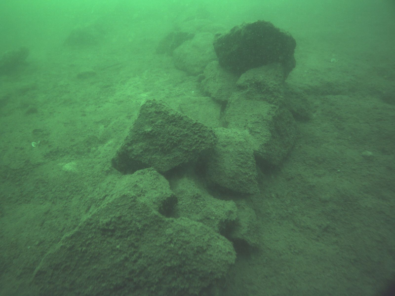
Figure 2: Sample images from the evaluated datasets. (a) UW sensor suite outside a sunken bus (NC); (b) UW sensor suite inside a sunken bus (NC); (c) UW sensor suite inside a cave (FL); (d) UW sensor suite mounted on a Diver Propulsion Vehicle (DPV) over a coral reef; (e) Aqua2 AUV [4] over a coral reef; (f) AUV over a fake cemetery (SC).

Most of the standard benchmark datasets represent only a single scenario, such as a lab space (e.g., [32, 22]), or an urban environment (e.g., Kitti [24]), and with high visual quality. The limited nature of the public datasets is one of the primary motivations to evaluate these packages with datasets collected by our lab over the years in more challenging environments, such as underwater.

In particular, the datasets used can be categorized according to the robotic platform used:

• Underwater sensor suite [33] operated by a diver around a sunken bus (Fantasy Lake, North Carolina) – see Figure 2(a),(b) – and inside an underwater cave (Ginnie Springs, Florida); see Figure 2(c). The custom-made underwater sensor suite is equipped with an IMU operating at $100\text{\,}\mathrm{Hz}$ (MicroStrain 3DM-GX15) and a stereo camera running at 15 fps, $1600\times 1200$ (IDS UI-3251LE); see Figure 3 for operations at Ginnie Springs.

• Underwater sensor suite [33] mounted on an Diver Propulsion Vehicle (DPV); see Figure 4. Data collected over the coral reefs of Barbados; see Figure 2(d).

• Aqua2 Autonomous Underwater Vehicle (AUV) [4] over a coral reef (Figure 2(e)) and an underwater structure (Lake Jocassee, South Carolina) (Figure 2(f)), with the same setup as the underwater sensor suite.

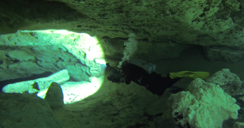
Figure 3: Data collection using a hand-held sonar, stereo, inertial, and depth sensor suite hand-held inside a cavern.

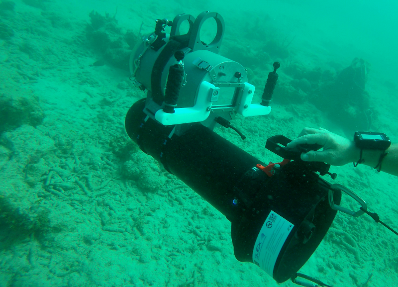
Figure 4: Data collection using a hand-held sonar, stereo, inertial, and depth sensor suite mounted on a DPV. Operations over the coral reefs of Barbados.

Note that the datasets used are more challenging, in terms of visibility, than those used in [17], however the IMU data was collected at a higher frequency – i.e., at least $100\text{\,}\mathrm{Hz}$.

To facilitate portability and benchmarking, the datasets were recorded as ROS bag files and have been made publicly available. The intrinsic and extrinsic calibration parameters for the cameras and the IMU are also provided.

IV Results

IV-A Setup

Experiments were conducted for each dataset on a computer with an Intel i7-7700 CPU @ 3.60GHz, $32\text{\,}\mathrm{GB}$ RAM, running Ubuntu 16.04 and ROS Kinetic. For each sequence in a dataset, we manually set each package parameters, by initializing them to the package’s default values and then by tuning them to improve the performance. This process followed any available suggestion from the authors. Each package was run multiple times and the best performance is reported. For the datasets where ground truth is available, the resulting trajectory is aligned with the ground truth using the sim(3) trajectory alignment according to the method from [34]: the similarity transformation parameters (rotation, translation, and scaling) are computed so that the least mean square error between estimate/ground-truth locations, which are temporally close, is minimized. Note that this alignment might require a temporal interpolation as a pose estimate might not have an exact matching ground truth pose. In particular, bilinear interpolation is used. The resulting metric is the root mean square error (RMSE) for the translation.

Since the datasets used contain stereo images and IMU data, we performed the evaluation of the algorithms considering the following combinations: monocular; monocular with IMU; stereo; and stereo with IMU, based on the modes supported by each VO/VIO algorithm. This not only compares the performance of various VIO algorithms, but also provides insight on how the performance changes as data from different sensors are fused together.

IV-B Evaluation

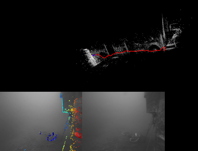
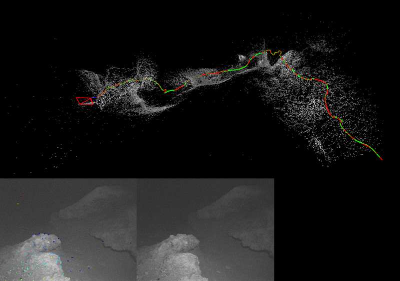
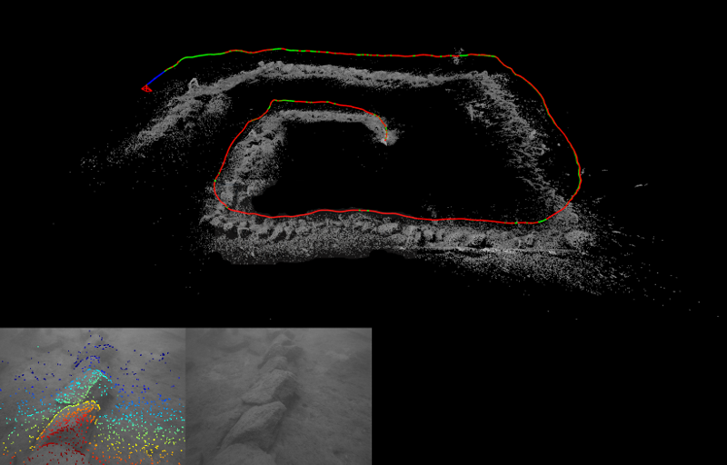
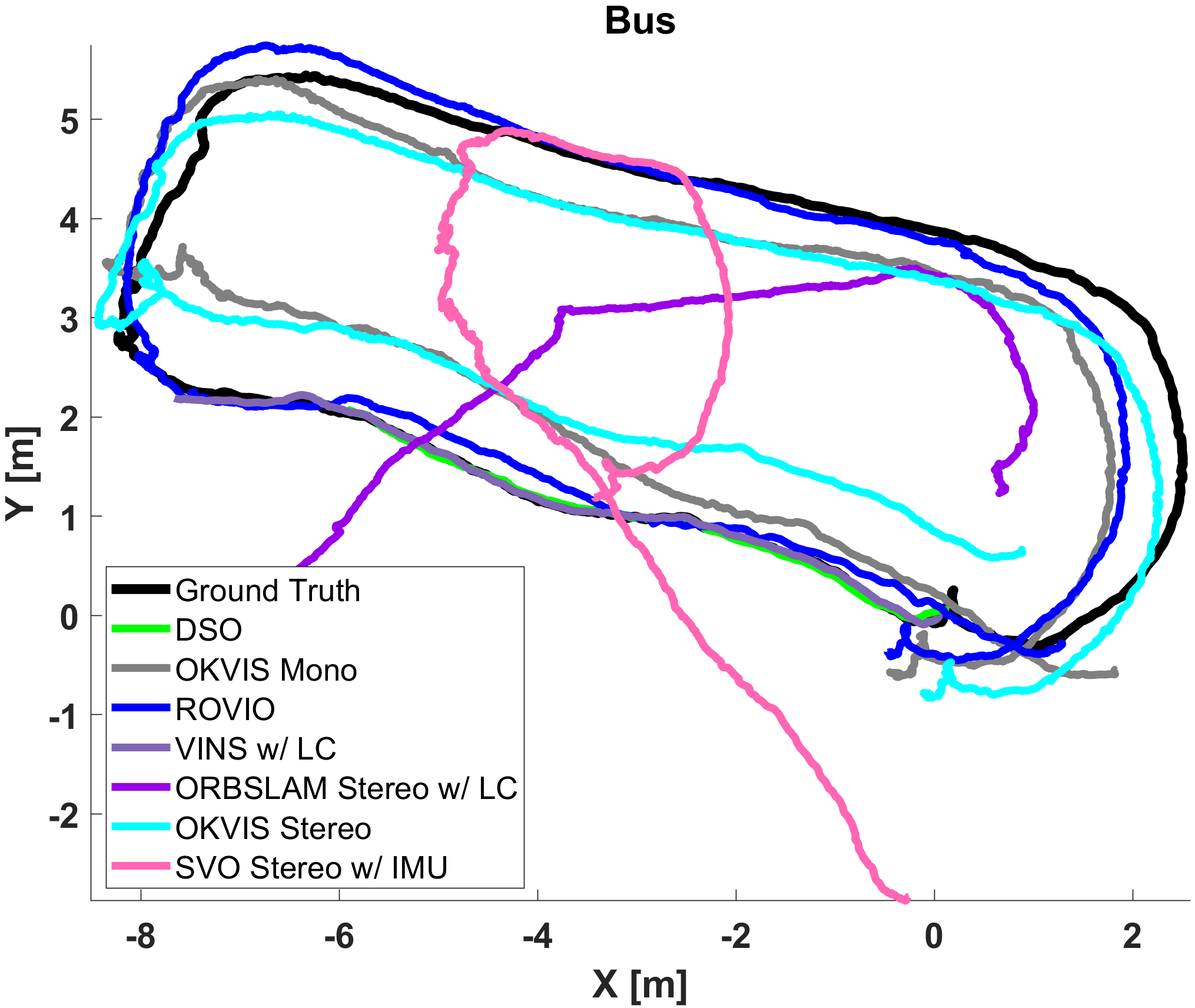
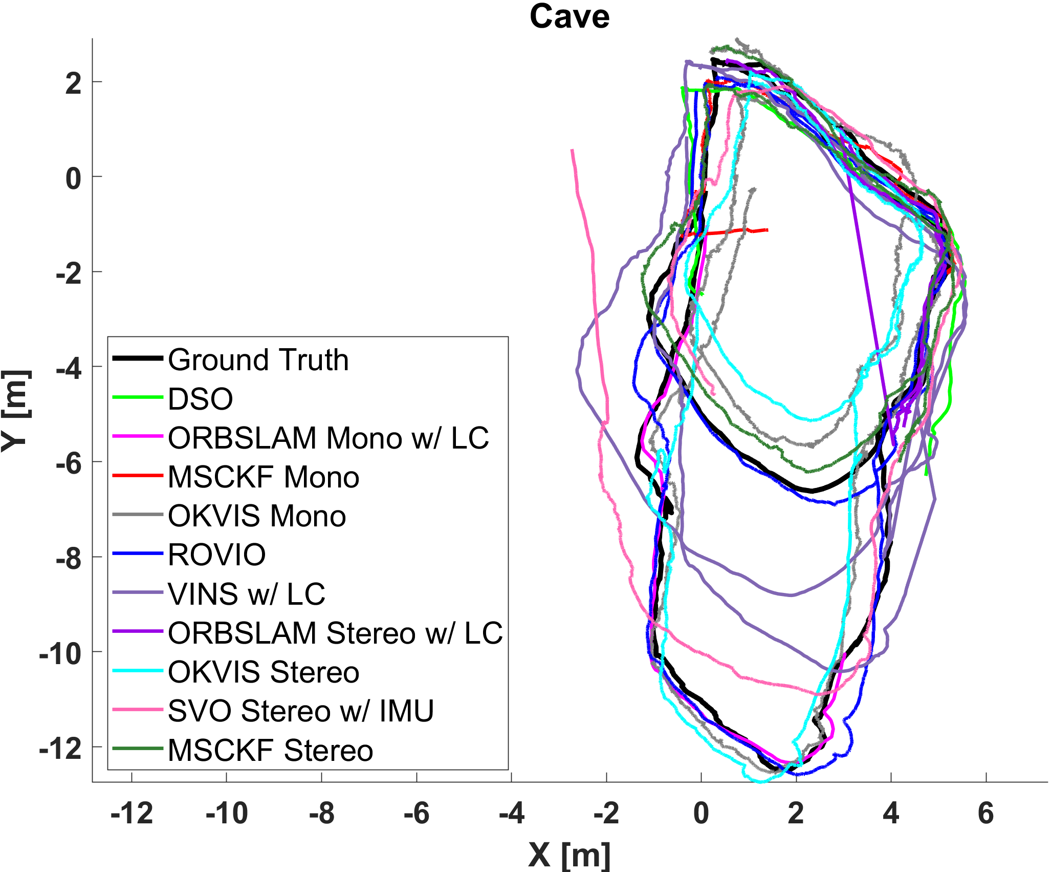
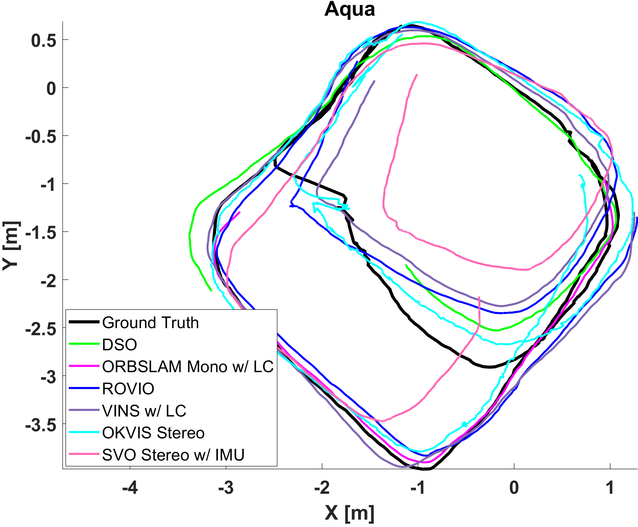
Figure 5: Top row: The partial trajectory and reconstructions from the DSO package for three underwater datasets; outside a sunken bus; inside a cave; AUV over a fake cemetery. Bottom row: sample trajectories for the datasets of the first row.

For the underwater datasets, the work of Rahman et al. [35, 36], which fuses visual, inertial, depth and sonar range data, was used as a reference trajectory given the accurate measurements from the sonar sensor, providing an estimate of the ground truth. In addition, manual measurements between selected points have validated the accuracy of the ground truth measurements used.

For the first four datasets (Bus/In, Bus/Out, Cave, Aqua2Lake) all four (acoustic, visual, inertial, and depth) sensor data were available, together with ground truth measurements. The last two datasets (DPV, Aqua2Reef) had only Visual Inertial and Depth information, and due to the complexity of the trajectory not manual measurements of ground truth. All the datasets provided a major challenge and several packages failed to track the complete trajectory. The best over several attempts was used each time, and the percentage reported indicates what part of the trajectory was completed before the package failed.

ORB-SLAM2 [8] using only one camera (monocular) was able to track the whole trajectory inside the cavern (Cave) and of Aqua2 over the coral reef (Aqua2Reef). Apart from that, pure monocular vision failed to track the whole trajectory in most cases. It is worth noting that DSO, while not able to track the complete trajectory, provided very detailed reconstructions of the environment where it was able to track for a period of time; see Figure 2 top. The addition of IMU brought success to OKVIS, ROVIO, and VINS-Mono (100%), with ROVIO having the best performance, except over the coral reef where it failed due to the lack of features. OKVIS was able to track the complete trajectory in all datasets both in monocular and stereo mode. ORB-SLAM2 with loop closure in stereo mode was also able to track the whole duration on all datasets. SVO was also able to keep track in stereo mode but the resulting trajectory deviates from the ground truth. Stereo-MSCKF was able to keep track most of the time with fairly accurate trajectory. Figure 2 bottom presents the trajectories of several packages together with the ground truth from [36]; all trajectories were transformed to provide the best match.

The overall evaluation of all the experiments can be seen at the bottom rows of Table II. Specifically, we color-coded the qualitative evaluation:

• Green means that the package was able to track at least 90% of the path and the trajectory estimate was fairly accurate with minor deviations.

• Yellow shows that the robot was able to localize for most of the experiment (more than 50%). Also, the resulting trajectory might deviate from the ground truth but overall the shape of the trajectory is maintained. Yellow is also used if the robot tracked the whole sequence, but the resulted trajectory deviates significantly from the ground truth

• Orange is used when a method tracked the robot pose for less than 50% of the trajectory.

• Red marks the pair of package-dataset for which the robot could not initialize or diverges before tracking, or localized less than 10% of the time.

	Monocular			Monocular + IMU						Stereo			Stereo + IMU
	dso	orbslam	orbslamlc	msckf	okvis	rovio	svo	vinsmono	vinsmonolc	orbslam	orbslamlc	svo	okvis	svo	stereomsckf
Bus/Out (53m)	0.04	$\times$	$\times$	$\times$	1.17	0.7	0.19	2.39	2.06	1.78	1.38	2.53	0.78	2.68	0.61
	17%	$\times$	$\times$	$\times$	100%	100%	19%	100%	100%	88%	100%	100%	100%	100%	100%
Cave (97m)	1.56	0.79	0.78	2.42	0.92	0.76	0.79	3.38	1.48	0.58	0.59	3.84	0.98	1.39	0.66
	29%	98%	100%	18%	100%	85%	31%	100%	100%	100%	100%	100%	100%	52%	100%
Aqua2Lake (55m)	0.27	0.64	0.87	$\times$	1.07	0.45	$\times$	0.50	0.50	0.99	0.27	1.61	0.51	1.42	0.51
	23%	52%	57%	$\times$	100%	100%	$\times$	100%	100%	69%	96%	63%	97%	90%	84%
Bus/Out
Cave
Aqua2Lake
Bus/In
DPV
Aqua2Reef

TABLE II: Performance of the different open source packages. Datasets: UW sensor suite outside a sunken bus (Bus/Out); UW sensor suite inside a cave (Cave); Aqua2 (AUV) over a fake cemetery (Aqua2Lake) at Lake Jocassee; UW sensor suite inside a sunken bus (Bus/In); UW sensor suite mounted on a Diver Propulsion Vehicle over a coral reef (DPV); Aqua2 AUV over a coral reef (Aqua2Reef). Quantitative: for each dataset, the first row specifies the RMSE after sim3 trajectory alignment; the second row is the percentage of time the trajectory was tracked; The $\times$ symbol refers to failures. Qualitative: the color chart legend is: red–failure; orange–partial failure; yellow–partial success; green-success.

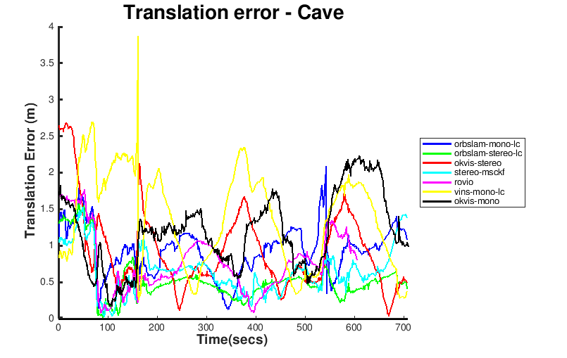
Figure 6: Translation error with respect to time after sim3 alignment for Cave dataset.

Figure 6 shows the absolute translation error over time in the Cave dataset. The error does not monotonously increase because of the loop closure happening at the starting point, reducing thus the accumulated error.

The overall performance of the tested packages is discussed next. LSD-SLAM [9], REBiVO [25], and Monocular SVO were unable to produce any consistent results, as such, they were excluded from Table II.

DSO [10] requires full photometric calibration accounting for the exposure time, lens vignetting and non-linear gamma response function for best performance. Even without photometric calibration, it worked well on areas having high intensity gradients and when subjected to large rotations. In addition, it provided excellent reconstructions; however, in the areas with low gradient images, it was able to spatially track the motion only for a few seconds. Scale change was observed in low gradient images which can be accounted for the incorrect optimization of inverse depth. DSO requires more computational power and memory usage compared to the other packages, which is justifiable since it uses a direct method for visual odometry.

SVO 2.0 [21] was able to track the camera pose over long trajectories, even in parts with few features. It tracks features using the direct method by creating a depth scene. In case of low gradient images, it was subject to depth scale changes, which was predominant in mono camera where tracking failed. SVO in stereo mode without inertial measurements was able to track most of the time but was subject to rotation errors. SVO stereo with IMU was able to keep track most of the time generating a good trajectory estimate.

ORB-SLAM2 [8] (mono) could not initialize in both datasets collected of the sunken bus (Bus/In, Bus/Out). During initialization, it calculates the homography matrix in case of a planar surface and the fundamental matrix from the 8-point algorithm for non-planar 3D structure simultaneously and chooses one of them based on inliers. Since the bus datasets are turbid with low contrast, ORB-SLAM2 cannot find any of the matrices with good certainty and both are rejected. ORB-SLAM2 works fine in the other datasets, but, without loop closure, loses track in some cases. With loop closure, despite track loss, the method can reliably relocalize after the robot traverses a previously seen region.

Mono-MSCKF [27] performed well when the AUV or sensor suite are standing still so that the IMU could properly initialize, otherwise it did not track. Moreover, it was among the most efficient in terms of CPU and memory usage.

ROVIO [29] is one of the most efficient packages tested. Its overall performance was robust on most datasets even when just a few good features were tracked. On the Aqua2Reef dataset though, not enough features were visible and thus it could not track the trajectory.

OKVIS [14] provided good results for both monocular and stereo. In Bus/Out, despite the haze and low-contrast, OKVIS detected good features and tracked them successfully. Also in Cave, it kept track successfully and produced an accurate trajectory even in the presence of low illumination.

VINS-Mono [31] works well in good illumination where there are good features to track. It was one of the few packages that worked successfully in the underwater domain. In the case of Aqua2Reef, it could not detect and track enough features and diverged. With the loop-closure module enabled, VINS-Mono reduced the drift accumulated over time in the pose estimate and produced a globally consistent trajectory.

Stereo-MSCKF [37] uses the Observability Constrained EKF (OC-EKF) [38], which does not heavily depend on an accurate initial estimation. Also, the camera poses in the state vector can be represented with respect to the inertial frame instead of the latest IMU frame so that the uncertainty of the existing camera states in the state vector is not affected by the uncertainty of the latest IMU state during the propagation step. As a result, Stereo-MSCKF can initialize well enough even without a perfect stand still period. It uses the first 200 IMU measurements for initialization and is recommended to not have fast motion during this period. Stereo-MSCKF worked acceptably well in most datasets except Aqua2Reef and DPV. The Stereo-MSCKF could not initialize well over the coral reef due to the fast motion from the start and the low number of feature points. On the DPV dataset, it was able to track only a quarter of the full trajectory before diverging.

V DISCUSSION

Underwater state estimation has many open challenges, including visibility, color attenuation [39], floating particulates, blurriness, varying illumination, and lack of features [40]. Indeed, in some underwater environments, there is a very low visibility that prevents seeing objects that are only a few meters away. This can be observed for example in Bus/Out, where the back of the submerged bus is not clearly visible. Such challenges make underwater localization very challenging, leaving an interesting gap to be investigated in the current state of the art. In addition, light attenuates with depth, with different wavelengths of the ambient light being absorbed very quickly – e.g., the red wavelength is almost completely absorbed at $5\text{\,}\mathrm{m}$. This alters the appearance of the image, which affects feature tracking, even in grayscale.

The appearance of color underwater is different than above, including the color loss with depth. There is a concern when most color shifts to blue, there is a loss of sharpness, which further degrades performance. This will be a venue for further research in the future, in order to investigate the effect of any color restoration to the state estimation process.

From the experimental results it was clear that direct VO approaches are not robust as there are often no discernible features. As such DSO and SVO, quite often fail to track the complete trajectory, however, they had the best reconstructions for the tracked parts. Similar approaches that depend on the existence of a specific feature, such as edges, are not appropriate in underwater environments in general. Overall, as expected, stereo performed better than monocular, the introduction of loop closure enabled the VO/VIO packages to track for longer periods of time, and the introduction of inertial data improved the scale estimations.

One of the most disconcerting findings, which resulted in testing each package multiple times and reporting the best results in this paper, was the inconsistent performance under the same conditions. More specifically, most packages optimize the estimation to achieve frame rate performance, often by restricting the number iterations of RANSAC. While in theory RANSAC converges to the correct solution, in practice, with limited number of iterations allowed, the results vary widely. Most state estimation approaches, historically are tested in recorded data and the performance is presented, however, when relying on the state estimate to follow a trajectory or reach a desired pose, divergence of the estimator will have catastrophic results for the autonomous vehicle. Consequently as the best performance over a number of trials is reported, small variations are not significant.

In the results presented above, the resulting trajectory has been transformed and scaled to produce the best possible estimates. This is acceptable when ground truth is available and the process is off-line, however, if a AUV has to follow a transect for a number of meters or perform a grid search, incorrect scale in the pose estimate will result in failed missions. It is worth noting here that while VINS-Mono produced among the best performances, the scale was always inaccurate; a result of the monocular vision.

For increased robustness and accuracy, the OKVIS and ROVIO gave good performance, ORB-SLAM with loop closure and SVO, for stereo data, and VINS-Mono up to scale also performed well. DSO had the best reconstructions when it was able to track the trajectory.

VI CONCLUSION

In this paper, we compared several open source visual odometry packages, with an emphasis on those that also utilize inertial data. The results confirm the main intuition that incorporating IMU measurements drastically lead to higher performance, in comparison to the pure VO packages, thus extending the results reported in [17]. IMU improved performance was shown across a wide range of different underwater environments – including man-made underwater structure, cavern, coral reef. Furthermore, the study compared popular packages using quantitative and qualitative criteria and offered insights on the performance limits of the different packages. The computational needs for online applications, were qualitative assessed. In conclusion, for the datasets tested, OKVIS, SVO, ROVIO and VINS-Mono exhibited the best performance.

A major concern on integrating these VIO packages in an actual robot for closed-loop control is their non-determinism. In pursuit of higher performance, most packages produce different output for the same input run under the same conditions. Most times the generated trajectory is reasonable, but on occasion tracking is lost and the estimator diverges or outright fails. If an autonomous vehicle was relying on the estimator to complete a mission, it would be hopelessly lost.

Future work will include testing new packages, include new robotic platforms (e.g., BlueROV2), and collecting more challenging datasets with more test cases for each package.

References

- [1] D. Scaramuzza and F. Fraundorfer, “Visual odometry [tutorial],” IEEE Robot. Autom. Mag., vol. 18, no. 4, pp. 80–92, 2011.
- [2] F. Fraundorfer and D. Scaramuzza, “Visual odometry: Part II: Matching, robustness, optimization, and applications,” IEEE Robot. Autom. Mag., vol. 19, no. 2, pp. 78–90, 2012.
- [3] J. Fuentes-Pacheco, J. Ruiz-Ascencio, and J. M. Rendón-Mancha, “Visual simultaneous localization and mapping: A survey,” Artif. Intell. Rev., vol. 43, no. 1, pp. 55–81, 2015.
- [4] G. Dudek, M. Jenkin, C. Prahacs, A. Hogue, J. Sattar, P. Giguere, A. German, H. Liu, S. Saunderson, A. Ripsman, S. Simhon, L. A. Torres-Mendez, E. Milios, P. Zhang, and I. Rekleitis, “A visually guided swimming robot,” in Proc. IROS, Edmonton AB, Canada, Aug. 2005, pp. 1749–1754.
- [5] A. Davison, I. Reid, N. Molton, and O. Stasse, “MonoSLAM: Real-time single camera SLAM,” IEEE Trans. Pattern Anal. Mach. Intell., vol. 29, no. 6, pp. 1052 –1067, 2007.
- [6] A. Geiger, J. Ziegler, and C. Stiller, “StereoScan: Dense 3D Reconstruction in Real-time,” in Intelligent Vehicles Symposium (IV), 2011, pp. 963–968.
- [7] G. Klein and D. Murray, “Parallel tracking and mapping for small ar workspaces,” in IEEE and ACM Int. Symp. on Mixed and Augmented Reality, 2007, pp. 225–234.
- [8] R. Mur-Artal, J. M. M. Montiel, and J. D. Tardós, “ORB-SLAM: A Versatile and Accurate Monocular SLAM System,” IEEE Trans. Robot., vol. 31, no. 5, pp. 1147–1163, 2015.
- [9] J. Engel, T. Schöps, and D. Cremers, “LSD-SLAM: Large-Scale Direct Monocular SLAM,” in Proc. ECCV, 2014, pp. 834–849.
- [10] J. Engel, V. Koltun, and D. Cremers, “Direct sparse odometry,” IEEE Trans. Pattern Anal. Mach. Intell., vol. 40, no. 3, pp. 611–625, 2018.
- [11] A. I. Mourikis and S. I. Roumeliotis, “A multi-state constraint Kalman filter for vision-aided inertial navigation,” in Proc. ICRA, 2007, pp. 3565–3572.
- [12] E. S. Jones and S. Soatto, “Visual-inertial navigation, mapping and localization: A scalable real-time causal approach,” Int. J. Robot. Res., vol. 30, no. 4, pp. 407–430, 2011.
- [13] J. Kelly and G. S. Sukhatme, “Visual-inertial sensor fusion: Localization, mapping and sensor-to-sensor self-calibration,” Int. J. Robot. Res., vol. 30, no. 1, pp. 56–79, 2011.
- [14] S. Leutenegger, S. Lynen, M. Bosse, R. Siegwart, and P. Furgale, “Keyframe-based visual-inertial odometry using nonlinear optimization,” Int. J. Robot. Res., vol. 34, no. 3, pp. 314–334, 2015.
- [15] R. Mur-Artal and J. D. Tardós, “Visual-inertial monocular SLAM with map reuse,” IEEE Robot. Autom. Lett., vol. 2, no. 2, pp. 796–803, 2017.
- [16] B. Williams, M. Cummins, J. Neira, P. Newman, I. Reid, and J. Tardós, “A comparison of loop closing techniques in monocular SLAM,” Robot. Auton. Syst., vol. 57, no. 12, pp. 1188–1197, 2009.
- [17] A. Quattrini Li, A. Coskun, S. M. Doherty, S. Ghasemlou, A. S. Jagtap, M. Modasshir, S. Rahman, A. Singh, M. Xanthidis, J. M. O’Kane, and I. Rekleitis, “Experimental comparison of open source vision based state estimation algorithms,” in Proc. ISER, 2016, pp. 775–786.
- [18] G. Chahine and C. Pradalier, “Survey of monocular SLAM algorithms in natural environments,” in Proc. CRV, 2018.
- [19] J. Delmerico and D. Scaramuzza, “A benchmark comparison of monocular visual-inertial odometry algorithms for flying robots,” in Proc. ICRA, 2018.
- [20] “Monocular visual odometry dataset,” accessed on Feb. 27, 2018. [Online]. Available: https://vision.in.tum.de/data/datasets/mono-dataset
- [21] C. Forster, Z. Zhang, M. Gassner, M. Werlberger, and D. Scaramuzza, “SVO: Semidirect Visual Odometry for Monocular and Multicamera Systems,” IEEE Trans. Robot., vol. 33, no. 2, pp. 249–265, 2017.
- [22] M. Burri, J. Nikolic, P. Gohl, T. Schneider, J. Rehder, S. Omari, M. W. Achtelik, and R. Siegwart, “The EuRoC micro aerial vehicle datasets,” Int. J. Robot. Res., vol. 35, no. 10, pp. 1157–1163, 2016.
- [23] A. Handa, T. Whelan, J. McDonald, and A. Davison, “A benchmark for RGB-D visual odometry, 3D reconstruction and SLAM,” in Proc. ICRA, 2014, pp. 1524–1531.
- [24] A. Geiger, P. Lenz, C. Stiller, and R. Urtasun, “Vision meets Robotics: The KITTI Dataset,” Int. J. Robot. Res., vol. 32, no. 11, pp. 1231–1237, 2013.
- [25] J. J. Tarrio and S. Pedre, “Realtime edge based visual inertial odometry for MAV teleoperation in indoor environments,” J Intell. Robot. Syst., Oct 2017.
- [26] F. Shkurti, I. Rekleitis, M. Scaccia, and G. Dudek, “State estimation of an underwater robot using visual and inertial information,” in Proc. IROS, San Francisco, CA, US, Sep. 2011, pp. 5054–5060.
- [27] Research group of Prof. Kostas Daniilidis, “Monocular MSCKF ROS node,” https://github.com/daniilidis-group/msckf˙mono, 2018.
- [28] K. Sun, K. Mohta, B. Pfrommer, M. Watterson, S. Liu, Y. Mulgaonkar, C. J. Taylor, and V. Kumar, “Robust stereo visual inertial odometry for fast autonomous flight,” IEEE Robot. Autom. Lett., vol. 3, no. 2, pp. 965–972, 2018.
- [29] M. Bloesch, M. Burri, S. Omari, M. Hutter, and R. Siegwart, “Iterated extended Kalman filter based visual-inertial odometry using direct photometric feedback,” Int. J. Robot. Res., vol. 36, pp. 1053–1072, 2017.
- [30] Y. Lin, F. Gao, T. Qin, W. Gao, T. Liu, W. Wu, Z. Yang, and S. Shen, “Autonomous aerial navigation using monocular visual-inertial fusion,” J. Field Robot., vol. 00, pp. 1–29, 2017.
- [31] T. Qin, P. Li, and S. Shen, “VINS-Mono: A robust and versatile monocular visual-inertial state estimator,” IEEE Trans. Robot., vol. 34, no. 4, pp. 1004–1020, 2018.
- [32] J. Sturm, N. Engelhard, F. Endres, W. Burgard, and D. Cremers, “A benchmark for the evaluation of RGB-D SLAM systems,” in Proc. IROS, 2012, pp. 573–580.
- [33] S. Rahman, N. Karapetyan, A. Q. Li, and I. Rekleitis, “A modular sensor suite for underwater reconstruction,” in MTS/IEEE OCEANS - Charleston, 2018, pp. 1–6.
- [34] S. Umeyama, “Least-squares estimation of transformation parameters between two point patterns,” IEEE Trans. Pattern Anal. Mach. Intell., vol. 13, no. 4, pp. 376–380, Apr. 1991.
- [35] S. Rahman, A. Quattrini Li, and I. Rekleitis, “Sonar Visual Inertial SLAM of Underwater Structures,” in Proc. ICRA, 2018, pp. 5190–5196.
- [36] ——, “SVIn2: An Underwater SLAM System using Sonar, Visual, Inertial, and Depth Sensor,” in Proc. IROS, 2019.
- [37] Kumar Robotics, “Robust Stereo Visual Inertial Odometry for Fast Autonomous Flight,” https://github.com/KumarRobotics/msckf˙vio, 2018.
- [38] J. A. Hesch, D. G. Kottas, S. L. Bowman, and S. I. Roumeliotis, “Observability-constrained vision-aided inertial navigation,” University of Minnesota, Dept. of Comp. Sci. & Eng., MARS Lab, Tech. Rep, vol. 1, p. 6, 2012.
- [39] S. Skaff, J. Clark, and I. Rekleitis, “Estimating surface reflectance spectra for underwater color vision,” in British Machine Vision Conference (BMVC), Leeds, U.K., Sep. 2008, pp. 1015–1024.
- [40] K. Oliver, W. Hou, and S. Wang, “Image feature detection and matching in underwater conditions,” in Ocean Sensing and Monitoring II, vol. 7678. International Society for Optics and Photonics, 2010, p. 76780N.