Detailed dust modelling in the L-Galaxies semi-analytic model of galaxy formation

Abstract

We implement a detailed dust model into the L-Galaxies semi-analytical model which includes: injection of dust by type II and type Ia supernovae (SNe) and AGB stars; grain growth in molecular clouds; and destruction due to supernova-induced shocks, star formation, and reheating. Our grain growth model follows the dust content in molecular clouds and the inter-cloud medium separately, and allows growth only on pre-existing dust grains. At early times, this can make a significant difference to the dust growth rate. Above $z\sim 8$, type II SNe are the primary source of dust, whereas below $z\sim 8$, grain growth in molecular clouds dominates, with the total dust content being dominated by the latter below $z\sim 6$. However, the detailed history of galaxy formation is important for determining the dust content of any individual galaxy. We introduce a fit to the dust-to-metal (DTM) ratio as a function of metallicity and age, which can be used to deduce the DTM ratio of galaxies at any redshift. At $z\lesssim 3$, we find a fairly flat mean relation between metallicity and the DTM, and a positive correlation between metallicity and the dust-to-gas (DTG) ratio, in good agreement with the shape and normalisation of the observed relations. We also match the normalisation of the observed stellar mass – dust mass relation over the redshift range of $0-4$, and to the dust mass function at $z=0$. Our results are important in interpreting observations on the dust content of galaxies across cosmic time, particularly so at high redshift.

1 Introduction

Dust has a major impact on the observed properties of galaxies with almost 30% of all photons in the Universe having been reprocessed by dust grains at some point in their lifetime (Bernstein et al., 2002). These grains can form in the stellar winds around AGB and other evolved stars, in supernovae remnants (SNR), and can grow in situ within molecular clouds. Processes that destroy or alter dust grains include shock heating by supernovae, photo-evaporation and chemical explosions (De Boer et al., 1987; Savage & Sembach, 1996). The dust content of a galaxy thus depends in a complex way upon the evolutionary history of its interstellar medium.

The purpose of this paper is to implement a model for dust growth and destruction within the L-Galaxies semi-analytic model in order to investigate the evolution of the dust content of galaxies, with particular regard to the high-redshift Universe.

1.1 Dust production and destruction

The stellar sources of dust are, in order of importance, type II SNR, AGB stars and type Ia SNR. These dust yields are dependent upon the age and metallicity of the stellar populations. For SNR we use the prescription of Zhukovska et al. (2008) and for AGB stars the tables of Ferrarotti & Gail (2006) – this is described in detail in Section 3.1 below. We note that at very high redshifts, $z\gtrsim 6$ observations in the far-infrared have started to identify dust masses substantially in excess of the amount formed from SNR and AGB stars (e.g.  Mancini et al., 2015; da Cunha et al., 2015). It is possible, therefore, that the dust yields may be higher at earlier times, perhaps due to higher survival rates of dust produced in SNR (e.g.  Dwek et al., 2014) – we do not consider that here.

It is now generally accepted that, at later times, the dominant source of dust in the Universe is grain growth inside molecular clouds (e.g.  Mattsson, 2015). Our dust growth model, described in Section 3.2, builds on that of Zhukovska et al. (2008, hereafter ZGT08) and Popping et al. (2017, hereafter PSG17). Unlike earlier works, we use a variable limit for the fraction of an element that can be locked up in dust, motivated by the chemistry of the ISM, and we explicitly follow the dust growth in molecular clouds and the diffuse inter-cloud medium separately, finding that the two can be quite different in certain regimes.

Dust is destroyed by sputtering at high temperatures. In our model, we follow the prescription of McKee (1989) for dust destruction in SNR, described in Section 3.3, and we consider dust to be instantly destroyed if it is reheated out of the cold ISM to join the hot corona of the galaxy. We ignore other processes, such as interaction with cosmic rays, or ejection from the cold ISM by feedback from an active galactic nucleus – we will show in Section 5.3 that we have an excess of dust in massive galaxies at low redshift and this may be one possible cause of that.

1.2 Previous modelling

In recent years, detailed chemical enrichment models have been implemented into both semi-analytic models (SAMs, e.g. Arrigoni et al., 2010; Yates et al., 2013; De Lucia et al., 2014), and hydrodynamical simulations (e.g. Wiersma et al., 2009; Vogelsberger et al., 2013; Pillepich et al., 2018), and a detailed modelling of the dust chemistry is the natural next step. Lately there have been works that incorporated dust models in simulations.

The current efforts of modelling dust in semi-analytic models and hydrodynamic simulations builds heavily upon the initial ‘one-zone’ models, first implemented in Dwek (1998) and followed up by Inoue (2003), Morgan & Edmunds (2003), ZGT08. The most detailed semi-analytic (SA) work, which we use as a basis for our own modelling, is that of PSG17, which uses the SantaCruz (Somerville & Primack, 1999) SA model. Their model was run on a grid of haloes for a range of virial masses with trees created using the extended Press Schechter formalism; whereas our model uses the full set of trees from the relatively low-resolution but cosmologically representative Millennium (Springel et al., 2005a), and the higher-resolution Millennium II (Boylan-Kolchin et al., 2009) simulations (hereafter MR and MRII respectively). Where appropriate, we will make comparison to PSG17 in the results presented below.

Recent studies (e.g. Bekki, 2013; Mancini et al., 2016; McKinnon et al., 2016; McKinnon et al., 2017, 2018; Aoyama et al., 2017; Hirashita et al., 2018; Gjergo et al., 2018; Davé et al., 2019; Hou et al., 2019) have implemented mechanisms for tracking dust production and destruction in hydrodynamical simulations. McKinnon et al. (2016); McKinnon et al. (2017) implemented a simplified dust model in the moving mesh code AREPO to investigate dust formation in a diverse sample of galaxies, accounting for thermal sputtering of grains. Their model gives results in rough agreement at low redshifts for the dust mass function, cosmic dust density and the mean surface density profiles. In McKinnon et al. (2018), the model was improved to track the dynamical motion and grain-size evolution of interstellar dust grains. They predict attenuation curves for galaxies which show large offsets from the observed ones. Aoyama et al. (2017); Hirashita et al. (2018); Hou et al. (2019) considered a simplified model of dust grain size distribution by representing the entire range of grain sizes with large and small grains. They find the assumption of a fixed dust-to-gas (DTG) ratio to break down for galaxies older than 0.2 Gigayears (Gyrs) with grain growth through accretion contributing to a non-linear rise.

1.3 Observational summary

To compare simulations with observational data, it is important to understand how observers calculate the dust properties of their galaxy populations. Derivations of physical dust quantities are generally done using spectral energy distribution (SED) modelling. Many observational studies of dust mass (e.g. Casey et al., 2014; Clemens et al., 2013; Vlahakis et al., 2005) in galaxies fit single or multiple greybodies to galaxy SEDs by assuming an emissivity index, $\beta$ and a dust temperature, T_d, which is quite useful when the available data is limited. More complicated models can also take into account microscopic dust properties, such as the composition and grain size (Zubko et al., 2004). These models also typically assume that the properties and conditions are uniform throughout the galaxy (Rémy-Ruyer et al., 2015), or that the properties in all galaxies at all times are the same as in the local Universe (Santini et al., 2014). For all these reasons, it should be appreciated that measurements of dust mass come with large systematic uncertainties up to a factor of 2-3 (Galliano, F. et al. 2011; Dale et al. 2012).

At higher redshifts, far infrared (FIR), millimetre (mm) and sub-millimetre (sub-mm) observations are generally only possible in extreme galaxies, such as those undergoing starbursts or heavy AGN activity. Sub-mm and mm observations have been shown to be powerful tools in determining how dust and gas are evolving in high-redshift galaxies, with molecular transitions such as CO and the continuum emission used to determine the properties of gas (e.g. Greve et al., 2005; Tacconi et al., 2006; Scott et al., 2011) and dust (e.g. da Cunha et al., 2008) respectively. Sub-mm observations are extremely good at tracing the cold dust component of the galaxy which usually dominates the dust mass. ALMA observations have been instrumental to systematically map the dust continuum (e.g. Hodge et al., 2013; Scoville et al., 2016; Dunlop et al., 2017; Franco et al., 2018) and in some cases, where multi-wavelength data is available, the dust content of galaxies at redshifts of 2–4 (e.g. da Cunha et al., 2015). Further complications arise from the further heating of dust at higher redshifts due to the CMB (da Cunha et al., 2013), and the lack of many observational data points in the FIR means that a dust temperature can not be calculated from the SED and one must be assumed. The assumption of a dust temperature can lead to differing dust masses by up to an order of magnitude (Schaerer et al., 2015).

The observational study of local galaxies by Rémy-Ruyer et al. (2014) found that the dust-to-metal ratio (DTM) is approximately constant in the majority of galaxies. However, at low metallicities, the ratio decreases, suggesting that dust destruction wins out over grain growth. Also at low redshift, De Vis et al. (2019) found that the DTM ratio of DustPedia galaxies (see Davies et al., 2017) increases as galaxies age, before becoming approximately constant once the gas fraction drops below 60 %. For galaxies at higher redshifts ($z>1$), the DTM ratio is seen to increase with metallicity over the broad redshift range of $2\lesssim z\lesssim 5$ (e.g. De Cia et al., 2016; Wiseman et al., 2017), again suggesting that a significant amount of dust is formed due to in situ grain growth in the ISM.

There also have been detections from deep ALMA and PdBI observations of galaxies at extremely high redshifts ($z>6$) with large reservoirs of dust ($>10^{8}\,\mbox{M${}_{\odot}$}$) (e.g. Mortlock et al., 2011; Venemans et al., 2012; Watson et al., 2015; da Cunha et al., 2015). Models to reproduce these (e.g. Michałowski, 2015; Mancini et al., 2015) require either enhanced dust production from supernovae and AGB stars (and reduced destruction by the former), or very rapid dust production soon after chemical enrichment, suggesting very short grain growth timescales in these metal-poor environments. We will look at all these aspects of the dust evolution paradigm in the following sections.

1.4 Structure of the paper

This paper is structured as follows: in Section 2 we describe briefly the L-Galaxies SA model and some of the key ingredients that have been incorporated, including the new two phase-model of cold ISM. In Section 3 we introduce our dust model and describe how it is implemented. We present our results on dust growth in Section 4, and of the dust content of galaxies in Section 5. Finally, we present our conclusions in Section 6.

Throughout this paper we adopt the initial mass function (IMF) of Chabrier (2003), assume the cosmological parameters derived by Planck (Planck Collaboration et al., 2014) and use a solar metallicity value, $Z_{\odot}$ = 0.0134 (Asplund et al., 2009).

2 The Model

Semi analytic models provide a relatively inexpensive method of self-consistently evolving the baryonic components associated with dark matter merger trees, derived from $N$-body simulations or Press-Schechter calculations. The term semi-analytic comes from the use of coupled differential equations to capture the essential galaxy formation physics determining the properties of gas and stars. Most modern SAMs include descriptions of: primordial infall and the impact of an ionizing UV background; radiative cooling of the gas; star formation recipes; metal enrichment; super-massive black hole growth; supernovae and AGN feedback processes; and the impact of the environment and mergers on galaxy morphologies and quenching.

L-Galaxies, (Henriques et al., 2015, and references therein, hereafter HWT15) has been developed over the years to include most of the relevant processes that affect galaxy evolution. In this work we use a modified version of that model which includes: detailed chemical enrichment (Section 2.1); the differentiation of molecular and diffuse atomic phases in the cold gas (see Section 2.2); and the detailed dust model introduced in this paper (see Section 3). We highlight the changes relevant to our dust model below. An overview of all the physics contained within the HWT15 version of the model can be found in the appendix of that paper.

The main non-standard symbols used in our model are:

• $\mu$ – fraction of the cold ISM that is in molecular clouds;

• $f$ – fraction of metals within molecular clouds which condenses into dust;

• $g$ – fraction of metals within the diffuse inter-cloud medium which condenses into dust.

When describing the dust content, we use the following subscripts:

• d – total amount of dust;

• $j$ – elements;

• $x$ – dust species.

2.1 Detailed chemical enrichment

Many galaxy formation models use an instantaneous recycling approximation that assumes that stars pollute their environments with metals the moment they are born. Given the long lifetimes of low-mass stars, this will introduce too many metals (and thus too much dust) at very early times. The detailed chemical enrichment model used here (Yates et al., 2013) only injects metals into the environment at the end of a star’s life. The model takes the metal production rate from stellar mass and metallicity dependent yield tables for type-II supernovae (Portinari et al., 1998), type-Ia supernovae (Thielemann et al., 2003), and AGB stellar winds (Marigo, 2001).

As discussed in Yates et al. (2013), we follow the prescription of Tinsley (1980) for the total rate of metals $j$ ejected by a stellar population at a time $t$:

$$\dot{M}_{j}(t)=\int_{M(t)}^{M_{\rm up}}M_{j}(M,Z_{0})\,\psi(t-\tau_{\rm{M}})\,\phi(M)\,\rm{d}M.$$ (1)

Here $M_{j}(M,Z_{0})$ is the mass of metals released by a star of mass $M$ and initial metallicity $Z_{0}$, $\psi(t-\tau_{\rm{M}})$ is the star formation rate at the time of the star’s birth, and $\phi(M)$ represents the normalised initial mass function (IMF) by number. The lower limit of the integration, $M(t)$, is the mass of a star with a lifetime $t$ (which would be the lowest mass possible to have died by this time), and the upper limit, $M_{\rm up}$, is the highest mass star considered in this work, which is 120M_⊙.

The stellar lifetimes used in the chemical enrichment calculations are taken from the Portinari et al. (1998) mass and metallicity-dependent tables. These provide the lifetime of stars of mass $0.6\leq\rm{M/M}_{\odot}\leq 120$ and for five different metallicities ranging from Z = 0.0004 to 0.05.

With this chemical enrichment model incorporated, L-Galaxies is able to simultaneously reproduce a range of observational data at low redshift, including the mass-metallicity relation for star-forming galaxies, the abundance distributions in the Milky Way stellar disc, the alpha enhancements in the stellar populations of early-type galaxies, and the iron content of the hot intra-cluster medium (see Yates et al. 2013; Yates et al. 2017).

2.2 Molecular gas

The standard L-Galaxies model does not differentiate between atomic and molecular hydrogen in the cold ISM. To model this, we implement the molecular hydrogen prescription used in Fu et al. (2013) to split the cold gas medium into two components - the diffuse ISM and molecular clouds, based on the fitting equations in McKee & Krumholz (2009). In that model, the molecular gas fraction $\mu$ is given by

$$\mu=\begin{cases}\dfrac{4-2s}{4+s},&s<2;\\ 0,&s\geq 2.\end{cases}$$ (2)

The parameter $s$ in Equation 2 is defined as

$$s=\frac{\textnormal{ln}\big{(}1+0.6\chi+0.01\chi^{2}\big{)}}{0.6\tau_{c}}$$ (3)

where $\chi=0.76(1+3.1Z^{{}^{\prime}\,0.365})$ and $\tau_{\textnormal{c}}=0.066\,(\Sigma_{\textnormal{comp}}/\textnormal{M}_{\odot}\textnormal{pc}^{-2})\,Z^{{}^{\prime}}$, with $Z^{{}^{\prime}}=Z_{\textnormal{gas}}/Z_{\odot}$ being the gas-phase metallicity (including metals locked up in dust) relative to the solar value. Also,

$$\Sigma_{\rm{comp}}=c_{\rm{f}}\Sigma_{\rm{gas}}$$ (4)

where $\Sigma_{\textnormal{gas}}=M_{\textnormal{cold}}/\pi r_{\textnormal{d}}^{2}$ is the surface density, $r_{\textnormal{d}}$ is the galaxy disk scale length, and $c_{\rm f}$ is a metallicity-dependent clumping factor given by

$$c_{\rm{f}}=\begin{cases}0.01^{-0.7},&Z^{\prime}\leq 0.01;\\ Z^{{}^{\prime}-0.7},&0.01<Z^{\prime}<1;\\ 1,&Z^{\prime}\geq 1.\end{cases}$$ (5)

which is meant to account for starburst systems in low-metallicity dwarf galaxies.

In our new model, supernovae and stellar winds are assumed to inject a fraction $(1-\mu)$ of their metal and dust into the diffuse component and a fraction $\mu$ into the molecular cloud component. However, star formation and dust growth on grains occurs only in molecular clouds.

We also note that our results remain unchanged on using the molecular hydrogen partitioning recipe used in Martindale et al. (2017) implementing a partitioning based on the mid-plane hydrostatic pressure in the galactic disc from Blitz & Rosolowsky (2006).

3 Detailed dust model

In this section, we describe the new detailed dust model that we have incorporated into L-Galaxies. Our model traces the three dominant sources of dust production in the Universe; injection by type Ia and type II supernovae, stellar winds from AGB stars, and the growth of dust within molecular clouds. We also implement a model of dust destruction induced by supernovae shocks and gas heating. We make the assumption that dust grains only reside within the cold ISM, as the temperature in the hot circumgalactic and intra-cluster media around galaxies is sufficiently high that dust grains will be rapidly destroyed in those gas phases. This is an oversimplification as dust is observed in both the CGM (e.g. Peek et al., 2015) and ICM (e.g. Gutiérrez & López-Corredoira, 2014). Tsai & Mathews (1995) adopted an analytic form for the decrease in the dust grain radius in the hot phase. The sputtering timescale derived from this (used in other studies, e.g. McKinnon et al. 2017; Hirashita et al. 2018) can vary between 1 Myr - 10 Gyr depending on the temperature and the density of the hot phase. Since the sputtering timescales of dust in the hot phase is strongly dependent on the assumed model, we do not consider that here and focus on the dust content of the ISM. This aspect will be revisited in a future work.

The dust production rate of a galaxy is therefore

$$\dot{M}_{\mathrm{d}}(t)=\dot{M}_{\mathrm{d,inj}}+\dot{M}_{\mathrm{d,grown}}-\dot{M}_{\mathrm{d,dest}}-\dot{M}_{\mathrm{d,trans}},$$ (6)

where $\dot{M}_{\mathrm{d,inj}}$ is the dust yield rate from stellar sources (supernovae and AGB stars), $\dot{M}_{\mathrm{d,grown}}$ is rate of dust growth in molecular clouds, $\dot{M}_{\mathrm{d,dest}}$ is the dust destruction rate, and $\dot{M}_{\mathrm{d,trans}}$ is the rate at which dust is transferred out of the cold ISM through processes such as star formation or mergers. We discuss each of these processes in more detail below.

3.1 Supernova and AGB dust yields

By analogy to Equation 1 we have

$$\dot{M}_{\mathrm{d,inj}}=\int_{M(t)}^{M_{\rm up}}M_{\rm{d}}(M,Z_{0})\,\psi(t-\tau_{M})\,\phi(M)\,\mathrm{d}M,$$ (7)

where $M_{\rm{d}}(M,Z_{0})$ is the mass of dust produced by a star of mass M and initial metallicity $Z_{0}$, and the other parameters are as described in Section 2.1. We apply this equation for both AGB winds from lower-mass stars and for supernovae.

The mass of dust produced by a low mass star of given mass and metallicity (i.e. AGB stars) is taken from the tables of Ferrarotti & Gail (2006). In this case, the upper limit of the integral is the maximum possible mass for an AGB star, which is about 8M_⊙.

For supernovae, we follow the prescription laid out in ZGT08. There it is assumed that the mass of dust formed in a supernova remnant is proportional to the total mass return of the key element required to form that particular type of dust. The four types of dust they consider are silicates, carbon, iron, and silicon carbides, where the key element that comprises each species is Si or Mg, C, Fe, and Si, respectively.

We use the following equation to govern the production rate of dust formed by supernovae for the four separate dust species (denoted by a subscript $x$) that we consider:

$$\dot{M}_{x}=\eta_{x}\dot{M}_{j}\frac{A_{x}}{A_{j}},$$ (8)

where $\dot{M}_{j}$ is the mass return rate of the key element, which we obtain from our detailed chemical enrichment model as described in Section 2.1, and $A_{x}$ and $A_{j}$ are the atomic weights of the dust species and key element, respectively. The condensation efficiency parameter, $\eta_{x}$, is used for converting a specific element into dust, as estimated from observations of local supernovae remnants. These efficiency parameters are defined considering the effects of the reverse shock and are therefore smaller than they would be for initial dust condensation.

We apply Equation 8 to all four different dust species for type II supernovae, and for iron-based dust from type Ia supernovae. The values of the parameters that we use are given in Table 1.

Table 1: The conversion efficiencies used for the production of dust grains in supernovae remnants based on the mass return of key metals. The efficiencies have been adopted from ZGT08.

	Dust Species ($x$)
	silicates	carbon	iron	SiC
$\eta_{\rm{x,SNII}}$	0.00035	0.15	0.001	0.0003
$\eta_{\rm{x,SNIA}}$	0.0	0.0	0.005	0.0
$A_{x}$	172.0	12.01	55.85	40.10
	Key Element ($j$)
	Si / Mg	C	Fe	Si
$A_{j}$	121.4 / 24.31	12.01	55.85	28.09

3.2 Grain growth in molecular clouds

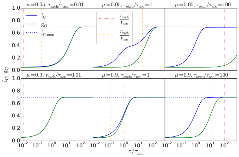
Figure 1: Evolution of the fractions $f_{\mathrm{C}}$ and $g_{\mathrm{C}}$ for different values of $\tau_{\mathrm{exch}}$ and $\mu$ with an initial dust fraction $f_{\mathrm{C}}=g_{\mathrm{C}}=0.05$. These plots are valid for a constant value of $\tau_{\rm{acc}}$, which in our model decreases with the production of more dust, speeding up the saturation of the two fractions. The horizontal dot-dashed line represents the maximum permissible condensation value, fixed here at 0.7 for carbon. The vertical lines show the ratios of the accretion and exchange timescales.

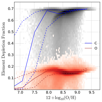
Figure 2: Carbon and oxygen depletion fractions plotted against the total cold-gas metallicity for $z=0$. Blue and brown lines denote the median result from galaxies in our model, with the dashed lines denoting the 84 and 16 percentiles.

A complete model for grain growth would consider how the accretion of different elements varies with different grain sizes, shapes, compositions and grain chemistry, but this would become very complicated. Here, we follow PSG17 in adopting a simpler model in which grain growth inside molecular clouds occurs on a timescale referred to as the accretion timescale ($\tau_{\rm{acc}}$), and exchange of materials between the molecular clouds and the diffuse media is governed by an exchange timescale ($\tau_{\rm{exch}}$) which is also the average lifetime of molecular clouds and is set to 10 Myr (Zhukovska, 2014).

For each element $j$ in the molecular-cloud component of the ISM, we set a maximum condensation fraction that can be locked up in dust, $f_{j,\mathrm{max}}$. There is also an implicit maximum $g_{j}$, which is set by the $f_{j,\mathrm{max}}$ in the molecular clouds. This we fix at unity for the refractory elements Mg, Si, Ca, and Fe, while for N, Ne and S it is set to 0. Neon is unreactive, nitrogen is mostly bound up in volatile gases and sulphur shows little or no incorporation into dust grains (Jones, 2000). In the case of carbon and oxygen, we follow ZGT08 to estimate $f_{j,\mathrm{max}}$. Some carbon is locked up as CO in the molecular clouds and thus not available for grain growth. Observations estimate the fraction of carbon that is locked up as CO inside molecular clouds to be around 20-40 % (Irvine et al., 1987; van Dishoeck & Blake, 1998). In our model we fix this at 30 %, thus setting $f_{\mathrm{C;max}}=0.7$. In the case of oxygen, we assume it is present in dust in the form of metal oxides. Thus, the maximum fraction of available oxygen is set by the amount of other elements present to form these compounds, which are silicates and iron oxides in our model. Following ZGT08, we adopt olivine ([Mg_yFe_1-y]₂SiO₄) and pyroxene (Mg_yFe_1-ySiO₃) as the major silicate compounds in the ISM in the ratio 32:68; here we take $y=0.8$. In the case of iron oxides, we assume hematite (Fe₂O₃) and magnetite (Fe₃O₄) are the major compounds, contributing equally towards dust growth. Thus for oxygen the maximum condensed fraction in molecular clouds depends on the chemical composition.

Grain growth is then implemented by solving the following pair of coupled differential equations at each timestep within the simulation:

$$\frac{\mathrm{d}f_{j}}{\mathrm{d}t}=\frac{f_{j,\mathrm{max}}-f_{j}}{\tau_{\rm{acc}}}+\frac{g_{j}-f_{j}}{\tau_{\rm{exch}}};$$ (9)

$$\frac{\mathrm{d}g_{j}}{\mathrm{d}t}=\frac{f_{j}-g_{j}}{\tau_{\rm{exch}}}\frac{\mu}{1-\mu}=\frac{f_{j}-g_{j}}{\tau_{\rm{exch}}^{\prime}}$$ (10)

where $f_{j}$ and $g_{j}$ are the condensation fractions of element $j$ in dust within the molecular clouds and the diffuse medium, respectively, and $\tau_{\rm{exch}}^{\prime}$ is the effective exchange timescale over which all the ISM in a galaxy is cycled through molecular clouds (see Zhukovska 2014).

Figure 1 shows how the condensation fractions $f_{j}$ and $g_{j}$ evolve for the particular case of carbon. Columns show different $\tau_{\rm{exch}}/\tau_{\rm{acc}}$ ratios, and rows show different molecular gas fractions, $\mu$. For values of $\tau_{\rm{exch}}\ll\tau_{\rm{acc}}$, the condensation fractions evolve similarly for both high and low $\mu$. For $\tau_{\rm{exch}}\gg\tau_{\rm{acc}}$, $f_{\rm C}$ saturates at $f_{\rm{C,max}}$ relatively quickly. However, $g_{\rm C}$ takes a much longer time to reach its maximum allowed value, with its evolution being particularly slow in regions with low $\mu$ (i.e. dominated by diffuse gas).

Because dust catalyses the formation of other dust, we use the following expression for the accretion timescale, which differs from some of the expressions used in previous studies in that it uses the dust mass instead of the metal mass in the denominator:

$$\tau_{\rm{acc}}=\tau_{\rm{acc,0}}\times\bigg{(}\frac{\textrm{Total mass in clouds}}{\textrm{Mass of dust in clouds}}\bigg{)}$$ (11)

We require a short cooling time, $\tau_{\rm{acc,0}}\lesssim 5\times$10⁴ yr to match the high dust masses observed at high redshift, and we adopt this as our canonical value (note that this is lower than the 15 Myr used in PSG17 because of our use of dust fraction rather than metallicity in the growth equation). The impact of varying the value of $\tau_{\rm{acc,0}}$, as well as the evolution of $\tau_{\rm{acc}}$ with redshift, is discussed in Appendix A.

We also show in Figure 2 the depletion fraction i.e. $M_{j,\mathrm{dust}}/(M_{j,\mathrm{cold}}+M_{j,\mathrm{dust}})$ against total gas-phase ISM metallicity in our model for the case of carbon and oxygen. We find that the typical carbon depletion fraction increases over cosmic time, whereas the typical oxygen depletion fraction maintains a value of 0.1 - 0.2 below $z\sim 4$. Our values are comparable to those adopted by emission-line modelling studies (e.g. Groves et al., 2004; Gutkin et al., 2016), and our model reproduces the expectation that oxygen has a relatively low depletion onto dust grains (e.g. Jones, 2000; Jenkins, 2009).

3.3 Dust destruction

We implement a model of dust destruction due to the effects of supernovae induced shock waves following the prescription of McKee (1989):

$$\dot{M}_{d,{\rm dest}}=\frac{M_{\mathrm{d}}}{\tau_{\rm dest}},$$ (12)

where $\tau_{\rm dest}$ is the timescale for destruction of dust.

$$\tau_{\rm dest}=\frac{M_{\rm cold}}{M_{\rm cleared}f_{\rm SN}R_{\rm SN}}$$ (13)

where $M_{\rm cold}$ is the mass of the cold ISM in the galaxy, and $R_{\rm SN}$ the rate of supernovae type II and type Ia going off in the stellar disk, which we directly model. The other two quantities are parameters of the model: $M_{\rm cleared}$ is the amount of cold gas that is totally cleared of dust by an average supernovae which we fix at a lower estimate from Hu et al. (2019) of 1200 M_⊙; $f_{\rm SN}$ accounts for the effects of correlated supernovae and supernovae out of the plane of the galaxy, and is set to 0.36 (McKee, 1989; Zhukovska & Henning, 2013; Lakićević et al., 2015). For a galaxy of similar stellar and cold-gas mass to the Milky Way, this formalism returns a $\tau_{\rm dest}$ in good agreement with the estimates obtained by Hu et al. (2019) for their hydrodynamical simulations of the multiphase ISM in the solar neighbourhood.

We assume that the destruction mechanisms act equally on all types and locations of dust, so that Equation 12 can be applied equally to all dust species. We do not consider dust destruction due to UV radiation, cosmic rays or grain-grain collisions.

3.4 Dust transfer

In this section, we briefly describe the other physical processes within L-Galaxies that act on material within the cold gas phase and thus impact the dust content of galaxies.

3.4.1 Star formation

Stars form from the material present in their birth clouds. We therefore transfer the dust within molecular clouds to the stellar component in proportion to the total mass of stars formed:

$$\dot{M}_{d}=-\frac{M_{\mathrm{d}}}{M_{\mathrm{cloud}}}\dot{M}_{*}$$ (14)

where $M_{\mathrm{d}}$ is the mass of dust within, and $M_{\mathrm{cloud}}$ the total mass of, the molecular clouds, and $\dot{M}_{*}$ is the star formation rate. It should be noted that the star formation prescription is the same as in Henriques et al. (2015).

3.4.2 Mergers

L-Galaxies has separate prescriptions for minor and major mergers. In a major merger, the gas discs of the two progenitor galaxies are assumed to be completely removed through merger-induced star formation and the associated galactic winds driven by supernovae. As we made the assumption that dust can only exist within the ISM, this effectively destroys the dust.

In a minor merger, the disc of the larger galaxy survives and the cold gas component of the smaller galaxy is accreted onto it. In this case, we assume the dust components of the two merging galaxies survive and are placed into the respective disc component of the more massive galaxy.

3.4.3 Other dust destruction mechanisms

There are several other mechanisms, such as reheating or cooling, that transfer dust between different gas phases in a galaxy, such as when supernovae heat up cold gas. Whenever any dust is transferred out of the ISM within our model, we destroy that dust and return it to its metal components. Since we assume dust is completely destroyed in the hot phase, no dust gets transferred from hot to cold phase – this will not significantly alter our results, as there is already a strong equilibrium between the rate of dust production and destruction in the ISM in our current formalism. We direct the reader to the appendix of HWT15 for a complete description of all the processes that affect the gas phases.

4 Results: Dust Growth

In this section, we begin to present some of the results of our model regarding the nature and efficiency of dust growth; in the next section, we will look at the resultant dust content of galaxies. We run the model using the dark matter subhalo trees from the Millennium (hereafter MR, Springel et al. 2005b) and Millennium-II (hereafter MRII, Boylan-Kolchin et al. 2009) N-body simulations of hierarchical structure formation, in order to test our model on a cosmological volume of galaxies, applying a stellar mass selection cut in the respective simulations. Galaxies below/above a stellar mass of 10${}^{9}\mbox{M${}_{\odot}$}$ are selected from from MRII/MR, respectively. The disjoint median lines and hex density on the plots that follow can be attributed to the different volumes of the two simulations. The analysis is restricted to central galaxies (the most massive galaxy inside the halo virial radius), unless stated otherwise.

4.1 Dust-to-Metal (DTM) ratio

The most fundamental diagnostic and test of our model is the dust-to-metal (DTM, M_dust/(M${}_{\rm{metals}}+$M_dust)) ratio which measures the efficiency with which metals are converted in to dust.

4.1.1 DTM versus stellar mass

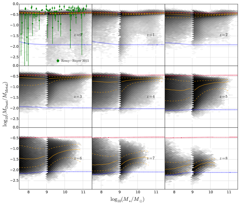
Figure 3: The dust-to-metal ratio as a function of stellar mass from $z=0-8$. The orange line shows the median result from galaxies in our model, with the dashed lines denoting the 84 and 16 percentiles. The red dotted line represents the saturation limit calculated from average metal abundances in the model while the blue dotted line is the median DTM ratio obtained from stellar injection alone. Green points show the observational constraints from Rémy-Ruyer et al. (2015).

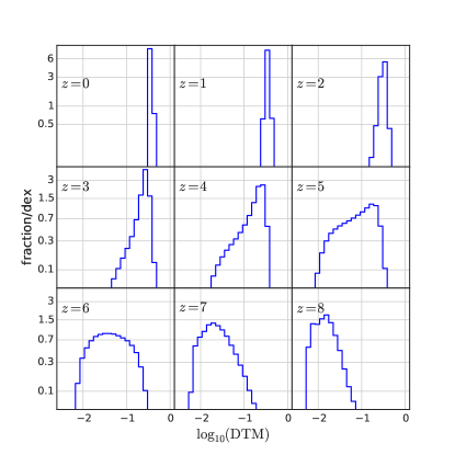
Figure 4: The distribution of DTM ratios for various redshifts from 8 to 0. The peak of the distribution clearly shifts from low to high values over cosmic time.

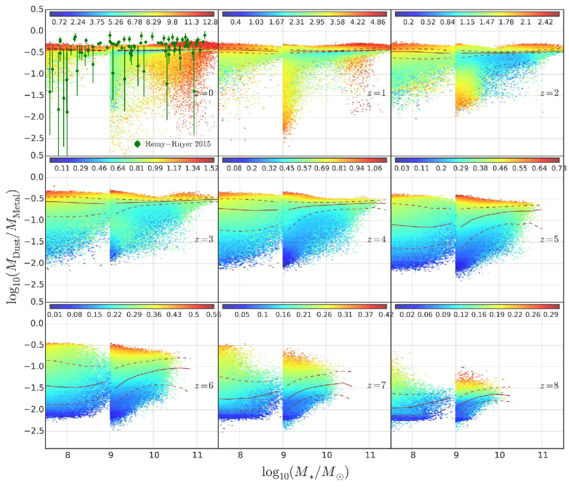
Figure 5: The dust-to-metal ratio as a function of stellar mass from $z=0-8$, same as Figure 3, with galaxies coloured according to their mass-weighted stellar age in Gyrs. Green points show the observational constraints from Rémy-Ruyer et al. (2015).

Figure 3 shows how the DTM ratio varies with stellar mass, with the green coloured observational data points taken from Rémy-Ruyer et al. (2015). The solid line shows the median result of the galaxies in our model, while the dashed lines show the 84 and 16 percentiles. The hex diagram in grey shows a 2D density distribution of galaxies in our model. The dotted, red line in the plot shows the maximum possible DTM ratio in our model (for the median metallicity), assuming that grain growth has saturated (i.e. $f_{j}=f_{\textnormal{{j},max}}$ for every element). The blue dotted line shows the median DTM ratio obtained from stellar dust production mechanisms alone. The slight displacement of the median DTM ratio below the saturation value at low redshift is due to dust destruction mechanisms that offset some of the grain growth; the slight offset of the median DTM ratio above the blue line at high redshift is due to the fact that dust growth takes off very quickly. The transition from galaxies dominated by dust injected by stellar sources (mostly type II SNe) and that dominated by grain growth occurs at $z\sim 6$, as illustrated in Figure 4 which shows the fraction of galaxies in different DTM ratio bins.

The Rémy-Ruyer et al. (2015) data shown in Figure 3 combines two samples of local galaxies from the Herschel: Dwarf Galaxy Survey (DGS Madden et al. 2013, to study low-metallicity systems) and the Key Insights on Nearby Galaxies: a Far-Infrared Survey with Herschel (KINGFISH Kennicutt et al. 2011, mostly spiral galaxies along with several early-type and dwarf galaxies to include metal-rich galaxies). They use a semi-empirical dust SED model presented in Galliano, F. et al. (2011) to derive dust masses and estimate systematic errors of order 2$-$3. The DTM ratio predictions from our model show reasonable agreement with this data, although the dispersion in the model predictions is lower, and some of the highest observed DTM ratios are incompatible with the predictions of our model: the extent to which that is due to observational uncertainty is hard to assess.

The transition from the lower to the upper locus in Figures 3 & 4 is largely a function of the age of the galaxy – grain growth needs time to act (see also Appendix A). This is shown clearly in Figure 5 which plots the same relation with galaxies coloured by their mass-weighted stellar age. Although the precise time taken for grain growth to saturate will depend upon the metallicity and initial dust content of the ISM, it takes of order 1 Gyr to do so. A study by Inoue (2003) has also shown that the evolutionary tracks in the metallicity – DTM ratio plane depends on the star-formation history.

At $z=0$, the DTM ratio in some of the oldest, most massive galaxies has again begun to fall slightly and in some significantly – these are early types for which the molecular gas content of the cold ISM is low. We can therefore see that a galaxy’s DTM ratio depends strongly on it’s age, but also more weakly on it’s chemical enrichment, molecular gas consumption, and other factors relating to its evolutionary history.

If we compare our results to PSG17 (their Figure 6), our model galaxies do not exhibit any evolution of the DTM ratio with stellar mass as seen in their results at $z=0$. But the scatter at $z=0$, is negligible similar to PSG17. At all redshifts their DTM ratio remains almost constant as well as exhibiting negligible scatter below M${}_{*}=10^{8.5}$M_⊙, while increasing rapidly afterwards due to their grain growth mechanism dominating the dust production. The cause of these differences are explained in Section 4.2.

4.1.2 DTM versus metallicity

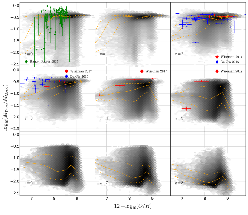
Figure 6: The dust-to-metal ratio as a function of their metallicity from z = 0-8. The orange line shows the median result from galaxies in our model, with the dashed lines denoting the 84 and 16 percentiles. Green blue and red points show the observational constraints from Rémy-Ruyer et al. (2015), De Cia et al. (2016) and Wiseman et al. (2017) respectively.

Figure 6 shows the DTM ratio as a function of the gas-phase ISM oxygen abundance (i.e. the oxygen not locked up in dust). At $z=0$, we again compare to observations from Rémy-Ruyer et al. (2015). We match the normalization of the observations for $12+\log_{10}$(O/H)$>8$ and also some scatter down to low DTM ratios, noting that the low-DTM observational data tend to have the largest uncertainties. At higher redshifts, we show a good fit to the DTM ratios deduced by observations of gamma ray bursts (GRBs Wiseman et al., 2017) and damped lyman-alpha emitters (DLAs De Cia et al., 2016).

At $z\geq 6$ there appears a negative trend in the DTM-metallicity relation with increasing metallicity. This is due to the fact that at these high redshifts grain growth has not had sufficient time to enrich the cold ISM. This trend also emerges from the dust injection tables used in the model, since at these redshifts the DTM ratio follows the stellar injection modes of dust production. The same feature is seen in the model varaints that are discussed in PSG17. The feature is absent in the fiducial model used in PSG17 due to their grain growth mechanism dominating the dust production (see Section 4.2).

4.1.3 DTM fitting function

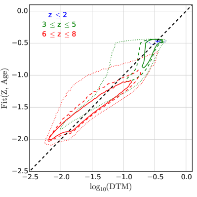
Figure 7: The DTM fitting function in Equation 15 is plotted against the DTM ratio from the model as contour enclosing different percentiles of the data. The blue, green and red contour lines represent model galaxies with $z\leq 2$, $3\leq z\leq 5$ and $6\leq z\leq 8$ respectively. Solid, dashed and dotted lines represent the 50, 68 and 95th percentile respectively. The dashed black line represents the one-to-one relation between the fitting function and the data.

As we have seen, the DTM ratio can vary by a large amount, depending upon the evolutionary history of a galaxy. It would be useful to be able to capture that behaviour with a suitable fitting function. Motivated by our conclusions earlier in this section, we posit the following functional form:

$$\rm{DTM_{\textnormal{fit}}}=\mathcal{D}_{0}+(\mathcal{D}_{1}-\mathcal{D}_{0})\,\big{[}1-exp\big{(}-\alpha\,Z^{\beta}(Age/\tau)^{\gamma}\big{)}\big{]},$$ (15)

where $\mathcal{D}_{0}$ and $\mathcal{D}_{1}$ represent the initial type II SNe dust injection and the saturation value, respectively, $Z$ is the metallicity of the interstellar medium, Age is the mass-weighted age of the stellar population, and $\tau=\tau_{\mathrm{acc,0}}/\mathcal{D}_{0}\,Z$ is an estimate of the initial dust growth timescale after dust injection from type II supernovae but prior to the initiation of dust growth on grains.

Fixing the values of $\mathcal{D}_{0}$ and $\mathcal{D}_{1}$ by reference to Figure 3, the best fit values (using the Levenberg-Marquardt method implemented in the python package scipy.optimize.curve_fit) to the other parameters are:

$$\mathcal{D}_{0} =0.008,$$

$$\mathcal{D}_{1} =0.329,$$

$$\alpha =0.017,$$

$$\beta =-1.337,$$

$$\gamma =2.122.$$

The above fitting function is plotted against the DTM ratio in the model in Figure 7 for $z=0-8$. The majority of galaxies lie close to the fit, well within about a factor of 2, although the full dispersion in DTM ratios is not quite captured. This then provides a good estimate of dust extinction should the metallicity and age of a galaxy be known, and offers a significant improvement upon the fixed DTM ratios often assumed in the literature (e.g. Wilkins et al., 2017). We show in the appendix that the same fitting function holds good for different choices of $\tau_{\mathrm{acc,0}}$.

4.2 Integrated dust production rates

Figure 8: The production rate of dust through different mechanisms as a function of redshift for the MR run. Red, blue and yellow lines show the contribution from stellar sources of dust production, type II supernovae (SNII), AGB stars and type Ia supernovae (SNIA) respectively. The green line (largely obscured) shows the contribution from grain growth (GG) inside molecular clouds. The black line shows the dust destruction rate (DEST). The orange line shows the net total dust production rate (NET), taking into account all production and destruction. We also plot the star formation rate (SFR) density as a dashed cyan line for comparison.

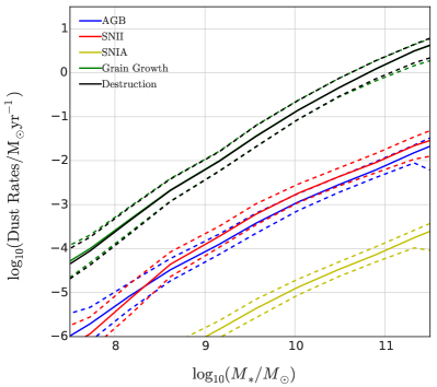
Figure 9: The production rate of different dust mechanisms as a function of stellar mass, shown for $z=0$. Blue, red and yellow lines show the median contribution from stellar sources of dust production: AGB stars, type II supernovae and type Ia supernovae respectively, with the dashed lines denoting the 84 and 16 percentiles. The green line shows the contribution from grain growth inside molecular clouds. The black line shows the dust destruction rate.

The detailed dust model we have built includes several different dust production and destruction mechanisms that all contribute to the final dust properties of the galaxies in our model. Figure 8 shows the mean dust production (or destruction) rate densities as a function of redshift for galaxies in the (480 $h^{-1}$Mpc)³ MR simulation. The total dust destruction rate plotted includes destruction from supernovae, star formation, and reheating. We also plot the star formation rate density for comparison.

We can see that grain growth in molecular clouds dominates the production of dust over the redshift range $z=0-8$, rapidly increasing towards its peak at $z=2$. The destruction rate closely follows the dominant grain growth production rate, suggesting that any dust destroyed is rapidly recycled by grain growth. While at very early times type II supernovae dominate the production of dust. Thus, at the highest redshifts, the dispersion in the DTM ratio is small, with the dispersion increasing rapidly as grain growth takes over at $z<8$.

If we look at the stellar contributions to the dust content, we see that type II supernovae are the dominant stellar production mechanism across the whole redshift range, peaking at $z\sim 2$, closely following the shape of the star formation rate as one would expect. Dust production (and metal enrichment) from Type Ia supernovae is shifted to slightly later times, due to the power-law delay-time distribution (DTD) we assume, which allows $\sim{}52$ per cent of the supernovae to explode $>400$ Myr after star formation (see Yates et al. 2013). Nonetheless, Type Ia supernovae never have a significant impact on the dust production rate. It is worthwhile to note that many other works also suggest that Type Ia supernovae are unlikely to be the major sources of ISM dust (e.g. Nozawa et al., 2011). Production by AGB stars is also negligible at early times, but rises at late times to rates approaching that of type IIs.

It is important to note that, although grain growth is the dominant dust formation mechanism at all redshifts below $z=8$ when averaged over the whole galaxy population, the dust content of individual galaxies can vary enormously. At $z=6$, for example, grain growth exceeds stellar dust injection by a factor of 6, but the spread in DTM ratios seen in Figure 4 extends over more than a decade.

The variation of the dust production rates with stellar mass is shown in Figure 9 for $z=0$ for star forming galaxies (defined here as galaxies with a specific star formation rate, sSFR $>1/3t_{\rm{H}}(z)$, where $t_{\rm{H}}(z)$ is the age of the Universe at redshift z). From this it is clear that there is very little dependence of dust growth and destruction upon galaxy mass. The same holds too at all other redshifts.

If we compare our dust production rates with the PSG17 model (their Figures 8 & 10), this is bound to be different since the models differ in the grain growth implementation as well as the dust yield tables used for stellar production mechanisms. But the trends seen in both the models are similar in the sense that grain growth dominates over all the other production mechanisms at almost all redshifts from z = 0-8. In their model, the median grain growth rate is approximately 3 orders of magnitude higher than any stellar production mechanisms for high stellar mass ($>10^{10}M_{\odot}$) at all redshifts. In our model, the dust production rate from SNII and grain growth is similar at z $\sim$ 8. Also, we note that the production rates for each of the various sources (SNe-II, AGB stars, and grain growth) are similar between the two models at high mass, whereas they are three to four orders of magnitude greater at low mass in our model compared to PSG17. These differences in the dust production rates from different processes are reflected in slight differences seen in our results for the dust content of galaxies, discussed in the next section.

5 Results: Dust content of galaxies

In this section we compare the predicted dust content of galaxies in our model to observations such as the dust-to-gas ratio, the stellar-mass – dust-mass relation and the dust mass function.

5.1 Dust-to-Gas (DTG) ratio

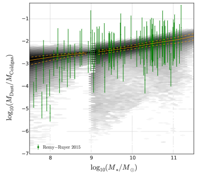
Figure 10: The dust-to-gas ratio as a function of stellar mass for z = 0. The orange line shows the median result from galaxies in our model, with the dashed lines denoting the 84 and 16 percentiles. Green points show the observational constraints from Rémy-Ruyer et al. (2015).

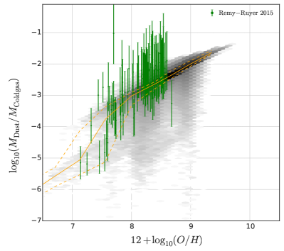
Figure 11: The dust-to-gas ratio as a function of gas phase metallicity for z = 0. The orange line shows the median result from galaxies in our model, with the dashed lines denoting the 84 and 16 percentiles. Green points show the observational constraints from Rémy-Ruyer et al. (2015).

We compare the DTG ratio to two different properties, first, to see how the DTG ratio varies with stellar mass in Figure 10, and secondly how it varies with oxygen abundance, as seen in Figure 11. Because of the difficulty in obtaining observational data for comparison, we show only results for $z=0$; at higher redshifts, the DTG ratio exhibits the same behaviour seen for the DTM ratio in Figure 3.

In Figure 10, we compare the DTG ratio of our model versus stellar mass against observations from Rémy-Ruyer et al. (2015). The median value of our model fits the observations well, particularly above stellar masses of $10^{8}$M_⊙. Below this value, there may be a downturn in the DTG ratio in the data, that we do not see. Figure 11 shows the same data plotted as a function of oxygen abundance and here we see that the low DTG ratios are associated with low metal abundance, and that the observations and the model overlap quite well. The reason for the discrepancy seen at low masses in Figure 10 is therefore due to the fact that our low-mass galaxies mostly have higher oxygen abundance than those in the Rémy-Ruyer et al. (2015) sample.

The PSG17 (their Figure 4 and 3) as well as Hou et al. (2019) (their Figure 4a and 4b) model exhibits a similar trend to our predictions when the DTG ratio is plotted as a function of stellar mass and metallicity respectively. But at all redshifts both the models exhibits a steeper slope, such that their lower mass model galaxies have lower DTG ratios. In case of McKinnon et al. (2017), the DTG ratio shows a flat trend with metallicity (their Figure 8) for 12 + log(O/H) > 8 while showing a positive correlation below that.

5.2 Dust versus stellar mass

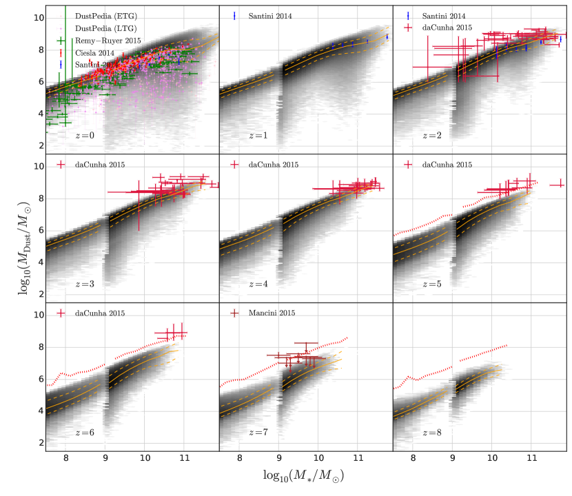
Figure 12: The stellar-dust mass relation for redshifts $z=0-8$. The orange line shows the median result from galaxies in our model, with the dashed lines denoting the 84 and 16 percentiles. Pink, violet, red, green, blue, crimson and brown points show the observational constraints from the DustPedia archive (see Davies et al., 2017, separated into ETGs and LTGs), Ciesla et al. (2014), Rémy-Ruyer et al. (2015), Santini et al. (2014), da Cunha et al. (2015) and Mancini et al. (2015) respectively. At redshifts 5 and above, the dotted red line shows the maximal dust content that could be predicted by our model, assuming saturated grain growth and no dust destruction.

The dust mass versus stellar mass relation is shown in Figure 12. The evolution in dust masses mimics that shown in Figure 3 for the DTM ratio. At $z=0$ most of the galaxies have saturated dust growth on grains. This persists up to $z=4$, after which there is a gradual transition down to the levels expected for dust injection from stellar sources.

The stellar-dust mass parameter space is one where we have observational constraints across a very large range of redshifts. The coloured points in Figure 12 represent observations from a number of different studies (DustPedia collaboration Davies et al., 2017; Ciesla et al., 2014; da Cunha et al., 2015; Mancini et al., 2015; Rémy-Ruyer et al., 2015; Santini et al., 2014). The DustPedia data combine the Herschel/Planck observations with that from other sources of data, and provide observations at numerous wavelengths across the spectral energy distribution. The dust masses are fitted using CIGALE assuming either the dust model from Draine et al. (2014) or their own called THEMIS (see Davies et al. 2017). We use the dust masses fitted by the former model, since the latter has a lower normalisation at $z=0$ compared to our dust masses. The Ciesla et al. (2014) data uses the Herschel Reference Survey (Boselli et al., 2010), where the dust masses are obtained using the SED templates described in Draine & Li (2007). da Cunha et al. (2015) derives dust masses from a sample of sub-mm galaxies in the Alma LESS survey using the SED fitting techniques described in da Cunha et al. (2008). Some of the galaxies in the sample only have photometric redshifts and thus the redshift is kept as a free parameter in their fitting technique. Mancini et al. (2015) uses ALMA and PdBI observations with upper limits on the dust continuum emission. They derive the stellar masses using the mean relation between the UV magnitude and the dust mass assuming T_d = 35K and $\beta$ = 1.5. Santini et al. (2014) uses galaxies in the GOODS-S and GOODS-N field as well as the COSMOS field which have FIR observations carried out using Herschel. They also use the SED templates of Draine & Li (2007) as a description for their dust masses.

The first thing to note is that there is a significant offset in normalisation between the different observational data sets at $z=0$. Thus we see that, while the median dust content predicted by our model is consistent with the LTGs from DustPedia and Ciesla et al. (2014) data, it lies well above that of Rémy-Ruyer et al. (2015) and Santini et al. (2014). This reflects the different observational biases and systematic uncertainties in the estimation of dust content. For example, the Rémy-Ruyer et al. (2015) sample contains some massive AGN-host galaxies which are presumably older and have low gas fractions, leading to smaller dust masses. Also a part of their sample (DGS, Madden et al., 2013) was chosen to study low-metallicity environments and hence exhibit smaller dust masses.

Although the median dust level is acceptable, it would appear that we have many galaxies, particularly at masses above about 10¹⁰ M_⊙, whose dust content is significantly higher than those seen in the observational samples considered here. This could come about in one of three ways: too much cold gas; too high a metallicity in the cold gas; too high a dust-to-metal (DTM) ratio. The cold gas content of galaxies in the HWT15 model was considered in Martindale et al. (2017) and while the Hi mass function was in good agreement with the observations, the gas-to-stellar mass ratio is, if anything, slightly too low (although the selection functions for the Hi surveys are hard to reproduce). Similarly, Yates et al. (2013) showed that the oxygen abundance of cold gas in our model is in good agreement with observations from SDSS. Finally, Section 4.1 of this paper shows that the DTM ratio is in good agreement with that of Rémy-Ruyer et al. (2015). It is thus slightly perplexing that we seem to have these galaxies with excessive dust. We note that in our model, we have ignored possible dust destruction due to the effects of cosmic rays, photoevaporation or AGN activity that start to play a major role in high mass galaxies.

There is also a significant spread in observed dust masses to lower values at high stellar masses at $z=0$ due to the presence of elliptical early-type galaxies (ETGs) with low molecular gas content. We predict many such galaxies in our model (see also Figure 5) but in a lower proportion than in the DustPedia data set – it is unclear to what extent this is an observational selection effect.

At higher redshifts, up to $z=4$, the upper locus of our dust masses lies, if anything, slightly below the observations, and at $z=5,6$ and 7 it is well below. We note, however, that almost all of the Mancini data are upper limits, and that the da Cunha et al. (2015) data are ALMA observations of sub-mm galaxies which are some of the brightest star-forming galaxies at that particular redshift, hence a population biased towards more dust-rich systems. The dotted red lines in Figure 12 show the saturation value (as discussed in Section 4.1). To reproduce any observations lying above this would require either a higher cold gas content, or a higher metallicity (i.e. earlier enrichment), or too high a destruction rate in the semi-analytic model. It is worthwhile to note that the dust destruction efficiency adopted in this study is based on calculations for multiphase ISM in the solar environment, hence one could imagine the ISM having different properties at $z>5$, thus also changing the dust destruction rates.

PSG17 also found mixed success in matching observations of the stellar mass – dust mass relation (their Figure 2) in both local and high-redshift galaxies. At $z=0$, their median relation lies below the observations of Ciesla et al. (2014), but follows the trend seen by Rémy-Ruyer et al. (2015) at low mass, where they reproduce a steep stellar mass – dust mass relation. This is chiefly due to the longer accretion timescales they assume at low molecular gas densities, which can reach around 1 Gyr (see their Figure 1), compared to values closer to 10 Myr for this work (see Figure 14). They have galaxy masses up to $3\times 10^{11}$ M_⊙ at all redshifts up to $z=9$, finding a median dust-to-stellar mass relation with a steeper slope than our results, thus providing a better match to the high redshift observations than we do. We note that these differences in our results are driven by the strong molecular-gas dependence in their empirical $\tau_{\textnormal{acc}}$ prescription, which is in turn driven by the enhanced star-formation efficiency they assume at $\Sigma_{\textnormal{H2,crit}}>70\mbox{M${}_{\odot}$}/\textnormal{pc}^{-2}$ (their Equation 1); our model assumes much smaller variations in the properties of molecular clouds in galaxies of different surface densities.

5.3 Dust mass function

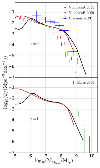
Figure 13: The Dust Mass Function (DMF) for redshifts $z=0$ and $1$. The black line shows the prediction of our model using the underlying dark matter Millennium simulation, and the red line for Millennium-II. Observations are taken from Vlahakis et al. (2005) and Clemens et al. (2013) at $z=0$, and from Eales et al. (2009) for $z=1$.

Figure 13 shows the dust mass function at $z=0$. The red line shows the results of the Millennium-II simulation, and the black line the Millennium simulation. We compare with observations from Vlahakis et al. (2005), Clemens et al. (2013) and Eales et al. (2009). Vlahakis et al. (2005) derived the local sub-mm luminosity and dust mass functions using the SCUBA (the Submillimetre Common-User Bolometer Array) Local Universe Galaxy Survey (SLUGS) and the IRAS Point Source Catalog Redshift Survey (PSCz). They fit two component grey bodies to their SEDs with emissivity index $\beta=2$ and dust temperature in the range 17-24 K. The ‘A’ sample determines dust masses using a dust temperature obtained from isothermal SED fitting, and the ‘B’ dust mass function has been calculated using a dust temperature of 20 K. Clemens et al. (2013) combined Herschel data with Wide-field Infrared Survey Explorer (WISE), Spitzer and Infrared Astronomical Satellite (IRAS) observations to investigate the properties of a flux-limited sample of local star-forming galaxies. They fit their SEDs with modified blackbody spectra using $\beta\simeq 2$ and dust temperatures in the range 10-25 K. Eales et al. (2009) uses data obtained from the Balloon-borne Large Aperture Submillimeter Telescope (BLAST), using the greybody relation assuming a dust temperature of 20K.

We find that the model provides a good fit to the Vlahakis et al. (2005) observations at low and intermediate dust masses, but under-predicts the number density when compared with Clemens et al. (2013) at the same mass range. The knee of the mass function is at a lower mass in Vlahakis et al. (2005) compared to our model output, while in Clemens et al. (2013) it roughly coincides with our model. At the high mass end, our predicted number densities are higher than both the observational data sets. This result is consistent with that of the previous section, that we over-predict the dust content of many massive galaxies at $z=0$ in our model. On comparing our model predictions to the Eales et al. (2009) data for $z=1$, we instead appear to slightly under-predict the dust mass function at high masses. It is worthwhile to note that this is a general feature seen in other models of galaxy formation tracking dust growth (e.g.  McKinnon et al. 2016, PSG17).

6 Conclusions

We have run a modified version of the L-Galaxies semi-analytic model which includes a prescription of dust modelling on the full Millennium and Millennium-II trees. By combining both the Millennium simulations we are able to make use of both the higher volume in order to find rarer objects, but also the higher mass resolution of Millennium-II to probe lower mass galaxies. Our conclusions are as follows:

1. Our grain growth model follows that of previous work, as described in Popping et al. (2017), but following separately the dust content in molecular clouds and the inter-cloud medium. We find that, in regimes where $\tau_{\rm{exch}}\gg\tau_{\rm{acc}}$ as well as for low values of $\mu$, this can have a significant impact upon the dust growth rate (Figure 1).

2. The dust-to-metal (DTM) ratio (Figure 3) shows an evolution from low to high ratios, the former corresponding to dust injection from type II supernovae, and the other to maximal, saturated dust production occurring via dust growth on grains. The latter dominates at redshifts below $z\approx 4$. A significantly populated transition region is seen at $z=6$.

3. By colouring with age (Figure 5) we show that this is the primary driver of the movement from low to high DTM ratio.

4. When plotted as a function of gas-phase metallicity, we find a reasonable fit to the observations at all redshifts (Figure 6).

5. We present a fitting relation for the DTM ratio, dependent on the metallicity and mass-weighted age of the galaxy stellar population. That provides a good fit to the model at both low and high redshift, but with some scatter at intermediate redshifts due to the varied growth histories of galaxies (Equation 15 and Figure 7).

6. Grain growth is the dominant dust production mechanism at all redshifts below $z=8$ (Figure 8). Dust destruction rate closely follows the grain growth production rate, suggesting prompt recycling of any dust content. We note, however, that Figure 3 shows that by $z=6$ only half of galaxies lie on the upper locus of DTM-ratio. Thus the detailed history of galaxy formation is important for determining the dust content of any individual galaxy.

7. The dust growth rates show little dependence on galaxy mass (Figure 9).

8. We find a good fit to the shape and normalisation of the dust-to-gas ratio at $z=0$ when plotted as a function of both stellar mass (Figure 10) and oxygen abundance (Figure 11).

9. We find a reasonable fit to the shape and normalisation of the observations in the stellar-dust mass plot (Figure 12) over a wide range of redshifts, $z=0-4$. We have an excess of very dusty, massive galaxies at $z=0$, perhaps due to a lack of destruction mechanisms. we fail to predict the dustiest galaxies at $z>5$, which hints that our dust growth rate may be too slow, or the destruction rate too high; however, we note that the interpretation of the observations are very uncertain at these redshifts.

10. There is a good agreement between the predicted $z=0$ dust mass function at the intermediate and low dust masses with observations; however we over predict the number density of galaxies at the highest dust masses (Figure 13). This again suggests that we may have too much dust in the most massive galaxies.

The model that we have presented here is deficient in at least 2 respects. Firstly, it assumes that dust is instantly destroyed in the hot (coronal) phase of the interstellar medium. Secondly, we ignore the effect of dust on the physics of galaxy formation: the formation of molecules on grains, and the coupling to radiative feedback, for example. This will be investigated in future work.

It seems evident from our work that, at sufficiently high redshift, there will be a transition from high (saturated dust growth) to much lower (primarily type II supernovae) dust-to-metal ratios. The precise redshift at which this happens depends upon uncertain grain growth and destruction time-scales. Nonetheless, it is important to appreciate that there will be a wide variety of DTM ratios in galaxies at high redshift. The situation will become much clearer over the next few years with deep extragalactic surveys such as those proposed by EUCLID, WFIRST and JWST and follow-up with ground-based observations from facilities such as ALMA.

Supporting Information

The required code to run the L-Galaxies version with the dust model can be found at https://github.com/aswinpvijayan/L-Galaxies_Dust.
Also the code to make the plots seen here can be found at https://github.com/aswinpvijayan/LGalaxies_paper_plots.

Appendix A Accretion Timescale

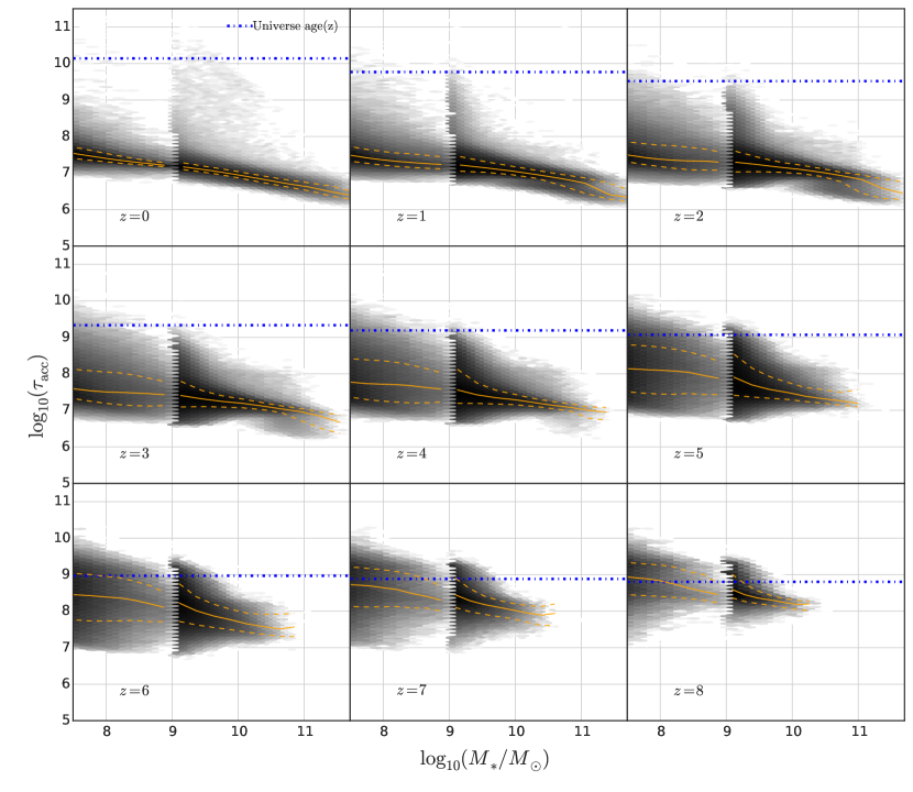
Figure 14: The accretion timescale-stellar mass relation for redshifts $z=0-8$. The orange lines show the median result from galaxies in our model and the 1-sigma scatter. The age of the Universe at that particular redshift is shown as the dot-dashed blue line.

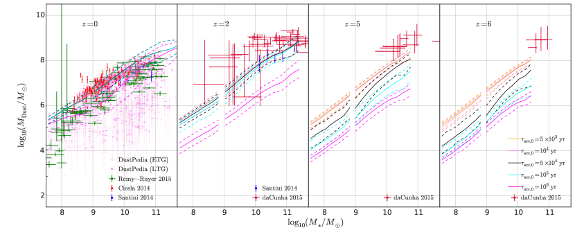
Figure 15: The median dust-stellar relation in our model for different values of $\tau_{\rm{acc,0}}$ at $z=0$, 2, 5 and 6. The solid line shows the median relation while the dashed lines denotes the 84 and 16 percentiles. The observational constraints from the DustPedia archive (see Davies et al., 2017, separated into ETGs and LTGs), Ciesla et al. (2014), Rémy-Ruyer et al. (2015), Santini et al. (2014) and da Cunha et al. (2015) respectively have been plotted for comparison.

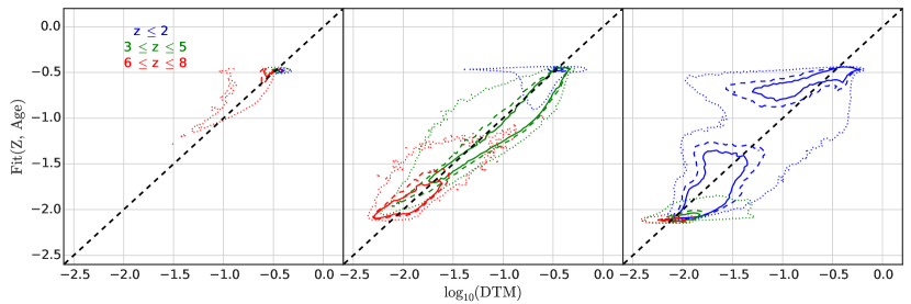
Figure 16: The DTM fitting function in Equation 15 is plotted against the DTM ratio from the model, similar to Figure 7. From left to right DTM values generated by running our model for $\tau_{\rm{acc,0}}$ values of 10⁴, 10⁵ and 10⁶ yr respectively are plotted against the fit function.

Here we will discuss how the accretion timescale varies with redshift as well the impact of choosing a different $\tau_{\rm{acc,0}}$ on our dust model.

Figure 14 shows the distribution of $\tau_{\rm{acc}}$ plotted against stellar mass for $z=0-8$. The age of the Universe at each redshift is also plotted for comparison. The median value of $\tau_{\rm{acc}}$ moves towards lower values as we move to lower redshifts due to the increase in the DTG ratio (see equation 11). Note that there are a lot of galaxies at high redshift ($z\geq 6$) that have $\tau_{\rm{acc}}$ values similar to the age of the Universe at that particular redshift – this is also the reason for very low values of DTG or DTM ratio, with comparable or higher values of the stellar production rate compared to grain growth. As we move towards lower redshift, most $\tau_{\rm{acc}}$ values start to dip beneath the age of the Universe and at $z\leq 2$ the median values are 3 to 4 orders of magnitude less than the age of the Universe. Thus the choice of $\tau_{\rm{acc,0}}$ has a negligible effect at low redshifts but can be be quite significant in determining the galaxy dust mass at high redshifts.

To see the effect of modifying the value of $\tau_{\rm{acc,0}}$ on the galaxy dust mass we consider values ranging from $5\times 10^{3}-10^{6}$ yr. The median dust-stellar mass relation for $z=0$, 2, 5 and 6 with these accretion timescales are shown in Figure 15. The dust-stellar mass relation at $z=0$ is not drastically affected by changes in $\tau_{\rm{acc,0}}$, except for $\tau_{\rm{acc,0}}=10^{6}$ yr where the median is about 0.5 dex lower than the other median values at intermediate stellar masses – this is because the dust growth timescale becomes comparable to the destruction timescale. Similarly, at $z=2$ the DTM ratio for $\tau_{\rm{acc,0}}=10^{6}$ yr has decreased by more than an order of magnitude. At $z=5$ and 6 the changes are more visible with a spread in DTM ratios becoming apparent as $\tau_{\rm{acc,0}}$ is varied. The main point to take away from this is that grain growth requires time to act, and that timescale depends on the value of $\tau_{\rm{acc,0}}$.

We also compare how our fitting function, Equation 15 performs for different values of $\tau_{\rm{acc,0}}$ in Figure 16. For this we ran our model with $\tau_{\rm{acc,0}}$ values of 10⁴, 10⁵ and 10⁶ yr, and obtain the expected DTM ratio using the corresponding $\tau_{\rm{acc,0}}$ values in Equation 15. We see that the fit does a good job for $\tau_{\rm{acc,0}}=10^{4}$ yr where we expect DTM ratios to be near saturation, while for the higher $\tau_{\rm{acc,0}}$ values we see considerable scatter in the fit. This scatter for $\tau_{\rm{acc,0}}=10^{6}$ yr directly follows from our previous discussion of the grain growth timescales. This has led to a bimodal distribution at $z\leq 2$, with the grain growth dominated population at the top and the stellar injection dominated ones at the bottom. The sharp cut-off in the bottom population is an artifact of our fitting function, as it can not have values less than $\mathcal{D}_{0}$.

References

- Aoyama et al. (2017) Aoyama S., Hou K. C., Shimizu I., Hirashita H., Todoroki K., Choi J. H., Nagamine K., 2017, MNRAS, 466, 105
- Arrigoni et al. (2010) Arrigoni M., Trager S. C., Somerville R. S., Gibson B. K., 2010, MNRAS, 402, 173
- Asplund et al. (2009) Asplund M., Grevesse N., Sauval A. J., Scott P., 2009, ARA&A, 47, 481
- Bekki (2013) Bekki K., 2013, MNRAS, 432, 2298
- Bernstein et al. (2002) Bernstein R. A., Freedman W. L., Madore B. F., 2002, ApJ, 571, 56
- Blitz & Rosolowsky (2006) Blitz L., Rosolowsky E., 2006, ApJ, 650, 933
- Boselli et al. (2010) Boselli A., et al., 2010, PASP, 122, 261
- Boylan-Kolchin et al. (2009) Boylan-Kolchin M., Springel V., White S. D. M., Jenkins A., Lemson G., 2009, MNRAS, 398, 1150
- Casey et al. (2014) Casey C. M., et al., 2014, ApJ, 796, 95
- Chabrier (2003) Chabrier G., 2003, PASP, 115, 763
- Ciesla et al. (2014) Ciesla L., et al., 2014, A&A, 565, A128
- Clemens et al. (2013) Clemens M. S., et al., 2013, MNRAS, 433, 695
- Dale et al. (2012) Dale D. A., et al., 2012, ApJ, 745, 95
- Davé et al. (2019) Davé R., Anglés-Alcázar D., Narayanan D., Li Q., Rafieferantsoa M. H., Appleby S., 2019, MNRAS, 486, 2827
- Davies et al. (2017) Davies J. I., et al., 2017, PASP, 129, 044102
- De Boer et al. (1987) De Boer K. S., Jura M. A., Shull J. M., 1987, Diffuse and Dark Clouds in the Interstellar Medium. Springer Netherlands, Dordrecht, pp 485–515
- De Cia et al. (2016) De Cia A., Ledoux C., Mattsson L., Petitjean P., Srianand R., Gavignaud I., Jenkins E. B., 2016, A&A, 596, A97
- De Lucia et al. (2014) De Lucia G., Tornatore L., Frenk C. S., Helmi A., Navarro J. F., White S. D. M., 2014, MNRAS, 445, 970
- De Vis et al. (2019) De Vis P., et al., 2019, A&A, 623, A5
- Draine & Li (2007) Draine B., Li A., 2007, ApJ, 657, 810
- Draine et al. (2014) Draine B. T., et al., 2014, ApJ, 780, 172
- Dunlop et al. (2017) Dunlop J. S., et al., 2017, MNRAS, 466, 861
- Dwek (1998) Dwek E., 1998, ApJ, 501, 643
- Dwek et al. (2014) Dwek E., Staguhn J., Arendt R. G., Kovacks A., Su T., Benford D. J., 2014, ApJl, 788, L30
- Eales et al. (2009) Eales S., et al., 2009, ApJ, 707, 1779
- Ferrarotti & Gail (2006) Ferrarotti A. S., Gail H.-P., 2006, A&A, 447, 553
- Franco et al. (2018) Franco M., et al., 2018, A&A, 620, A152
- Fu et al. (2013) Fu J., et al., 2013, MNRAS, 434, 1531
- Galliano, F. et al. (2011) Galliano, F. et al., 2011, A&A, 536, A88
- Gjergo et al. (2018) Gjergo E., Granato G. L., Murante G., Ragone-Figueroa C., Tornatore L., Borgani S., 2018, MNRAS, 479, 2588
- Greve et al. (2005) Greve T. R., et al., 2005, MNRAS, 359, 1165
- Groves et al. (2004) Groves B. A., Dopita M. A., Sutherland R. S., 2004, ApJS, 153, 75
- Gutiérrez & López-Corredoira (2014) Gutiérrez C. M., López-Corredoira M., 2014, A&A, 571, A66
- Gutkin et al. (2016) Gutkin J., Charlot S., Bruzual G., 2016, MNRAS, 462, 1757
- Henriques et al. (2015) Henriques B. M. B., White S. D. M., Thomas P. A., Angulo R., Guo Q., Lemson G., Springel V., Overzier R., 2015, MNRAS, 451, 2663
- Hirashita et al. (2018) Hirashita H., Aoyama S., Hou K.-C., Shimizu I., Nagamine K., 2018, MNRAS, 478, 4905
- Hodge et al. (2013) Hodge J. A., et al., 2013, ApJ, 768, 91
- Hou et al. (2019) Hou K.-C., Aoyama S., Hirashita H., Nagamine K., Shimizu I., 2019, MNRAS, 485, 1727
- Hu et al. (2019) Hu C.-Y., Zhukovska S., Somerville R. S., Naab T., 2019, arXiv e-prints, p. arXiv:1902.01368
- Inoue (2003) Inoue A. K., 2003, PASJ, 55, 901
- Irvine et al. (1987) Irvine W. M., Goldsmith P. F., Hjalmarson Å., 1987, in Hollenbach D. J., Thronson H. A., eds, Interstellar Processes. Springer Netherlands, Dordrecht, pp 560–609
- Jenkins (2009) Jenkins E. B., 2009, ApJ, 700, 1299
- Jones (2000) Jones A. P., 2000, Journal of Geophysical Research: Space Physics, 105, 10257
- Kennicutt et al. (2011) Kennicutt R. C., et al., 2011, PASP, 123, 1347
- Lakićević et al. (2015) Lakićević M., et al., 2015, ApJ, 799, 50
- Madden et al. (2013) Madden S. C., et al., 2013, PASP, 125, 600
- Mancini et al. (2015) Mancini M., Schneider R., Graziani L., Valiante R., Dayal P., Maio U., Ciardi B., Hunt L. K., 2015, MNRAS, 451, L70
- Mancini et al. (2016) Mancini M., Schneider R., Graziani L., Valiante R., Dayal P., Maio U., Ciardi B., 2016, MNRAS, 462, 3130
- Marigo (2001) Marigo P., 2001, A&A, 370, 194
- Martindale et al. (2017) Martindale H., Thomas P. A., Henriques B. M., Loveday J., 2017, MNRAS, 472, 1981
- Mattsson (2015) Mattsson L., 2015, preprint, (arXiv:1505.04758)
- McKee (1989) McKee C. F., 1989, ApJ, 345, 782
- McKee & Krumholz (2009) McKee C. F., Krumholz M. R., 2009, ApJ, 709, 308
- McKinnon et al. (2016) McKinnon R., Torrey P., Vogelsberger M., 2016, MNRAS, 457, 3775
- McKinnon et al. (2017) McKinnon R., Torrey P., Vogelsberger M., Hayward C. C., Marinacci F., 2017, MNRAS, 468, 1505
- McKinnon et al. (2018) McKinnon R., Vogelsberger M., Torrey P., Marinacci F., Kannan R., 2018, MNRAS, 478, 2851
- Michałowski (2015) Michałowski M. J., 2015, A&A, 577, A80
- Morgan & Edmunds (2003) Morgan H. L., Edmunds M. G., 2003, MNRAS, 343, 427
- Mortlock et al. (2011) Mortlock D. J., et al., 2011, Nature, 474, 616
- Nozawa et al. (2011) Nozawa T., Maeda K., Kozasa T., Tanaka M., Nomoto K., Umeda H., 2011, ApJ, 736, 45
- Peek et al. (2015) Peek J. E. G., Ménard B., Corrales L., 2015, ApJ, 813, 7
- Pillepich et al. (2018) Pillepich A., et al., 2018, MNRAS, 473, 4077
- Planck Collaboration et al. (2014) Planck Collaboration et al., 2014, A&A, 571, A1
- Popping et al. (2017) Popping G., Somerville R. S., Galametz M., 2017, MNRAS, 471, 3152
- Portinari et al. (1998) Portinari L., Chiosi C., Bressan A., 1998, A&A, 334, 505
- Rémy-Ruyer et al. (2014) Rémy-Ruyer A., et al., 2014, A&A, 563, A31
- Rémy-Ruyer et al. (2015) Rémy-Ruyer A., et al., 2015, A&A, 582, A121
- Santini et al. (2014) Santini P., et al., 2014, A&A, 562, A30
- Savage & Sembach (1996) Savage B. D., Sembach K. R., 1996, ApJ, 470, 893
- Schaerer et al. (2015) Schaerer D., Boone F., Zamojski M., Staguhn J., Dessauges-Zavadsky M., Finkelstein S., Combes F., 2015, A&A, 574, A19
- Scott et al. (2011) Scott K. S., et al., 2011, ApJ, 733, 29
- Scoville et al. (2016) Scoville N., et al., 2016, The Astrophysical Journal, 820, 83
- Somerville & Primack (1999) Somerville R. S., Primack J. R., 1999, MNRAS, 310, 1087
- Springel et al. (2005a) Springel V., et al., 2005a, Nature, 435, 629
- Springel et al. (2005b) Springel V., et al., 2005b, Nature, 435, 629
- Tacconi et al. (2006) Tacconi L. J., et al., 2006, ApJ, 640, 228
- Thielemann et al. (2003) Thielemann F.-K., et al., 2003, Nuclear Physics A, 718, 139
- Tinsley (1980) Tinsley B. M., 1980, A&A, 89, 246
- Tsai & Mathews (1995) Tsai J. C., Mathews W. G., 1995, ApJ, 448, 84
- Venemans et al. (2012) Venemans B. P., et al., 2012, ApJ, 751, L25
- Vlahakis et al. (2005) Vlahakis C., Dunne L., Eales S., 2005, MNRAS, 364, 1253
- Vogelsberger et al. (2013) Vogelsberger M., Genel S., Sijacki D., Torrey P., Springel V., Hernquist L., 2013, MNRAS, 436, 3031
- Watson et al. (2015) Watson D., Christensen L., Knudsen K. K., Richard J., Gallazzi A., Michałowski M. J., 2015, NATURE, 519, 327
- Wiersma et al. (2009) Wiersma R. P. C., Schaye J., Theuns T., Dalla Vecchia C., Tornatore L., 2009, MNRAS, 399, 574
- Wilkins et al. (2017) Wilkins S. M., Feng Y., Di Matteo T., Croft R., Lovell C. C., Thomas P., 2017, MNRAS, 473, 5363
- Wiseman et al. (2017) Wiseman P., Schady P., Bolmer J., Krühler T., Yates R. M., Greiner J., Fynbo J. P. U., 2017, A&A, 599, A24
- Yates et al. (2013) Yates R. M., Henriques B., Thomas P. A., Kauffmann G., Johansson J., White S. D. M., 2013, MNRAS, 435, 3500
- Yates et al. (2017) Yates R. M., Thomas P. A., Henriques B. M. B., 2017, MNRAS, 464, 3169
- Zhukovska (2014) Zhukovska S., 2014, A&A, 562, A76
- Zhukovska & Henning (2013) Zhukovska S., Henning T., 2013, A&A, 555, A99
- Zhukovska et al. (2008) Zhukovska S., Gail H.-P., Trieloff M., 2008, A&A, 479, 453
- Zubko et al. (2004) Zubko V., Dwek E., Arendt R. G., 2004, ApJS, 152, 211
- da Cunha et al. (2008) da Cunha E., Charlot S., Elbaz D., 2008, MNRAS, 388, 1595
- da Cunha et al. (2013) da Cunha E., et al., 2013, ApJ, 766, 13
- da Cunha et al. (2015) da Cunha E., et al., 2015, ApJ, 806, 110
- van Dishoeck & Blake (1998) van Dishoeck E. F., Blake G. A., 1998, ARA&A, 36, 317