HopSkipJumpAttack: A Query-Efficient Decision-Based Attack
Abstract
The goal of a decision-based adversarial attack on a trained model is to generate adversarial examples based solely on observing output labels returned by the targeted model. We develop HopSkipJumpAttack, a family of algorithms based on a novel estimate of the gradient direction using binary information at the decision boundary. The proposed family includes both untargeted and targeted attacks optimized for and similarity metrics respectively. Theoretical analysis is provided for the proposed algorithms and the gradient direction estimate. Experiments show HopSkipJumpAttack requires significantly fewer model queries than several state-of-the-art decision-based adversarial attacks. It also achieves competitive performance in attacking several widely-used defense mechanisms.
I Introduction
Although deep neural networks have achieved state-of-the-art performance on a variety of tasks, they have been shown to be vulnerable to adversarial examples—that is, maliciously perturbed examples that are almost identical to original samples in human perception, but cause models to make incorrect decisions [1]. The vulnerability of neural networks to adversarial examples implies a security risk in applications with real-world consequences, such as self-driving cars, robotics, financial services, and criminal justice; in addition, it highlights fundamental differences between human learning and existing machine-based systems. The study of adversarial examples is thus necessary to identify the limitation of current machine learning algorithms, provide a metric for robustness, investigate the potential risk, and suggest ways to improve the robustness of models.
Recent years have witnessed a flurry of research on the design of new algorithms for generating adversarial examples [1, 2, 3, 4, 5, 6, 7, 8, 9, 10, 11, 12, 13, 14, 15, 16]. Adversarial examples can be categorized according to at least three different criteria: the similarity metric, the attack goal, and the threat model. Commonly used similarity metrics are -distances between adversarial and original examples with . The goal of attack is either untargeted or targeted. The goal of an untargeted attack is to perturb the input so as to cause any type of misclassification, whereas the goal of a targeted attack is to alter the decision of the model to a pre-specific target class. Changing the loss function allows for switching between two types of attacks [3, 5, 6].
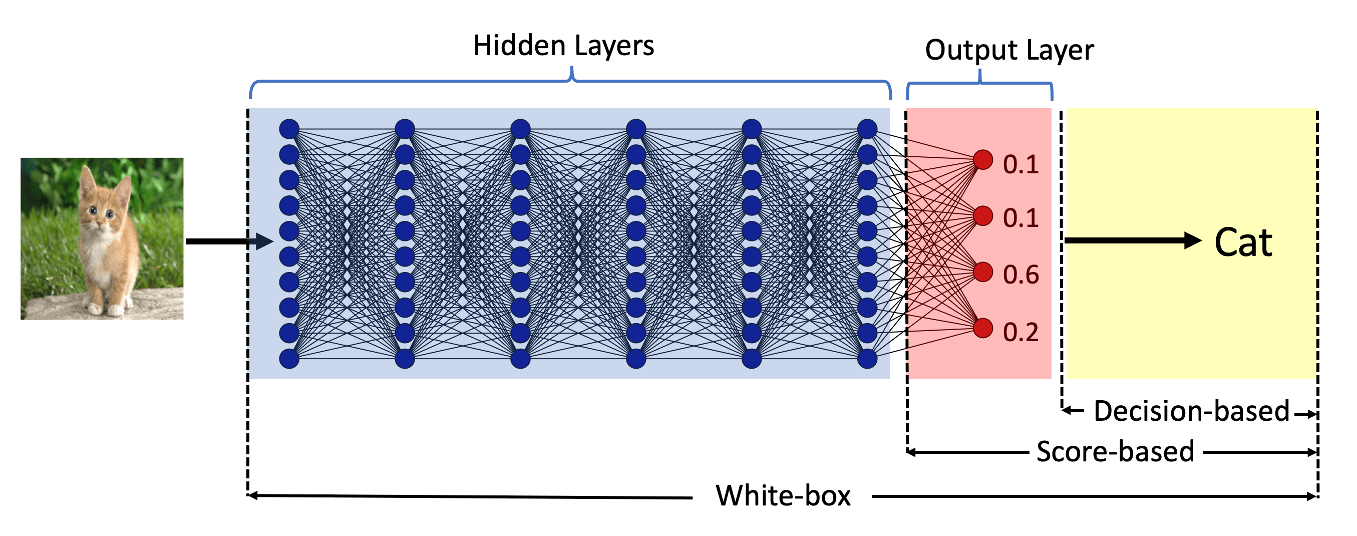
Perhaps the most important criterion in practice is the threat model, of which there are two primary types: white-box and black-box. In the white-box setting, an attacker has complete access to the model, including its structure and weights. Under this setting, the generation of adversarial examples is often formulated as an optimization problem, which is solved either via treating misclassification loss as a regularization [1, 6] or via tackling the dual as a constrained optimization problem [2, 3, 7]. In the black-box setting, an attacker can only access outputs of the target model. Based on whether one has access to the full probability or the label of a given input, black-box attacks are further divided into score-based and decision-based. See Figure 1 for an illustration of accessible components of the target model for each of the three threat models. Chen et al. [8] and Ilyas et al. [9, 10] introduced score-based methods using zeroth-order gradient estimation to craft adversarial examples.
The most practical threat model is that in which an attacker has access to decisions alone. A widely studied type of the decision-based attack is transfer-based attack. Liu et al. [11] showed that adversarial examples generated on an ensemble of deep neural networks from a white-box attack can be transferred to an unseen neural network. Papernot et al. [12, 13] proposed to train a substitute model by querying the target model. However, transfer-based attack often requires a carefully-designed substitute model, or even access to part of the training data. Moreover, they can be defended against via training on a data set augmented by adversarial examples from multiple static pre-trained models [17]. In recent work, Brendel et al. [14] proposed Boundary Attack, which generates adversarial examples via rejection sampling. While relying neither on training data nor on the assumption of transferability, this attack method achieves comparable performance with state-of-the-art white-box attacks such as C&W attack [6]. One limitation of Boundary Attack, however, is that it was formulated only for -distance. Moreover, it requires a relatively large number of model queries, rendering it impractical for real-world applications.
It is more realistic to evaluate the vulnerability of a machine learning system under the decision-based attack with a limited budget of model queries. Online image classification platforms often set a limit on the allowed number of queries within a certain time period. For example, the cloud vision API from Google currently allow 1,800 requests per minute. Query inefficiency thus leads to clock-time inefficiency and prevents an attacker from carrying out large-scale attacks. A system may also be set to recognize the behavior of feeding a large number of similar queries within a small amount of time as a fraud, which will automatically filter out query-inefficient decision-based attacks. Last but not least, a smaller query budget directly implies less cost in evaluation and research. Query-efficient algorithms help save the cost of evaluating the robustness of public platforms, which incur a cost for each query made by the attacker. It also helps facilitate research in adversarial vulnerability, as such a decision-based attack which does not require access to model details may be used as a simple and efficient first step in evaluating new defense mechanisms, as we will see in Section V-B and Appendix C.
In this paper, we study decision-based attacks under an optimization framework, and propose a novel family of algorithms for generating both targeted and untargeted adversarial examples that are optimized for minimum distance with respect to either the -distance or distance. The family of algorithms is iterative in nature, with each iteration involving three steps: estimation of the gradient direction, step-size search via geometric progression, and Boundary search via a binary search. Theoretical analysis has been carried out for the optimization framework and the gradient direction estimate, which not only provides insights for choosing hyperparamters, but also motivating essential steps in the proposed algorithms. We refer to the algorithm as HopSkipJumpAttack111A hop, skip, and a jump originally referred to an exercise or game involving these movements dating from the early 1700s, but by the mid-1800s it was also being used figuratively for the short distance so covered.. In summary, our contributions are the following:
-
•
We propose a novel unbiased estimate of gradient direction at the decision boundary based solely on access to model decisions, and propose ways to control the error from deviation from the boundary.
-
•
We design a family of algorithms, HopSkipJumpAttack, based on the proposed estimate and our analysis, which is hyperparameter-free, query-efficient and equipped with a convergence analysis.
-
•
We demonstrate the superior efficiency of our algorithm over several state-of-the-art decision-based attacks through extensive experiments.
-
•
Through the evaluation of several defense mechanisms such as defensive distillation, region-based classification, adversarial training and input binarization, we suggest our attack can be used as a simple and efficient first step for researchers to evaluate new defense mechanisms.
Roadmap. In Section II, we describe previous work on decision-based adversarial attacks and their relationship to our algorithm. We also discuss the connection of our algorithm to zeroth-order optimization. In Section III, we propose and analyze a novel iterative algorithm which requires access to the gradient information. Each step carries out a gradient update from the boundary, and then projects back to the boundary again. In Section IV, we introduce a novel asymptotically unbiased gradient-direction estimate at the boundary, and a binary-search procedure to approach the boundary. We also discuss how to control errors with deviation from the boundary. The analysis motivates a decision-based algorithm, HopSkipJumpAttack (Algorithm 2). Experimental results are provided in Section V. We conclude in Section VI with a discussion of future work.
II Related work
II-A Decision-based attacks
Most related to our work is the Boundary Attack method introduced by Brendel et al. [14]. Boundary Attack is an iterative algorithm based on rejective sampling, initialized at an image that lies in the target class. At each step, a perturbation is sampled from a proposal distribution, which reduces the distance of the perturbed image towards the original input. If the perturbed image still lies in the target class, the perturbation is kept. Otherwise, the perturbation is dropped. Boundary Attack achieves performance comparable to state-of-the-art white-box attacks on deep neural networks for image classification. The key obstacle to its practical application is, however, the demand for a large number of model queries. In practice, the required number of model queries for crafting an adversarial example directly determines the level of the threat imposed by a decision-based attack. One source of inefficiency in Boundary Attack is the rejection of perturbations which deviate from the target class. In our algorithm, the perturbations are used for estimation of a gradient direction.
Several other decision-based attacks have been proposed to improve efficiency. Brunner et al. [15] introduced Biased Boundary Attack, which biases the sampling procedure by combining low-frequency random noise with the gradient from a substitute model. Biased Boundary Attack is able to significantly reduce the number of model queries. However, it relies on the transferability between the substitute model and the target model, as with other transfer-based attacks. Our algorithm does not rely on the additional assumption of transferability. Instead, it achieves a significant improvement over Boundary Attack through the exploitation of discarded information into the gradient-direction estimation. Ilyas et al. [9] proposed Limited attack in the label-only setting, which directly performs projected gradient descent by estimating gradients based on novel proxy scores. Cheng et al. [16] introduced Opt attack, which transforms the original problem to a continuous version, and solves the new problem via randomized zeroth-order gradient update. Our algorithm approaches the original problem directly via a novel gradient-direction estimate, leading to improved query efficiency over both Limited Attack and Opt Attack. The majority of model queries in HopSkipJumpAttack come in mini-batches, which also leads to improved clock-time efficiency over Boundary Attack.
II-B Zeroth-order optimization
Zeroth-order optimization refers to the problem of optimizing a function based only on access to function values , as opposed to gradient values . Such problems have been extensively studied in the convex optimization and bandit literatures. Flaxman et al. [18] studied one-point randomized estimate of gradient for bandit convex optimization. Agarwal et al. [19] and Nesterov and Spokoiny [20] demonstrated that faster convergence can be achieved by using two function evaluations for estimating the gradient. Duchi et al. [21] established optimal rates of convex zeroth-order optimization via mirror descent with two-point gradient estimates. Zeroth-order algorithms have been applied to the generation of adversarial examples under the score-based threat model [8, 9, 10]. Subsequent work [22] proposed and analyzed an algorithm based on variance-reduced stochastic gradient estimates.
We formulate decision-based attack as an optimization problem. A core component of our proposed algorithm is a gradient-direction estimate, the design of which is motivated by zeroth-order optimization. However, the problem of decision-based attack is more challenging than zeroth-order optimization, essentially because we only have binary information from output labels of the target model, rather than function values.
III An optimization framework
In this section, we describe an optimization framework for finding adversarial instances for an -ary classification model of the following type. The first component is a discriminant function that accepts an input and produces an output . The output vector can be viewed as a probability distribution over the label set . Based on the function , the classifier assigns input to the class with maximum probability—that is,
We study adversaries of both the untargeted and targeted varieties. Given some input , the goal of an untargeted attack is to change the original classifier decision to any , whereas the goal of a targeted attack is to change the decision to some pre-specified . Formally, if we define the function via
| (1) |
then a perturbed image is a successful attack if and only if . The boundary between successful and unsuccessful perturbed images is
As an indicator of successful perturbation, we introduce the Boolean-valued function via
This function is accessible in the decision-based setting, as it can be computed by querying the classifier alone. The goal of an adversarial attack is to generate a perturbed sample such that , while keeping close to the original sample . This can be formulated as the optimization problem
| (2) |
where is a distance function that quantifies similarity. Standard choices of studied in past work [5, 2, 6] include the usual -norms, for .
III-A An iterative algorithm for distance
Consider the case of the optimization problem (2) with the -norm . We first specify an iterative algorithm that is given access to the gradient . Given an initial vector such that and a stepsize sequence , it performs the update
| (3) |
where is a positive step size. Here the line search parameter is chosen such that —that is, so that the next iterate lies on the boundary. The motivation for this choice is that our gradient-direction estimate in Section IV is only valid near the boundary.
We now analyze this algorithm with the assumption that we have access to the gradient of in the setting of binary classification. Assume that the function is twice differentiable with a locally Lipschitz gradient, meaning that there exists such that for all , we have
| (4) |
In addition, we assume the gradient is bounded away from zero on the boundary: there exists a positive such that for any .
We analyze the behavior of the updates (3) in terms of the angular measure
corresponding to the cosine of the angle between and the gradient . Note that the condition holds if and only if is a stationary point of the optimization (2). The following theorem guarantees that, with a suitable step size, the updates converge to such a stationary point:
Theorem 1.
Theorem 1 suggests a scheme for choosing the step size in the algorithm that we present in the next section. An experimental evaluation of the proposed scheme is carried out in Appendix B. The proof of the theorem is constructed by establishing the relationship between the objective value and , with a second-order Taylor approximation to the boundary. See Appendix A-A for details.
III-B Extension to -distance
We now describe how to extend these updates so as to minimize the -distance. Consider the -projection of a point onto the sphere of radius centered at :
| (6) |
In terms of this operator, our -based update (3) can be rewritten in the equivalent form
| (7) |
This perspective allows us to extend the algorithm to other -norms for . For instance, in the case , we can define the -projection operator . It performs a per-pixel clip within a neighborhood of , such that the th entry of is
where . We propose the -version of our algorithm by carrying out the following update iteratively:
| (8) |
where is chosen such that , and “sign” returns the element-wise sign of a vector. We use the sign of the gradient for faster convergence in practice, similar to previous work [2, 3, 7].
IV A decision-based algorithm based on a novel gradient estimate
We now extend our procedures to the decision-based setting, in which we have access only to the Boolean-valued function —that is, the method cannot observe the underlying discriminant function or its gradient. In this section, we introduce a gradient-direction estimate based on when (so that by definition). We proceed to discuss how to approach the boundary. Then we discuss how to control the error of our estimate with a deviation from the boundary. We will summarize the analysis with a decision-based algorithm.
IV-A At the boundary
Given an iterate we propose to approximate the direction of the gradient via the Monte Carlo estimate
| (9) |
where are i.i.d. draws from the uniform distribution over the -dimensional sphere, and is small positive parameter. (The dependence of this estimator on the fixed centering point is omitted for notational simplicity.)
The perturbation parameter is necessary, but introduces a form of bias in the estimate. Our first result controls this bias, and shows that is asymptotically unbiased as .
Theorem 2.
For a boundary point , suppose that has -Lipschitz gradients in a neighborhood of . Then the cosine of the angle between and is bounded as
| (10) |
In particular, we have
| (11) |
showing that the estimate is asymptotically unbiased as an estimate of direction.
We remark that Theorem 2 only establishes the asymptotic behavior of the proposed estiamte at the boundary. This also motivates the boundary search step in our algorithm to be discussed in Seciton IV-B. The proof of Theorem 2 starts from dividing the unit sphere into three components: the upper cap along the direction of gradient, the lower cap opposite to the direction of gradient, and the annulus in between. The error from the annulus can be bounded when is small. See Appendix A-B for the proof of this theorem. As will be seen in the sequel, the size of perturbation should be chosen proportionally to ; see Section IV-C for details.
IV-B Approaching the boundary
The proposed estimate (9) is only valid at the boundary. We now describe how we approach the boundary via a binary search. Let denote the updated sample before the operator is applied:
| (12) | ||||
where will be introduced later in equation (16), as a variance-reduced version of , and is the size of perturbation at the -th step.
We hope is at the opposite side of the boundary to so that the binary search can be carried out. Therefore, we initialize at at the target side with , and set , where is chosen via a binary search between and to approach the boundary, stopped at lying on the target side with . At the -th iteration, we start at lying at the target side . The step size is initialized as
| (13) |
as suggested by Theorem 1 in the case, and is decreased by half until , which we call geometric progression of . Having found an appropriate , we choose the projection radius via a binary search between and to approach the boundary, which stops at with . See Algorithm 1 for the complete binary search, where the binary search threshold is set to be some small constant.

IV-C Controlling errors of deviations from the boundary
Binary search never places exactly onto the boundary. We analyze the error of the gradient-direction estimate, and propose two approaches for reducing the error.
Appropriate choice of the size of random perturbation
First, the size of random perturbation for estimating the gradient direction is chosen as a function of image size and the binary search threshold . This is different from numerical differentiation, where the optimal choice of is at the scale of round-off errors (e.g., [23]). Below we characterize the error incurred by a large as a function of distance between and the boundary, and derive the appropriate choice of and . In fact, with a Taylor approximation of at , we have
At the boundary , the error of gradient approximation scales at , which is minimized by reducing to the scale of rooted round-off error. However, the outcome of a finite-step binary search lies close to, but not exactly on the boundary.
When is small enough such that second-order terms can be omitted, the first-order Taylor approximation implies that if and only if lies on the spherical cap , with
On the other hand, the probability mass of concentrates on the equator in a high-dimensional sphere, which is characterized by the following inequality [24]:
| (14) |
A Taylor expansion of at yields
By the Cauchy-Schwarz inequality and the definition of -projection, we have
This yields
where is the dual exponent. In order to avoid a loss of accuracy from concentration of measure, we let . To make the approximation error independent of dimension , we set at the scale of , so that is proportional to , as suggested by Theorem 2. This leads to a logarithmic dependence on dimension for the number of model queries. In practice, we set
| (15) |
| Distance | Data | Model | Objective | Model Queries | ||||||||
| 1K | 5K | 20K | ||||||||||
| BA | Opt | HSJA | BA | Opt | HSJA | BA | Opt | HSJA | ||||
| MNIST | CNN | Untargeted | 6.14 | 6.79 | 2.46 | 5.45 | 3.76 | 1.67 | 1.50 | 2.07 | 1.48 | |
| Targeted | 5.41 | 4.84 | 3.26 | 5.38 | 3.90 | 2.24 | 1.98 | 2.49 | 1.96 | |||
| CIFAR10 | ResNet | Untargeted | 2.78 | 2.07 | 0.56 | 2.34 | 0.77 | 0.21 | 0.27 | 0.29 | 0.13 | |
| Targeted | 7.83 | 8.21 | 2.53 | 5.91 | 4.76 | 0.41 | 0.59 | 1.06 | 0.21 | |||
| DenseNet | Untargeted | 2.57 | 1.78 | 0.48 | 2.12 | 0.67 | 0.18 | 0.21 | 0.28 | 0.12 | ||
| Targeted | 7.70 | 7.65 | 1.75 | 5.33 | 3.47 | 0.34 | 0.35 | 0.78 | 0.19 | |||
| CIFAR100 | ResNet | Untargeted | 1.34 | 1.20 | 0.20 | 1.12 | 0.41 | 0.08 | 0.10 | 0.14 | 0.06 | |
| Targeted | 9.30 | 12.43 | 6.12 | 7.40 | 8.34 | 0.92 | 1.61 | 4.06 | 0.29 | |||
| DenseNet | Untargeted | 1.47 | 1.22 | 0.25 | 1.23 | 0.34 | 0.11 | 0.12 | 0.13 | 0.08 | ||
| Targeted | 8.83 | 11.72 | 5.10 | 6.76 | 8.22 | 0.75 | 0.91 | 2.89 | 0.26 | |||
| ImageNet | ResNet | Untargeted | 36.86 | 33.60 | 9.75 | 31.95 | 13.91 | 2.30 | 2.71 | 5.26 | 0.84 | |
| Targeted | 87.49 | 84.38 | 71.99 | 82.91 | 71.83 | 38.79 | 40.92 | 53.78 | 10.95 | |||
| MNIST | CNN | Untargeted | 0.788 | 0.641 | 0.235 | 0.700 | 0.587 | 0.167 | 0.243 | 0.545 | 0.136 | |
| Targeted | 0.567 | 0.630 | 0.298 | 0.564 | 0.514 | 0.211 | 0.347 | 0.325 | 0.175 | |||
| CIFAR10 | ResNet | Untargeted | 0.127 | 0.128 | 0.023 | 0.105 | 0.096 | 0.008 | 0.019 | 0.073 | 0.005 | |
| Targeted | 0.379 | 0.613 | 0.134 | 0.289 | 0.353 | 0.028 | 0.038 | 0.339 | 0.010 | |||
| DenseNet | Untargeted | 0.114 | 0.119 | 0.017 | 0.095 | 0.078 | 0.007 | 0.017 | 0.063 | 0.004 | ||
| Targeted | 0.365 | 0.629 | 0.130 | 0.249 | 0.359 | 0.022 | 0.025 | 0.338 | 0.008 | |||
| CIFAR100 | ResNet | Untargeted | 0.061 | 0.077 | 0.009 | 0.051 | 0.055 | 0.004 | 0.008 | 0.040 | 0.002 | |
| Targeted | 0.409 | 0.773 | 0.242 | 0.371 | 0.472 | 0.124 | 0.079 | 0.415 | 0.019 | |||
| DenseNet | Untargeted | 0.065 | 0.076 | 0.010 | 0.055 | 0.038 | 0.005 | 0.010 | 0.030 | 0.003 | ||
| Targeted | 0.388 | 0.750 | 0.248 | 0.314 | 0.521 | 0.096 | 0.051 | 0.474 | 0.017 | |||
| ImageNet | ResNet | Untargeted | 0.262 | 0.287 | 0.057 | 0.234 | 0.271 | 0.017 | 0.030 | 0.248 | 0.007 | |
| Targeted | 0.615 | 0.872 | 0.329 | 0.596 | 0.615 | 0.219 | 0.326 | 0.486 | 0.091 | |||
A baseline for variance reduction in gradient-direction estimation
Another source of error comes from the variance of the estimate, where we characterize variance of a random vector by the trace of its covariance operator: . When deviates from the boundary and is not exactly zero, there is an uneven distribution of perturbed samples at the two sides of the boundary:
as we can see from Equation (14). To attempt to control the variance, we introduce a baseline into the estimate:
which yields the following estimate:
| (16) |
It can be easily observed that this estimate is equal to the previous estimate in expectation, and thus still asymptotically unbiased at the boundary: When , we have
Moreover, the introduction of the baseline reduces the variance when deviates from zero. In particular, the following theorem shows that whenever , the introduction of a baseline reduces the variance.
Theorem 3.
Defining as the variance of one-point estimate, we have
where
IV-D HopSkipJumpAttack
We now combine the above analysis into an iterative algorithm, HopSkipJumpAttack. It is initialized with a sample in the target class for untargeted attack, and with a sample blended with uniform noise that is misclassified for targeted attack. Each iteration of the algorithm has three components. First, the iterate from the last iteration is pushed towards the boundary via a binary search (Algorithm 1). Second, the gradient direction is estimated via Equation (16). Third, the updating step size along the gradient direction is initialized as Equation (13) based on Theorem 1, and is decreased via geometric progression until perturbation becomes successful. The next iteration starts with projecting the perturbed sample back to the boundary again. The complete procedure is summarized in Algorithm 2. Figure 2 provides an intuitive visualization of the three steps in . For all experiments, we initialize the batch size at and increase it with linearly, so that the variance of the estimate reduces with . When the input domain is bounded in practice, a clip is performed at each step by default.

V Experiments
In this section, we carry out experimental analysis of HopSkipJumpAttack. We compare the efficiency of HopSkipJumpAttack with several previously proposed decision-based attacks on image classification tasks. In addition, we evaluate the robustness of three defense mechanisms under our attack method. All experiments were carried out on a Tesla K80 GPU, with code available online.222See https://github.com/Jianbo-Lab/HSJA/. Our algorithm is also available on CleverHans [25] and Foolbox [26], which are two popular Python packages to craft adversarial examples for machine learning models.

V-A Efficiency evaluation
Baselines
We compare HopSkipJumpAttack with three state-of-the-art decision-based attacks: Boundary Attack [14], Limited Attack [9] and Opt Attack [16]. We use the implementation of the three algorithms with the suggested hyper-parameters from the publicly available source code online. Limited Attack is only included under the targeted setting, as in Ilyas et al. [9].

Data and models
For a comprehensive evaluation of HopSkipJumpAttack, we use a wide range of data and models, with varied image dimensions, data set sizes, complexity levels of task and model structures.
The experiments are carried out over four image data sets: MNIST, CIFAR-10 [27], CIFAR-100 [27], and ImageNet [28] with the standard train/test split [29]. The four data sets have varied image dimensions and class numbers. MNIST contains 70K gray-scale images of handwritten digits in the range 0-9. CIFAR-10 and CIFAR-100 are both composed of images. CIFAR-10 has 10 classes, with 6K images per class, while CIFAR-100 has 100 classes, with 600 images per class. ImageNet has classes. Images in ImageNet are rescaled to . For MNIST, CIFAR-10 and CIFAR-100, correctly classified test images are used, which are randomly drawn from the test data set, and evenly distributed across classes. For ImageNet, we use correctly classified test images, evenly distributed among randomly selected classes. The selection scheme follows Metzen et al. [30] for reproducibility.
We also use models of varied structure, from simple to complex. For MNIST, we use a simple convolutional network composed of two convolutional layers followed by a hidden dense layer with units. Two convolutional layers have filters respectively, each of which is followed by a max-pooling layer. For both CIFAR-10 and CIFAR-100, we train a -layer ResNet [31] and -layer DenseNet [32] respectively, with the canonical network structure [29]. For ImageNet, we use a pre-trained -layer ResNet [31]. All models achieve close to state-of-the-art accuracy on the respective data set. All pixels are scaled to be in the range . For all experiments, we clip the perturbed image into the input domain for all algorithms by default.
Initialization
For untargeted attack, we initialize all attacks by blending an original image with uniform random noise, and increasing the weight of uniform noise gradually until it is misclassified, a procedure which is available on Foolbox [26], as the default initialization of Boundary Attack. For targeted attack, the target class is sampled uniformly among the incorrect labels. An image belonging to the target class is randomly sampled from the test set as the initialization. The same target class and a common initialization image are used for all attacks.
Metrics
The first metric is the median distance between perturbed and original samples over a subset of test images, which was commonly used in previous work, such as Carlini and Wagner [6]. A version normalized by image dimension was employed by Brendel et al. [14] for evaluating Boundary Attack. The distance can be interpreted in the following way: Given a byte image of size , perturbation of size in distance on the rescaled input image amounts to perturbation on the original image of bits per pixel on average, in the range . The perturbation of size in distance amounts to a maximum perturbation of bits across all pixels on the raw image.
As an alternative metric, we also plot the success rate at various distance thresholds for both algorithms given a limited budget of model queries. An adversarial example is defined a success if the size of perturbation does not exceed a given distance threshold. The success rate can be directly related to the accuracy of a model on perturbed data under a given distance threshold:
| (17) |
Throughout the experiments, we limit the maximum budget of queries per image to 25,000, the setting of practical interest, due to limited computational resources.
Results
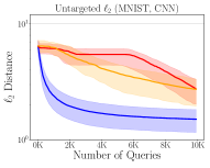
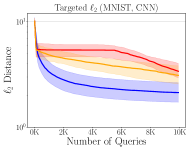
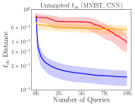
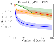
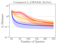
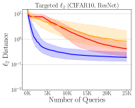
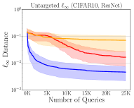
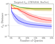
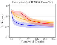
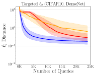
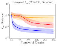
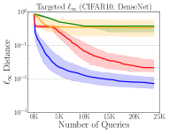
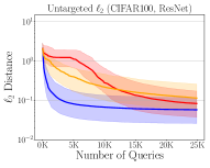
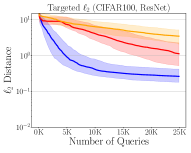
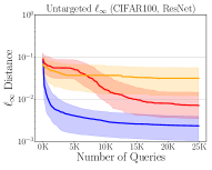
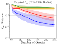
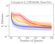
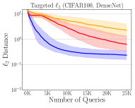
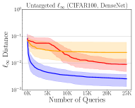
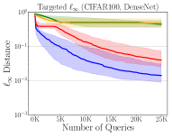
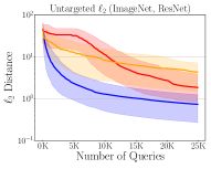
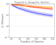
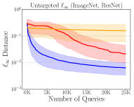
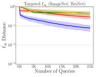
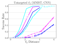
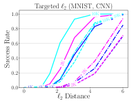
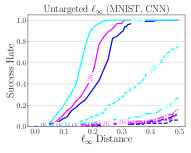
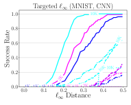
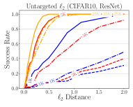
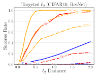
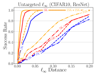
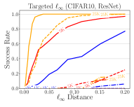
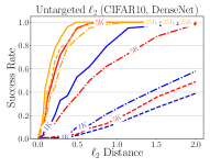
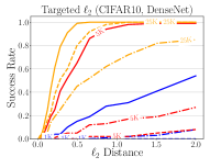
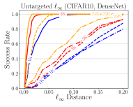
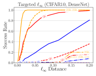
Figure 3 and 4 show the median distance (on a log scale) against the queries, with the first and third quartiles used as lower and upper error bars. For Boundary, Opt and HopSkipJumpAttack, Table I summarizes the median distance when the number of queries is fixed at 1,000, 5,000, and 20,000 across all distance types, data, models and objectives. Figure 5 and 6 show the success rate against the distance threshold. Figure 3 and 5 contain results on MNIST with CNN, and CIFAR-10 with ResNet, Denset, subsequently from the top row to the bottom row. Figure 4 and 6 contain results on CIFAR-100 with ResNet and DenseNet, and ImageNet with ResNet, subsequently from the top row to the bottom row. The four columns are for untargeted , targeted , untargeted and targeted attacks respectively.
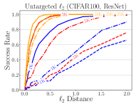
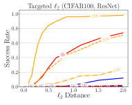
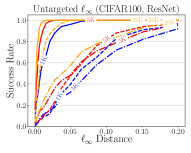
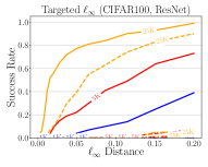
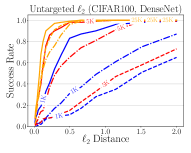
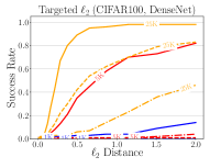
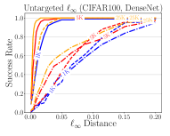
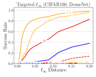
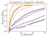
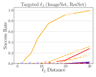
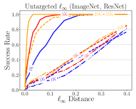
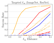

With a limited number of queries, HopSkipJumpAttack is able to craft adversarial examples of a significantly smaller distance with the corresponding original examples across all data sets, followed by Boundary Attack and Opt Attack. As a concrete example, Table I shows that untargeted -optimized HopSkipJumpAttack achieves a median distance of on CIFAR-10 with a ResNet model at queries, which amounts to below per pixel on average. At the same budget of queries, Boundary Attack and Opt Attack only achieve median -distances of and respectively. The difference in efficiency becomes more significant for attacks. As shown in Figure 5, under an untargeted -optimized HopSkipJumpAttack with 1,000 queries, all pixels are within an -neighborhood of the original image for around 70% of adversarial examples, a success rate achieved by Boundary Attack only after 20,000 queries.
By comparing the odd and even columns of Figure 3-6, we can find that targeted HopSkipJumpAttack takes more queries than the untargeted one to achieve a comparable distance. This phenomenon becomes more explicit on CIFAR-100 and ImageNet, which have more classes. With the same number of queries, there is an order-of-magnitude difference in median distance between untargeted and targeted attacks (Figure 3 and 4). For -optimized HopSkipJumpAttack, while the untargeted version is able to craft adversarial images by perturbing bits per pixel on average within 1,000 queries for of images in CIFAR-10 and CIFAR-100, the targeted counterpart takes 2,000-5,000 queries. The other attacks fail to achieve a comparable performance even with 25,000 queries. On ImageNet, untargeted -optimized HopSkipJumpAttack is able to fool the model with a perturbation of size bits per pixel on average for close to of images with queries; untargeted -optimized HopSkipJumpAttack controls the maximum perturbation across all pixels within bits for images within queries. The targeted Boundary Attack is not able to control the perturbation size to such a small scale until after around queries. On the one hand, the larger query budget requirement results from a strictly more powerful formulation of targeted attack than untargeted attack. On the other hand, this is also because we initialize targeted HopSkipJumpAttack from an arbitrary image in the target class. The algorithm may be trapped in a bad local minimum with such an initialization. Future work can address systematic approaches to better initialization.
As a comparison between data sets and models, we see that adversarial images often have a larger distance to their corresponding original images on MNIST than on CIFAR-10 and CIFAR-100, which has also been observed in previous work (e.g., [6]). This might be because it is more difficult to fool a model on simpler tasks. On the other hand, HopSkipJumpAttack also converges in a fewer number of queries on MNIST, as is shown in Figure 3. It does not converge even after queries on ImageNet. We conjecture the query budget is related to the input dimension, and the smoothness of decision boundary. We also observe the difference in model structure does not have a large influence on decision-based algorithms, if the training algorithm and the data set keep the same. For ResNet and DenseNet trained on a common data set, a decision-based algorithm achieves comparable performance in crafting adversarial examples, although DenseNet has a more complex structure than ResNet.
As a comparison with state-of-the-art white-box targeted attacks, C&W attack [6] achieves an average -distance of on CIFAR-10, and BIM [3] achieves an average -distance of on CIFAR-10. Targeted HopSkipJumpAttack achieves a comparable distance with 5K-10K model queries on CIFAR-10, without access to model details. On ImageNet, targeted C&W attack and BIM achieve an -distance of and an -distance of respectively. Untargeted HopSkipJumpAttack achieves a comparable performance with queries. The targeted version is not able to perform comparably as targeted white-box attacks when the budget of queries is limited within .
Visualized trajectories of HopSkipJumpAttack optimized for distances along varied queries on CIFAR10 and ImageNet can be found in Figure 7. On CIFAR-10, we observe untargeted adversarial examples can be crafted within around queries; targeted HopSkipJumpAttack is capable of crafting human indistinguishable targeted adversarial examples within around queries. On ImageNet, untargeted HopSkipJumpAttack is able to craft good adversarial examples with queries, while targeted HopSkipJumpAttack takes queries.


V-B Defense mechanisms under decision-based attacks
We investigate the robustness of various defense mechanisms under decision-based attacks.
Defense mechanisms
Three defense mechanisms are evaluated: defensive distillation, region-based classification, and adversarial training. Defensive distillation [33], a form of gradient masking [13], trains a second model to predict the output probabilities of an existing model of the same structure. We use the implementaion provided by Carlini and Wagner [6] for defensive distillation. The second defense, region-based classification, belongs to a wide family of mechanisms which add test-time randomness to the inputs or the model, causing the gradients to be randomized [34]. Multiple variants have been proposed to randomize the gradients [35, 36, 37, 38, 39]. We adopt the implementation in Cao and Gong [35] with suggested noise levels. Given a trained base model, region-based classification samples points from the hypercube centered at the input image, predicts the label for each sampled point with the base model, and then takes a majority vote to output the label. Adversarial training [2, 3, 7, 17] is known to be one of the most effective defense mechanisms against adversarial perturbation [40, 34]. We evaluate a publicly available model trained through a robust optimization method proposed by Madry et al. [7]. We further evaluate our attack method by constructing a non-differentiable model via input binarization followed by a random forest in Appendix C. The evaluation is carried out on MNIST, where defense mechanisms such as adversarial training work most effectively.
Baselines
We compare our algorithm with state-of-the-art attack algorithms that require access to gradients, including C&W Attack [6], DeepFool [4] for minimizing -distance, and FGSM [2], and BIM [41, 7] for minimizing -distance. For region-based classification, the gradient of the base classifier is taken with respect to the original input.
We further include methods designed specifically for the defense mechanisms under threat. For defensive distillation, we include the -optimized C&W Attack [6]. For region-based classification, we include backward pass differentiable approximation (BPDA) [34], which calculates the gradient of the model at a randomized input to replace the gradient at the original input in C&W Attack and BIM. All of these methods assume access to model details or even defense mechanisms, which is a stronger threat model than the one required for decision-based attacks. We also include Boundary Attack as a decision-based baseline.
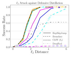
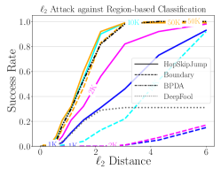
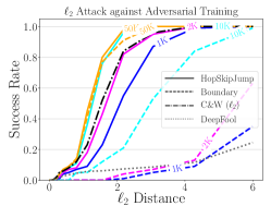
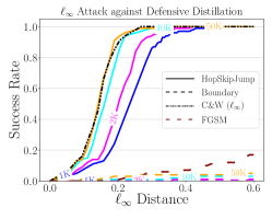
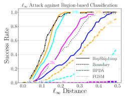
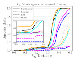
For HopSkipJumpAttack and Boundary Attack, we include the success rate at three different scales of query budget: 2K, 10K and 50K, so as to evaluate our method both with limited queries and a sufficient number of queries. We find the convergence of HopSkipJumpAttack becomes unstable on region-based classification, resulting from the difficulty of locating the boundary in the binary search step when uncertainty is increased near the boundary. Thus, we increase the binary search threshold to 0.01 to resolve this issue.
Results
Figure 8 shows the success rate of various attacks at different distance thresholds for the three defense mechanisms. On all of the three defenses, HopSkipJumpAttack demonstrates similar or superior performance compared to state-of-the-art white-box attacks with sufficient model queries. Even with only 1K-2K model queries, it also achieves acceptable performance, although worse than the best white-box attacks. With sufficient queries, Boundary Attack achieves a comparable performance under the -distance metric. But it is not able to generate any adversarial examples when the number of queries is limited to . We think this is because the strength of our batch gradient direction estimate over the random walk step in Boundary Attack becomes more explicit when there is uncertainty or non-smoothness near the decision boundary. We also observe that Boundary Attack does not work in optimizing the -distance metric for adversarial examples, making it difficult to evaluate defenses designed for distance, such as adversarial training proposed by Madry et al. [7].
On a distilled model, when the -distance is thresholded at , a perturbation size proposed by Madry et al. [7] to measure adversarial robustness, HopSkipJumpAttack achieves success rates of and with 1K and 50K queries respectively. At an -distance of 3.0, the success rate is with 2K queries. HopSkipJumpAttack achieves a comparable performance with C&W attack under both distance metrics with 10K-50K queries. Also, gradient masking [13] by defensive distillation does not have a large influence on the query efficiency of HopSkipJumpAttack, indicating that the gradient direction estimate is robust under the setting where the model does not have useful gradients for certain white-box attacks.
On region-based classification, with 2K queries, HopSkipJumpAttack achieves success rates of and at the same - and -distance thresholds respectively. With 10K-50K queries, it is able to achieve a comparable performance to BPDA, a white-box attack tailored to such defense mechanisms. On the other hand, we observe that HopSkipJumpAttack converges slightly slower on region-based classification than itself on ordinary models, which is because stochasticity near the boundary may prevent binary search in HopSkipJumpAttack from locating the boundary accurately.
On an adversarially trained model, HopSkipJumpAttack achieves a success rate of with 50K queries when the -distance is thresholded at . As a comparison, BIM has a success rate of at the given distance threshold. The success rate of -HopSkipJumpAttack transfers to an accuracy of on adversarially perturbed data, close to the state-of-the-art performance achieved by white-box attacks.333See https://github.com/MadryLab/mnist_challenge. With 1K queries, HopSkipJumpAttack also achieves comparable performance to BIM and C&W attack.
VI Discussion
We have proposed a family of query-efficient algorithms based on a novel gradient-direction estimate, HopSkipJumpAttack, for decision-based generation of adversarial examples, which is capable of optimizing and -distances for both targeted and untargeted attacks. Convergence analysis has been carried out given access to the gradient. We have also provided analysis for the error of our Monte Carlo estimate of gradient direction, which comes from three sources: bias at the boundary for a nonzero perturbation size, bias of deviation from the boundary, and variance. Theoretical analysis has provided insights for selecting the step size and the perturbation size, which leads to a hyperparameter-free algorithm. We have also carried out extensive experiments, showing HopSkipJumpAttack compares favorably to Boundary Attack in query efficiency, and achieves competitive performance on several defense mechanisms.
Given the fact that HopSkipJumpAttack is able to craft a human-indistinguishable adversarial example within a realistic budget of queries, it becomes important for the community to consider the real-world impact of decision-based threat models. We have also demonstrated that HopSkipJumpAttack is able to achieve comparable or even superior performance to state-of-the-art white-box attacks on several defense mechanisms, under a much weaker threat model. In particular, masked gradients, stochastic gradients, and non-differentiability are not barriers to our algorithm. Because of its effectiveness, efficiency, and applicability to non-differentiable models, we suggest future research on adversarial defenses may evaluate the designed mechanism against HopSkipJumpAttack as a first step.
One limitation of all existing decision-based algorithms, including HopSkipJumpAttack, is that they require evaluation of the target model near the boundary. They may not work effectively by limiting the queries near the boundary, or by widening the decision boundary through insertion of an additional “unknown” class for inputs with low confidence. We have also observed that it still takes tens of thousands of model queries for HopSkipJumpAttack to craft imperceptible adversarial examples with a target class on ImageNet, which has a relatively large image size. Future work may seek the combination of HopSkipJumpAttack with transfer-based attack to resolve these issues.
VII Acknowledgement
We would like to thank Nicolas Papernot and anonymous reviewers for providing their helpful feedback.
References
- Szegedy et al. [2014] Christian Szegedy, Wojciech Zaremba, Ilya Sutskever, Joan Bruna, Dumitru Erhan, Ian Goodfellow, and Rob Fergus. Intriguing properties of neural networks. In International Conference on Learning Representations, 2014.
- Goodfellow et al. [2015] Ian J Goodfellow, Jonathon Shlens, and Christian Szegedy. Explaining and harnessing adversarial examples. In Proceedings of the International Conference on Learning Representations, 2015.
- Kurakin et al. [2017] Alexey Kurakin, Ian Goodfellow, and Samy Bengio. Adversarial machine learning at scale. In International Conference on Learning Representations, 2017.
- Moosavi-Dezfooli et al. [2016] Seyed-Mohsen Moosavi-Dezfooli, Alhussein Fawzi, and Pascal Frossard. Deepfool: a simple and accurate method to fool deep neural networks. In Proceedings of the IEEE Conference on Computer Vision and Pattern Recognition, pages 2574–2582, 2016.
- Papernot et al. [2016a] Nicolas Papernot, Patrick McDaniel, Somesh Jha, Matt Fredrikson, Z Berkay Celik, and Ananthram Swami. The limitations of deep learning in adversarial settings. In 2016 IEEE European Symposium on Security and Privacy, pages 372–387. IEEE, 2016a.
- Carlini and Wagner [2017a] Nicholas Carlini and David Wagner. Towards evaluating the robustness of neural networks. In 2017 IEEE Symposium on Security and Privacy, pages 39–57. IEEE, 2017a.
- Madry et al. [2018] Aleksander Madry, Aleksandar Makelov, Ludwig Schmidt, Dimitris Tsipras, and Adrian Vladu. Towards deep learning models resistant to adversarial attacks. In International Conference on Learning Representations, 2018.
- Chen et al. [2017] Pin-Yu Chen, Huan Zhang, Yash Sharma, Jinfeng Yi, and Cho-Jui Hsieh. Zoo: Zeroth order optimization based black-box attacks to deep neural networks without training substitute models. In Proceedings of the 10th ACM Workshop on Artificial Intelligence and Security, pages 15–26. ACM, 2017.
- Ilyas et al. [2018] Andrew Ilyas, Logan Engstrom, Anish Athalye, and Jessy Lin. Black-box adversarial attacks with limited queries and information. In International Conference on Machine Learning, pages 2142–2151, 2018.
- Ilyas et al. [2019] Andrew Ilyas, Logan Engstrom, and Aleksander Madry. Prior convictions: Black-box adversarial attacks with bandits and priors. In International Conference on Learning Representations, 2019.
- Liu et al. [2017] Yanpei Liu, Xinyun Chen, Chang Liu, and Dawn Song. Delving into transferable adversarial examples and black-box attacks. In Proceedings of the International Conference on Learning Representations, 2017.
- Papernot et al. [2016b] Nicolas Papernot, Patrick McDaniel, and Ian Goodfellow. Transferability in machine learning: from phenomena to black-box attacks using adversarial samples. arXiv preprint arXiv:1605.07277, 2016b.
- Papernot et al. [2017] Nicolas Papernot, Patrick McDaniel, Ian Goodfellow, Somesh Jha, Z Berkay Celik, and Ananthram Swami. Practical black-box attacks against machine learning. In Proceedings of the 2017 ACM on Asia Conference on Computer and Communications Security, pages 506–519. ACM, 2017.
- Brendel et al. [2018] Wieland Brendel, Jonas Rauber, and Matthias Bethge. Decision-based adversarial attacks: Reliable attacks against black-box machine learning models. In International Conference on Learning Representations, 2018.
- Brunner et al. [2018] Thomas Brunner, Frederik Diehl, Michael Truong Le, and Alois Knoll. Guessing smart: Biased sampling for efficient black-box adversarial attacks. arXiv preprint arXiv:1812.09803, 2018.
- Cheng et al. [2019] Minhao Cheng, Thong Le, Pin-Yu Chen, Huan Zhang, JinFeng Yi, and Cho-Jui Hsieh. Query-efficient hard-label black-box attack: An optimization-based approach. In International Conference on Learning Representations, 2019.
- Tramèr et al. [2018] Florian Tramèr, Alexey Kurakin, Nicolas Papernot, Ian Goodfellow, Dan Boneh, and Patrick McDaniel. Ensemble adversarial training: Attacks and defenses. In International Conference on Learning Representations, 2018.
- Flaxman et al. [2005] Abraham D Flaxman, Adam Tauman Kalai, and H Brendan McMahan. Online convex optimization in the bandit setting: gradient descent without a gradient. In Proceedings of the Sixteenth Annual ACM-SIAM Symposium on Discrete Algorithms, pages 385–394. SIAM, 2005.
- Agarwal et al. [2011] Alekh Agarwal, Dean P Foster, Daniel J Hsu, Sham M Kakade, and Alexander Rakhlin. Stochastic convex optimization with bandit feedback. In Advances in Neural Information Processing Systems, pages 1035–1043, 2011.
- Nesterov and Spokoiny [2017] Yurii Nesterov and Vladimir Spokoiny. Random gradient-free minimization of convex functions. Foundations of Computational Mathematics, 17(2):527–566, 2017.
- Duchi et al. [2015] John C Duchi, Michael I Jordan, Martin J Wainwright, and Andre Wibisono. Optimal rates for zero-order convex optimization: The power of two function evaluations. IEEE Transactions on Information Theory, 61(5):2788–2806, 2015.
- Liu et al. [2018a] Sijia Liu, Bhavya Kailkhura, Pin-Yu Chen, Paishun Ting, Shiyu Chang, and Lisa Amini. Zeroth-order stochastic variance reduction for nonconvex optimization. In Advances in Neural Information Processing Systems, pages 3731–3741, 2018a.
- Kincaid et al. [2009] David Kincaid, David Ronald Kincaid, and Elliott Ward Cheney. Numerical Analysis: Mathematics of Scientific Computing, volume 2. American Mathematical Soc., 2009.
- Ledoux [2001] Michel Ledoux. The Concentration of Measure Phenomenon. Number 89. American Mathematical Soc., 2001.
- Papernot et al. [2018] Nicolas Papernot, Fartash Faghri, Nicholas Carlini, Ian Goodfellow, Reuben Feinman, Alexey Kurakin, Cihang Xie, Yash Sharma, Tom Brown, Aurko Roy, Alexander Matyasko, Vahid Behzadan, Karen Hambardzumyan, Zhishuai Zhang, Yi-Lin Juang, Zhi Li, Ryan Sheatsley, Abhibhav Garg, Jonathan Uesato, Willi Gierke, Yinpeng Dong, David Berthelot, Paul Hendricks, Jonas Rauber, and Rujun Long. Technical report on the cleverhans v2.1.0 adversarial examples library. arXiv preprint arXiv:1610.00768, 2018.
- Rauber et al. [2017] Jonas Rauber, Wieland Brendel, and Matthias Bethge. Foolbox: A python toolbox to benchmark the robustness of machine learning models. arXiv preprint arXiv:1707.04131, 2017.
- Krizhevsky [2009] Alex Krizhevsky. Learning multiple layers of features from tiny images. Technical report, Citeseer, 2009.
- Deng et al. [2009] J. Deng, W. Dong, R. Socher, L.-J. Li, K. Li, and L. Fei-Fei. ImageNet: A Large-Scale Hierarchical Image Database. In Proceedings of the IEEE Conference on Computer Vision and Pattern Recognition, 2009.
- Chollet et al. [2015] François Chollet et al. Keras. https://keras.io, 2015.
- Metzen et al. [2017] Jan Hendrik Metzen, Tim Genewein, Volker Fischer, and Bastian Bischoff. On detecting adversarial perturbations. In International Conference on Learning Representations, 2017.
- He et al. [2016] Kaiming He, Xiangyu Zhang, Shaoqing Ren, and Jian Sun. Identity mappings in deep residual networks. In European Conference on Computer Vision, pages 630–645. Springer, 2016.
- Huang et al. [2017] Gao Huang, Zhuang Liu, Laurens Van Der Maaten, and Kilian Q Weinberger. Densely connected convolutional networks. In Proceedings of the IEEE Conference on Computer Vision and Pattern Recognition, pages 4700–4708, 2017.
- Papernot et al. [2016c] Nicolas Papernot, Patrick McDaniel, Xi Wu, Somesh Jha, and Ananthram Swami. Distillation as a defense to adversarial perturbations against deep neural networks. In 2016 IEEE Symposium on Security and Privacy, pages 582–597. IEEE, 2016c.
- Athalye et al. [2018] Anish Athalye, Nicholas Carlini, and David Wagner. Obfuscated gradients give a false sense of security: Circumventing defenses to adversarial examples. In International Conference on Machine Learning, pages 274–283, 2018.
- Cao and Gong [2017] Xiaoyu Cao and Neil Zhenqiang Gong. Mitigating evasion attacks to deep neural networks via region-based classification. In Proceedings of the 33rd Annual Computer Security Applications Conference, pages 278–287. ACM, 2017.
- Liu et al. [2018b] Xuanqing Liu, Minhao Cheng, Huan Zhang, and Cho-Jui Hsieh. Towards robust neural networks via random self-ensemble. In Proceedings of the European Conference on Computer Vision (ECCV), pages 369–385, 2018b.
- Dhillon et al. [2018] Guneet S. Dhillon, Kamyar Azizzadenesheli, Jeremy D. Bernstein, Jean Kossaifi, Aran Khanna, Zachary C. Lipton, and Animashree Anandkumar. Stochastic activation pruning for robust adversarial defense. In International Conference on Learning Representations, 2018.
- Cohen et al. [2019] Jeremy Cohen, Elan Rosenfeld, and Zico Kolter. Certified adversarial robustness via randomized smoothing. In International Conference on Machine Learning, pages 1310–1320, 2019.
- Xie et al. [2018] Cihang Xie, Jianyu Wang, Zhishuai Zhang, Zhou Ren, and Alan Yuille. Mitigating adversarial effects through randomization. In International Conference on Learning Representations, 2018.
- Carlini and Wagner [2017b] Nicholas Carlini and David Wagner. Adversarial examples are not easily detected: Bypassing ten detection methods. In Proceedings of the 10th ACM Workshop on Artificial Intelligence and Security, pages 3–14. ACM, 2017b.
- Kurakin et al. [2018] Alexey Kurakin, Ian J Goodfellow, and Samy Bengio. Adversarial examples in the physical world. In Artificial Intelligence Safety and Security, pages 99–112. Chapman and Hall/CRC, 2018.
- Pedregosa et al. [2011] F. Pedregosa, G. Varoquaux, A. Gramfort, V. Michel, B. Thirion, O. Grisel, M. Blondel, P. Prettenhofer, R. Weiss, V. Dubourg, J. Vanderplas, A. Passos, D. Cournapeau, M. Brucher, M. Perrot, and E. Duchesnay. Scikit-learn: Machine learning in Python. Journal of Machine Learning Research, 12:2825–2830, 2011.
Appendix A Proofs
For notational simplicity, we use the shorthand throughout the proofs.
A-A Proof of Theorem 1
We denote , so that the update (3) at iterate can be rewritten as
| (18) |
Let the step size choice with , we have .
The squared distance ratio is
| (19) |
By a second-order Taylor series, we have
| (20) |
where for some . Plugging equation (18) into equation (20) yields
| (21) |
where we define . This can be rewritten as a quadratic equation with respect to :
| (22) |
Solving for yields
| (23) |
In order to simplify the notation, define and . Hence, we have
where
| (24) |
Let . Then is bounded when and . Equation (19) and the bound on yield
| (25) |
Define . We analyze in the following two different cases: and . In the first case, we have
| (26) |
As long as as , there exists a positive constant such that for large enough.
In the second case, we have . Define . We bound by
where are fixed constants. As the product of over is positive, we have
| (27) |
Then we have that there are at most a finite number of that falls in the first case, . In the second case, Equation (27) is equivalent to
which implies . When for some constant , we have
Hence we have .
A-B Proof of Theorem 2
Let be a random vector uniformly distributed on the sphere. By Taylor’s theorem, for any , we have
| (28) |
for some on the line between and , where we have made use of the fact that . As the function has Lipschitz gradients, we can bound the second-order term as
| (29) |
Let . By the Taylor expansion and the bound on the second-order term by eigenvalues, when , we have
Similarly, we have when . Therefore, we have
We expand the vector to an orthogonal bases in : . The random vector can be expressed as , where is uniformly distributed on the sphere. Denote the upper cap as , the annulus as , and the lower cap as . Let be the probability of event . Thus we have . By symmetry, for any , we have
Therefore, the expected value of the estimator is
Exploiting the above derivation, we can bound the difference between and :
which yields
| (30) |
We can bound by observing that is a Beta distribution :
Plugging into Equation (30), we get
We also observe that
As a consequence, we have established
Taking , we get
A-C Proof of Theorem 3
Proof.
For notational simplicity, we denote , and . We use to denote i.i.d. copies of and respectively. By exploiting independence of and independence of , the variance of the estimate with the baseline can be expressed as
| (31) | ||||
The middle term can be expanded as
Plugging into Equation (31), we get
When satisfies , we have
which implies . ∎
Appendix B Sensitivity analysis
In this section, we carry out experiments to evaluate the hyper-parameters suggested by our theoretical analysis. We use a -layer ResNet [31] trained over CIFAR-10 [27]. We run the -optimized HopSkipJumpAttack over a subset of randomly sampled images.
Choice of step size
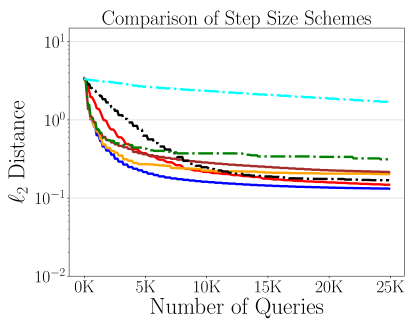
We compare several schemes of choosing step size at each step. The first scheme is suggested by Theorem 1: at the -th step, we set , which we call “Scale with Distance (Sqrt. Decay).” We include the other two scales which scale with distance, “Scale with Distance (Linear Decay)” with and “Scale with Distance (No Decay)” with . We then include “Grid Search,” which searchs step sizes over a log-scale grid, and chooses the step size that best controls the distance with the original sample after projecting the updated sample back to the boundary via binary search. Finally, we include constant stepsizes at . For all schemes, we always use geometric progression to decrease the step size by half until before the next binary search step.
Figure 9 plots the median distance against the number of queries for all schemes. We observe that the scheme suggested by Theorem 1 achieves the best performance in this experiment. Grid search costs extra query budget initially but eventually achieves a comparable convergence rate. When the step size scales with the distance but with inappropriately chosen decay, the algorithm converges slightly slower. The performance of the algorithm suffers from a constant step size.
Choice of perturbation size and introduction of baseline
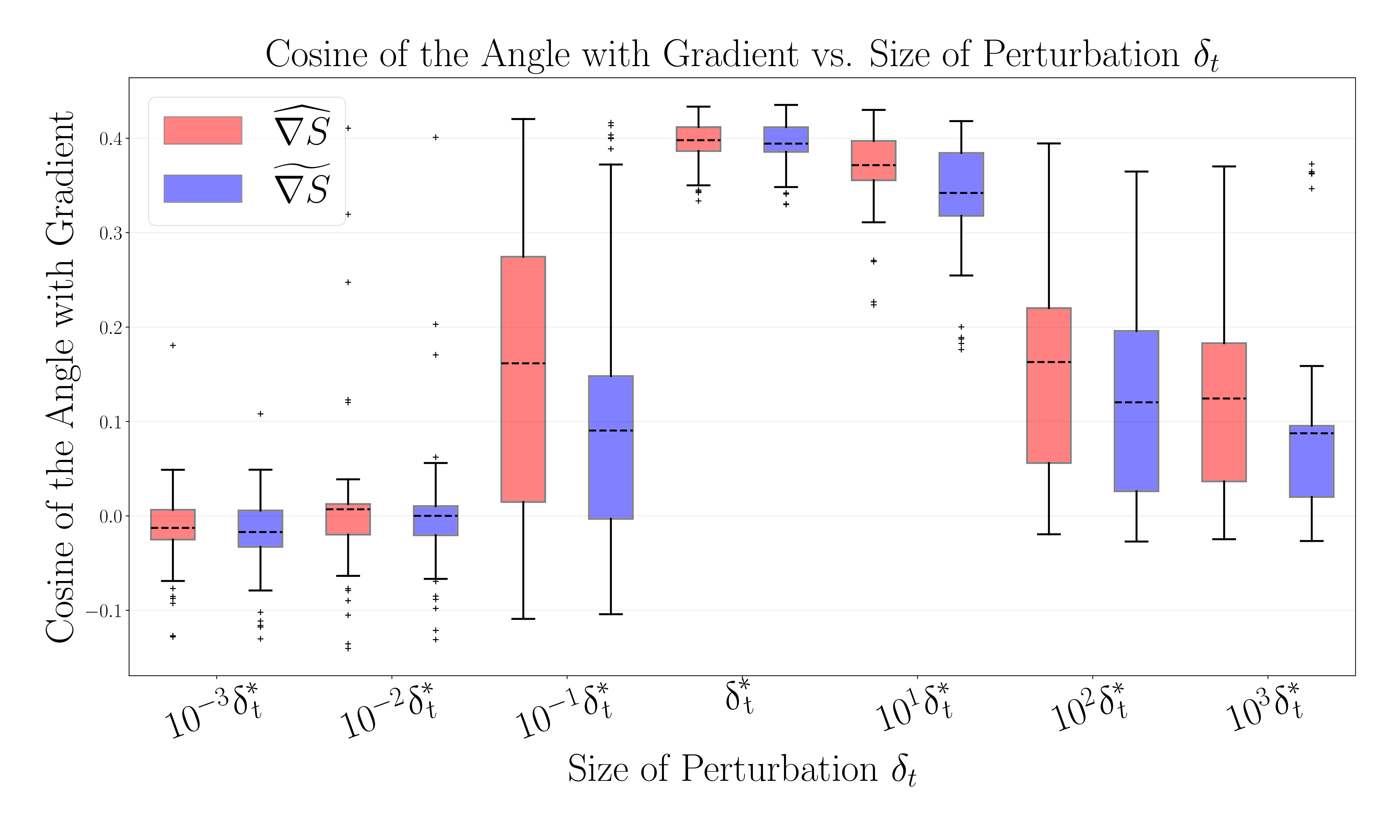
We now study the effectiveness of the proposed perturbation size and baseline for estimating gradient direction when the sample deviates from the boundary. In particular, we focus on the choice of and the introduction of baseline analyzed in Section IV. Gradient direction estimation is carried out at perturbed images at the th iteration, for . We use the cosine of the angle between the gradient-direction estimate and the truth gradient of the model as a metric.
Figure 10 shows the box plots of two gradient-direction estimates as varies among , where is our proposed choice. We observe that our proposed choice of yields the highest cosine of the angle on average. Also, the baseline in further improves the performance, in particular when is not chosen optimally so that there is severe unevenness in the distribution of perturbed images.

Appendix C Model without gradients
In this section, we evaluate HopSkipJumpAttack on a model without gradients. We aim to show HopSkipJumpAttack is able to craft adversarial examples under weaker conditions, such as non-differentiable models, or even discontinuous input transform.
Concretely, we implement input binarization followed by a random forest on MNIST. Binarization transforms an input image to an array of , but transforming all pixels larger than a given threshold to , and all pixels smaller than the threshold to . The algorithm for training random forests applies bootstrap aggregating to tree learners. We implement the random forest with default parameters in scikit-learn [42], using the Gini impurity as split criterion. For each split, randomly selected features are used, where is the number of pixels. We evaluate two random forests with different thresholds for binarization: and . With the first threshold, the model achieves the highest accuracy, , on natural test data. The second threshold yields the most robust performance under adversarial perturbation, with accuracy on natural test data.
For both Boundary Attack and HopSkipJumpAttack, we adopt the same initialization and hyper-parameters as in Section V-A. The original image (with real values) is used as input to both attacks for model queries. When an image is fed into the model by the attacker, the model processes the image with binarization first, followed by the random forest. Such a design preserves the black-box assumption for decision-based attacks. We only focus on untargeted attack here. Note that over of the pixels on MNIST are either greater than or less than , and thus require a perturbation of size at least to change their outputs after being thresholded by . This fact makes perturbation inappropriate for crafting adversarial examples.
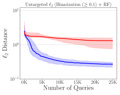
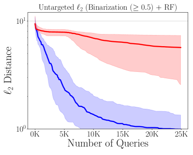

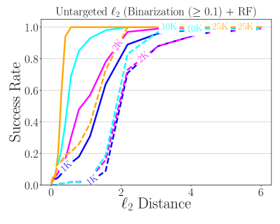
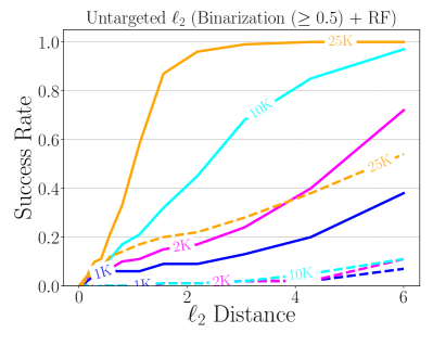

Figure 11 shows the median distance (on a log scale) against the queries, with the first and third quartiles used as lower and upper error bars. Figure 12 shows the success rate against the distance threshold.
When the threshold is set to be , the random forest with binarization becomes extremely vulnerable to adversarial examples. Around adversarial examples fall into the size- -neighborhood of the respective original examples with 1K model queries of HopSkipJumpAttack. The vulnerability is caused by the ease of activating pixels through increasing the strength by . It also indicates HopSkipJumpAttack and Boundary Attack are able to craft adversarial examples without smooth decision boundaries.
When the threshold is set to be , we have a more robust model. A median distance of is achieved by HopSkipJumpAttack through 3K model queries. It takes 25K queries to achieve success rate at an distance of for HopSkipJumpAttack. On the other hand, we observe that Boundary Attack only achieves a median distance of even with 25K model queries. This might result from the inefficiency in spending queries on random walk instead of “gradient direction” estimation step in HopSkipJumpAttack. We remark that the concept of “gradient direction” requires an alternative definition in the current setting, such as a formulation via subgradients.