Diffraction-dominated observational astronomy

Abstract

This paper is based on the opening lecture given at the 2017 edition of the Evry Schatzman school on high-angular resolution imaging of stars and their direct environment. Two relevant observing techniques: long baseline interferometry and adaptive optics fed high-contrast imaging produce data whose overall aspect is dominated by the phenomenon of diffraction. The proper interpretation of such data requires an understanding of the coherence properties of astrophysical sources, that is, the ability of light to produce interferences. This theory is used to describe high-contrast imaging in more details. The paper introduces the rationale for ideas such as apodization and coronagraphy and describes how they interact with adaptive optics. The incredible precision brought by the latest generation adaptive optics systems makes observations particularly sensitive to subtle instrumental biases that must be accounted for, up until now using post-processing techniques. The ability to directly measure the coherence of the light in the focal plane of high-contrast imaging instruments using focal-plane based wavefront control techniques will be the next step to further enhance our ability to directly detect extrasolar planets.

1 Introduction

This edition of the Evry Schatzman school is dedicated to the high angular resolution imaging of the surface of stars and their direct environment. Two families of observational techniques: adaptive-optics (AO) assisted high-contrast imaging and long baseline interferometry, are contributing to making this ambition a reality.

As different as they may seem at first look (see Figure 1), the data produced by these observational techniques share many characteristics. In both cases, whether it be interference fringes or images boosted by a high-order AO system, these data are dominated by diffraction features, that are the combined signature of the telescope and instrumentation used to perform the observations, and include the effect of ever changing atmospheric conditions. The electromagnetic nature of the light collected by the observatory, which can oftentimes be neglected when looking at wide-field images, becomes manifest with these observing techniques since features such as diffraction rings, fringes and speckles become prominent.

For each structure present in the data, one must be able to discriminate the signature of a genuine structure like that of a faint planetary companion, a clump in a circumstellar disk, or a structure of a stellar surface, from a diffraction feature. The ultimate discrimination criterion has to do with the degree of coherence of the structure in question.

Figure 1 presents two examples of diffraction dominated frames, one produced by a single telescope, the other by an interferometer. In both cases, the question one needs to examinate is: is the object I am looking at a point source or did my frame capture the presence of more complex structures? To figure out how to answer this question, we need to take a closer look at the process of image formation.

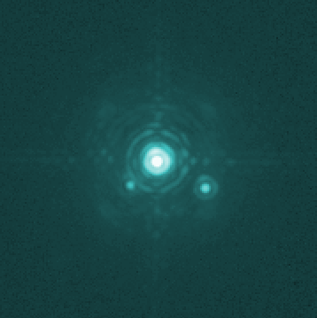
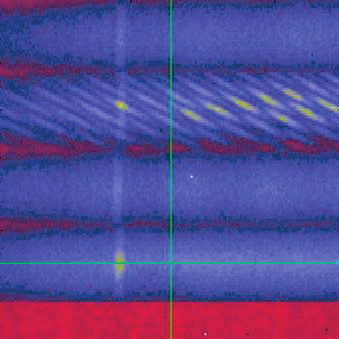
Figure 1: Two examples of diffraction-dominated data: On the left, a K-band AO-corrected image of the binary star $\alpha$-Ophiucus, observed from the Palomar Telescope. On the right, a set of spectrally dispersed two-telescope fringes produced by the instrument AMBER at the focus of VLTI. Both images are dominated by diffraction features such as fringes and rings and can also be affected by other artifacts like ghosts.

2 Images in astronomy

Images are the starting point of a lot of astronomical investigations. Even to the non-expert, because the image is a direct extension of one’s intimate sense of sight, it offers rapid insights into complex situations. The image is the place where an observer will (1) identify new sources, (2) measure their position and brightness relative to a set of references and (3) follow their evolution as a function of time, wavelength and polarization. From these fundamental measurements, populating a multi-dimensional map $I(\alpha,\delta,\lambda,P,t)$ function of position, wavelength, polarization and time, an astronomer will improve his/her understanding (i.e. build a model) of a given object or event, that tells the story of an open star cluster, a group of galaxies, or that of a young planetary system, forming in the vicinity of a nearby star. The fair and efficient interpretation of images is essential to a wide range of scientific applications.

Be it in an actual imaging instrument, a spectrograph or an interferometer, the image is first and foremost, a peculiar optical locus, where the photons coming from a wide number of sources, and more or less uniformly distributed over the collecting surface (the pupil) of one or more telescopes, find themselves optimally segregated by geometric optics. It is possible to describe the result of this photon segregation process as the result $\mathbf{I}$ of a convolution product between two parts: one that is representative of the true distribution of intensities describing the source noted $\mathbf{O}$; and one that describes the instrumental response, that includes the properties of the atmosphere, the telescope and all the optics encountered by the light before reaching the detector. This instrumental response, called point spread function is noted $\mathbf{PSF}$, such that:

$$\mathbf{I}=\mathbf{O}\otimes\mathbf{PSF},$$ (1)

where $\otimes$ represents the convolution operation.

Much effort is devoted by telescope and instrument designers to reduce the impact of the instrumental contribution on the end product. For a great deal of astrophysical observations, the improvement is such that one can directly identify the object $\mathbf{O}$ to the image $\mathbf{I}$ without really paying attention to the $\mathbf{PSF}$. The photon segregation process occuring in the image plane is however fundamentally limited by the phenomenon of diffraction. The scaling parameter that rules this limitation is the ratio between the wavelength of observation $\lambda$ and the characteristic dimension of the aperture used to perform the observation (the diameter of a single telescope, or the length of the interferometric baseline). To quickly estimate the angular resolution provided by a telescope, the following quick formula often comes in handy:

$$\theta\approx 200\times\frac{\lambda}{D},$$ (2)

where $\theta$ is the angular resolution in milli-arcseconds (mas), $\lambda$ the wavelength in microns and $D$ the diameter of the aperture in meters. One can verify that a one-meter telescope observing in the visible ($\lambda=0.5\,\mu$m) offers a 100 mas (0.1”) angular resolution, and that an 8-meter telescope observing in the near-infrared ($\lambda=1.6\,\mu$m) gets down to 40 mas.

Yet even in seemingly ideal observing conditions, the segregation of photons provided by the image is often not sufficient in solving some important problems such as: (1) the identification of faint sources or structures in the direct neighborhood of a bright object: in this context, the faint source one tries to detect is competing for the observer’s attention with the diffraction features of its host or (2) the discrimination of sources of comparable brightness so close to each other that they are said non-resolved. Dealing with these two similar situations is the object of this presentation on diffraction-dominated observational astronomy.

3 Coherence properties of light

Electromagnetic radiation still contributes today to the great majority of the information collected by astronomical observatories that forms the basis of astrophysics: the properties of images produced by astronomical instrumentation can be described using the results of an early XIX^th century physics theory laid out by James Clerck Maxwell. Electromagnetic waves consist of synchronized oscillations of electric and magnetic fields that propagate through a medium at an actual velocity smaller or equal to $c$ (the speed of light through a vacuum). The electric and magnetic fields are orthogonal to one another so that one can specify the wave by keeping track of the electric field alone, which simplifies the description. Note that this presentation will not discuss polarization effects, a refinement that can be added later and won’t change the results and properties derived. Electromagnetic (and therefore electric) waves, are solutions to Helmoltz’s equation (also called the wave equation):

$$\nabla^{2}\mathbf{E}-\frac{1}{c^{2}}\ddot{\mathbf{E}}=0,$$ (3)

where $c$ represents the propagation speed of these waves, i.e. the speed of light. Natural solutions to this equation are oscillating functions with the following form:

$$\mathrm{E}_{\nu}(t,x)=\mathrm{E}_{0}e^{i(kx-\omega t)}=\mathrm{E}_{0}e^{i2\pi(x/\lambda-\nu t)},$$ (4)

characterized by a frequency $\nu$ corresponding to the number of oscillations of the field per seconds (or Hertz) and the wavelength $\lambda$ that corresponds to the distance covered by the propagating electric field over the time of one oscillation. In a vacuum, these two quantities are related via the following inverse relation:

$$\lambda=c/\nu.$$ (5)

The complex exponential form of the oscillating solution of Eq. 4 allows to separate the time and space dependencies of the electric field. The spatial component is awarded a special name: the complex amplitude, noted $A(x)$ such that:

$$\mathrm{E}_{\nu}(t,x)=\mathrm{A}(x)\>e^{-i2\pi\nu t}.$$ (6)

While the complex amplitude is written as the function of a single variable $x$, one has to keep in mind that this complex amplitude is tri-dimensional. Thus if for instance, the origin of the electromagnetic field is a single point source, the electric field is a spherical function of a radius coordinate $r$:

$$\mathrm{E}_{\nu}(t,r)=(1/r)\>\mathrm{E_{0}}e^{i(kr-\omega t)}.$$ (7)

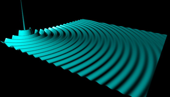
Figure 2: Propagation of a spherical wave. Left: imaginary instant snapshot of the complex amplitude of an electric field emitted by a point source. Directly observing this phenomenon would require a signal commuting time a million time shorter than state of the art fast switching semi-conductors can offer. Right: the static, time-averaged intensity associated to this same electric field, that can indeed be measured in the vicinity of a point source.

The applications covered in this text relate to what is referred-to as the optical: a regime of wavelength that covers the visible, going from $\lambda\sim$ 0.4 $\mu$m to $\lambda\sim$ 0.8 $\mu$m where our human eye is mostly sensitive and the infrared (IR) for wavelengths going up to $\lambda\sim$ 50 $\mu$m. Beyond the infrared, it is customary to use the frequency $\nu$ to describe the electromagnetic radiation. For wavelengths shorter than $\sim$ 100 nm, it is customary to use the energy associated to the radiation. Taking $\lambda=1\mu$m as a wavelength representative of the optical and converting it to a frequency:

$$\nu=\frac{c}{\lambda}=\frac{3\times 10^{8}}{10^{-6}}=3\times 10^{14}\>\mathrm{Hz}.$$ (8)

This really large number explains the specificity of the optical regime. The typical read/write access time of today’s fast switching semi-conductors is of the order of $\sim$ 1 ns. Which means that over the time it takes to switch at least once to take a snapshot, the electric field associated to optical light has oscillated more than $10^{5}$ times. Unlike what is possible in the radio, available readout electronics are not fast enough to record the value of the electric field at any instant (see Figure 2). Instead, one measures the time averaged energy carried by the field and intercepted by a receiver, a quantity called the intensity:

$$I\propto\langle|\mathrm{E}|^{2}\rangle = \int_{t_{0}}^{t_{0}+\tau}\mathrm{E}(t)^{2}\>\mathrm{d}t$$ (9)

$$= |\mathrm{A}|^{2}\>\>(\mathrm{with}\>\tau>>1/\nu).$$ (10)

that is proportional to the square modulus of the complex amplitude. In the absence of perturbations, the intensity recorded is a quantity that is only a function (see Figure 2) of the relative spacing between the source and the observer.

While apparently invisible when considering a single point source, the oscillating nature of the electric field becomes manifest when when a second source is present. The superposition principle states that the solution to this new situation is the sum of the two individual fields. Figure 3 shows what one such field looks like. We still don’t have a receiver fast enough to be able to record the oscillations of the resulting field. The intensity associated to the field (visible in the right panel of Figure 3) however now also features some structure: the intensity oscillates and depending on where the receiver is placed, one can either record a maximum or a minimum of intensity. The distance between two consecutive maxima of intensity will be a function of the ratio between the wavelength $\lambda$ and the distance separating the two sources. Optical interferometry is primarily concerned with the characterization of these structures, refered to as interference fringes.

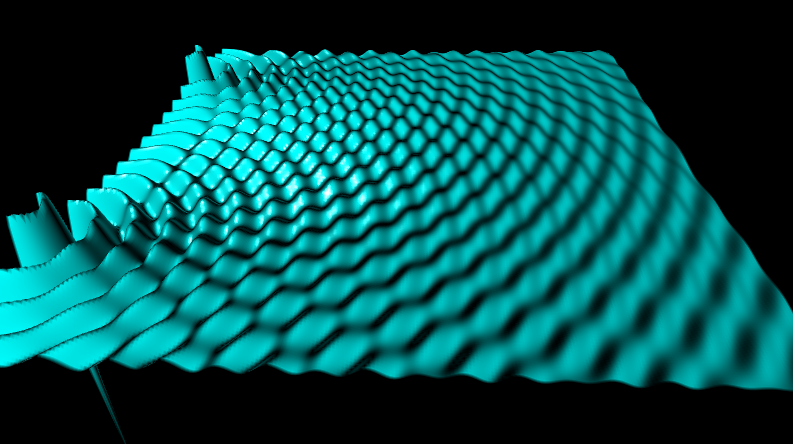
Figure 3: Visualisation of the interference phenomenon. Two point sources, located on the left hand side of the image at the same frequency, both emit a field propagating. Left: The two individual fields add up coherently and produce a rich wave pattern whose periodic properties depend on the frequency of the emission of the sources, and the distance that separates the two sources. Right: the static, time averaged intensity associated to this electric field. Unlike the single source scenario, in the far field (toward the right end of the image), intensity oscillations can be measured along the transverse direction.

This mathematical description of the electromagnetic nature of light would suggest that interference phenomena such as the one that was just described should be commonplace. There are plenty of situations of every day life where the light of two or more sources overlaps on a surface and yet, fringes are a rare occurence. This is because our description has idealized the sources: the purely sinusoidal wave (Eq. 4) is only suited to the description of a laser beam.

The light emitted by thermal light sources like light bulbs or the hot gas of a star originates from a large number of semi-random spontaneous and therefore uncorrelated events like electronic transitions. A more accurate representation of such an emission process uses a series of wave-packets, such as the ones represented in Figure 4, which are a series of damped oscillating fields $E_{k}$ modulated by an envelope function $\mathrm{env}$ and characterized by a random emission time $t_{k}$ and a random phase at origin $\Phi_{k}$:

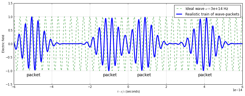
Figure 4: Improved, wave-packet based description of the electric field emitted by a thermal source (solid blue line) compared to the idealized sinusoidal field (dashed green line) used earlier. Random emission times and phase at the origin for each packet result in fluctuations in amplitude and phase of the electric field that will affect its capability to produce interferences.

$$\mathrm{E_{k}}(r,t)=\mathrm{env}(t-{t_{k}})\times e^{i2\pi(r/\lambda-\nu(t-{t_{k}})+{\Phi_{k}})}.$$ (11)

The resulting electric field is no longer purely sinusoidal and fluctuates both in its amplitude and phase: Figure 4 compares this improved wave-packet model to the earlier ideal wave and shows that these fields are no longer synchronized, with the new electric field sometimes ahead of, and sometimes behind the reference. This desynchronization will affect the capacity of the light to produce interferences, a property characterized by a scalar (complex) quantity called the degree of coherence.

The degree of coherence is the result of time-averaged cross-correlation function. It can be used to compare and quantify how look-alike two distinct electric fields are, in which case it will be referred-to as the mutual coherence, or to compare one field with itself delayed in time, which will be referred-to as the self-coherence. This self-coherence is a normalized complex quantity:

$$c(\tau)=\frac{<E^{*}(t)\times E(t+\tau)>}{<|E(t)|^{2}>},$$ (12)

whose modulus $|c(\tau)|\leq 1$. In the case of the ideal wave model, the degree of self-coherence is always equal to one: regardless of the time delay, the electric field will always perfectly interfere with itself delayed in time.

In the wave-packed model, the field is only coherent with itself over when the delay is small. Figure 5 presents two scenarios: a small delay for which the original signal and its copy obviously correlate (ie. look alike); and a large delay (larger than the size of one fringe packet) for which the two fields clearly do not correlate anymore.

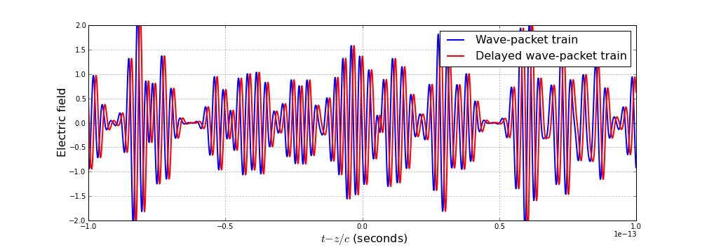
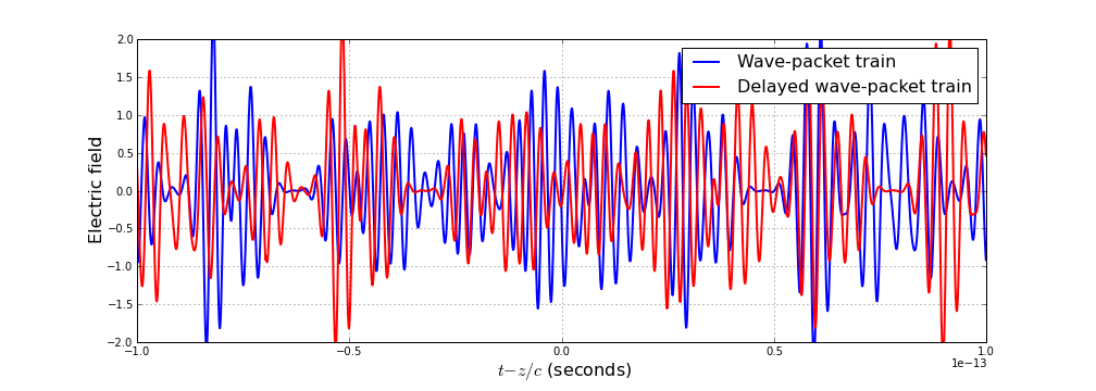
Figure 5: Illustration of the self-coherent properties of an electric field consisting of a collection of wave-packets. Top panel: when the time delay between the two is smaller than the coherence time $\tau_{0}$, the two fields do look alike and the result of their time-averaged cross-correlation exhibits a modulus $c\sim 1$. Bottom panel: beyond the coherence time, the two fields quickly decorrelate and the modulus of their self-coherence reaches $c\sim 0$.

Nevertheless, even ni the second scenario, over a small range of time delays bound by $\tau_{0}$ (the coherence time), one can measure reasonably good correlation between the two signals. If one samples the same field twice, for instance by placing holes in a screen equally distant from a point source, and combines the two fields downstream such that their respective packets reach the same place within the coherence time, interferences can be observed.

When one considers two fields $E_{1}$ and $E_{2}$ emanating from different sources, one uses the degree of mutual coherence:

$$c_{12}(\tau)=\frac{\langle E_{1}(t+\tau)E_{2}(t)^{*}\rangle}{\sqrt{\langle|E_{1}(t)|^{2}\rangle\langle|E_{2}(t)|^{2}\rangle}}=\frac{1}{\sqrt{I_{1}I_{2}}}\int\limits_{\Delta t}E_{1}(t+\tau)E_{2}^{*}(t)\>\mathrm{d}t$$ (13)

to quantify their capacity to interfere with one another. At this point, the reader may have already guessed that two electric fields originating from two distinct series of semi-random events have no chance of being correlated: the expected mutual degree of coherence is equal to zero.

These two elementary observations on the self- and the mutual-coherence of the electromagnetic fields emanating from thermal sources explain all the properties of the formation of image and interference fringes in astronomical instrumentation. Figure 6 offers a graphical summary of these two properties, and leads to the formulation of two simple but very important facts about the light of natural light sources:

• Fact #1: the light emitted by one point source, collected by two or more apertures (or parts of one aperture), and recombined in a manner that all path lengths are equal, will lead to perfect interferences. Unresolved point sources are self-coherent.

• Fact #2: the light from distinct astronomical sources, either distinct objects or two parts of the surface of one object, does not interfere. Astronomical sources are spatially incoherent.

Most of the observing scenarios we are interested in in this lecture focus on a bright, unresolved object that, in most cases, can be treated like a bright point source, surrounded by fainter structures, such as planetary companions, a dust shell or elements of a circumstellar disk.

Figure 6: Self- and spatial-coherence properties of the light emitted by astrophysical sources. Left: The light emitted by one point source, collected by two or more apertures, and recombined in a manner that guarantees that all path lengths are equal (from the source to the detector), will lead to perfect interferences: point sources are self-coherent. Right: The light from distinct astronomical sources, be it two distinct objects or two parts of the surface of one object, does not interfere: astronomical sources are spatially incoherent.

In such a situation, the effective resulting coherence will be dominated by the coherence properties of the bright source, but will be reduced due to the presence of faint sources whose light does not interfere with that of the bright source. The light of a single point source is perfectly coherent: in the case of an interferometer, the estimator of coherence, called the fringe visibility (or the visibility squared), is also equal to one; in the case of a single telescope observation, the image consists of a single, crisp PSF. The presence of additional structures around the bright point source will reduce the apparent visibility of the fringes (in the case of the interferometer) and/or make the single telescope image look fuzzier than on the point source alone: the effective coherence of one such extended source takes intermediate values between 0 and 1.

Being able to measure the coherence of a source from an interferogram or an image assumes that one perfectly knows what the PSF or the fringe pattern acquired on a point source actually looks like. It turns out that several instrumental and environmental effects like the spectral bandpass, atmospheric dispersion, residual aberrations or drifts can result in an apparent loss of coherence. The task is somewhat easier when interpreting a two-aperture interferogram, since the interferometer is really designed to produce unambiguous measurements of coherence, than from an image that contains a complex mix of overlapping spatial frequencies. The deconvolution of images, that is the inversion of Eq. 1, is in practice difficult when the PSF is not perfectly known as the problem is degenerate. We will get back to this very question toward the end of this presentation and see how we can addressit and make our coherence estimates unambiguous.

4 Diffraction-dominated imaging

Since another lecture specifically deals with interferometry, the discussion will from now focus on the properties of images produced by single telescopes. Hopefully, the reader will realize that it doesn’t take long to adapt the following discussion to the case of a multi-aperture interferometer.

Figure 7: Schematic representation of the phenomenon of diffraction. A diaphragm described by the support $\Sigma$, on the left-hand side is uniformly lit by a point source at infinity. The symbols and notations present in this figure are used to determine the distribution of complex amplitude $A(x,y)$ in the right hand side plane located at a distance $Z$ from the diaphragm.

Figure 7 introduces the symbols and the scenario used to describe the phenomenon of diffraction: on the left, a diaphragm or arbitrary shape described by the surface $\Sigma$, uniformly lit by a point source located so far toward the left that (under perfect observing conditions) the complex amplitude of the associated electric field is constant across the aperture. $\Sigma$ describes the aperture of the telescope used to do imaging. If one were to consider looking into interferometry from here, one would just have to split $\Sigma$ into a collection of sub-apertures.

The important relation to establish is one that relates the electric field (at least its complex amplitude) across the aperture $\Sigma$ to its counterpart projected on a screen located at a distance Z from the diaphragm. One elementary surface element d$\sigma$ is singled out on this picture. This elementary surface element is the origin of a new spherical wave (a principle described by Augustin Fresnel in 1818). For a point M of coordinates $(x,y)$ located at a distance r from the origin of the wave, the contribution for the wavelength $\lambda$ to the local complex amplitude from d$\sigma$ is given by:

$$\mathrm{d}A(x,y)=\frac{1}{r}\times K\times A(X,Y)\times e^{j2\pi r/\lambda}\,\mathrm{d}\sigma,$$ (14)

where K is a constant. Since we’ve established that the light associated to a single point source is coherent, we can write that the total electric field in right-hand side plane of Figure 7 is the result of a sum of emissions from all elementary point sources:

$$A(x,y)=K\iint_{\Sigma}\frac{1}{r}\times A(X,Y)\times e^{j2\pi r/\lambda}\,\mathrm{d}\sigma.$$ (15)

If the distance Z between the two diaphragms and the backend screen is sufficiently large in comparison to the dimension of the diaphragm, the distance $r$ can be approximated:

$$r = \sqrt{Z^{2}+(X-x)^{2}+(Y-y)^{2}}$$ (16)

$$\approx Z\biggl{(}1+0.5\biggl{(}\frac{X-x}{Z}\biggr{)}^{2}+0.5\biggl{(}\frac{Y-y}{Z}\biggr{)}^{2}\biggr{)}.$$ (17)

So that the expression for the complex amplitude in the plane on the right hand side of Figure 7 can be rewritten as the result of:

$$A(x,y)=\frac{K}{Z}e^{i2\pi Z/\lambda}\iint_{\Sigma}A(X,Y)\exp{\biggl{(}\frac{i\pi}{\lambda Z}((X-x)^{2}+(Y-y)^{2})\biggr{)}}\,\mathrm{d}\sigma.$$ (18)

This form of integral is called the Fresnel Transform. It is a non-linear transform whose computation can therefore be a bit cumbersome. It is however very general and can be used to compute the diffraction by a diaphragm for a wide range of situations. The Fresnel Transform of Eq. 18 can however be further simplified when the distance $Z$ between the diaphragm and the screen becomes very large, compared to the dimensions of the aperture:

$$\exp{\biggl{(}\frac{i\pi}{\lambda Z}(X-x)^{2}\biggr{)}}\approx\exp{\biggl{(}\frac{i\pi}{\lambda Z}x^{2}\biggr{)}}\times\exp{\biggl{(}\frac{-i2\pi}{\lambda Z}xX\biggr{)}},$$ (19)

when $\frac{X^{2}}{\lambda Z}<<1$. This situation is referred-to as the far field or the Fraunhofer diffraction. While it seems like an approximation, it is perfectly suited to the description of what is happening when a powered optics (see Figure 8) is used to conjugate an object, located at infinity, to its image, placed at a finite distance. In the focal plane of a telescope, the far field approximation becomes perfectly valid. The Fresnel Transform of Eq. 18 can be rewritten as:

Figure 8: The impact of geometric optics on diffraction: a powered optical element conjugates an object located at infinity to an image at a finite distance in the focal plane. To compute the effect of the diffraction by the telescope in the focal plane, one can safely use the Fraunhofer diffraction relying on the computation of Fourier Transforms. To compute the effect of diffraction at any plane located in between the image and the diffractive aperture, one must use the more general Fresnel diffraction.

$$A(x,y)=K^{\prime}\iint_{\Sigma}A(X,Y)\exp{\biggl{(}\frac{-i2\pi}{\lambda F}(xX+yY)\biggr{)}}\,\mathrm{d}\sigma.$$ (20)

where the distance $Z$ has been replaced by the focal length $F$ of the imaging optics. It is convenient to express the coordinates in the image in terms of angular distances relative to the pointing axis, replacing the ratio $x/F$ and $y/F$ by angular coordinates $\alpha,\beta$. One can drop the $K^{\prime}$ constant as well to simplify the notations and just ensure in the computation that the total number of photons collected during an integration, is preserved by the transformation:

$$A(\alpha,\beta)=\iint_{\Sigma}A(X,Y)\exp{\biggl{(}\frac{-i2\pi}{\lambda}(\alpha X+\beta Y)\biggr{)}}\,\mathrm{d}X\mathrm{d}Y.$$ (21)

which you may recognize as the two dimensional Fourier Transform of the distribution of the complex amplitude in the diffracting aperture. Unlike the Fresnel Transform, the Fourier Transform (hereafter represented by the symbol $\mathcal{F}$ is a linear operation that can be computed in an efficient manner. This is the form we will mostly use for the rest of the cases described in this lecture.

Equipped with this quantitative description of the diffraction and our previous observations on the coherent properties of astronomical sources, we can outline a recipe for the formation of an image:

1. an extended source can be described as a finite discrete collection of self-coherent point sources. The object function can be written as $O=\sum_{k}O_{k}$.

2. each point source uniformly illuminates the diffractive aperture. On axis, the complex amplitude ($A_{p}$) is constant. The complex amplitude of each off-axis source includes a phase slope that is proportional to how far off-axis that source is.

3. because each point source is perfectly self-coherent, in the focal plane, the complex amplitude $A_{f,k}$ associated to each point source is the result of the Fourier Transform of the complex amplitude of the field intercepted by the aperture: $A_{f,k}=\mathcal{F}(A_{p,k})$.

4. a detector only records the intensity associated to this point source: $I_{k}=|\mathcal{F}(A_{p,k})|^{2}$. The effect of the phase slope associated to the off-axis source of index $k$ translates the resulting intensity pattern.

5. due to the spatial incoherence property of astronomical sources, the intensity patterns of all point sources add up: $I=\sum_{k}I_{k}$.

Since the light associated to each source is intercepted by the same aperture, the shape of the intensity pattern associated to each source (i.e. the PSF) is the same: the PSF is translation-invariant. It is only modulated by the brightness of individual sources that acts as a scaling factor. The image can therefore be formally described as the weighted sum of PSFs. Figure 9 illustrates this property, which was given as early as Eq. 1 in this presentation but that we can now explain as the direct consequence of the coherence properties of astronomical sources.

Figure 9: The image-object convolution relation illustrated: it is because of the spatial incoherence properties of astronomical sources present in the field (here extracted from a HST/NICMOS image of the Trapezium), that the image can be written as the result of a convolution product between the object function $O$ and the PSF of the telescope and its instrument.

Given the importance of the PSF in the shaping of the final image (see Figure 9), we need to see how the shape and size of the aperture, also known as the pupil, will impact the PSF. The theory of diffraction outlined earlier showed that the PSF can conveniently be computed as the result of the square modulus of the Fourier Transform of the illumination of the pupil:

$$\mathrm{PSF}=\biggl{|}\mathcal{F}(\mathrm{pupil})\biggr{|}^{2}.$$ (22)

Real telescopes unfortunately have fairly complex pupils, featuring at least a central obstruction induced by the presence of a secondary mirror and spider vanes that give support to this secondary mirror. The primary mirror itself can also be made of several segments whose edges induce further diffraction. The PSF of a circular unobstructed telescope (known as the Airy function), only relevant for on-axis refractive telescopes or for an off-axis reflective one, is a useful reference to compare a real telescope to. The circular aperture is one of the few geometries for which the PSF has an analytical expression. Its radial profile is described by:

$$\mathrm{Airy}(r)=4\times\biggl{|}\frac{J_{1}(\pi r)}{\pi r}\biggr{|}^{2},$$ (23)

where $r$ is the angular distance expressed in units of the ratio between the wavelength and the diameter of the aperture ($\lambda/D$) and $J_{1}$ a Bessel function. This Airy pattern, represented in Figure 11 (using a logarithmic scale) features diffraction rings that extend very far away from its core. The Airy function meets its first zero for $r=1.22\lambda/D$, which is often used to estimate the order of magnitude for the angular resolution of an observing setup. Regardless of the details of the aperture, the ratio $\lambda/D$, where $D$ is the characteristic dimension of the diffractive system, will always be the right order of magnitude to consider to characterize the angular resolution of an optical setup. For an 8-meter diameter telescope operating in the near infrared, the ratio $\lambda/D$ is of the order of $\sim 10^{-7}$ radians. Such a small value makes the radian a inconvenient unit to manipulate. In practice, instrument plate scales for imagers at the focus of space-borne or ground based AO-corrected telescopes are usually expressed in milli-arc seconds per pixel. The conversion from radians to arcseconds given by:

$$\theta\>[^{\prime\prime}] = \frac{180\times 3600}{\pi}\times\theta\>[\mathrm{rad}]$$

$$\simeq 206264.8\times\theta\>[\mathrm{rad}],$$

Figure 10: The parsec is the distance at which a projected distance of 1 AU (astronomical unit) corresponds to an angular distance of one arc second. One parsec is therefore roughly equal to $2\times 10^{5}$ AU (see text).

gave us the short-hand formula of Eq. 2 for the angular resolution in mas. The 206,264.8 conversion factor (often rounded to $2\times 10^{5}$) is an order of magnitude that is good to keep in mind. It is indeed the scaling factor between phenomena occuring inside a planetary system (where distances are measured in astronomical units or AU) and phenomena occuring over interstellar distances (for which distances are measured in parsecs). Since the parsec was defined as the distance at which a projected distance of 1 AU corresponds to an angle of one arc second (see Fig. 10):

$$\tan{1^{\prime\prime}}\sim 1^{\prime\prime} = 1\>\mathrm{AU}/1\>\mathrm{pc}$$

$$\theta\>[^{\prime\prime}] = 1/d\>[\mathrm{pc}]$$

$$1\mathrm{pc} = 206264.8\>\mathrm{AU}.$$

5 High-contrast imaging

Figure 11: Left: 2D representation of a the perfect point spread function (PSF) of a circular aperture (using a non-linear color scale). Right: radial profile of the same PSF, over a 10 $\lambda/D$ range of angular separation. Two horizontal lines mark the expected relative brightness (contrast) of two types of planets: self-luminous Jupiter-like at the $10^{-6}$ level and reflective Earth-like at the $10^{-10}$ level. Both lines lay several orders of magnitude below the PSF.

From the rather large sample of extrasolar planets known at the time of this writing, only a dozen systems featuring planetary candidates have been imaged by space-borne and ground-based telescopes. Why is this task so difficult?

For a nearby planetary system, i.e. located $\sim$20 parsecs away from our own Solar system, planets on orbital distances between 1 and 10 AU will appear at angular separations ranging from 50 mas to $0.5^{\prime\prime}$ which seems to be within the angular resolution reach of modern telescopes, even when observing in the near-infrared. The difficulty in the direct imaging of extrasolar planets lies in the very large difference of luminosity between a faint planet and its bright host star. The brightness ratio, also known as the contrast ratio, of a mature Earth-like planet in a 1 AU orbit around an equally mature Sun-like star would be characterized by an incredibly large $10^{-10}$ contrast ratio. A more favorable scenario is that of a self-luminous giant planet like Jupiter in orbit around a young star for which the contrast ratio could stay as high as $10^{-6}$ for a few million years. The right panel of Figure 11 illustrates the difficulty of the situation, by comparing these two scenarios to the ideal PSF profile of a circular aperture. Even at the largest plotted angular separation (10 $\lambda/D$), the signal one would like to detect is still orders of magnitude fainter than the photon noise of the local diffraction structures of the on-axis bright star. When the pupil of the telescope features additional structures such as a central obstruction and spider vanes, the situation is even less favorable.

Simply masking out the PSF in the focal plane does not contribute much: it can help avoid saturation problems on the brightest parts of the PSF but the photon noise of the light present in the diffraction rings will still be the dominant source of noise. To facilitate the detection of faint structures present in the neighborhood of a bright object, one needs to reduce overall on-axis transmission so as to reduce the bright object’s photon noise. The need for high-contrast imaging gave birth to a wide number of techniques amongst which two major families emerge: apodization and coronagraphy. Since the early 2000s, this still active area of research has generated a lot of enthusiasm and become extremely sophisticated. The goal of this presentation is not to give the readers a detailed description of the state of the art, but rather to introduce the important ideas that will help understand how the challenge can be addressed. This will require the application of the diffraction theory that was described earlier.

5.1 Pupil apodization

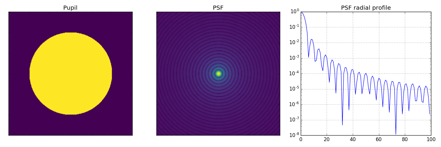
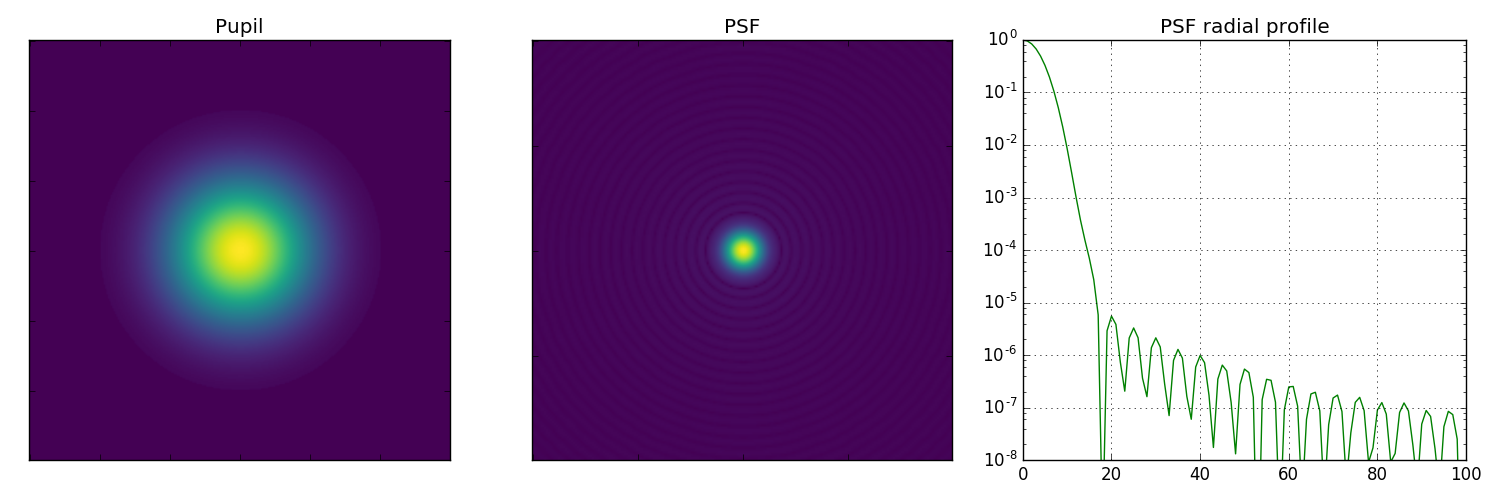
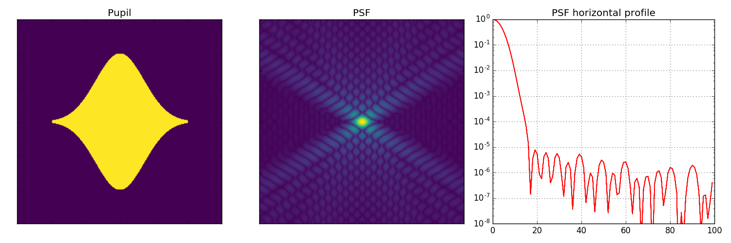
Figure 12: Pupil apodization: the diffraction features of the unobstructed circular aperture (top row) are compared to those produced by two apodization techniques, using either a variable transmission radial mask (middle row) or a binary wave-shaped mask (bottom row). The throughput is reduced from 100 % to $\sim$25 % for the continuous apodization presented in the middle row and to $\sim$56 % for the binary apodization presented in the bottom row. In both cases, the original PSF (top row) is replaced by a PSF better suited to the detection of high-contrast companions. The PSF profiles visible in the right-hand column of panels, using a logarithmic scale, reveal that both apodization approaches can produce PSFs with diffraction features with a contrast that rapidly drops below 10^-5 offering a high-contrast detection advantage over the full aperture for angular separations as low as three resolution elements ($\sim$ 3 $\lambda/D$).

We know that the properties of the PSF of a diffractive aperture are directly related to the Fourier transform of the illumination of that aperture. The diffraction rings observed in the PSF of a circular telescope can be attributed to the sharp transmission edge of the pupil. By tuning the transmission profile of the aperture, one can expect to be able to alter the PSF and its diffraction features. This procedure is referred-to as an apodization and it can result in a PSF featuring no diffraction rings. Figure 12 shows how this apodization effect can be achieved using a fairly simple shaped-pupil mask placed over the original aperture of the telescope. At the cost of some throughput (corresponding to the original aperture surface now covered by the apodization mask), and some angular resolution (the effective aperture size shrinks because of the mask), the PSF features two symmetric dark regions at an orientation that can be adjusted by rotating the apodization mask. The comparison of the PSF profiles represented along the horizontal axis for both apertures shows that the apodization contributes to reducing the brightness of the diffraction by more than two orders of magnitude. The energy previously present in the diffraction rings now contributes to a wider PSF core, of radius $\sim 3\lambda/D$. The size of the new PSF core defines what is now often referred-to as the inner working angle (IWA) of the high-contrast imaging system.

The solution presented here is by no means optimal: the apodization profile chosen to produce these figures follow more or less gaussian shapes. In the litterature, a special class of functions called spheroidal prolates 2003ApJ…582.1147K ; 2003A&A…397.1161S features properties that make them ideal for high-contrast imaging, able to deliver theoretical contrast ratios five orders of magnitude better than those presented in Figure 12. Because the properties of the apodized PSF only depend on the modified pupil shape, the apodized PSF is not more wavelength dependent that its non-apodized counterpart (see the $1/\lambda$ scaling factor in Eq. 21), and will be weakly sensitive to pointing errors. Implemented as it was just described, it however results in throughput and angular resolution loss as it reduces both the effective collective surface area and the effective diameter of the aperture.

Apodization can be achieved using as suggested above, with an aperture mask that suppresses part of the original aperture, or by redistribution of the light which preserves preserves both throughput and resolution 2003A&A…404..379G . The price to pay for one such remapping of the aperture is a PSF that is no longer position invariant (for which the image - object convolution relation of Eq. 1 is no longer valid), at least until that remapping can be undone 2005ApJ…622..744G .

To bring its full benefit, the apodization must be adapted to the features of the aperture Carlotti2011 : the presence of a central obstruction and spider vanes in the pupil would render the simple solutions provided in Fig. 12 useless. The high-performance apodization of real life telescopes is in practice a complex optimization problem requiring a trade-off between IWA, overall transmission, and extinction.

5.2 Coronagraphy

Figure 13: Schematic representation of a coronagraph. The light enters from the left hand side of the diagram and the final (high-contrast) image plane is on the right hand side. The important components of the coronagraph are highlighted in red. From left to right: the apodizer, the focal plane and the Lyot-stop, placed in a relayed pupil. The relay optics (represented by lenses in this diagram) located after the first focus (where the focal plane mask is inserted) are required to form a conjugate pupil plane. The final lense is an imaging optics that produces the final high-contrast image with the appropriate f ratio.

Whereas apodization aims at shaping the PSF so as to reduce the impact of the diffraction rings and spikes, coronagraphy aims at suppressing the light of a bright source from the focal plane. The technique is slightly more complex than straightforward apodization as it requires intervention in at least two optical planes. Figure 13 provides a schematic representation of the elements constituing a coronagraph. Three elements are highlighted in red. Going from left to right, we have: the apodizer that was described earlier, the focal plane mask, located as its name aptly suggests, in the image plane and the so-called Lyot-stop, located in a optical plane that is conjugated with the entrance pupil, after the focal plane mask. While not a part of the original design of the coronagraph, the benefit of apodization described earlier also contributes to improving the coronagraph and both techniques are now used simultaneously Guerri2011 .

The bulk of the light associated to the on-axis bright source (represented in Figure 13 by the left-hand side red dot) encounters the focal plane mask that can either occult it (by absorption or reflection), or dephase it. It was pointed out earlier that masking out the central part of the PSF alone does not result in a suppression of the diffraction features outside of this mask. But if one uses optics to relay the pupil (which is the role of the second lens in the diagram), the use of a second mask, the so called Lyot-stop, completes the effect of the focal plane mask and increases the contrast in the final focal plane. Since it misses the focal plane, the light of an off-axis source (represented by the green dot located next to the star) is almost entirely transmitted by the coronagraph and becomes visible in the final focal plane.

5.3 Coronagraphic formalism

Using our recently acquired diffraction computation skills, we can complete the schematic representation of the coronagraph with a formal description of what is happening at its different stages. Above the different elements represented in Figure 13, a few labels are provided that will be used and referred-to, to describe the complex amplitude of the electric field of starlight going through the coronagraph.

To better distinguish what is taking place in the pupil from what is happening in the focal plane, two sets of coordinates are used: linear $(x,y)$ position coordinates in the aperture and angular $(\alpha,\beta)$ coordinates in the image. The impact of the three elements of the coronagraph is described by the apodizing function $A(x,y)$, the focal plane mask function $M(\alpha,\beta)$ and the Lyot-stop function $L(x,y)$. We now know (see Eq. 21) that a Fourier transform $\mathcal{F})$ relates the complex amplitude in the pupil to the one in the focus: each time the optical system goes back and forth between pupil and image, a Fourier transform is at work. While cumulating the effect of consecutive Fourier transform may sound like a terrible idea at first, it turns out to be fairly simple since:

$$\mathcal{F}(\mathcal{F}(f(x,y)))=f(-x,-y)=\mathcal{R}(f(x,y)),$$ (24)

where $\mathcal{R}$ represents the coordinate flip (or reverse) operator. As long as we don’t land on a detector that records the square modulus of the complex amplitude (see Eq. 10), the elements of the coronagraph directly interact with the local complex amplitude. This interaction is modeled by a multiplication by a complex amplitude gain $g$, with a modulus $0<|g|\leq 1$ (these elements do not amplify the signal) and possibly a phasor $e^{i\phi}$ term if the component introduces a phase delay $\phi$. Another nice property of the Fourier transform that helps understand how the different components affect the final focal plane electric field (and ultimately the intensity), is the convolution property:

$$\mathcal{F}(f(x,y)\times g(x,y))=\mathcal{F}(f(x,y))\otimes\mathcal{F}(g(x,y)),$$ (25)

that says that the Fourier transform of a product is equal to the convolution product of individual Fourier transforms. Thus since the impact of an element of the coronagraph is locally modeled by a multiplication, in the next plane, it results in a convolution.

With these elements in mind, we can finally describe formally what is taking place in the coronagraph, using the following sequence of operations:

• $P_{1}=A$ ($A$ and $P_{1}$ have the same support)

• $F_{1}=\mathcal{F}(P_{1})$ (going to focus $\rightarrow$ Fourier transform)

• $F_{2}=M\times F_{1}$ (focal plane mask multiplies the complex amplitude)

• $P_{2}=\mathcal{F}(F_{2})$ (going back to pupil plane $\rightarrow$ Fourier transform)

  $P_{2}=\mathcal{F}(M\times F_{1})$ (explicit $F_{2}$)

  $P_{2}=\mathcal{F}(M)\otimes\mathcal{F}(F_{1})$ (convolution property)

  $P_{2}=\mathcal{F}(M)\otimes\mathcal{R}(P_{1})$ ($P_{2}=$ input pupil convolved by the mask Fourier-transformed)

• $P_{3}=P_{2}\times L$ (the Lyot-stop blocks parts of the pupil)

• $F_{3}=\mathcal{F}(P_{3})$ (going to final focal plane $\rightarrow$ Fourier Transform)

  $F_{3}=\mathcal{F}(P_{2})\otimes\mathcal{F}(L)$ (convolution property)

  $F_{3}=\mathcal{R}(M\times\mathcal{F}(P_{1}))\otimes\mathcal{F}(L)$ (explicitation of terms)

• $I=|F_{3}|^{2}$ (intensity is square modulus of complex amplitude)

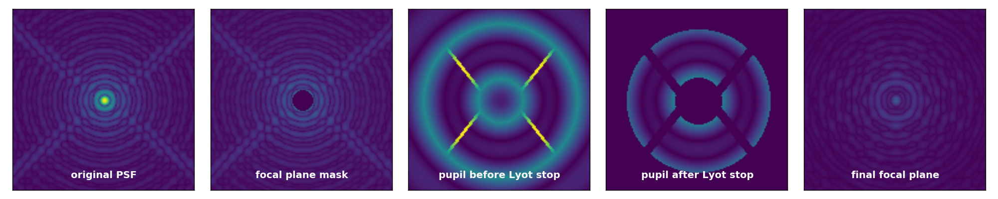
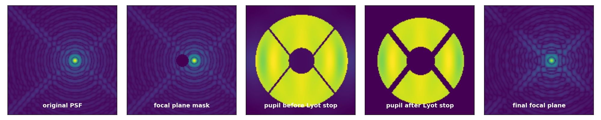
Figure 14: The light going through the differents planes of a coronagraph. The top row shows what happens to an on-axis source, whose primary diffraction lobe will fall within the region occulted by the focal plane mask (second column of panels). The rest of the light is mostly diffracted (in the re-imaged pupil plane) near the edges of the aperture (third columns of panels) and can be suppressed by an undersized Lyot-stop (fourth row of panels). In the final focal plane (fifth column), the light of this on-axis star is considerably attenuated. The second row shows what happens to a source whose primary diffraction lobe misses the focal plane mask.

Figure 14 illustrates these different steps by representing the light of an on-axis (top row) and an off-axis (bottom row) source as it goes through the different planes of a coronagraph, using no apodization and a simple focal plane mask occulting the core of the PSF along with its first Airy ring (radius $\sim 2\lambda/D$). The most important property to observe is the transition from the second to the third column: in the pupil plane that follows the focal plane mask, the light of the on-axis source is no longer uniformly distributed but tends to concentrate near the contours (sharp edges) of the input pupil that features here a central obstruction and spider vanes. To filter this light that would otherwise find its way back to the final focal plane, the Lyot-stop masks out these regions, resulting in a slightly undersized output pupil, with a larger central obstruction and thicker spider vanes. In the final focal plane, the light of this on-axis source is considerably attenuated.

The same operations can be applied to the electric field associated to an off-axis source. The off-axis position will result in a phase slope across the aperture. It it is sufficiently far off-axis (here $\geq\sim 2\lambda/D$), the bulk of this electric field off-axis misses the focal plane. In the output pupil, the light of this source remains mostly uniformly distributed and the Lyot-stop only induces a reduction of the throughput. In the final focal plane, the light of this off-axis source is almost integrally transmitted: the on-axis attenuation combined with a good off-axis transmission results in images revealing faint structures in the bright star’s neighborhood, that would otherwise remain invisible.

The coronagraph used to produce the images of Figure 14 uses an occulting mask, a configuration known as the classical Lyot-coronagraph 1932ZA……5…73L as it replicates (with a smaller occulting mask) the elements that enabled Bernard Lyot to reveal the corona of the Sun in the early 1930s. A review of the litterature will reveal the existence of a wide variety of coronagraphs that use different types of masks that can also induce phase differences 1997PASP..109..815R ; 2003A&A…403..369S , include subwavelength gratings 2005ApJ…633.1191M and feature geometries that split the focus into quadrants 2000PASP..112.1479R ; 2008PASP..120.1112M . The combination of the coronagraph with an apodizer 2005ApJ…618L.161S increases the number of possibilities.

6 Atmospheric turbulence and Adaptive Optics

The purpose of high-contrast imaging devices is to suppress from an image the on-axis static diffraction signature of an optical system that includes the telescope, the beam transfer and the instrument optics. The higher the design performance of the retained solution (often quantified by a level of contrast at a given separation), the more sensitive that solution ends up being to changes in the expected system configuration. One important optical element has however thus far not been taken into consideration: for ground based observations, the atmosphere ends up being a very important element that can quickly wreak havoc on the effective coronagraphic performance. One of the first descriptions of the effect of what we now call atmospheric turbulence can be found as early as 1704 in Isaac Newton’s Opticks:

“If the Theory of making Telescopes could at length be fully brought into Practice, yet there would be certain Bounds beyond which Telescopes could not perform. For the Air through which we look upon the Stars, is in a perpetual Tremor […] The only Remedy is a most serene and quiet Air, such as may perhaps be found on the tops of the highest Mountains above the grosser Clouds.” Book I, Prop. VIII, Prob. II.

The formation of images through a turbulent atmosphere is a complex process, so much that atmospheric optics is a research topic on its own. The three dimensional nature of the atmosphere results in multiple types of degradations: agitation of the image, spreading of the point spread function due to high-order wavefront aberrations and scintillation induced by high altitude turbulence resulting in intensity fluctuations. Figure 15 illustrates the typical effect of turbulence for a 1-meter diameter telescope observing in the visible: the original PSF on the left, with most of the light ($\sim$ 84 %) concentrated over a $\sim 2\lambda/D$ disk is replaced by a random speckle pattern that extends over a much larger area, suggesting the existence of smaller diffractive structures (the atmospheric turbulence cells) Kolmogorov1941 . The typical dimension $r_{0}$ of these cells is called the Fried parameter Fried1966 and the turbulence characteristic evolution time $t_{0}$ depends on the ratio between $r_{0}$ and the velocity $v$ of the turbulent layers. A good observing site is characterized by a large $r_{0}$, meaning that the turbulence is weak and a large $t_{0}$, meaning that it moves slowly. Typical turbulence properties for an average site in the visible ($\lambda$ = 500 nm) are:

• $r_{0}\sim$ 10 cm

• $v\sim$ 10 m/s

• $t_{0}\sim$ 3 ms

What this means is that the high angular resolution potential is no longer just set by the size of the aperture, but also by the properties of that turbulence. In the diffraction scenarios discussed so far, the distribution of complex amplitude for an on-axis source was assumed to be constant across the diffractive aperture: the wavefront was assumed to be perfectly flat. The atmospheric turbulence drastically alters this situation and introduces random phase delays that corrugate the wavefront (see the middle panel of Figure 15 for an example of phase screen).

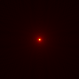
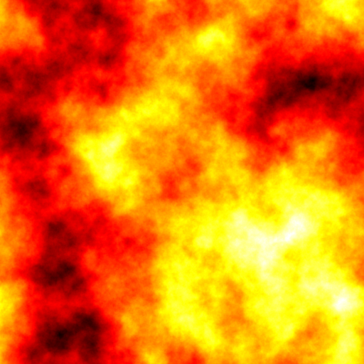
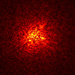
Figure 15: Left: theoretical Airy pattern produced by an unobstructed telescope. Middle: example of Kolmogorov phase screen induced by atmospheric turbulence. Right: instantaneous seeing-limited point spread function experienced when observing through one such atmospheric phase screen.

The structure of the wavefront is not entirely random and is driven by thermodynamics Kolmogorov1941 . One example of Kolmogorov phase screen is represented in the middle panel of Fig. 15. The variance between two parts of the wavefront separated by the distance $\rho$:

$$D_{\Phi}(\rho)=\left<|\Phi_{a}(r)-\Phi_{a}(r+\rho)|^{2}\right>_{r}$$ (26)

is a 2^nd order structure function characterized by one single parameter $r_{0}$ introduced earlier as Fried’s parameter, so that:

$$D_{\Phi}(\rho)=6.88\left(\frac{|\rho|}{r_{0}}\right)^{5/3}.$$ (27)

The power spectrum of the phase deduced for a Kolmogorov phase screen Tatarskii1961 ; Tatarskii1971 :

$$W_{\Phi}(f)=<|\mathcal{F}(\Phi(\rho))|^{2}>=0.0228\>r_{0}^{-5/3}\>f^{-11/3},$$ (28)

shows that the distribution of phase follows a power law with a negative coefficient, which means that the atmosphere introduces more low order aberrations (associated to a low $f$) such as tip-tilt (pointing), focus, astigmatism and coma, than high spatial frequencies. The computation of the diffraction by the aperture (see Eq. 21) is still possible in the presence of turbulence, but the complex amplitude in the aperture $A(X,Y)$ must now include the atmospheric-induced phase delay $\Phi$, so that: $A(X,Y)=e^{i\Phi(X,Y)}$.

The impact of the Kolmogorov phase screen is visible on the right hand side panel of Figure 15 that features a short exposure image that keeps changing with a characteristic time $t_{0}$. One can see that while the PSF spreads out, it is still made of small structures called speckles whose characteristic size remains of the order of $\lambda/D$, suggesting that some high-order spatial frequency content can be recovered from the images if one is able to acquire them with an exposure time of the order of $t_{0}$. This is the object of speckle interferometry 1970A&A…..6…85L ; Aime2001 which won’t be discussed here. A long exposure image through turbulence would wash out these speckles and result in an extended smooth PSF, characterized by a full width half-max of the order of $\lambda/r_{0}$.

Under such observing conditions, a high-contrast imaging device like a coronagraph, originally designed to take out the static component of the aberration, has very little chance of contributing to a contrast improvement in the image. The energy associated to the flux of the bright star, previously concentrated in the central diffraction feature ($\sim$ 84 %) is now spread out over a wide number of fainter speckles. The same thing is also happening to the image of any other source in the field, resulting in an even lower chance of detecting any faint structure near the bright target. Corrective measures have to be taken to restore the wavefront entering the coronagraph and make it as flat as possible again.

Figure 16: Schematic representation of the different elements of a closed-loop adaptive optics-fed imaging system. Starlight enters from the left-hand side of the diagram via the telescope, represented by a single lens. The impact of the atmospheric turbulence is represented by the W-shaped wavefront, that propagates through the system. Relay optics make it possible to project the pupil of the telescope onto a deformable mirror (DM) whose shape can be adjusted to compensate the atmospheric effect on the current wavefront before it feeds the imaging instrument. To determine the shape the DM should take, some light is sampled before the imaging instrument and fed to the wavefront sensor (on the right-hand side of the diagram). The analysis of the information collected by the wavefront sensor will drive a feedback loop that acts on the DM and results in an improved image.

This real-time compensation of the wavefront is the goal of the technique known as adaptive optics (AO). First described in the 1950s Babcock1953 , and deployed by civilian astronomers in the early 1980s Rousset1999 , AO is now a tool available at all major ground based observing facilities that exists in a wide variety of flavors: single or multi-conjugated, involving natural guide stars (NGS) or artificial (laser) guide stars (LGS). For the applications discussed here, AO is used in its simplest possible form: NGS - SCAO. Indeed, because it is focused on a very small field of view (of the order of one arc-second), high-contrast imaging requires single-conjugated adaptive optics (SCAO) and its targets, which are nearby stars, are bright enough to serve as the guide star for the adaptive optics.

An AO system requires two basic functionalities. The first is wavefront control, that is the ability to act on the wavefront of sources present inside the field of view, typically (but not only, as we will see later), to flatten it so as to improve image quality. The second is wavefront sensing, that is the ability to diagnose what is wrong with the current input wavefront, and to determine what can be done in order to correct for it. Figure 16 provides a schematic representation of how these two elements are combined to make up an AO system. It should be pointed out that wavefront sensing can take a wide variety of flavors such as the Shack-Hartmann, the curvature sensor 1988ApOpt..27.1223R or the pyramid sensor Ragazzoni1996 . The ideal wavefront sensor simultaneously combines good sensitivity, ie. the ability to operate on faint guide stars; linearity, ie. the ability to run an unambiguous diagnosis of the wavefront; and a large capture range, ie. the ability to operate in the presence of large or small wavefront errors. Real life sensors all seem to be able to only simultaneously gather two of these qualities at a time 2005ApJ…629..592G , which means that the choice of the wavefront sensor will have consequences on the final outcome. This topic will not be further discussed here and readers interested in this topic are invited to refer to textbooks dedicated to the topic of adaptive optics Roddier2004 ; Hardy1998 . We however need to take a closer look at the wavefront control to be able to understand some important features of AO-corrected images.

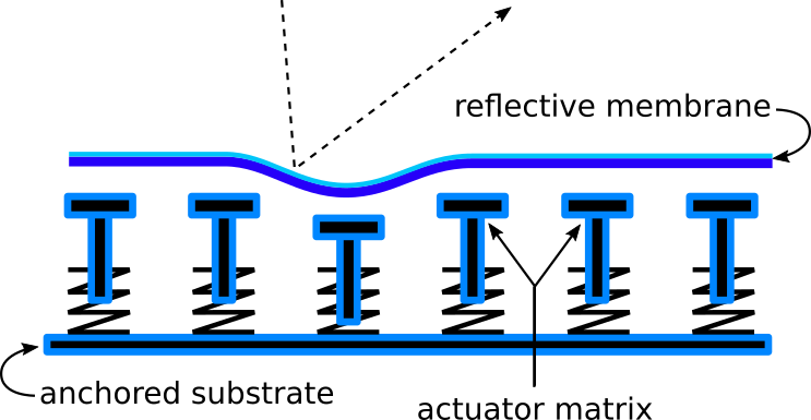
Figure 17: Schematic representation of the layout of a row of actuators pushing or pulling on a continuous reflective membrane. The combined effect of the motion of all actuators gives the ability to generate complex shapes to the deformable surface to compensate the effect of upstream aberrations.

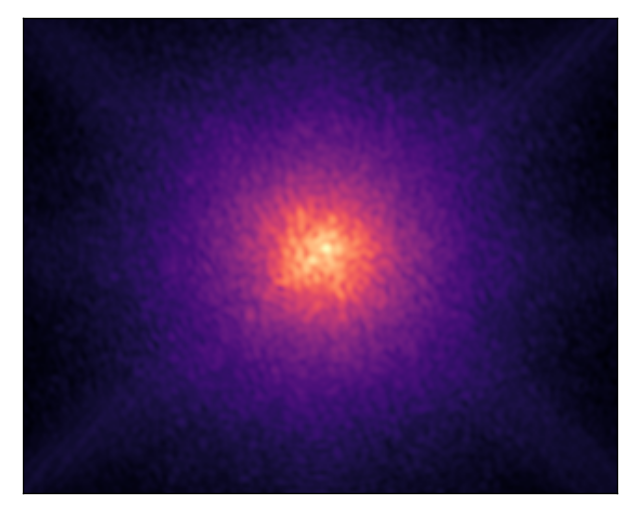
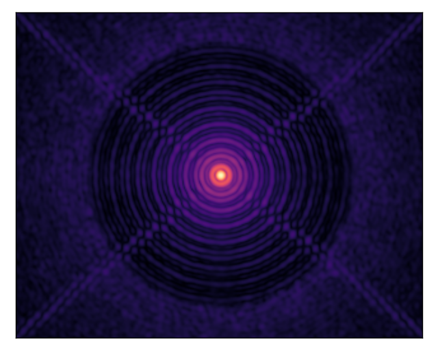
Figure 18: Long exposure acquired through the atmosphere. Left: long exposure acquired in the absence of adaptive optics. Unlike the sharp speckle pattern presented in Fig. 15, the features of this image are washed out by the many turbulence realisations forming a wide halo. Right: long exposure at the focus of an XAO system. The circular region surrounding the now clearly defined and well corrected PSF core at the center of the image marks the domain of spatial frequencies that the DM is able to compensate.

It was shown earlier, that the atmospheric turbulence is characterized by a power spectrum with a -11/3 power law coefficient (see Eq. 28). While the negative sign ensures that less power is contained in the high-spatial frequencies, there is no limit to how fine the turbulence structures get in this description: to correct for everything would require a deformable mirror with an infinite number of active elements, which is not a realistic solution. In practice, a DM is made of a finite number of actuators used either to deform a thin reflective membrane or to push and orient non-deformable mirror segments. For the DMs we are concerned with here, the actuators are laid out on a regular grid. Figure 17 proposes a schematic representation for the implementation of a row of actuators. The total number of actuators distributed across the pupil of the instrument will determine the finesse of the correction one can expect to produce: the DM will act like a filter that can attenuate the atmospheric phase screen up until a cut-off spatial frequency $f_{c}$ imposed by the number of actuators across aperture. For the high-contrast imaging application, the wavefront quality requirement drives the need for a large number of actuators, of the order of a few thousand for an 8-meter aperture. With such a large number of actuators, one sometimes talk about extreme adaptive optics or XAO. The effect of this cut-off spatial frequency is visible in the right panel of Figure 18: a clean circular area surrounds the well corrected PSF core around which one can distinguish the diffraction rings. The DM used to produce this simulated image features $N=50$ actuators across the aperture, pushing the correction radius to $r_{c}=N/2=25\lambda/D$. For an 8-meter aperture observing in the H-band, this translates into a control region that is $\sim$1 arc second. Beyond this correction radius, the power contained in the high-spatial frequency content of the PSF is no-longer compensated and contributes to the formation of another halo.

7 Extreme adaptive optics

The high quality wavefront correction required for high-contrast imaging pushes for AO systems with a large number of actuators, tightly integrated with the coronagraph: the integration of the high contrast imaging constraint to the wavefront control loop marks the specificity of what is now known as extreme adaptive optics. When deforming the mirror, the distribution of complex amplitude $A$ across the aperture of the instrument is given by:

$$A(x,y)=P(x,y)\times e^{i\Phi(x,y)}$$ (29)

where $P(x,y)$ describes the shape of the telescope aperture and $\Phi(x,y)$ the distribution of phase from the combined effect of the atmosphere and the correction by the DM. In the XAO regime, the amplitude of the residual phase is small enough to justify linearizing the complex amplitude:

$$A(x,y)\approx P(x,y)\times(1+i\Phi(x,y)).$$ (30)

Perfect control of the aberrations would mean $\Phi(x,y)=0$ over the entire aperture, leaving only the unity factor resulting in the static diffraction pattern. This linearized form makes it possible to separate the static and the dynamic components of the diffraction, respectively corresponding to the real and imaginary parts of Eq. 30. This form can in turn be used to compute an approximation for the PSF in the low-aberration regime:

$$\mathrm{PSF}(\alpha,\beta)=||\mathcal{F}(P(x,y))||^{2}+||\mathcal{F}(P(x,y)\times\Phi(x,y))||^{2}.$$ (31)

Figure 14 showed how the Lyot-coronagraph manages to attenuate the static diffraction of an on-axis source, but nevertheless leaves a residual: this coronagraph is not perfect. However, other more recent coronagraphic solutions like the vortex 2010ApJ…709…53M and the PIAA 2003A&A…404..379G coronagraphs are closer to being able to completely get rid of this diffraction term 2006ApJS..167…81G . With such designs, the post-coronagraphic residuals for the on-axis source are dominated by the wavefront errors. Coronagraph designs can therefore be benchmarked against the so-called perfect coronagraph, a theoretical design producing the following on-axis coronagraphic image:

$$\mathrm{I}(\alpha,\beta)=||\,\mathcal{F}(P(x,y)\times\Phi(x,y))\,||^{2},$$ (32)

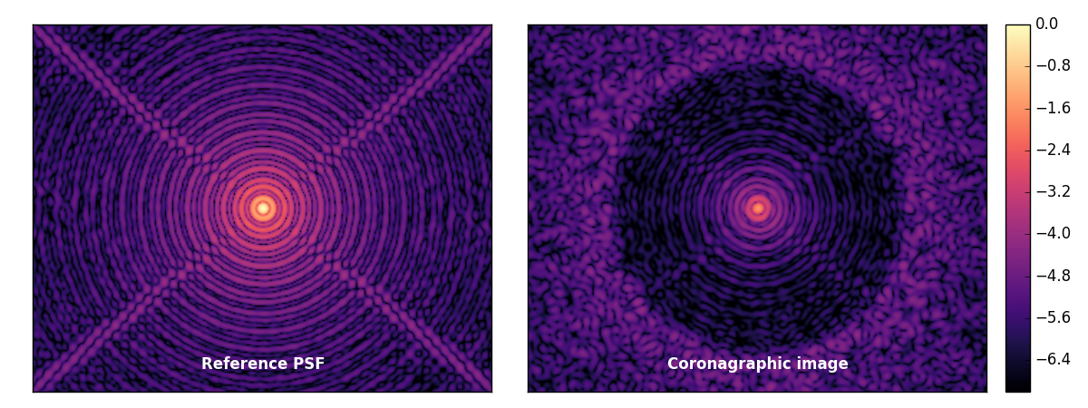
Figure 19: Example of image computation using the perfect coronagraph formula. Left panel: a non-coronagraphic PSF, affected by 50 nm RMS residual wavefront errors. Right panel: a coronagraphic image computed for the same instrument pupil aberration. Both images share the same logarithmic stretch and colorbar.

for which the static diffraction term originally present (see Eq. 31) has deliberately been removed. In the absence of aberrations, the perfect coronagraph provides a perfect extinction of the on-axis source. In the presence of aberrations, the perfect coronagraph leaks and some residual starlight finds its way to the final focal plane. Figure 19 shows one example of application of this perfect coronagraph formula, for an AO-corrected wavefront residual of 50 nm. The details of this computation will depend on the statistics of the residual aberrations. In Eq. 32, we see the phase $\Phi$ squared appearing as a scaling factor for the wavefront aberration residual light in the post-coronagraphic focal plane. A close look at the well-corrected area of the coronagraphic image shown in Fig. 19 shows that the coronagraphic leak does look like a scaled-down copy of the original PSF. For a given RMS level of residuals $\alpha$ (expressed in nanometers) one can therefore predict a focal contrast improvement factor $c_{b}$ (for contrast boost) at any place in the focal plane:

$$c_{b}=\frac{1}{\sqrt{2}}\biggl{(}\frac{2\pi\alpha}{\lambda}\biggr{)}^{2}.$$ (33)

For the simulated 50 nm RMS residual wavefront error shown in Fig. 19, one therefore expects a $c_{b}\approx 0.027$ contrast improvement over the original non-coronagraphic PSF. On Fig. 20, one can verify that over the first $\sim$500 mas of the corrected area, this approximation does match reasonably well the simulated image.

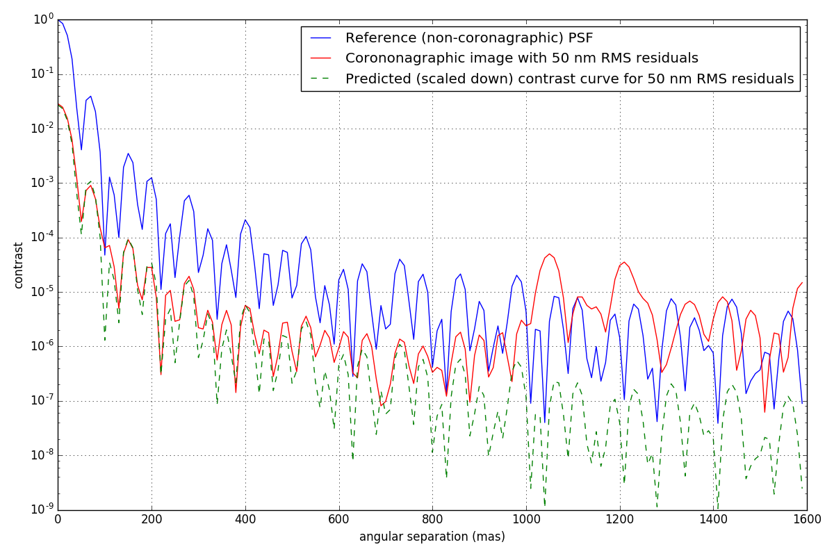
Figure 20: Contrast curves for the perfect coronagraph, in the presence of 50 nm RMS residual wavefront aberration. Three curves are represented, corresponding to radial profiles of the images provided in Fig. 19: the reference (non-coronagraphic) PSF in blue and the corresponding coronagraphic equivalent in red. The green dashed line is a copy of the blue curve, scaled down by the factor $c_{b}$. Over the first $\sim 500$ mas of the plot, the match between the red and the dashed green curves is quite good.

This model can be further refined Herscovici-Schiller2017 and used to derive the statistics of the wave amplitude at each point in the focal plane 2004ApJ…612L..85A , and evaluate the relevance of high-contrast devices in general. What this kind of study shows is that it is not useful to design a coronagraph that attenuates the on-axis PSF of a bright star further than the amount of residual speckles expected for a given amount of residual wavefront aberrations. It is the performance of the AO that will drive how far a coronagraph can help you go, and we will now look into ways the AO performance can unfortunately throw you off target.

8 Calibration of biases

So far, the description has been assuming that the AO system was doing the right thing: to flatten the wavefront so as to help the coronagraph effectively erase the on-axis static component of the diffraction of a bright star. This turns out to be a somewhat naive assumption, due to a simple but fundamental limitation. The wavefront sensor (refer back to Fig. 16) can indeed only sense the aberrations introduced by the instrument optics all the way down to the optics that splits the light between the sensor and the downstream instrument. The AO is therefore understandably oblivious to anything affecting the light on the instrument path after this split which results in practice in a non-common path error. Much care is obviously taken while initially setting up instruments, to minimize any non-common path error however, ground based instruments are not immune to minute temperature changes and mechanical flexures. Given the very strong dependence of the coronagraphic rejection on input wavefront quality, the least amount of non-common path error will considerably reduce the discovery potential of any high-contrast imaging instrument.

These techniques are victims of their own success: before the generalized use of AO, the overall quality of astronomical images produced by a well built instrument was dominated by random atmospheric induced errors. The progressive deployment of AO and the improvement of its performance has reduced the contribution of random errors, resulting in an improved precision. But when the amplitude of random errors is reduced, the effect of small but systematic biases affecting our accuracy become more apparent (see Fig. 21). XAO-fed high contrast imaging and long baseline interferometry make it possible to enter the realm of very high-precision observations: the search and compensation of instrumental biases is becoming more important than ever.

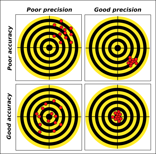
Figure 21: Precision and accuracy are two important statistical concepts that characterize all measurements. As we improve the quality of our instrumentation, usually reducing the precision of the measurements they produce, the impact of systematic bias affecting the accuracy of our conclusions becomes an essential element to take into consideration. Much energy should be spent on understanding the origin of biases and figuring out how to calibrate them out.

Despite the very high quality wavefront control (50 nm RMS only) used to produce the simulated coronagraphic image in Fig. 19, the control region features a large number of speckles amongst which a faint genuine companion to the bright star could hide. If induced by random AO residual errors, the amplitude noise induced by these structures can be reduced simply by accumulating enough data. However if some static or quasi-static speckle structures induced by an aberration that is not seen by the wavefront sensor persist over long time-scales, the detection of faint planetary companions is compromised. We are going back to the important question highlighted in the introduction of this paper: any speckle-like feature present in the image can either be a diffraction induced artefact or a genuine structure of the target being observed.

The non-common path error turns out to be one of the dominant limitations of high-contrast imaging instruments as faint systematic structures are reported to survive in images over timescales stretching as far as $\sim$1 hour. The simplest calibration procedure employed in astronomy consists in using images acquired on a reference object of known characteristics (ideally a featureless single star), observed under conditions as identical as possible to those used for the object of interest, and to subtract the calibration image from the image of the target of interest. Using the shooting analogy used in Fig. 21, we would use a series of shots aiming at the center of the target to figure out how off our aim really is, before going for the big game. This strategy is common for the interpretation of AO-corrected images as well as for optical interferometry for which it is often advised to observe more calibrators than targets of interest.

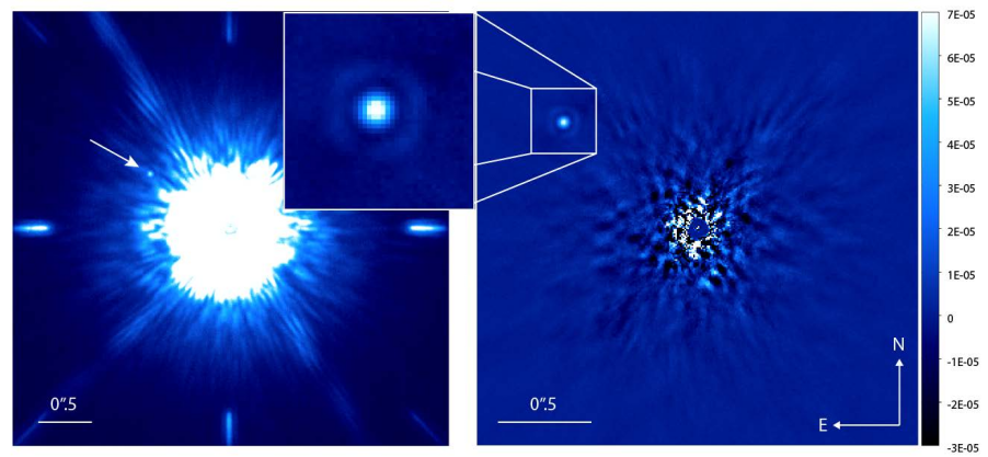
Figure 22: Illustration of the impact of post-processing (from K2018 ) on high-contrast observations with a vortex-coronagraph by the SCExAO instrument 2015PASP..127..890J . The left hand side panel features shows a raw 15 second exposure of $\kappa$-And and the right hand side panel shows the impact of the ADI quasi-static speckle pattern subtraction. The highlighted companion, that could be mistaken for a speckle visible in the raw image, is clearly above the noise level after the post processing has been applied.

While reasonably effective the calibrating potential of this method remains limited: it is difficult to guarantee that observing conditions are indeed strictly identical when going from a science target to a calibrator. The repointing of the telescope, the small differences in elevation, spectral type and evolutions of the atmospheric seeing will eventually translate into biases of their own. For high-contrast imaging, other approaches are available that do not require to alternate observations on a target interest with those of one or more calibration stars: it is indeed possible to take advantage of the field rotation experienced when an instrument is installed at the focus of an alt-azimuthal telescope. When following a target as it transits across the local meridian with one such instrument, the target appears to rotate while the residual diffraction induced by the instrument corrected by the AO but still affected by the non-common path error, remains stable. The relative rotation between the observed scene and the residual diffraction pattern can be used to distinguish spurious diffraction features from genuine structures in a series of images. This approach is referred-to as angular differential imaging or ADI 2006ApJ…641..556M and has led to a wide variety of algorithms such as LOCI 2007ApJ…660..770L . Any type of observation that include some form of diversity such simultaneous imaging in two spectral bands (spectral differential imaging or SDI) or in two polarization states (polarized differential imaging or PDI), theoretically makes it possible to calibrate out systematic effects that bias observations. One must however remain attentive to the implementation details, as these techniques end up relying on further splits of the light path, which can become a source of non-common path. To account for all possible biases during such observations requires a multiple tier calibration procedure, that includes the ability to swap light paths, an example of which is given in Norris2015 .

More recent approaches give a new spin to the idea of using calibrators, by relying on the principal component analysis of a library of reference PSFs Soummer2012 , which provides performance comparable to ADI-inspired approaches. Finally, it is also possible to take the information contained in AO-corrected images (albeit not coronagraphic ones), and to project it onto a sub-space (called the Kernel) that filters out aberrations 2010ApJ…724..464M . The approach is reminiscent of the closure-phase technique used in interferometry 1958MNRAS.118..276J ; 1986Natur.320..595B , but is now applicable to AO-corrected images 2016MNRAS.455.1647P , and is particularly relevant for detection near the diffraction limit (around $\sim$1-2 $\lambda/D$). Regardless of the algorithmic details at work, Figure 22 shows the impact the post-processing has on high-contrast imaging by comparing a single raw coronagraphic image to the result of post-processing of a 10-minute series of images: the impact of the speckle subtraction is spectacular and sometimes contribute as much if not more than the coronagraph itself.

9 Focal-plane based wavefront control?

Unless high-contrast imaging solutions that are intrinsically robust to weak amounts of aberrations do emerge, better calibration stategies must be employed if a performance improvement is desired. The importance for a good calibration of systematic effects in coronagraphic images will grow as the quality of the upstream AO correction keeps on improving. One needs to find, at the level of the focal plane, a discrimination criterion that will make it possible to distinguish a genuine struture in the focal plane from a spurious diffraction induced speckle. The introduction to this paper already hinted at one possibility, relying on the ability to measure the degree of coherence of the structure in question. Section 3 introduced the idea of coherence as the ability of light to interfere. Given the two important coherence properties of astronomical sources: the fact that the light of an unresolved point source is perfectly coherent while the light of distinct point sources is incoherent, can be used to discriminate speckles from planets in an image.

Deliberate modulation of the starlight synchronized with acquisitions by the focal plane camera form the basis for an ideal coherence test that will discriminate the true nature of the high-contrast features present in an image. The deformable mirror can indeed be used to send additional light atop of whatever is currently in the focal plane and the camera can be used to diagnose the degree of coherence of the light recorded in the live image.

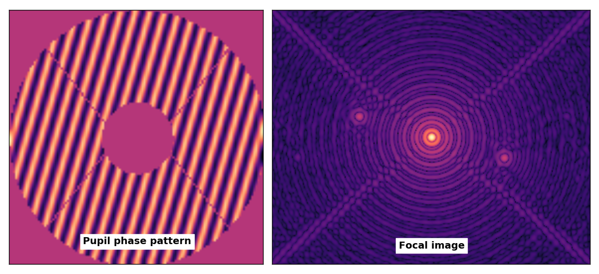
Figure 23: Left: sinusoidal modulation of the wavefront across the instrument pupil by the high-order deformable mirror. Right: the resulting point spread function. The original on-axis diffraction pattern is flanked by two high-contrast replicas at a distance of $\sim$18 $\lambda/D$, given by the number of cycles across the aperture.

The grid structure of the DM actuators (see Figure 17) used in XAO systems makes them particularly suited to the generation of sinusoidal modulation patterns. When one such modulation is applied, the DM behaves like a diffraction pattern and displaces some of the starlight that would otherwise be transmitted on-axis (and possibly attenuated by the coronagraph) at a distance that is proportional to the number of cycles across the aperture.

With $N$ actuators across one aperture diameter, the highest spatial frequency one can reach corresponds to a state where every other actuator is pushed up with the others pushed down: the sinusoidal wave thus generated contains $n_{c}=N/2$ cycles across the aperture. This is what sets the cut-off spatial frequency of AO introduced in Section 6. A deformation $\Delta$ of respectively $k_{x}$ and $k_{y}$ cycles (both $\leq n_{c}$) along the $x$ and $y$ directions of the image is equal to:

$$\Delta(x,y)=a\times\sin(2\pi(k_{x}x+k_{y}y)/D+\phi)$$ (34)

where $a$ is the amplitude of the modulation (typically expressed in microns or nanometers) and $\phi$ the phase of that modulation. For a small modulation amplitude $\alpha$, the complex amplitude $A(x,y)$ induced by this deformation can be linearized (like for Eq. 30):

$$A(x,y) = P(x,y)\times\exp{\biggl{(}i4\pi/\lambda\times\Delta(x,y)\biggr{)}}$$ (35)

$$\approx P(x,y)\times\biggl{(}1+i4\pi a/\lambda\times\sin\bigl{(}2\pi(k_{x}x+k_{y}y)/D+\phi\bigr{)}\biggr{)}$$ (36)

We know that a Fourier transform relates the distribution of complex amplitude in the pupil to that in the focal plane, and can relate values of $a$ and $\phi$ to the properties of speckles in the focal plane. If one knows the Fourier transform of the sine function:

$$\mathcal{F}\bigl{(}\sin{(2\pi kx)}\bigr{)}=\frac{1}{2i}\bigl{(}\delta(u-k)-\delta(u+k)\bigr{)},$$ (37)

where $\delta(u)$ is the Dirac distribution, then the Fourier transform of Eq. 36 will write as:

$$\hat{A}(\alpha,\beta)=\hat{P}(\alpha,\beta)\otimes\biggl{(}\delta(\alpha,\beta)+\frac{2\pi a}{\lambda}\biggl{(}e^{i\Phi}\delta(\alpha-k_{x},\beta-k_{y})-e^{-i\Phi}\delta(\alpha+k_{x},\beta+k_{y})\biggr{)}\biggr{)},$$ (38)

using angular coordinates $\alpha$ and $\beta$ expressed in units of $\lambda/D$. A detector located in the focal plane will record the square modulus of this expression. Each $\delta$ function (convolved by the Fourier transform of the aperture $\hat{P}$) marks the location of one PSF. Eq. 38 therefore allows you to predict that the focal plane will feature two replicas of the original on-axis PSF, at positions given by the number of cycles $k_{x}$ and $k_{y}$. The two replicas are characterized by reference complex amplitudes: $\nu_{1}=(2\pi a/\lambda)\times e^{i\Phi}$ and $\nu_{2}=(2\pi a/\lambda)\times e^{i(\pi-\Phi)}$. An example of image showing this is shown in Fig. 23 for $\sim$18 cycles, resulting in a pair of symmetrical replicas of the on-axis PSF at $\sim$18 $\lambda/D$. Whereas the number of cycles imposes the location of the replicas, the amplitude of the modulation $a$ sets the contrast relative to the original PSF, which is given by:

$$c=(2\pi a/\lambda)^{2}.$$ (39)

Plugging in a sinusoidal phase modulation of amplitude $a=50$ nm therefore produces in the H-band ($\lambda\approx$1.6 $\mu$m) a pair of replicas of contrast $c\approx 4\times 10^{-2}$ which may seem surprisingly bright to the reader. Figure 20 indeed presented for the perfect coronagraph in the presence of a similar level of RMS error, considerably more favorable contrasts. The difference between the two scenarios lies in the structure of the residual phase noise: near random in the case presented in Fig. 20 which distributes the total amount of light associated to the RMS over the control region, or highly structured in the sinusoidal modulation scenario, that focuses the diffracted light onto two specific locations. In addition to the residual RMS given by an AO or XAO system, it is therefore also important to understand how the residuals are distributed across the aperture.

So far, we’ve accounted for the number of cycles $k_{x,y}$ and the modulation amplitude $a$ but not for the $\Phi$ and $\pi-\phi$ phase of the replicas remains: if one were to ignore the convolution operation by $\hat{P}$, taking the square modulus of second term of Eq. 38 would make those phase terms disappear as the $e^{i\Phi}$ factor disappears, suggesting that the phase of the replicas does not matter. The convolution will however bring diffracted light over the area covered by the replica. We have starlight landing atop of starlight: the two contributions will interfere with one another. If the light of an incoherent source is present (ie. a planet or one local disk structure), then the added light will not interfere with this structure: the two intensitise will simply add. Depending on the phase difference between the replica and the speckles or diffraction features already present in the focal plane, the interference can either be constructive or destructive, which leads to an interesting prospect: the possibility of improving the raw contrast of images by tweaking the shape of the deformable mirror. Earlier, it was pointed out that the job of AO feeding a classical imaging system is to flatten the wavefront so as to improve the overall image quality: for a high-contrast imager, the optimal strategy is no longer to flatten the wavefront but to improve the contrast in the focal plane, which can drive the DM to shape the DM quite far from flat. This idea was first envisioned for space 1995PASP..107..386M and has led to a series of sophisticated algorithms such as speckle-nulling 2006ApJ…638..488B , electric field conjugation 2006JOSAA..23.1063G or stroke minimization 2009ApOpt..48.6296P . If the wavefront sensing systems used in modern AO systems tolerate the idea of being driven away from a flat reference wavefront, then this approach becomes implementable on ground based high-contrast imaging instruments.

To produce a fully destructive interference that would result in a local reduction of the local intensity in the image, the complex amplitude of the added replica must match that of the already present structure, with the same amplitude but with opposite phase.

In practice, one does not direcly measure the contrast of speckles: one will primarily access to a local intensity $I_{0}$ which we know will be proportional to the square modulus of the speckle complex amplitude:

$$I_{0}=\gamma\times||a_{0}e^{i\Phi_{0}}||^{2}=\gamma\times||a_{0}||^{2},$$ (40)

where the proportionality constant $\gamma$ will depend on the brightness of the target and the exposure time and will therefore have to be regularly estimated and controlled. While the intensity associated to speckle gives us a proxy for its amplitude $a_{0}$, its phase $\Phi_{0}$ remains unknown. To determine it, one can use a probing approach, which consists in following the evolution of the local intensity as the speckle interferes with a probe speckle of known, stable amplitude $a$ and variable phase $\Phi$. The intensity of the coherent sum of these two complex amplitudes is the result of a classical two-wave interference equation:

$$I(\Phi) = \gamma\times\bigg{|}\bigg{|}a_{0}e^{i\Phi_{0}}+ae^{i\Phi}\bigg{|}\bigg{|}^{2}$$ (41)

$$= \gamma\times\biggl{(}a_{0}^{2}+a^{2}+2a_{0}\>a\cos{(\Phi_{0}-\Phi)}\biggr{)}.$$ (42)

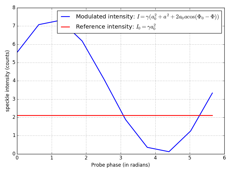
Figure 24: Modulation of the speckle intensity (expressed in units of detector counts) as a function of speckle probe phase. The red curve marks the intensity of the original speckle for which the phase is unknown. The blue curve is the result of the addition of a probe speckle of variable phase $\Phi$. The observed modulation confirms that the speckle is a coherent (ie. contains starlight) structure: one phase of the added speckle ( $\Phi\sim$ 4.5 radians) attenuates the local intensity, resulting in an improved local raw contrast.

This interference function is evaluated for an adaptable number of probes with a phase $\Phi$ uniformly sampled between 0 and 2$\pi$ radians and at least three distinct values of $\Phi$ are required to constrain the values of $a_{0}$ and $\Phi_{0}$. In practice, a finer sampling minimizes the sensitivity to high temporal frequency phase noise (overall jitter and AO dynamic residuals). An example of modulation is represented in Figure 24. It compares the original intensity level marked by the horizontal red line to the blue curve recording the evolution of the phase modulation. When the probe is in phase with the original speckle ($\Phi=\Phi_{0}$), the local intensity is quadrupled. When the probe is in phase opposition with the original speckle ($\Phi=\Phi_{0}+\pi$), the local intensity can be brought to zero.

With four probes, with phases 0, $\pi/2$, $\pi$ and $3\pi/2$, an analytical solution exists to directly measure the complex amplitude of the speckle: this is the so-called ABCD-method. A more general solution is however possible, that is compatible with an arbitrary number $N$ of phases (with $N\geq 3$). It boils down to a parametric model fit of the modulation curve. In addition to $\mathbf{I}_{S}$ the vector of $N$ intensities recorded during the probing sequence, one can precompute a separate vector $\mathbf{W}$ that contains the consecutive powers of the $N^{th}$ root of unity $w_{N}=e^{i2\pi/N}$. The value of the phase $\Phi_{0}$ is directly given by the argument of the dot product between these two vectors:

$$\Phi_{0}=\mathrm{arg}\biggl{(}\mathbf{I}_{S}^{\top}\cdot\mathbf{W}\biggr{)},$$ (43)

while the visibility modulus $\Gamma$ ($0<\Gamma<1$) characterizing the modulation described by Eq. 24 is related to the modulus of the dot product:

$$\Gamma=\frac{2a\>a_{0}}{a^{2}+a_{0}^{2}}=\frac{2}{N}\big{|}|I_{S}^{\top}\cdot W\big{|}|.$$ (44)

The amplitude $a_{0}$ of the original speckle is one of the two roots of the following quadratic equation:

$$a_{0}^{2}-\frac{2a}{\Gamma}a_{0}+a^{2}=0,$$ (45)

which are given by:

$$a_{0}=\frac{a}{\Gamma}\bigl{(}1\pm\sqrt{1-\Gamma^{2}}\bigr{)}.$$ (46)

The amplitude $a$ of the probe is selected to be as close as possible to the amplitude of the speckle $a_{0}$, so as to maximize the visibility modulus $\Gamma$, which results in an improved sensitivity to the properties of the speckle. Because we can’t afford to make a mistake that will amplify the speckle present if we pick the wrong amplitude, one solution is to systematically buff up the probe (for instance by 5 %): some sensitivity is lost but we can be sure that the solution (from Eq. 46) with the minus sign will always be the right one.

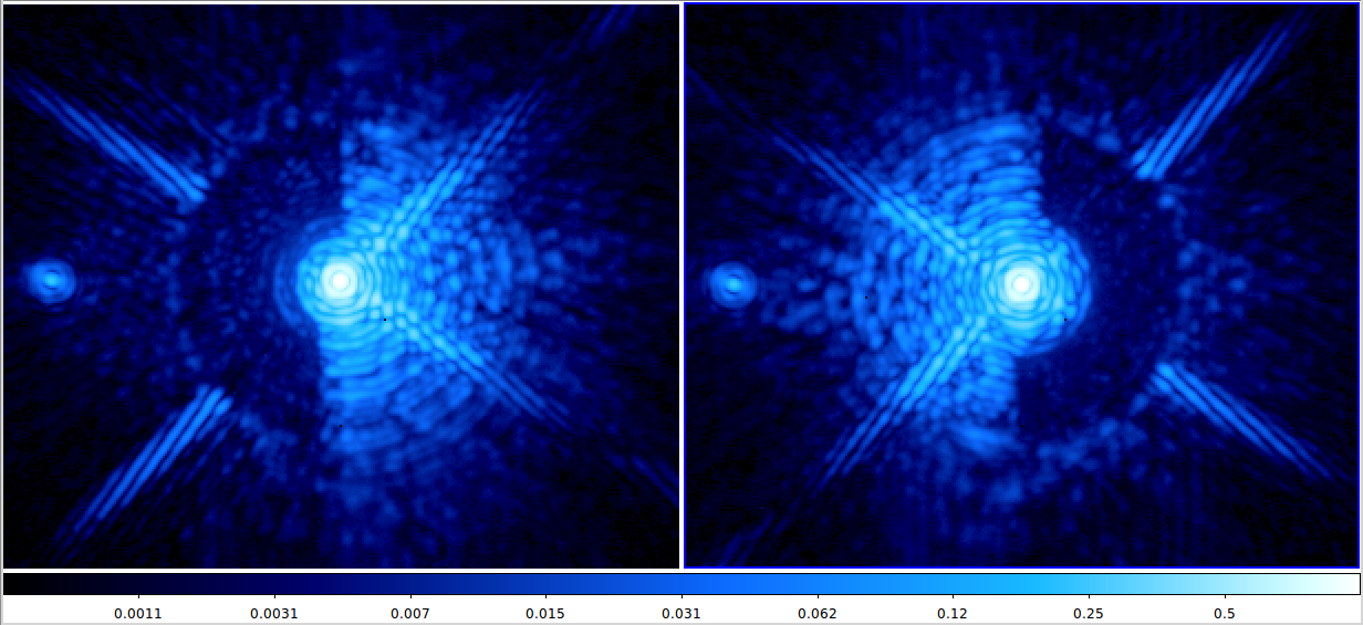
Figure 25: Result of two speckle nulling experiments carried out on the SCExAO instrument on an internal calibration source without a coronagraph. For each image, one can see a high-contrast region was created by the speckle nulling loop on one side of the field of view only. Although it is less obvious on these images, on the opposite side, the speckles and diffraction features of the PSF are amplified as a result of the speckle nulling.

Using this algorithm, it is possible to create a closed-loop focal-plane based wavefront control loop that modifies the reference position of the DM to create a higher contrast area within the control region. Note that while the description of this technique looked at a single speckle, the algorithm can be multiplexed and simultaneously probe dozens or even hundreds of speckles (the exact number depends on the number of actuators available), making it much more efficient. Note that instead of a temporal modulation of the coronagraphic speckle field inside the control region, spatial modulation is possible: the self-coherent camera (SCC) Galicher2008 relies on this idea. Instead of acquiring a sequence of images before applying a correction, the focal plane must be oversampled while a reference beam of starlight is uniformly projected over the control region: the speckles feature fringes that directly encode the complex amplitude properties of the speckles.

Speckles in the focal plane have two origins: they can either be induced by pupil phase aberrations, or can be induced by the geometry of the aperture itself if the coronagraph is absent or if it is imperfect: one can always think of diffraction rings and spikes as being made up of a coherent sum of individual speckles: we can refer to these as induced by pupil amplitude aberrations. It sounds fair game to try and compensate for phase aberration induced speckles by phase modulations, but what of pupil amplitude induced ones? By bending the wavefront, the DM can only redistribute the energy in the focal plane and not make it disappear: when it corrects phase induced speckles, the energy associated to these speckles gets injected back into the original PSF; when it corrects an amplitude induced speckle on one side of the field, it amplifies the speckle on the opposite side. Figure 25 shows the result of two speckle nulling experiments done on the SCExAO instrument in a non-coronagraphic mode. The high-contrast region created by the successive attenuation of speckles covers half of the control region. The appropriate DM modulation produces a high-contrast region in the focal plane, an effect that is similar to what apodization achieves (see Sec. 5.1). The use of static apodizing phase plates achieving a similar effect Kenworthy2007 has been successfully exploited on-sky. These phase plates benefit from advantages that render them fairly achromatic Otten2014 . But like all static high-contrast imaging devices, they are not immune to biases and a focal plane feedback loop remains essential.

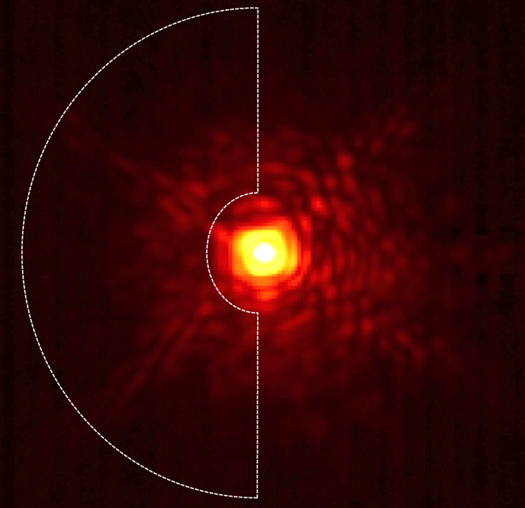
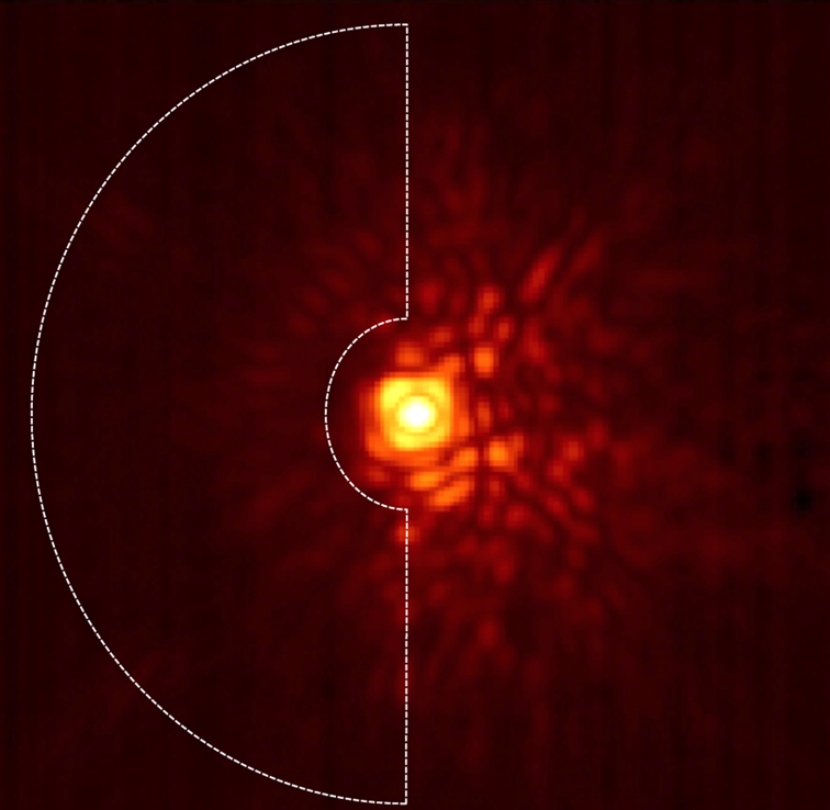
Figure 26: Example of on-sky speckle nulling experiment with the SCExAO instrument without a coronagraph (from 2015PASP..127..890J ). Left: the starting point of the algorithm, after the initial lock of the upstream AO system. Right: after a few minutes of speckle nulling closed loop operation, the left hand side of the field is effectively darker. The D-shaped control region over which the loop is operating is highlighted.

If the same deformable mirror is simultaneously driven by the upstream AO that tends to flatten the wavefront and this focal plane based control that deliberately pushes it away from the flat, to improve the raw contrast in the image, conflicts may occur. One (easy but expensive!) solution may be, in future implementations, to rely on two distinct mirrors for the AO and the high-contrast. The other (cheaper but more difficult) requires the upstream AO system to agree with the idea of stabilizing the wavefront away from flat. This is the object of ongoing work: an exemple of partial speckle nulling correction obtained on sky also with the SCExAO instrument is presented in Figure 26.

10 Conclusion

One of the goals of this lecture was to highlight the formalism and properties that optical interferometry and high-contrast imaging have in common: we first focused on the notion of coherence, most often invoked in the sole context of interferometry, since this technique directly aims at measuring it. The fundamental coherence properties of astronomical sources however also make it possible to explain how images acquired by telescopes form. They also explain what information can be extracted from images dominated by diffraction features. The link between the two techniques runs strong: the Van Cittert Zernike theorem, used at the very heart of interferometry to relate the measurements of complex visibilities to the properties of astrophysical sources (refer to the lecture by Prof. Jean Surdej in this book) can be understood as a Fourier-centric equivalent of the image - object convolution relation.

Equipped with this formal background, we took a closer look at high-contrast imaging and the principles behind the optical techniques of pupil apodization and coronagraphy that attempt to beat down the photon noise of the bright star and improve the detectability of high-contrast sources in their vicinity. We now know that these solutions can only reduce the photon noise associated to the static diffraction figure of the instrumental chain. In the presence of residual aberrations, their performance rapidly degrades and their benefit becomes marginal. State of the art extreme adaptive optics systems, manage to bring the wavefront residual errors down to a few tens of nanometers, but systematic biases, mostly associated to non-common path errors do survive over long time-scales and limit the discovery potential of high-contrast imaging instruments. Sophisticated post-processing techniques do manage to calibrate some of these systematics and have considerably contributed to the direct imaging of a few planetary systems featuring bright planets. There are still orders of magnitude to overcome to directly image the large number of mature planets theoretically within the grasp of ground based telescopes. Before having to resort to post-processing, closed-loop feedback from the focal plane while carrying out the observations seems like a reasonable way to compensate for biases, and design systems that better answer the question: speckle or planet? Going full circle back to the notion of coherence, the example of iterative speckle nulling was described in higher details. Other techniques and algorithms are also possible and may prove more efficient to implement as they mature and adapt to the tough telescope environment. The robustness of the speckle nulling approach however makes it an attractive next step in the elimination of biases for high-contrast imaging.

References

- (1) N.J. Kasdin, R.J. Vanderbei, D.N. Spergel, M.G. Littman, ApJ582, 1147 (2003)
- (2) R. Soummer, C. Aime, P.E. Falloon, A&A397, 1161 (2003)
- (3) O. Guyon, A&A404, 379 (2003), arXiv:astro-ph/0301190
- (4) O. Guyon, E.A. Pluzhnik, R. Galicher, F. Martinache, S.T. Ridgway, R.A. Woodruff, ApJ622, 744 (2005), arXiv:astro-ph/0412179
- (5) A. Carlotti, R. Vanderbei, N.J. Kasdin, Optics Express 19, 26796 (2011)
- (6) G. Guerri, J.B. Daban, S. Robbe-Dubois, R. Douet, L. Abe, J. Baudrand, M. Carbillet, A. Boccaletti, P. Bendjoya, C. Gouvret et al., Experimental Astronomy 30, 59 (2011)
- (7) B. Lyot, ZAp5, 73 (1932)
- (8) F. Roddier, C. Roddier, PASP109, 815 (1997)
- (9) R. Soummer, K. Dohlen, C. Aime, A&A403, 369 (2003)
- (10) D. Mawet, P. Riaud, O. Absil, J. Surdej, ApJ633, 1191 (2005)
- (11) D. Rouan, P. Riaud, A. Boccaletti, Y. Clénet, A. Labeyrie, PASP112, 1479 (2000)
- (12) N. Murakami, R. Uemura, N. Baba, J. Nishikawa, M. Tamura, N. Hashimoto, L. Abe, PASP120, 1112 (2008)
- (13) R. Soummer, ApJ618, L161 (2005), astro-ph/0412221
- (14) A. Kolmogorov, Akademiia Nauk SSSR Doklady 30, 301 (1941)
- (15) D.L. Fried, Journal of the Optical Society of America (1917-1983) 56, 1372 (1966)
- (16) V.I. Tatarskii, Wave Propagation in Turbulent Medium (McGraw-Hill, 1961)
- (17) V.I. Tatarskii, The effects of the turbulent atmosphere on wave propagation (1971)
- (18) A. Labeyrie, A&A6, 85 (1970)
- (19) C. Aime, European Journal of Physics 22, 169 (2001)
- (20) H.W. Babcock, PASP65, 229 (1953)
- (21) G. Rousset, J.L. Beuzit, The COME-ON/ADONIS systems (1999)
- (22) F. Roddier, Appl. Opt.27, 1223 (1988)
- (23) R. Ragazzoni, Journal of Modern Optics 43, 289 (1996)
- (24) O. Guyon, ApJ629, 592 (2005), arXiv:astro-ph/0505086
- (25) F. Roddier, Adaptive Optics in Astronomy (2004)
- (26) J.W. Hardy, Adaptive Optics for Astronomical Telescopes (1998)
- (27) D. Mawet, E. Serabyn, K. Liewer, R. Burruss, J. Hickey, D. Shemo, ApJ709, 53 (2010), 0912.2287
- (28) O. Guyon, E.A. Pluzhnik, M.J. Kuchner, B. Collins, S.T. Ridgway, ApJS167, 81 (2006), arXiv:astro-ph/0608506
- (29) O. Herscovici-Schiller, L.M. Mugnier, J.F. Sauvage, MNRAS467, L105 (2017), 1701.08633
- (30) C. Aime, R. Soummer, ApJ612, L85 (2004)
- (31) J. Kühn, E. Serabyn, J. Lozi, N. Jovanovic, T. Currie, O. Guyon, T. Kudo, F. Martinache, K. Liewer, G. Singh et al., PASP130, 035001 (2018), 1712.02040
- (32) N. Jovanovic, F. Martinache, O. Guyon, C. Clergeon, G. Singh, T. Kudo, V. Garrel, K. Newman, D. Doughty, J. Lozi et al., PASP127, 890 (2015), 1507.00017
- (33) C. Marois, D. Lafrenière, R. Doyon, B. Macintosh, D. Nadeau, ApJ641, 556 (2006), arXiv:astro-ph/0512335
- (34) D. Lafrenière, C. Marois, R. Doyon, D. Nadeau, É. Artigau, ApJ660, 770 (2007), arXiv:astro-ph/0702697
- (35) B. Norris, G. Schworer, P. Tuthill, N. Jovanovic, O. Guyon, P. Stewart, F. Martinache, MNRAS447, 2894 (2015)
- (36) R. Soummer, L. Pueyo, J. Larkin, ApJ755, L28 (2012), 1207.4197
- (37) F. Martinache, ApJ724, 464 (2010), 1009.3933
- (38) R.C. Jennison, MNRAS118, 276 (1958)
- (39) J.E. Baldwin, C.A. Haniff, C.D. Mackay, P.J. Warner, Nature320, 595 (1986)
- (40) B. Pope, P. Tuthill, S. Hinkley, M.J. Ireland, A. Greenbaum, A. Latyshev, J.D. Monnier, F. Martinache, MNRAS455, 1647 (2016), 1510.06406
- (41) F. Malbet, J.W. Yu, M. Shao, PASP107, 386 (1995), arXiv:astro-ph/9502042
- (42) P.J. Bordé, W.A. Traub, ApJ638, 488 (2006), arXiv:astro-ph/0510597
- (43) A. Give’On, N.J. Kasdin, R.J. Vanderbei, Y. Avitzour, Journal of the Optical Society of America A 23, 1063 (2006)
- (44) L. Pueyo, J. Kay, N.J. Kasdin, T. Groff, M. McElwain, A. Give’on, R. Belikov, Appl. Opt.48, 6296 (2009)
- (45) R. Galicher, P. Baudoz, G. Rousset, A&A488, L9 (2008), 0807.2467
- (46) M.A. Kenworthy, J.L. Codona, P.M. Hinz, J.R.P. Angel, A. Heinze, S. Sivanandam, ApJ660, 762 (2007), astro-ph/0702324
- (47) G.P.P.L. Otten, F. Snik, M.A. Kenworthy, M.N. Miskiewicz, M.J. Escuti, Optics Express 22, 30287 (2014), 1412.0660