Interpreting Adversarial Examples by Activation Promotion and Suppression

Abstract

It is widely known that convolutional neural networks (CNNs) are vulnerable to adversarial examples: images with imperceptible perturbations crafted to fool classifiers. However, interpretability of these perturbations is less explored in the literature. This work aims to better understand the roles of adversarial perturbations and provide visual explanations from pixel, image and network perspectives. We show that adversaries have a promotion-suppression effect (PSE) on neurons’ activations and can be primarily categorized into three types: i) suppression-dominated perturbations that mainly reduce the classification score of the true label, ii) promotion-dominated perturbations that focus on boosting the confidence of the target label, and iii) balanced perturbations that play a dual role in suppression and promotion. We also provide image-level interpretability of adversarial examples. This links PSE of pixel-level perturbations to class-specific discriminative image regions localized by class activation mapping (?). Further, we examine the adversarial effect through network dissection (?), which offers concept-level interpretability of hidden units. We show that there exists a tight connection between the units’ sensitivity to adversarial attacks and their interpretability on semantic concepts. Lastly, we provide some new insights from our interpretation to improve the adversarial robustness of networks.

1 Introduction

Adversarial examples are inputs crafted with the intention of fooling machine learning models (?; ?; ?; ?). Many existing works have shown that CNNs are vulnerable to adversarial examples with human imperceptible pixel-level perturbations. Different types of adversarial attacks were proposed with a high success rate of mis-classification. However, understanding these attacks and further interpreting their effects are so far less explored in the literature. In this work, we attempt to study some fundamental questions as follows: a) How to interpret the mechanism of adversarial perturbations at pixel and image levels? b) Rather than attack generation, how to explain the effectiveness of different adversarial attacks? c) How to explore the adversarial effects on the internal response of CNNs? And d) how does the interpretability of adversarial examples help robustness?

		CAM	CAM + perturbed pixels
original image
adversarial image

Figure 1: Explanation of adversarial perturbations produced by the C&W attack (?). The first column shows the original image (with true label ‘Japanese spaniel’) and its adversarial example (with target label ‘bullfrog’). The second column demonstrates CAM of the original image with respect to the true label and CAM of the adversarial example with respect to the target label. At the third column, the adversarial perturbations are overlaid on CAM, and their effects are categorized by our approach: suppression-dominated perturbations (white, at the face of spaniel), promotion-dominated perturbations (black, at the face of bullfrog), and balance-dominated perturbations (gray).

Contributions. First, we study the sensitivity and functionality of pixel-level perturbations on image classification. Unlike adversarial saliency maps (ASMs) (?), our proposed sensitivity measure takes into account the dependency among pixels that contribute simultaneously to the classification confidence. We uncover the promotion-suppression effect (PSE) of adversarial perturbations. We group the adversaries into three types: a) suppression-dominated perturbations that mainly reduce the classification score of the true label, b) promotion-dominated perturbations that focus on boosting the confidence of the target label, and c) balance-dominated perturbations that play a dual role in suppression and promotion.

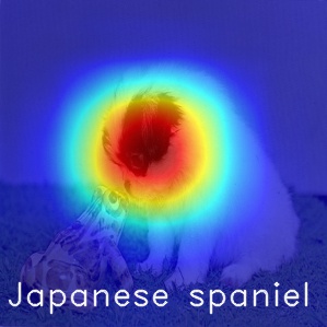
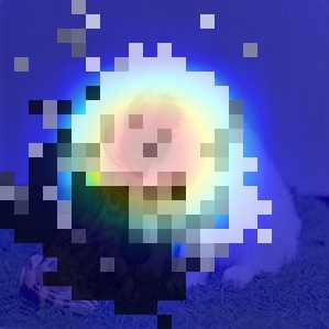
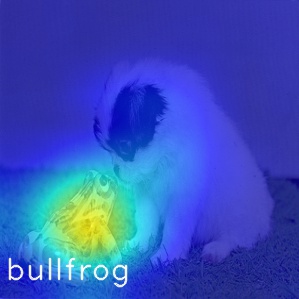
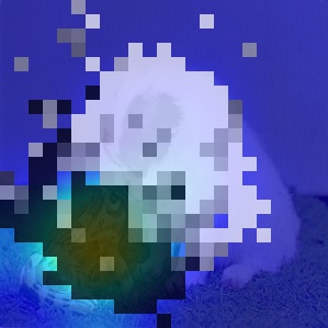
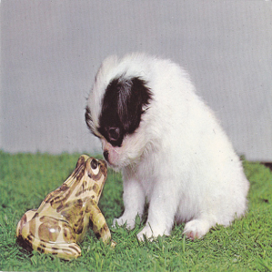
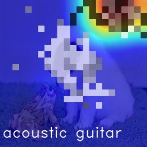
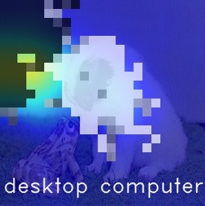
Second, we associate PSE of pixel-level perturbations with image-level interpretability based on class activation map (CAM) (?). We show that the adversarial pattern can be interpreted using the class-specific discriminative image regions. Figure 1 presents an example of the C&W adversarial attack (?), where suppression- and promotion-dominated perturbations are matched to the discriminative regions of the natural image (with respect to the true label ‘Japanese spaniel’) and those of the adversarial example (with respect to the target label ‘bullfrog’), respectively. We also show that the CAM-based image-level interpretability provides a means to evaluate the efficacy of attack generation methods. Although some works (?; ?; ?) attempted to connect adversarial examples with CAM, they mainly focused on the visualization of adversarial examples.

Third, we present the first attempt to analyze the effect of adversarial examples on the internal representations of CNNs using the network dissection technique (?). We show a tight connection between the sensitivity of hidden units of CNNs and their interpretability on semantic concepts, which are also aligned with PSE. Furthermore, we provide some insights on how to improve robustness by leveraging our interpretation of adversarial examples.

Related Works. The effectiveness of adversarial attacks (?; ?; ?; ?; ?; ?) are commonly measured from attack success rate as well as $\ell_{p}$-norm distortion between natural and adversarial examples. Some works (?; ?) generated adversarial attacks by adding unconstrained noise patches, which are different from norm-ball constrained attacks, leading to higher noise visibility. Rather than attack generation, the goal of this paper is to understand and explain the effect of imperceptible perturbations. Here we focus on norm-ball constrained adversarial attacks. Many defense methods have also been developed against adversarial attacks. Examples include defensive distillation (?), random mask (?), training with a Lipschitz regularized loss function (?), and robust adversarial training using min-max optimization (?; ?).

Although the study on attack generation and defense has attracted an increasing amount of attention, interpretability of these examples is less explored in the literature. Some preliminary works (?; ?) were made on evaluating the impact of pixel-level adversarial perturbations on changing the classification results. In (?), Jacobian-based ASM was introduced to greedily perturb pixels that significantly contribute to the likelihood of target classification. However, ASM implicitly ignores the coupling effect of pixel-level perturbations, and it becomes less effective when an image has multiple color channels given the fact that each color channel is treated independently. As an extension of (?), the work (?) proposed an adversarial saliency prediction (ASP) method, which characterizes the divergence of the ASM distribution and the distribution of perturbations.

Both ASM (?) and ASP (?) have helped humans to understand how adversarial perturbations made to inputs will affect the outputs of neural networks, however, it remains difficult to visually explain the mechanism of the adversary given the fact that pixel-level perturbations are small and imperceptible to humans. The work (?; ?) adopted CAM to visualize the change of attention regions of the natural and adversarial images, but the use of CAM is preliminary and its connection with interpretability of pixel-level perturbations is missing. The most relevant work to ours is (?), which proposed an interpretability score via ASM and CAM. However, it focuses on generating structure-driven adversarial attacks by promoting group sparsity of perturbations. In contrast, we provide more thorough and insightful quantitative analysis. In particular, we associate the class-specific discriminative image regions with pixel-level perturbations. We also show that the CAM-based interpretability provides means to examine the effectiveness of perturbation patterns.

From the network perspective, the work (?) investigated the effect of an ensemble attack on neurons’ activations. In (?), Activation Atlas was proposed to show feature visualizations of basis neurons as well as common combinations of neurons. And it was applied to visualizing the effect of adversarial patches (rather than norm-ball constrained adversarial perturbations). Different from (?; ?), we adopt the technique of network dissection (?; ?) to peer into the effect of adversarial examples on the concept-level interpretability of hidden units.

2 Preliminaries: Attack, Dataset, and Model

Let $\mathbf{x}_{0}\in\mathbb{R}^{n}$ denote the natural image, and $\bm{\delta}$ be adversarial perturbation to be designed. Here, unless specified otherwise, the vector representation of an image is used. The adversarial example is then given by $\mathbf{x}^{\prime}=\mathbf{x}_{0}+\bm{\delta}$. By setting the input of the CNNs as $\mathbf{x}_{0}$ and $\mathbf{x}^{\prime}$, the classifier will predict the true label $t_{0}$ and the target label $t$ ($\neq t_{0}$), respectively. To find the minimum adversarial perturbation $\bm{\delta}$ for misclassification from $t_{0}$ to $t$, a so-called norm-ball constrained attack technique is commonly used; Examples considered in this paper include IFGSM (?), C&W (?), EAD (?), and Str attacks (?). We refer readers to Appendix 1 for more details on attack generation.

Our work attempts to interpret adversarial examples from the pixel (Sec. 3), image (Sec. 4) and network (Sec. 5) perspective. At pixel and image levels, we generate adversarial examples from ImageNet under network models Resnet_v2_101 (?) and Inception_v3 (?). At the network level, we generate adversarial examples from the Broadly and Densely Labeled Dataset (Broden) (?), which contains examples with pixel-level concept annotations related to multiple concept categories including color, material, texture, part, scene and object. The considered network model is Resnet_152 (?).

3 Effects of Pixel-level Perturbations

We begin by quantifying how much impact a perturbation could make on prediction confidence. We use the change of logit scores with respect to (w.r.t.) both correct and target labels to measure such an effect. This is in the similar spirit of the C&W attack loss (?) but we focus on grid region-level perturbations as well as the leave-one-out interpretability criterion (?). We build a pixel-level sensitivity measure that can be further used for image-level sensitivity analysis. We aim to answer the questions: How to tag the role of pixel-level perturbations? And how is the perturbation sensitivity associated with the perturbation strength?

Recall that $\mathbf{x}=\mathbf{x}_{0}$ denotes the natural image, and $\mathbf{x}=\mathbf{x}^{\prime}$ corresponds to the adversarial example. We divide an image $\mathbf{x}$ into $m$ grid regions with coordinate sets $\{\mathcal{G}_{i}\}_{i=1}^{m}$, where each $\mathcal{G}_{i}$ contains a group of pixels, and $\cup_{i=1}^{m}\mathcal{G}_{i}=[n]$. Here $[n]$ denotes the overall set of pixels $\{1,2,\ldots,n\}$. We note that a proper size of a grid region facilities visual explanation on semantic image sub-regions and save computation cost. So we set it as $13\times 13$ for ImageNet empirically and also consistent with (?). Let $\bm{\delta}_{\mathcal{G}_{i}}\in\mathbb{R}^{n}$ be the perturbation at the grid region $\mathcal{G}_{i}$, where $[\bm{\delta}_{\mathcal{G}_{i}}]_{j}=\delta_{j}$ if $j\in\mathcal{G}_{i}$, and $0$ otherwise. Here $[\mathbf{a}]_{i}$ or $a_{i}$ denotes the $i$th element of $\mathbf{a}$. We next propose a sensitivity measure of $\bm{\delta}_{\mathcal{G}_{i}}$, which characterizes the impact of pixel-level perturbations on the prediction confidence (in terms of logit score).

Definition 1

(Sensitivity measure of perturbations): The impact of perturbation $\bm{\delta}_{\mathcal{G}_{i}}$ on prediction is measured from two aspects: i) the logit change $d_{0,i}$ w.r.t. the true label $t_{0}$, and ii) the logit change $d_{t,i}$ w.r.t. the target label $t$. That is,

$$d_{0,i}=\max\{Z(\mathbf{x}^{\prime}-\bm{\delta}_{\mathcal{G}_{i}})_{t_{0}}-Z(\mathbf{x}^{\prime})_{t_{0}},\xi\},$$ (1)

$$d_{t,i}=\max\{Z(\mathbf{x}^{\prime})_{t}-Z(\mathbf{x}^{\prime}-\bm{\delta}_{\mathcal{G}_{i}})_{t},\xi\},$$ (2)

$$s_{i}=d_{0,i}+d_{t,i}$$ (3)

for $i\in[m]$, where $Z(\mathbf{x})_{j}$ gives the logit score with respect to class $j$, and $\xi>0$ is a small positive number.

The rationale behind Definition 1 is that the adversarial example $\mathbf{x}^{\prime}$, when it is successfully generated, makes the network misclassified from $t_{0}$ to $t$. Thus, we assign each $\bm{\delta}_{\mathcal{G}_{i}}$ i) the change in the confidence of the true label $t_{0}$ and ii) the change in the confidence of the target label $t$ when $\bm{\delta}_{\mathcal{G}_{i}}$ is removed from the adversarial example $\mathbf{x}^{\prime}$. The sensitivity measure in Definition 1 enjoys the similar spirit of leave-one-out interpretability (?; ?), but the latter focuses on the prediction sensitivity of a single class rather than both $t_{0}$ and $t$.

Figure 2: Illustration on sensitivity measure via the ‘badger’-to-‘computer’ adversarial example generated by C&W attack. Here the true label is ‘badger’ and the target label is ‘computer’. The first column shows the adversarial example and the heat map of $\ell_{2}$-norm distortion at each grid region, i.e., $\{\|\bm{\delta}_{\mathcal{G}_{i}}\|_{2}\}$. The second column presents $\ell_{p}$ norm of $\bm{\delta}_{\mathcal{G}_{i}}$ ($p=2,\infty$), sensitivity scores $d_{0,i}$ and $d_{t,i}$, and PSR $r_{i}$ versus the index of grid regions, where the dash lines correspond to the PSR threshold $\pm 1$.

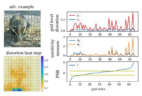
In Definition 1, a large $d_{0,i}$ implies a more significant role of a perturbation $\bm{\delta}_{\mathcal{G}_{i}}$ on suppressing the classification result away from $t_{0}$. By contrast, $d_{t,i}$ measures the effect of $\bm{\delta}_{\mathcal{G}_{i}}$ on promoting the prediction confidence of the target label. The overall adversarial significance $s_{i}$ is the combined effect of $d_{0,i}$ and $d_{t,i}$. Thus, pixels with small values of $s_{i}$ play less significant roles in misleading classifiers. In (1)–(2), we use $\xi$ to get rid of the negative values of $d_{0,i}$ and $d_{t,i}$, i.e., the insignificant cases for the adversary.

With the aid of $\{d_{0,i}\}$ and $\{d_{t,i}\}$ in Definition 1, we define a promotion-suppression ratio (PSR)

$$r_{i}=\log_{2}\left({d_{t,i}}/{d_{0,i}}\right),i\in[m],$$ (4)

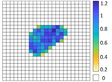
which describes the mechanism of $\bm{\delta}_{\mathcal{G}_{i}}$ on misclassification. In (4), the logarithm is taken for ease of studying PSR under different regimes, e.g, $r_{i}\geq 1$ implies that $d_{t,i}\geq 2d_{0,i}$. Here we categorize the effect of $\bm{\delta}_{\mathcal{G}_{i}}$ into three types. If $r_{i}<-1$, then we call $\bm{\delta}_{\mathcal{G}_{i}}$ a suppression-dominated perturbation, which is mainly used to reduce the classification logit of the true label. If $r_{i}>1$, then we call $\bm{\delta}_{\mathcal{G}_{i}}$ a promotion-dominated perturbation, which is mainly used to boost the classification logit of the target label. If $r_{i}\in[-1,1]$, then we call $\bm{\delta}_{\mathcal{G}_{i}}$ a balance-dominated perturbation that plays a dual role in suppression and promotion. Although different threshold values on $r_{i}$ can be used, we choose $\pm 1$ for ease of visual explanation. In Figure 2 we illustrate the sensitivity measures (1)-(4) through an adversarial example generated by the C&W attack (?). As we can see, either $d_{0,i}$ or $d_{t,i}$ (an thus $s_{i}$) is correlated with the perturbation strength at each grid region (in terms of the $\ell_{p}$ norm of $\bm{\delta}_{\mathcal{G}_{i}}$). Also, PSR implies that most of perturbations in this example contribute to promoting the prediction confidence of the target class. This will also be verified by the image-level interpretability in Figure 4.

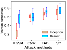
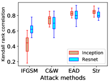
The example of the C&W attack in Figure 2 suggests that the strength of pixel-level perturbations (e.g., in terms of $\ell_{2}$ norm) might be strongly correlated with the input sensitivity scores. For a more thorough quantitative analysis, we examine $5000$ adversarial examples generated by $4$ attack methods under $2$ network models from ImageNet. In Figure 3, we present Pearson correlation and Kendall rank correlation between the distortion strength $\{\|\bm{\delta}_{\mathcal{G}_{i}}\|_{2}\}$ and the proposed sensitivity scores $\{s_{i}\}$ given by (3). We see that C&W, EAD and Str attacks exhibit a relatively stronger correlation than IFGSM since the latter perturbs every pixel due to the use of sign operation, while the former attacks are generated by $\ell_{1}$ and $\ell_{2}$-norm penalized optimization methods that often yield non-uniform and sparser perturbations. For example, the sparest Str-attack has the highest correlation since it perturbs discriminative image regions of high sensitivity (?). In the next section, we will further connect pixel-level perturbations with discriminative image regions.

Figure 3: Correlation between sensitivity scores $\{s_{i}\}$ and $\ell_{2}$ distortion values $\{\|\bm{\delta}_{\mathcal{G}_{i}}\|_{2}\}$. Left: Pearson correlation. Right: Kendall rank correlation.

4 Interpreting Adversarial Perturbations via Class Activation Map (CAM)

CAM (?) and other visual explanation techniques such as GradCAM (?), GradCAM++ (?) and RISE (?) build a localizable deep representation, which exposes the implicit attention of CNNs on a labelled image (?). In this section, we analyze the promotion-suppression effect (PSE) of adversarial perturbations via image-level interpretability. We restrict our analysis to CAM, but can readily be extended to other interpretability methods.

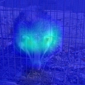
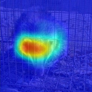
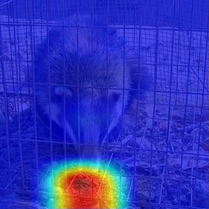
Let $F(\mathbf{x},c)$ denote the CAM for image $\mathbf{x}$ w.r.t. the class label $c$. The strength of a spatial element in $F(\mathbf{x},c)$ characterizes the importance of the activation at this spatial location for classifying $\mathbf{x}$ to the class $c$. Thus, one may wonder the relationship between adversarial examples and discriminative regions localized by CAM. Given natural and adversarial examples, CAMs of our interest include $F(\mathbf{x}_{0},t_{0})$, $F(\mathbf{x}^{\prime},t_{0})$, $F(\mathbf{x}_{0},t)$ and $F(\mathbf{x}^{\prime},t)$ with respect to both the correct and the target labels; see Figure 4 for an example and Figure A2 for more results. Figure 4 suggests that the effect of adversarial perturbations can be visually explained through the class-specific discriminative image regions localized by CAM. Compared $F(\mathbf{x}_{0},t_{0})$ with $F(\mathbf{x}^{\prime},t_{0})$, the most discriminative region w.r.t. $(\mathbf{x}_{0},t_{0})$ is suppressed as $\bm{\delta}$ is added to $\mathbf{x}_{0}$. By contrast, the difference between $F(\mathbf{x}_{0},t)$ and $F(\mathbf{x}^{\prime},t)$ implies that the discriminative region of $\mathbf{x}_{0}$ under $t$ is enhanced after injecting $\bm{\delta}$.

$F(\bm{x}^{\prime},t_{0})$	$F(\bm{x}_{0},t_{0})$	$\mathbf{x}_{0}$	$F(\bm{x}_{0},t)$	$F(\bm{x}^{\prime},t)$
$t_{0}$: badger			$t$: computer

Figure 4: Visualizing CAMs of natural image and its adversarial example (generated by C&W attack) w.r.t. the true label ‘badger’ and the target label ‘computer’, respectively. The heat map color from blue to red represents the least and the most discriminative region localized by CAM, respectively. Here the values of CAMs are normalized w.r.t. the largest value cross CAMs.

We next employ the so-called interpretability score (IS) (?) to quantify how the adversarial perturbation $\bm{\delta}$ is associated with the most discriminative image region found by the CAM $F(\mathbf{x},c)$. More formally, let $B(\mathbf{x},c)$ denote the Boolean map that highlights the most discriminative region,

$$[B(\mathbf{x},c)]_{i}=\left\{\begin{array}[]{ll}1&[F(\mathbf{x},c)]_{i}\geq\nu\\ 0&\text{otherwise},\end{array}\right.$$ (7)

where $\nu>0$ is a given threshold, and $[F(\mathbf{x},c)]_{i}$ is the $i$th element of $F(\mathbf{x},c)$. The IS of adversarial perturbations w.r.t. $(\mathbf{x},c)$ is defined by

$$\mathrm{IS}(\bm{\delta})={\|B(\mathbf{x},c)\circ\bm{\delta}\|_{2}}/{\|\bm{\delta}\|_{2}}.$$ (8)

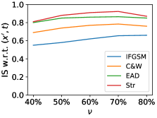
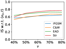
where $\circ$ is the element-wise product. Figure A1 shows the sensitivity of IS against the hyperparameter $\nu$. Not surprisingly, the threshold $\nu$ cannot be too large or too small to highlight the proper discriminative image regions. We set it as $70\%$-quantile of weights in a CAM.

Figure 5: IS under $4$ attack types & $3$ visual explanation methods on Resnet. Left: IS defined on $F(\mathbf{x}_{0},t_{0})$. Right: IS defined on $F(\mathbf{x}^{\prime},t)$. Each box plot represents IS values of $5000$ natural/adversarial examples from ImageNet.

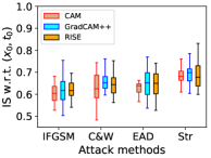
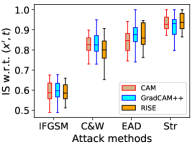
In (8), $\mathrm{IS}(\bm{\delta})\to 1$ if the discriminative region perfectly predicts the locations of adversarial perturbations. By contrast, if $\mathrm{IS}(\bm{\delta})\to 0$, then adversarial perturbations cannot be interpreted by CAM. In Figure 5, we examine IS for $4$ attack types via CAM, GradCAM++ and RISE w.r.t. $(\mathbf{x}_{0},t_{0})$ and $(\mathbf{x}^{\prime},t)$. We see that IS is not quite sensitive to the choice of interpretability methods, since it is built on Boolean localizable maps, which enjoy a large overlapping among different visual explanation tools. We also see that Str and IFGSM yield the best and the worst IS, respectively. These results are consistent with Figure 3: Str-attack tends to perturb local semantic image regions, while IFGSM perturbs every pixel due to the use of sign-based perturbation direction.

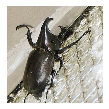
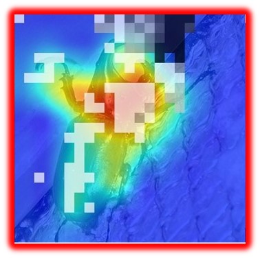
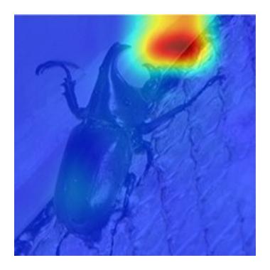
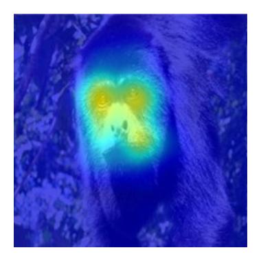
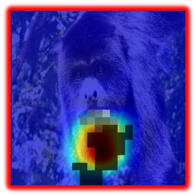
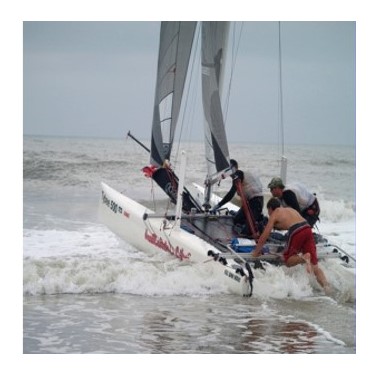
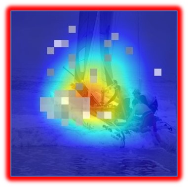
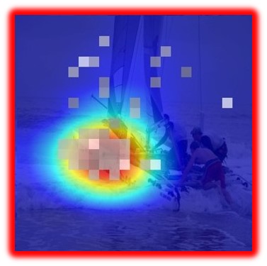
We recall that PSR in (4) categorizes $\{\bm{\delta}_{\mathcal{G}_{i}}\}$ into three types: suppression-dominated perturbations, promotion-dominated perturbations, and balanced perturbations. In Figure 6, we see that the locations and the promotion-suppression roles of adversarial perturbations are well matched to the discriminative regions of $F(\mathbf{x}_{0},t_{0})$ and $F(\mathbf{x}^{\prime},t)$. In particular, if there exists a large overlapping between $F(\mathbf{x}_{0},t_{0})$ and $F(\mathbf{x}^{\prime},t)$, then the balanced perturbations are desired since perturbing a single pixel can play a dual role in suppression and promotion. Toward deeper insights, we investigate how the adversary makes an impact on attacking a single image with multiple target labels (Figure 7) as well as attacking multiple images with the same source and target label (Figure A4). We see that the promotion-dominated perturbation is adaptive to the change of the target label in Figure 7. Moreover, the same source-target label pair enforces a similar effect of adversarial perturbations on attacking different images in Figure A4. Additional results can be found in Appendix 2.

	adv. examples	$F(\bm{x}_{0},t_{0})$ & PSRs	$F(\bm{x}^{\prime},t)$ & PSRs
suppression- dominated effect
	$t_{0}$: rhinoceros beetle – $t$: ambulance
promotion- dominated effect
	$t_{0}$: howler monkey – $t$: paper towel
balance- dominated effect
	$t_{0}$: catamaran – $t$: container ship

Figure 6: Interpreting adversarial perturbations via CAM and PSR. For PSR, only the top $70\%$ most significant perturbed grids ranked by $\{s_{i}\}$ (3) are shown. The white and black colors represent the suppression-dominated regions ($r_{i}<-1$) and the promotion-dominated regions ($r_{i}>1$), respectively. The gray color corresponds to balance-dominated perturbations ($r_{i}\in[-1,1]$). And the red box represents the dominated adversarial effect.

adv. $F(\bm{x}^{\prime},t)$ & PSR adv. $F(\bm{x}^{\prime},t)$ & PSR

Figure 7: Interpreting adversarial examples of the original image ‘Japanese spaniel’ in Figure 1 w.r.t. different target labels ‘acoustic guitar’ and ‘desktop computer’ using CAM and PSR.

Insights on how CAM constrains effectiveness of adversarial attacks. We have previously shown that CAM can be used to localize class-specific discriminative image regions. We now consider two types of CAM-based operations to refine an adversarial perturbation pattern: (a) removing less sensitive perturbations quantified by $s_{i}$ in (3), and (b) enforcing perturbations in the most discriminative regions only w.r.t. the true label, namely, $B(\mathbf{x}_{0},t_{0})$ in (7). We represent the refinement operations (a) and (b) through the constraint sets of pixels $\mathcal{S}_{1}=\{\forall i\,|\,s_{i}>\beta\}$ for a positive threshold $\beta$ and $\mathcal{S}_{2}=\{\forall i\,|\,[B(\mathbf{x}_{0},t_{0})]_{i}>0\}$, where $\beta$ is set to filter perturbations of less than $1-\nu=30\%$ cumulative sensitivity scores. The refined adversarial examples are then generated by performing the existing attack methods with an additional projection on the sparse constraints given by $\mathcal{S}_{1}$ and $\mathcal{S}_{2}$. We refer readers to Appendix 3 for more details.

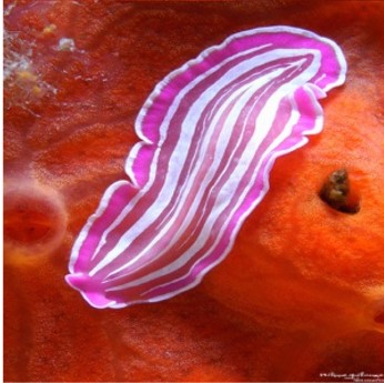
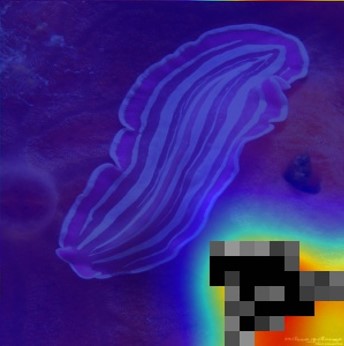
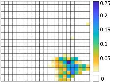
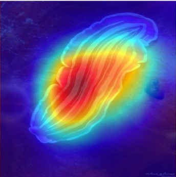
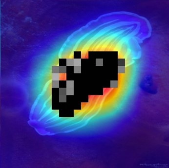
We find that it is possible to obtain a more effective attack by perturbing much less pixels of high sensitivity scores under $\mathcal{S}_{1}$, but without increasing $\ell_{p}$ perturbation strength (Table A1). For attacks with refinement under $\mathcal{S}_{2}$, Figure 8 shows that perturbing pixels under only a suppression-dominated adversarial pattern $\mathcal{S}_{2}$ w.r.t. the true label is not effective: If we restrict perturbations under $\mathcal{S}_{2}$, then the refined attack leads to a much larger $\ell_{2}$ distortion. That is because the perturbation $\bm{\delta}$ originally plays a role in promoting the confidence of the target label, which corresponds to a class-specific discriminative region different from $\mathcal{S}_{2}$.

original	CAM + PSRs w.r.t. adv. image & target label	perturbations (Str-attack)
CAM w.r.t. ori. image & true label	CAM + PSRs w.r.t. refined attack & true label	perturbations (refined Str-attack)

Figure 8: The ‘flatworm’-to-‘knot’ adversarial example (generated by str-Attack) with and without refinement under $\mathcal{S}_{2}$. The first row presents the original image, PSRs overlaid on CAM of the adversarial example w.r.t. the target label ‘knot’, and the $\ell_{2}$-norm distortion of adversarial perturbations. The second row presents $\mathcal{S}_{2}$ given by CAM of the original image w.r.t. the true label ‘flatworm’, and the refined attack under $\mathcal{S}_{2}$. Note that this refinement leads to much larger $\ell_{2}$ distortion (max. value $1.2$) against the unrefined attack (max. value $0.25$); see the third column.

5 Seeing Effects of Adversarial Perturbations from Network Dissection

In this section, we examine the promotion-suppression effect of adversarial perturbations on the internal response of CNNs by leveraging network dissection (?). We show that there exists a connection between the sensitivity of units (a unit refer to a channel-wise feature map) and their concept-level interpretability.

We begin by reviewing the main idea of network dissection; see more details in (?). Interpretability measured by network dissection refers to the alignment between individual hidden units and a set of semantic concepts provided by the broadly and densely labeled dataset Broden. Different from other datasets, examples in Broden contain pixel-level concept annotation, ranging from low-level concepts such as color and texture to higher-level concepts such as material, part, object and scene. Network dissection builds a correspondence between a hidden unit’s activation and its interpretability on semantic concepts. More formally, the interpretability of unit (IoU) $k$ w.r.t. the concept $c$ is defined by (?)

$$\mathrm{IoU}(k,c)=\frac{\sum_{\mathbf{x}\in\mathcal{D}}|\mathbf{M}_{k}(\mathbf{x})\cap\mathbf{L}_{c}(\mathbf{x})|}{\sum_{\mathbf{x}\in\mathcal{D}}|\mathbf{M}_{k}(\mathbf{x})\cup\mathbf{L}_{c}(\mathbf{x})|},$$ (9)

where $\mathcal{D}$ denotes Broden, and $|\cdot|$ is the cardinality of a set. In (9), $\mathbf{M}_{k}(\mathbf{x})$ is a binary segmentation of the activation map of unit $k$, which gives the representative region of $\mathbf{x}$ at $k$. Here the activation is scaled up to the input resolution using bilinear interpolation, denoted by $\mathbf{S}_{k}(\mathbf{x})$, and then truncated using the top $5\%$ quantile (dataset-level) threshold $T_{k}$. That is, $\mathbf{M}_{k}(\mathbf{x})=\mathbf{S}_{k}(\mathbf{x})\geq T_{k}$, namely, the $(i,j)$th element of $\mathbf{M}_{k}(\mathbf{x})$ is $1$ if the $(i,j)$th element of $\mathbf{S}_{k}(\mathbf{x})$ is greater than or equal to $T_{k}$, and $0$ otherwise. In (9), $\mathbf{L}_{c}(\mathbf{x})$ is the input-resolution annotation mask, provided by Broden, for the concept $c$ w.r.t. $\mathbf{x}$. Since one unit might detect multiple concepts, the interpretability of a unit is summarized as $\mathrm{IoU}(k)=(1/|\mathcal{C}|)\sum_{c}\mathrm{IoU}(k,c)$, where $|\mathcal{C}|$ denotes the total number of concept labels.

We next investigate the effect of adversarial perturbations on the internal response of CNNs by leveraging network dissection. We produce adversarial examples $\mathcal{D}^{\prime}$ from Broden using the PGD untargeted attack method (?). Given adversarial examples $\{\mathbf{x}^{\prime}\in\mathcal{D}^{\prime}\}$, we characterize the sensitivity of unit $k$ (to adversarial perturbations) via the change of activation segmentation

$$v(k)\mathrel{\mathop{:}}=\mathbb{E}_{(\mathbf{x},\mathbf{x}^{\prime})}\left[\left\|\mathbf{M}_{k}(\mathbf{x})-\mathbf{M}_{k}(\mathbf{x}^{\prime})\right\|_{2}\right],$$ (10)

where $(\mathbf{x},\mathbf{x}^{\prime})$ is a pair of natural and adversarial examples, and the expectation is taken over a certain distribution of our interest, e.g., the entire dataset or data of fixed source-target labels. In (10), we adopt the activation segmentation $\mathbf{M}_{k}$ rather than the activation map $\mathbf{S}_{k}$ since the former highlights the representative region of an activation map without inducing the layer-wise magnitude bias.

Given the per-unit sensitivity measure $v(k)$ and interpretability measure $\mathrm{IoU}(k)$, we may ask whether or not the sensitive units (to adversarial perturbations) exhibit strong interpretability. To answer this question, we conduct the statistical significance test by contrasting the IoU of the top $N$ ranked sensitive units with the IoU distribution of randomly selected $N$ units. Formally, the $p$-value is the probability of observing $\sum_{k}\mathrm{IoU}(k)$ when $k$ is from top $N$ sensitive units ranked by $v(k)$ in the background IoU distribution when $N$ units are randomly picked. The smaller the $p$-value is, the more significant the connection between sensitivity and interpretability is.

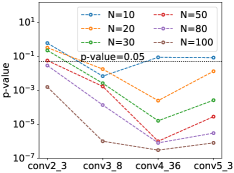
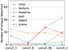
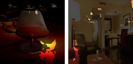
We present the significance test of the interpretability of top $N\in\{10,20,30,50,80,100\}$ sensitive units against the layer index of Resnet_$152$ (Figure 9-a). We also show the number of concept detectors among top $N=100$ sensitive units versus layers for every concept category (Figure 9-b). Here we denote by conv$i\_j$ the last convolutional layer of $j$th building block at the $i$th layer in Resnet_$152$ (?). It is seen from Figure 9-a that there exists a strong connection between the sensitivity of units and their interpretability since $p<0.05$ in most of cases. By fixing the layer number, such a connection becomes more significant as $N$ increases: Most of the top $100$ sensitive units are interpretable, although the top $10$ sensitive units might not be the same top $10$ interpretable units. By fixing $N$, we observe that deep layers (conv4_36 and conv5_3) exhibit stronger connection between sensitivity and interpretability compared to shallow layers (conv2_3 and conv3_8). That is because the change of activation induced by adversarial attacks at shallow layers could be subtle and are less detectable in terms of interpretability. Indeed, Figure 9-b shows that more high-level concept detectors (e.g., object and part) emerge in conv4_36 and conv5_3 while low-level concepts (e.g., color and texture) dominate at lower layers.

(a) (b)

Figure 9: Sensitivity and interpretability. (a) $p$-value of interpretability of top $N$ sensitive units to adversarial attacks in Resnet_$152$, where the presented layers include conv2_3 (256 units), conv3_8 (512 units), conv4_36 (1024 units) and conv5_3 (2048 units). (b) Number of concept detectors among top $N=100$ sensitive units per layer for each concept category.

conv2_3 conv3_8 conv4_36 conv5_3 Ori: table lamp ($t_{0}$) Adv: studio couch ($t$) unit193, orange-color unit358, flecked-texture unit457, shade-part unit1716, lamp-object unit123, sofa-object Ori: airliner ($t_{0}$) Adv: seashore ($t$) unit84, blue-color unit445, banded-texture unit2, stern-part unit781, airplane-object unit782, beach-scene

Figure 10: Visualizing impact of original (Ori) & adversarial (Adv) examples on the response of concept detectors identified by network dissection at $4$ representative layers in Resnet. (top) attack ‘table lamp’-to-‘studio couch, day bed’, (bottom) attack ‘airliner’-to-‘seashore, seacoast’. In both top and bottom sub-figures, the first row presents unit indices together with detected top ranked concept labels and categories (in the format ‘concept label’-‘concept category’). The last two rows present the response of concept detectors visualized by the segmented input image, where the segmentation is given by $\mathbf{M}_{k}(\mathbf{x})$ corresponding to the top ranked concept at each unit.

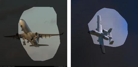
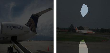
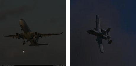
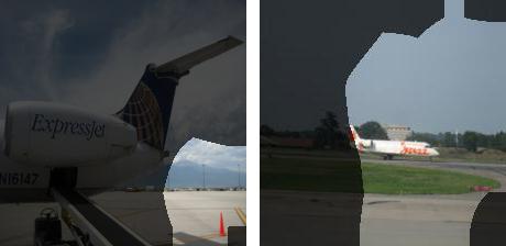
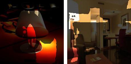
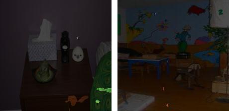
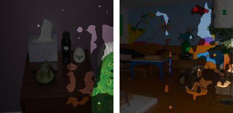
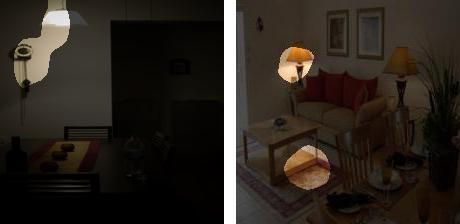
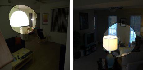
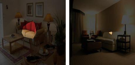
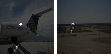
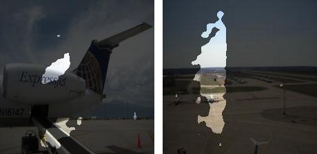
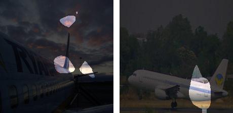
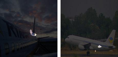
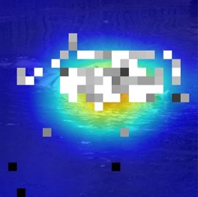
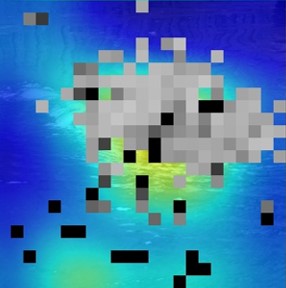
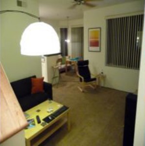
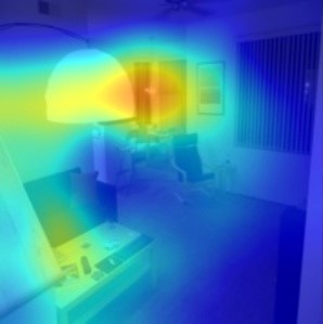
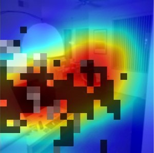
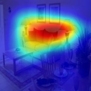
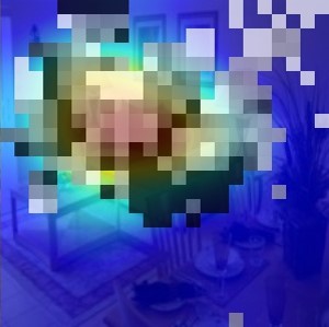
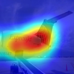
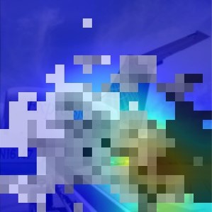
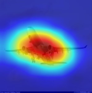
To peer into the impact of adversarial perturbations on individual images, we examine how the representation of concept detectors change while facing adversarial examples by attacking images from the same true class $t_{0}$ to the same target class $t$. Here the representation of a concept detector is visualized by the segmented input image determined by $\mathbf{M}_{k}(\mathbf{x})$. In Figure 10, we show two examples of attacks: ‘table lamp’-to-‘studio couch, day bed’ and ‘airliner’-to-‘seashore, seacoast’. We first note that most of low-level concepts (e.g., color and texture) are detected at shallow layers, consistent with Figure 9-b. In the attack ‘table lamp’-to-‘studio couch, day bed’, the color ‘orange’ detected at conv2_3 is less expressed for the adversarial image against the natural image. This aligns with human perception since ‘orange’ is related to ‘light’ and thus ‘table lamp’. By contrast, in the attack ‘airliner’-to-‘seashore, seacoast’, the color ‘blue’ is well detected at both natural and adversarial images, since ‘blue’ is associated with both ‘sky’ for ‘airliner’ and ‘sea’ for ‘seashore’. We also note that high-level concepts (e.g., part and object) dominate at deeper layers. At conv5_3, the expression of object concepts (e.g., lamp and airplane) relevant to the true label is suppressed. Meanwhile, the expression of object concepts (e.g., sofa and beach) relevant to the target label is promoted. This precisely reflects the activation promotion-suppression effect induced by adversarial perturbations. In Figure A8, we connect images in Figure 10 to PSR and CAM based visual explanation.

6 Insights of Interpretability for Improving Adversarial Robustness

First, PSE explains the effectiveness of detecting adversarial examples with feature attribution (?). It was shown in (?) that the input attribution scores of an adversarial example obtained by the leave-one-out method (?) yields a significantly larger variance than the case of natural image. The presence of a significant change on the probability of the top-$1$ class, when a pixel is removed from an adversarial example, is explainable. By PSE, the possible reason is that the seemingly random perturbation could play a critical role in promoting the confidence of the target label, e.g., Figure 7.

Second, hiding adversarial examples from CAM may be not easy. It was shown in (?) that adversarial examples can be crafted to fool CNNs, and at the same time keep their CAMs (w.r.t. the top-1 prediction class) intact. However, our results in Sec. 4 suggest that the discrepancy between CAMs of natural and adversarial examples exists w.r.t. both the true and the target label. Thus, we need to re-think whether or not it is easy to hide adversarial examples from network interpretation defined under the two-class or even all-class CAM distortion.

Third, network dissection implies the method of neuron masking to improve robustness. Since the sensitive units to adversarial perturbations exhibit strong interpretability, one could mitigate the effect of adversaries by masking these sensitive neurons with interpretation toward the target label. Our preliminary results in Table A2 of Appendix 4 show that the suggested neuron masking improves robustness at the cost of slight degradation on clean test accuracy.

7 Conclusions

In this work, we made a significant effort to understand the mechanism of adversarial attacks and provided its explanation at pixel, image and network levels. We showed that adversarial attacks play a significant role in activation promotion and suppression. The promotion-suppression effect is strongly associated with class-specific discriminative image regions. We also demonstrated that the interpretable adversarial pattern constrains the effectiveness of adversarial attacks. We further provided the first analysis of adversarial examples through network dissection, which builds the connection between the units’ sensitivity to imperceptible perturbations and their interpretability on semantic concepts. In the future, we would like to develop interpretability-driven defensive methods and consider the scenario of attack against interpretability, not just prediction.

Appendices of Interpreting Adversarial Examples by Activation Promotion and Suppression

1 Attack Generation

IFGSM attack (?; ?) produces adversarial examples by performing iterative fast gradient sign method (IFGSM), followed by an $\epsilon$-ball clipping. IFGSM attacks are designed to be fast, rather than optimal in terms of minimum perturbation.

C&W (?), EAD (?), and Str- attacks (?) can be unified in the following optimization framework,

$$\begin{array}[]{ll}\displaystyle\operatorname*{\text{minimize}}_{\bm{\delta}}&f(\mathbf{x}_{0}+\bm{\delta},t)+{\lambda}g(\bm{\delta})\\ \operatorname*{\text{subject to}}&(\mathbf{x}_{0}+\bm{\delta})\in[0,1]^{n},~{}h(\bm{\delta})\leq 0,\end{array}$$ (13)

where $f(\mathbf{x}_{0}+\bm{\delta},t)$ denotes a loss function for targeted misclassification, $g(\bm{\delta})$ is a regularization function that penalizes the norm of adversarial perturbations, $\lambda>0$ is a regularization parameter, and $h(\bm{\delta})$ places optionally hard constraints on $\bm{\delta}$. All C&W, EAD and Str- attacks enjoy a similar loss function

$$f(\mathbf{x}_{0}+\bm{\delta},t)=c\cdot\max\{ \max_{j\neq t}Z(\mathbf{x}_{0}+\bm{\delta})_{j}$$

$$-Z(\mathbf{x}_{0}+\bm{\delta})_{t},-\kappa\},$$ (14)

where $Z(\mathbf{x})_{j}$ is the $j$-th element of logits $Z(\mathbf{x})$, namely, the output before the last softmax layer in CNNs, and $\kappa$ is a confidence parameter. Clearly, as $\kappa$ increases, the minimization of $f$ would reach the target label with high confidence. In this paper, we set $\kappa=1$ by default. It is worth mentioning that problem (13) can be efficiently solved via alternating direction method of multipliers (ADMM) (?; ?), regardless of whether or not $g(\bm{\delta})$ is differentiable.

C&W attack (?) adopts the $\ell_{p}$ norm to penalize the strength of adversarial perturbations $\bm{\delta}$, namely, $g(\bm{\delta})=\|\bm{\delta}\|_{p}$ and $h(\bm{\delta})=0$ in (13), where $p\in\{0,2,\infty\}$. In practice, the squared $\ell_{2}$ norm is commonly used.

EAD attack (?) specifies the regularization term $\lambda g(\bm{\delta})$ as an elastic-net regularizer $\lambda_{1}\|\bm{\delta}\|_{2}^{2}+\lambda_{2}\|\bm{\delta}\|_{1}$ in (13), and $h(\bm{\delta})=0$. It has empirically shown that the use of elastic-net regularizer improves the transferability of adversarial examples.

Str-attack (?) takes into account the group-level sparsity of adversarial perturbations by choosing $g(\bm{\delta})$ as the group Lasso penalty (?). In the mean time, it constrains the pixel-level perturbation by setting $h(\bm{\delta})=\|\bm{\delta}\|_{\infty}-\epsilon$ for a tolerance $\epsilon>0$.

2 CAM-based Interpretation

Sensitivity of hyper-parameter $\nu$ to IS. Figure A1 presents IS against $\nu$ for IFGSM, C&W, EAD and Str attacks.

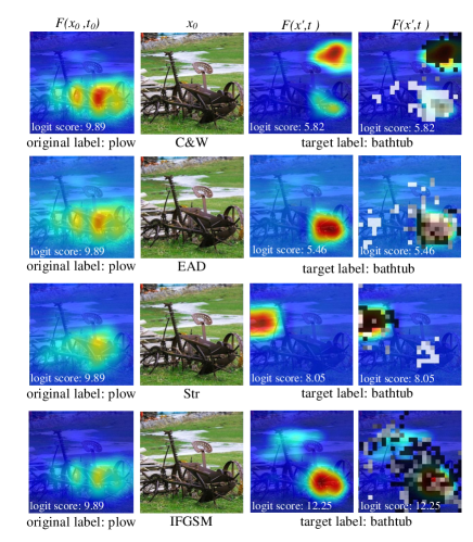
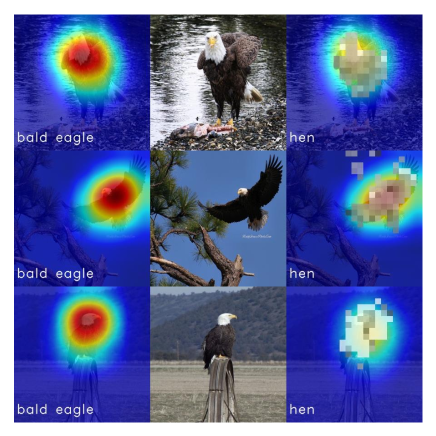
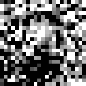
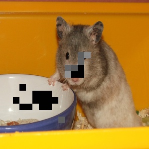
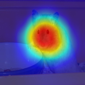
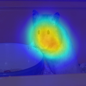
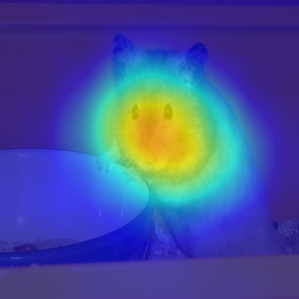
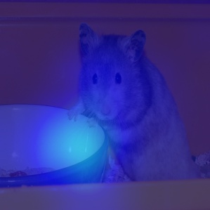
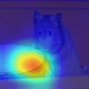
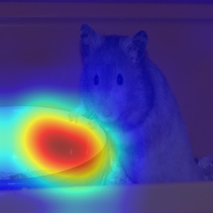
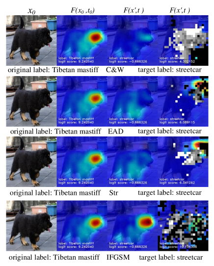
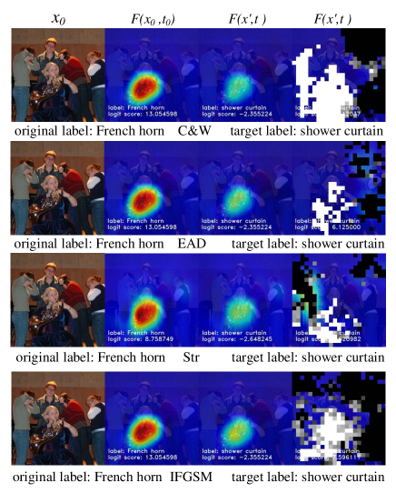
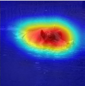
Additional results on CAM-based interpretation. In Figure A2, we demonstrate more examples of class-specific discriminative regions visualized by CAM, namely, $F(\mathbf{x}^{\prime},t_{0})$, $F(\mathbf{x}_{0},t_{0})$, $\mathbf{x}_{0}$, $F(\mathbf{x}_{0},t)$, $F(\mathbf{x}^{\prime},t)$. In Figure A3, we fix the orginal image together with its true and target labels to visualize the difference of attack methods through CAM. In Figure A4, we present the adversarial attack of multiple images with a fixed source-target label pair. As we can see, the balance-dominated perturbation pattern appears at the discriminative region of ‘eagle’. In Figure A5, we present the ‘hamster’-to-‘cup’ example, where objects of the original label and the target label exist simultaneously. We observe that the adversary shows suppression on the discriminative region of the original label and promotion on the discriminative region of the target label. Compared to the C&W attack, Str-attack is more effective in both suppressing and promotion since it perturbs less pixels. In Figure A6, images involve more heterogeneous and complex backgrounds. As we can see, an effective adversarial attack (e.g., Str-attack) perturbs less but more meaningful pixels, which have a better correspondence with the discriminative image regions of the original and target classes. In Figure A7, we present a ‘hippocampus’-to-‘streetcar’ example with refined attacks under $\mathcal{S}_{1}$. As we can see, it is possible to obtain a more effective attack by perturbing less but ‘right’ pixels (i.e., with better correspondence with discriminative image regions).

3 Effectiveness of Refined Adversarial Pattern

We consider the following unified optimization problem to refine adversarial attacks

$$\begin{array}[]{ll}\displaystyle\operatorname*{\text{minimize}}_{\bm{\delta}}&f(\mathbf{x}_{0}+\bm{\delta},t)+\lambda g(\bm{\delta})\\ \operatorname*{\text{subject to}}&(\mathbf{x}_{0}+\bm{\delta})\in[0,1]^{n},~{}h(\bm{\delta})\leq 0\\ &\delta_{i}=0,~{}\text{if}~{}i\notin\mathcal{S}_{k},~{}\text{$k=1$ or $2$},\end{array}$$ (18)

where we represent the refinement operations (a) and (b) through the constraint sets $\mathcal{S}_{1}=\{\forall i\,|\,s_{i}>\beta\}$ for a positive threshold $\beta$ and $\mathcal{S}_{2}=\{\forall i\,|\,[B(\mathbf{x}_{0},t_{0})]_{i}>0\}$. In $\mathcal{S}_{1}$, $s_{i}$ defined by (3) characterizes the strength of the adversarial pattern. In $\mathcal{S}_{2}$, $B(\mathbf{x}_{0},t_{0})$ defined by (7) localizes pixels corresponding to the most discriminative region associated with the true label. Problem (18) can similarly be solved as (13), with an additional projection on the sparse constraints given by $\mathcal{S}_{1}$ and $\mathcal{S}_{2}$.

We present the effectiveness of attacks with refinement under $\mathcal{S}_{1}$ in Table A1. Here the effectiveness of an attack is characterized by its attack success rate (ASR) as well as $\ell_{p}$-norm distortions. We find that many pixel-level adversarial perturbations are redundant, in terms of the reduction in the $\ell_{0}$ norm of $\bm{\delta}$, which can be removed without losing effectiveness in the attack success rate and $\ell_{p}$-norm distortions for $p>0$.

4 Interpretation via Network Dissection

In Figure A8, we connect images in Figure 10 to PSR and CAM based visual explanation. For example, the suppressed image region identified by PSR (white color) corresponds to the interpretable activation of object concept airplane in Figure 10. And the promoted image region identified by PSR (black color) corresponds to the interpretable activation of scene concept beach.

In Table A2, we report the clean test accuracy (CTA) and the adversarial test accuracy (ATA) under three masking settings on the last convolutional layer of $\mathrm{conv}5$: a) our proposed masking over top $10$ sensitive units with concept-level interpretability, b) random masking over $10$ units, and c) no masking. ATA is obtained by perturbing $1000$ randomly selected test images using $k$-step PGD attack (?), where $k\in\{10,20,50,100\}$. Our preliminary results show that the proposed approach yields the highest ATA, balanced with slight degradation on CTA.

Figure A1: IS versus $\nu$ for $4$ attack types.

Figure A2: CAMs of two natural/adversarial examples (in rows), generated by C&W attack, where $F(\mathbf{x}^{\prime},t_{0})$, $F(\mathbf{x}_{0},t_{0})$, $\mathbf{x}_{0}$, $F(\mathbf{x}_{0},t)$, $F(\mathbf{x}^{\prime},t)$ are shown from the left to the right at each row.

Figure A3: Four adversarial examples with CAM visualization generated by C&W, EAD, Str, and IFGSM attacks, respectively. Left to right: $F(\mathbf{x}_{0},t_{0})$, $x_{0}$, $F(\mathbf{x}^{\prime},t)$, and overlaid PSR $r_{i}$ on $F(\mathbf{x}^{\prime},t)$ at locations of the top $70\%$ most significant perturbed grids ranked by $s_{i}$. Here CAMs at each row are normalized with respect to their maximum value.

Figure A4: Multiple images with a fixed source-target label pair: CAM with respect to the source label ‘bald eagle’ (1 column), original image ‘bald eagle’ (2 column), CAM with respect to target label ‘hen’ together with C&W perturbation patterns (3 column), which is measured by promotion-suppression ratio (PSR), i.e. suppression- (white), promotion- (black), and balance-dominated adversaries (gray).

	original		C&W attack	Str-attack
		PSR over perturbed grids
CAM w.r.t. $t_{0}$
CAM w.r.t. $t$

Figure A5: Visual explanation of the ‘hamster’-to-‘cup’ example crafted by C&W and Str-attack, where the true label $t_{0}$ is ‘hamster’, and the target label $t$ is ‘cup’. The first row is the natural image and PSRs over perturbed grids. The second (third) row is CAM with respect to the column-wise natural/adversarial example and the row-wise label.

Figure A6: Attacking images with complex background under C&W, EAD, Str-, and IFGSM attacks.

original		C&W	EAD	Str	IFGSM
	w/o refine
	with refine

Figure A7: The ‘hippopotamus’-to-‘streetcar’ adversarial example with and without refinement under $\mathcal{S}_{1}$. Here the left-bottom subplot shows CAM of the original image w.r.t. the true label ‘hippopotamus’, and the right subplots present PSRs of unrefined and refined grid-level perturbations overlaid on CAMs of adversarial examples w.r.t. the target label ‘streetcar’.

adv. examples	$F(\bm{x}_{0},t_{0})$	$F(\bm{x}^{\prime},t)$ & PSRs
$t_{0}$: table lamp – $t$: studio coach
$t_{0}$: airliner – $t$: seashore

Figure A8: Interpreting adversarial perturbations via CAM and PSR. Image examples are from Figure  10. For PSR, only the top $70\%$ most significant perturbed grids ranked by $\{s_{i}\}$ (3) are shown. The white and black colors represent the suppression-dominated regions ($r_{i}<-1$) and the promotion-dominated regions ($r_{i}>1$), respectively. The gray color corresponds to balance-dominated perturbations ($r_{i}\in[-1,1]$).

Table A1: Attack performance of adversarial perturbations with and without refinement under $\mathcal{S}_{1}$ over $5000$ images.

attack model $\ell_{0}$ $\ell_{1}$ $\ell_{2}$ $\ell_{\infty}$ ASR original ($\bm{\delta}$) refine (${\bm{\delta}}_{\mathcal{S}}$) original refine original refine original refine refine IFGSM Resnet 266031 61055 1122.56 176.08 2.625 1.87 0.017 0.035 96.7% Incep. 266026 59881 812.94 155.89 1.926 1.22 0.019 0.033 100% C&W Resnet 268117 21103 183.65 134.26 0.697 0.727 0.028 0.029 100% Incep. 268123 22495 144.94 96.75 0.650 0.673 0.028 0.034 100% EAD Resnet 66584 20147 42.57 63.28 1.520 1.233 0.234 0.096 100% Incep. 69677 18855 30.17 45.88 1.289 1.107 0.229 0.083 100% Str Resnet 30823 18744 119.76 110.54 1.250 1.132 0.105 0.087 100% Incep. 27873 15967 86.55 82.33 1.174 0.985 0.103 0.072 100%

Table A2: Evaluation of neuron masking on clean test accuracy (CTA) and adversarial test accuracy (ATA) against $k$-step PGD attacks.

CTA ATA ($10$-PGD) ATA ($20$-PGD) ATA ($50$-PGD) ATA ($100$-PGD) ours 75.9% 60.1% 51.5% 39.7% 33.6% random masking 77.0% 40.5% 28.7% 18.3% 14.3% no masking 78.2% 41.7% 31.0% 18.8% 15.7%

References

- [Athalye, Carlini, and Wagner 2018] Athalye, A.; Carlini, N.; and Wagner, D. 2018. Obfuscated gradients give a false sense of security: Circumventing defenses to adversarial examples. arXiv preprint arXiv:1802.00420.
- [Bau et al. 2017] Bau, D.; Zhou, B.; Khosla, A.; Oliva, A.; and Torralba, A. 2017. Network dissection: Quantifying interpretability of deep visual representations. arXiv preprint arXiv:1704.05796.
- [Bau et al. 2019] Bau, D.; Zhu, J.-Y.; Strobelt, H.; Zhou, B.; Tenenbaum, J. B.; Freeman, W. T.; and Torralba, A. 2019. Visualizing and understanding generative adversarial networks. In International Conference on Learning Representations.
- [Boyd et al. 2011] Boyd, S.; Parikh, N.; Chu, E.; Peleato, B.; Eckstein, J.; et al. 2011. Distributed optimization and statistical learning via the alternating direction method of multipliers. Foundations and Trends® in Machine Learning 3(1):1–122.
- [Brown et al. 2017] Brown, T. B.; Mané, D.; Roy, A.; Abadi, M.; and Gilmer, J. 2017. Adversarial patch. arXiv preprint arXiv:1712.09665.
- [Carlini and Wagner 2017a] Carlini, N., and Wagner, D. 2017a. Adversarial examples are not easily detected: Bypassing ten detection methods. In Proceedings of the 10th ACM Workshop on Artificial Intelligence and Security, 3–14. ACM.
- [Carlini and Wagner 2017b] Carlini, N., and Wagner, D. 2017b. Towards evaluating the robustness of neural networks. In Security and Privacy (SP), 2017 IEEE Symposium on, 39–57. IEEE.
- [Carlini et al. 2016] Carlini, N.; Mishra, P.; Vaidya, T.; Zhang, Y.; Sherr, M.; Shields, C.; Wagner, D.; and Zhou, W. 2016. Hidden voice commands. In USENIX Security Symposium, 513–530.
- [Carter et al. 2019] Carter, S.; Armstrong, Z.; Schubert, L.; Johnson, I.; and Olah, C. 2019. Activation atlas. Distill. https://distill.pub/2019/activation-atlas.
- [Chattopadhay et al. 2018] Chattopadhay, A.; Sarkar, A.; Howlader, P.; and Balasubramanian, V. N. 2018. Grad-cam++: Generalized gradient-based visual explanations for deep convolutional networks. In 2018 IEEE Winter Conference on Applications of Computer Vision (WACV), 839–847. IEEE.
- [Chen et al. 2017] Chen, P.-Y.; Sharma, Y.; Zhang, H.; Yi, J.; and Hsieh, C.-J. 2017. Ead: elastic-net attacks to deep neural networks via adversarial examples. arXiv preprint arXiv:1709.04114.
- [Dong et al. 2017] Dong, Y.; Su, H.; Zhu, J.; and Bao, F. 2017. Towards interpretable deep neural networks by leveraging adversarial examples. arXiv preprint arXiv:1708.05493.
- [Finlay, Oberman, and Abbasi 2018] Finlay, C.; Oberman, A.; and Abbasi, B. 2018. Improved robustness to adversarial examples using lipschitz regularization of the loss. arXiv preprint arXiv:1810.00953.
- [Goodfellow, Shlens, and Szegedy 2015] Goodfellow, I.; Shlens, J.; and Szegedy, C. 2015. Explaining and harnessing adversarial examples. 2015 ICLR arXiv preprint arXiv:1412.6572.
- [He et al. 2016] He, K.; Zhang, X.; Ren, S.; and Sun, J. 2016. Deep residual learning for image recognition. In Proceedings of the IEEE conference on computer vision and pattern recognition, 770–778.
- [Karmon, Zoran, and Goldberg 2018] Karmon, D.; Zoran, D.; and Goldberg, Y. 2018. Lavan: Localized and visible adversarial noise. arXiv preprint arXiv:1801.02608.
- [Kurakin, Goodfellow, and Bengio 2016] Kurakin, A.; Goodfellow, I.; and Bengio, S. 2016. Adversarial examples in the physical world. arXiv preprint arXiv:1607.02533.
- [Kurakin, Goodfellow, and Bengio 2017] Kurakin, A.; Goodfellow, I. J.; and Bengio, S. 2017. Adversarial machine learning at scale. 2017 ICLR arXiv preprint arXiv:1611.01236.
- [Luo et al. 2018] Luo, T.; Cai, T.; Zhang, M.; Chen, S.; and Wang, L. 2018. Random mask: Towards robust convolutional neural networks.
- [Madry et al. 2017] Madry, A.; Makelov, A.; Schmidt, L.; Tsipras, D.; and Vladu, A. 2017. Towards deep learning models resistant to adversarial attacks. arXiv preprint arXiv:1706.06083.
- [Papernot et al. 2016a] Papernot, N.; McDaniel, P.; Jha, S.; Fredrikson, M.; Celik, Z. B.; and Swami, A. 2016a. The limitations of deep learning in adversarial settings. In Security and Privacy (EuroS&P), 2016 IEEE European Symposium on, 372–387. IEEE.
- [Papernot et al. 2016b] Papernot, N.; McDaniel, P.; Wu, X.; Jha, S.; and Swami, A. 2016b. Distillation as a defense to adversarial perturbations against deep neural networks. In Security and Privacy (SP), 2016 IEEE Symposium on, 582–597. IEEE.
- [Petsiuk, Das, and Saenko 2018] Petsiuk, V.; Das, A.; and Saenko, K. 2018. Rise: Randomized input sampling for explanation of black-box models. arXiv preprint arXiv:1806.07421.
- [Selvaraju et al. 2017] Selvaraju, R. R.; Cogswell, M.; Das, A.; Vedantam, R.; Parikh, D.; and Batra, D. 2017. Grad-cam: Visual explanations from deep networks via gradient-based localization. In Proceedings of the IEEE International Conference on Computer Vision, 618–626.
- [Sinha, Namkoong, and Duchi 2018] Sinha, A.; Namkoong, H.; and Duchi, J. 2018. Certifying some distributional robustness with principled adversarial training.
- [Szegedy et al. 2016] Szegedy, C.; Vanhoucke, V.; Ioffe, S.; Shlens, J.; and Wojna, Z. 2016. Rethinking the inception architecture for computer vision. 2016 IEEE Conference on Computer Vision and Pattern Recognition (CVPR) 2818–2826.
- [Xiao et al. 2018] Xiao, C.; Zhu, J.-Y.; Li, B.; He, W.; Liu, M.; and Song, D. 2018. Spatially transformed adversarial examples. In International Conference on Learning Representations.
- [Xu et al. 2019a] Xu, K.; Chen, H.; Liu, S.; Chen, P.-Y.; Weng, T.-W.; Hong, M.; and Lin, X. 2019a. Topology attack and defense for graph neural networks: An optimization perspective. In International Joint Conference on Artificial Intelligence (IJCAI).
- [Xu et al. 2019b] Xu, K.; Liu, S.; Zhao, P.; Chen, P.-Y.; Zhang, H.; Fan, Q.; Erdogmus, D.; Wang, Y.; and Lin, X. 2019b. Structured adversarial attack: Towards general implementation and better interpretability. In International Conference on Learning Representations.
- [Yang et al. 2019] Yang, P.; Chen, J.; Hsieh, C.-J.; Wang, J.-L.; and Jordan, M. I. 2019. Ml-loo: Detecting adversarial examples with feature attribution. arXiv preprint arXiv:1906.03499.
- [Ye et al. 2019] Ye, S.; Xu, K.; Liu, S.; Cheng, H.; Lambrechts, J.-H.; Zhang, H.; Zhou, A.; Ma, K.; Wang, Y.; and Lin, X. 2019. Adversarial robustness vs model compression, or both? International Conference on Computer Vision (ICCV-2019).
- [Yu, Dong, and Chen 2018] Yu, F.; Dong, Q.; and Chen, X. 2018. Asp: A fast adversarial attack example generation framework based on adversarial saliency prediction. arXiv preprint arXiv:1802.05763.
- [Yuan and Lin 2006] Yuan, M., and Lin, Y. 2006. Model selection and estimation in regression with grouped variables. Journal of the Royal Statistical Society: Series B (Statistical Methodology) 68(1):49–67.
- [Zeiler and Fergus 2014] Zeiler, M. D., and Fergus, R. 2014. Visualizing and understanding convolutional networks. In European conference on computer vision, 818–833. Springer.
- [Zhang et al. 2018] Zhang, X.; Wang, N.; Ji, S.; Shen, H.; and Wang, T. 2018. Interpretable deep learning under fire. arXiv preprint arXiv:1812.00891.
- [Zhou et al. 2016] Zhou, B.; Khosla, A.; Lapedriza, A.; Oliva, A.; and Torralba, A. 2016. Learning deep features for discriminative localization. In Proceedings of the IEEE Conference on Computer Vision and Pattern Recognition, 2921–2929.