Loop Homology of Bi-secondary Structures

Andrei C. Bura anbur12@vt.edu Qijun He qhe196@gmail.com Christian M. Reidys duck@santafe.edu Department of Mathematics, Virginia Tech, 225 Stanger Street, Blacksburg, VA 24061-1026 Biocomplexity Institute of Virginia Tech, 1015 Life Sciences Circle Blacksburg, VA 24061 Biocomplexity Institute and Initiative, University of Virginia, 995 Research Park Boulevard, Charlottesville, VA 22911 Department of Mathematics, University of Virginia, 141 Cabell Dr, Charlottesville, VA 22903
Abstract

In this paper we compute the loop homology of bi-secondary structures. Bi-secondary structures were introduced by Haslinger and Stadler and are pairs of RNA secondary structures, i.e. diagrams having non-crossing arcs in the upper half-plane. A bi-secondary structure is represented by drawing its respective secondary structures in the upper and lower half-plane. An RNA secondary structure has a loop decomposition, where a loop corresponds to a boundary component, regarding the secondary structure as an orientable fatgraph. The loop-decomposition of secondary structures facilitates the computation of its free energy and any two loops intersect either trivially or in exactly two vertices. In bi-secondary structures the intersection of loops is more complex and is of importance in current algorithmic work in bio-informatics and evolutionary optimization. We shall construct a simplicial complex capturing the intersections of loops and compute its homology. We prove that only the zeroth and second homology groups are nontrivial and furthermore show that the second homology group is free. Finally, we provide evidence that the generators of the second homology group have a bio-physical interpretation: they correspond to pairs of mutually exclusive substructures.

keywords:
RNA, bi-secondary structure, loop, nerve, simplicial homology.
journal: Discrete Mathematics

1 Introduction

RNA sequences are single stranded nucleic acids that, in difference to DNA, can form a plethora of structural conformations. Over the last several decades, researchers have discovered an increasing number of important roles for RNA [1]. The folded structure of RNA is critically important to its function [2] and has been extensively studied at the coarse grained level of base pairing interactions. This leads to the notion of RNA secondary structures [3], that represent particular contact matrices and do not take into account the embedding in 333-space [4].

The thermodynamic stability of a secondary structure is characterized by its free energy, and is computed by summing the energy contribution of its loops [5, 6]. Prediction of the minimum free energy (i.e. the most stable) secondary structure for a given sequence, is an important problem at the most basic biological level [7].

The first mfe-folding algorithms for RNA secondary structures are due to [8, 4, 9]. Waterman studied the loop decomposition and the recursive construction of secondary structures and derived the first dynamic programming (DP) folding routines for secondary structures [10]. The DP routine facilitates polynomial time folding algorithms [11, 12, 13] and partition function calculation [14]. In [15], Haslinger and Stadler extended the notion of secondary structures to bi-secondary structures in order to study pseudoknotted structures, RNA structures exhibiting cross serial interactions [16]. Bi-secondary structures play furthermore a central role for studying sequences that can realize two, oftentimes mutually exclusive, conformations, in the context of evolutionary transitions [17] and in the study of RNA riboswitches, i.e. sequences that exhibit two stable configurations [18].

The partition function of structures w.r.t. a fixed sequence has a dual: the partition function of sequences compatible with a fixed structure [19]. Partition function and Boltzmann sampling have a variety of applications in sequence design [20, 21], extracting structural semantics [22] and to analyze mutational robustness [23].

RNA structures, viewed as abstract diagrams or trees, have been studied in enumerative combinatorics [10, 24, 25, 15], algebraic combinatorics [26], matrix-models [27, 28] and topology [29, 30, 31].

In [24], a bijection between linear trees and secondary structures was constructed. This facilitated beautiful, explicit formulae for the number of secondary structures on n𝑛n vertices, having exactly k𝑘k arcs.
Jin et al. [26] enumerate k𝑘k-non-crossing RNA structures, based on the bijection given by Chen et al. [32], between k𝑘k-non-crossing partial matchings and walks in k1superscript𝑘1\mathbb{Z}^{k-1} which remain in the interior of the Weyl-chamber C0subscript𝐶0C_{0}. The bijection between oscillating tableaux and matchings originated from Stanley [33] and was generalized by Sundaram [34].
Penner and Waterman connected RNA structures with topology by studying the space of RNA secondary structures. They proved that the geometrical realizations of the associated complex of secondary structures is a sphere [35]. In [29], Bon et al. presented a topological classification of secondary structures, based on matrix models.
In the course of computing the Euler characteristics of the Moduli space of a curve, [36], Harer and Zagier computed the generating function of the number of linear chord diagrams of genus g𝑔g with n𝑛n chords. Based on this line of work, Andersen et al. [28], enumerated the number of chord diagrams of fixed genus with specified numbers of backbones and chords. Such an enumeration of chord diagrams provides the number of secondary structures of a given genus as well as the number of cells in Riemann’s moduli spaces for bordered surfaces. This was done by using Hermitian matrix model techniques and topological recursions along the lines of [37]. Employing an augmented version of the topological recursion on unicellular maps of Chapuy [38], Huang et al [31] derived explicit expressions for the coefficients of the generating polynomial of topological shapes of RNA structures and the generating function of RNA structures of genus g𝑔g. This lead to uniform sampling algorithms for structures of fixed topological genus as well as a natural way to resolve crossings in pseudoknotted structures [39].

Bi-secondary structures emerge naturally in the context of evolutionary transitions, since they are closely connected to sets of sequences, that are simultaneously compatible with two structures [40]. This paper is motivated by the dynamical programming (DP) routine of Huang [41], that is based on sub-problems associated with sets of loops. The sub-problems were constructed incrementally by adding one loop at a time, where subsequently added nucleotides affect the energy calculation if they appear in multiple loops. This naturally leads one to consider intersections of loops and eventually to introduce the nerve of loops as a simplicial complex.

In this paper, we study the homology of bi-secondary structures [15]. We show that for any bi-secondary structure R𝑅R, we have only two nontrivial homology groups, H0(R)subscript𝐻0𝑅H_{0}(R) and H2(R)subscript𝐻2𝑅H_{2}(R). The key to establish H1(R)=0subscript𝐻1𝑅0H_{1}(R)=0 is to establish in Lemma 6 the existence of certain, spanning, sub 111-skeleta, whose existence follows from an inductive argument over the arcs of one of the secondary structures. These skeleta give rise to specific trees, which in turn allow one to systematically process elements of Ker(1)Kersubscript1\text{\rm Ker}(\partial_{1}). We show that H0(R)subscript𝐻0𝑅H_{0}(R)\cong\mathbb{Z} and H2(R)k=1rsubscript𝐻2𝑅superscriptsubscriptdirect-sum𝑘1𝑟H_{2}(R)\cong\bigoplus_{k=1}^{r}\mathbb{Z}, introducing the rank of H2(R)subscript𝐻2𝑅H_{2}(R) as a new invariant of the bi-secondary structures. We show that H2(R)subscript𝐻2𝑅H_{2}(R) is free by showing that it is a subgroup of a free group, whose freeness in turn is a consequence of Lemma 4 which guarantees the existence of exposed faces of 333-simplices. We then discuss the new invariant, observing that all RNA riboswitch sequences in data-bases exhibit rank(H2(R))=1ranksubscript𝐻2𝑅1\text{\rm rank}(H_{2}(R))=1, seldomly assumed by random secondary structure pairs and provide an outlook on future work.

2 Some basic facts

We shall begin by defining loops in an RNA secondary structure and then present results on its loop decomposition.

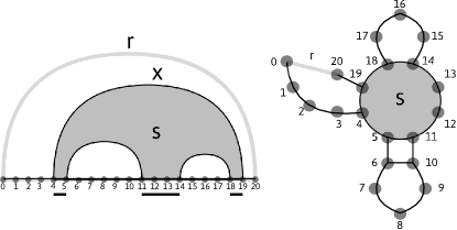
An RNA diagram S𝑆S over [n]delimited-[]𝑛[n], is a vertex-labeled graph whose vertices are drawn on the horizontal axis and labeled by [n]={1,,n}delimited-[]𝑛1𝑛[n]=\{1,\ldots,n\}. An arc (i,j)𝑖𝑗(i,j), is an ordered pair of vertices, which represents the base pairing between the i𝑖i-th and j𝑗j-th nucleotides in the RNA structure. Furthermore, each vertex can be paired with at most one other vertex, and the arc that connects them is drawn in the upper half-plane. We introduce two “formal” vertices associated with positions 00 and n+1𝑛1n+1, respectively, closing any diagram by the arc (0,n+1)0𝑛1(0,n+1), called the rainbow. The set [0,n+1]0𝑛1[0,n+1] is called the diagram’s backbone, see Figure 1.

Let S𝑆S be an RNA diagram over [n]delimited-[]𝑛[n]. Two arcs (i,j)𝑖𝑗(i,j) and (p,q)𝑝𝑞(p,q) are called crossing if and only if i<p<j<q𝑖𝑝𝑗𝑞i<p<j<q. S𝑆S is called a secondary structure if it does not contain any crossing arcs. The arcs of S𝑆S can be endowed with a partial order as follows: (k,l)S(i,j)i<k<l<jiffsubscriptprecedes𝑆𝑘𝑙𝑖𝑗𝑖𝑘𝑙𝑗(k,l)\prec_{S}(i,j)\iff i<k<l<j. We denote this by (S,S)𝑆subscriptprecedes𝑆(S,\prec_{S}) and call it the arc poset of S𝑆S. Finally, an interval [i,j]𝑖𝑗[i,j] on the backbone is the set of vertices {i,i+1,,j1,j}𝑖𝑖1𝑗1𝑗\{i,i+1,\ldots,j-1,j\}.

Let S𝑆S be a secondary structure over [n]delimited-[]𝑛[n]. A loop s𝑠s in S𝑆S is a subset of vertices, represented as a disjoint union of a sequence of contiguous blocks on the backbone of S𝑆S, s=˙i=1k[ai,bi]𝑠superscriptsubscript˙𝑖1𝑘subscript𝑎𝑖subscript𝑏𝑖s=\dot{\bigcup}_{i=1}^{k}[a_{i},b_{i}], such that (a1,bk)subscript𝑎1subscript𝑏𝑘(a_{1},b_{k}) and (bi,ai+1)subscript𝑏𝑖subscript𝑎𝑖1(b_{i},a_{i+1}), for 1ik11𝑖𝑘11\leq i\leq k-1, are arcs and such that any other interval-vertices are unpaired. Let αssubscript𝛼𝑠\alpha_{s} denote the unique, maximal arc (a1,bk)subscript𝑎1subscript𝑏𝑘(a_{1},b_{k}) of the loop.

In this paper we shall identify a secondary structure with its set of loops. Let S𝑆S be a secondary structure over [n]delimited-[]𝑛[n] and s=˙i=1k[ai,bi]𝑠superscriptsubscript˙𝑖1𝑘subscript𝑎𝑖subscript𝑏𝑖s=\dot{\bigcup}_{i=1}^{k}[a_{i},b_{i}] a loop in S𝑆S, then
(1)1(1) each unpaired vertex is contained in exactly one loop,
(2)2(2) (a1,bk)subscript𝑎1subscript𝑏𝑘(a_{1},b_{k}) is maximal w.r.t. Ssubscriptprecedes𝑆\prec_{S} among all arcs contained in s𝑠s, i.e. there is a bijection between arcs and loops, mapping each loop to its maximal arc,
(3)3(3) the Hasse diagram of the S𝑆S arc-poset is a rooted tree Tr(S)Tr𝑆\text{Tr}(S), having the rainbow arc as root,
(4)4(4) each non-rainbow arc appears in exactly two loops.
Refer to caption
Figure 1: LHS: a secondary structure, S𝑆S, and a distinguished loop s=[4,5][11,14][18,19]𝑠4511141819s=[4,5]\cup[11,14]\cup[18,19]. r𝑟r is the rainbow arc and αs=xsubscript𝛼𝑠𝑥\alpha_{s}=x. RHS: S𝑆S represented as a planar RNA𝑅𝑁𝐴RNA molecule.
Proposition 1.

Let s𝑠s, ssuperscript𝑠s^{\prime} and s′′superscript𝑠′′s^{\prime\prime} be three distinct loops in a secondary structure S𝑆S. Then
(1) sss′′=𝑠superscript𝑠superscript𝑠′′s\cap s^{\prime}\cap s^{\prime\prime}=\varnothing, (2) ss𝑠superscript𝑠s\cap s^{\prime}\neq\varnothing implies |ss|=2𝑠superscript𝑠2|s\cap s^{\prime}|=2.

Proof.

Vertices of S𝑆S are either paired or unpaired. In the latter case, they are contained in exactly one loop. In the former, by construction, they are endpoints of arcs and contained in exactly two distinct loops. Hence, no vertex can be contained in three distinct loops. In case of ss𝑠superscript𝑠s\cap s^{\prime}\neq\varnothing the loops intersect in the endpoints of exactly one arc, which is maximal for exactly of of them, whence |ss|=2𝑠superscript𝑠2|s\cap s^{\prime}|=2. ∎

In this section we introduce bi-secondary structures and their nerves. To this end we introduce the nerve over a finite collection of sets:

Let X={x0,x1,,xm}𝑋subscript𝑥0subscript𝑥1subscript𝑥𝑚X=\{x_{0},x_{1},\ldots,x_{m}\} be a collection of finite sets. We call Y={xi0,,xid}X𝑌subscript𝑥subscript𝑖0subscript𝑥subscript𝑖𝑑𝑋Y=\{x_{i_{0}},\ldots,x_{i_{d}}\}\subseteq X a d𝑑d-simplex of X𝑋X iff k=0dxiksuperscriptsubscript𝑘0𝑑subscript𝑥subscript𝑖𝑘\bigcap_{k=0}^{d}x_{i_{k}}\neq\varnothing. We set Ω(Y)=k=0dxikΩ𝑌superscriptsubscript𝑘0𝑑subscript𝑥subscript𝑖𝑘\Omega(Y)=\bigcap_{k=0}^{d}x_{i_{k}} and refer to ω(Y)=|Ω(Y)|0𝜔𝑌Ω𝑌0\omega(Y)=|\Omega(Y)|\neq 0 as the weight of Y𝑌Y. Let Kd(X)subscript𝐾𝑑𝑋K_{d}(X) be the set of all d𝑑d-simplices of X𝑋X, then the nerve of X𝑋X is

K(X)=˙d=0Kd(X)2X.𝐾𝑋superscriptsubscript˙𝑑0subscript𝐾𝑑𝑋superscript2𝑋K(X)=\dot{\bigcup}_{d=0}^{\infty}K_{d}(X)\subseteq 2^{X}.

A dsuperscript𝑑d^{\prime}-simplex YK(X)superscript𝑌𝐾𝑋Y^{\prime}\in K(X) is called a dsuperscript𝑑d^{\prime}-face of Y𝑌Y if d<dsuperscript𝑑𝑑d^{\prime}<d and YYsuperscript𝑌𝑌Y^{\prime}\subseteq Y. By construction, K(X)𝐾𝑋K(X) is an abstract simplicial complex. Let S𝑆S be a secondary structure over [n]delimited-[]𝑛[n]. The geometric realization of K(S)𝐾𝑆K(S), the nerve over the set of loops of S𝑆S, is a tree. By means of the correspondence between arcs and loops, this tree of loops is isomorphic to Tr(S)Tr𝑆\text{Tr}(S).

Definition 1.

Given two secondary structures S𝑆S and T𝑇T over [n]delimited-[]𝑛[n], we refer to the pair R=(S,T)𝑅𝑆𝑇R=(S,T) as a bi-secondary structure. Let ST𝑆𝑇S\cup T be the loop set of R𝑅R and K(R)=˙d=0Kd(R)𝐾𝑅superscriptsubscript˙𝑑0subscript𝐾𝑑𝑅K(R)=\dot{\bigcup}_{d=0}^{\infty}K_{d}(R) its nerve of loops.

We represent the diagram of a bi-secondary structure R=(S,T)𝑅𝑆𝑇R=(S,T) with the arcs of S𝑆S in the upper half plane while the arcs of T𝑇T reside in the lower half plane. Let R=(S,T)𝑅𝑆𝑇R=(S,T) be a bi-secondary structure with loop nerve K(R)𝐾𝑅K(R). A 111-simplex Y={ri0,ri1}K1(R)𝑌subscript𝑟subscript𝑖0subscript𝑟subscript𝑖1subscript𝐾1𝑅Y=\{r_{i_{0}},r_{i_{1}}\}\in K_{1}(R) is called pure if ri0subscript𝑟subscript𝑖0r_{i_{0}} and ri1subscript𝑟subscript𝑖1r_{i_{1}} are loops in the same secondary structure and mixed, otherwise.
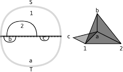
Suppose Y𝑌Y is a pure 111-simplex in K(R)𝐾𝑅K(R), then by Proposition 1 we have ω(Y)=2𝜔𝑌2\omega(Y)=2, see Figure 2.

Refer to caption
Figure 2: LHS: a bi-secondary structure R=(S,T)𝑅𝑆𝑇R=(S,T). RHS: the geometric realization of its loop nerve, K(R)𝐾𝑅K(R). the 111-simplices {c,1}𝑐1\{c,1\} and {1,2}12\{1,2\} are mixed and pure, respectively.
Lemma 1.

Let R=(S,T)𝑅𝑆𝑇R=(S,T) be a bi-secondary structure with nerve K(R)𝐾𝑅K(R). For any YK2(R)𝑌subscript𝐾2𝑅Y\in K_{2}(R), exactly one of its three 111-faces is pure, the other two being mixed. Furthermore, we have ω(Y)2𝜔𝑌2\omega(Y)\leq 2.

Proof.

Let Y={r0,r1,r2}K2(R)𝑌subscriptsuperscript𝑟0subscriptsuperscript𝑟1subscriptsuperscript𝑟2subscript𝐾2𝑅Y=\{r^{\prime}_{0},r^{\prime}_{1},r^{\prime}_{2}\}\in K_{2}(R) be a 222-simplex of K(R)𝐾𝑅K(R). By Proposition 1, i=0,1,2risubscript𝑖012subscriptsuperscript𝑟𝑖\cap_{i=0,1,2}r^{\prime}_{i}\neq\varnothing implies that not all three loops can be from the same structure. W.l.o.g. suppose r0,r1Ssubscriptsuperscript𝑟0subscriptsuperscript𝑟1𝑆r^{\prime}_{0},r^{\prime}_{1}\in S and r2Tsubscriptsuperscript𝑟2𝑇r^{\prime}_{2}\in T. Certainly Z={r0,r1}𝑍subscriptsuperscript𝑟0subscriptsuperscript𝑟1Z=\{r^{\prime}_{0},r^{\prime}_{1}\} is a pure 111-face of Y𝑌Y and two other 111-faces of Y𝑌Y are by construction mixed since they contain r3Tsubscriptsuperscript𝑟3𝑇r^{\prime}_{3}\in T. For any 111-face Zsuperscript𝑍Z^{\prime} of Y𝑌Y, we have ω(Y)ω(Z)𝜔𝑌𝜔superscript𝑍\omega(Y)\leq\omega(Z^{\prime}) and Proposition 1 guarantees ω(Z)=2𝜔𝑍2\omega(Z)=2, whence the lemma. ∎

Lemma 2.

Let R=(S,T)𝑅𝑆𝑇R=(S,T) be a bi-secondary structure with nerve K(R)𝐾𝑅K(R) and let Y={r0,r1,r2,r3}K3(R)𝑌subscript𝑟0subscript𝑟1subscript𝑟2subscript𝑟3subscript𝐾3𝑅Y=\{r_{0},r_{1},r_{2},r_{3}\}\in K_{3}(R) be a 333-simplex. Then we have
(a) Y={s0,s1,t0,t1}𝑌subscript𝑠0subscript𝑠1subscript𝑡0subscript𝑡1Y=\{s_{0},s_{1},t_{0},t_{1}\}, where s0,s1Ssubscript𝑠0subscript𝑠1𝑆s_{0},s_{1}\in S and t0,t1Tsubscript𝑡0subscript𝑡1𝑇t_{0},t_{1}\in T,
(b) Y𝑌Y has exactly two pure 111-faces, {s0,s1}subscript𝑠0subscript𝑠1\{s_{0},s_{1}\} and {t0,t1}subscript𝑡0subscript𝑡1\{t_{0},t_{1}\},
(c) ω(Y)2𝜔𝑌2\omega(Y)\leq 2.

Proof.

Any 222-simplex in the loop nerve is of the form {s,t,t}𝑠𝑡superscript𝑡\{s,t,t^{\prime}\} or {t,s,s}𝑡𝑠superscript𝑠\{t,s,s^{\prime}\} and Y𝑌Y has the 222-faces {r0,r1,r2}subscript𝑟0subscript𝑟1subscript𝑟2\{r_{0},r_{1},r_{2}\}, {r1,r2,r3}subscript𝑟1subscript𝑟2subscript𝑟3\{r_{1},r_{2},r_{3}\}, {r0,r2,r3}subscript𝑟0subscript𝑟2subscript𝑟3\{r_{0},r_{2},r_{3}\} and {r0,r1,r3}subscript𝑟0subscript𝑟1subscript𝑟3\{r_{0},r_{1},r_{3}\}. In view of the 222-simplex {r0,r1,r2}subscript𝑟0subscript𝑟1subscript𝑟2\{r_{0},r_{1},r_{2}\}, we can, w.l.o.g. set s0=r0subscript𝑠0subscript𝑟0s_{0}=r_{0} s1=r1subscript𝑠1subscript𝑟1s_{1}=r_{1} and t0=r2subscript𝑡0subscript𝑟2t_{0}=r_{2}. The 222-simplex {r0,r1,r3}subscript𝑟0subscript𝑟1subscript𝑟3\{r_{0},r_{1},r_{3}\} then implies that r3subscript𝑟3r_{3} is a T𝑇T-loop, whence we can set t1=r3subscript𝑡1subscript𝑟3t_{1}=r_{3} and (a)𝑎(a) follows. Assertion (b)𝑏(b) follows immediately from (a)𝑎(a). Finally, (c)𝑐(c), follows from i=03ris0s1superscriptsubscript𝑖03subscript𝑟𝑖subscript𝑠0subscript𝑠1\cap_{i=0}^{3}r_{i}\subset s_{0}\cap s_{1} and |s0s1|=2subscript𝑠0subscript𝑠12|s_{0}\cap s_{1}|=2. ∎

Lemma 3.

Let R=(S,T)𝑅𝑆𝑇R=(S,T) be a bi-secondary structure and let K(R)𝐾𝑅K(R) be its loop nerve. Then any pure 111-simplex, P𝑃P, appears as the 111-face of at most two distinct 333-simplices.

Proof.

W.l.o.g. we may assume P={s0,s1}𝑃subscript𝑠0subscript𝑠1P=\{s_{0},s_{1}\}, for some s0,s1Ssubscript𝑠0subscript𝑠1𝑆s_{0},s_{1}\in S. If P𝑃P is a 111-face of a 333-simplex Y𝑌Y then by Lemma 2, Y={s0,s1,t0,t1}𝑌subscript𝑠0subscript𝑠1subscript𝑡0subscript𝑡1Y=\{s_{0},s_{1},t_{0},t_{1}\} for some t0,t1Tsubscript𝑡0subscript𝑡1𝑇t_{0},t_{1}\in T. For any such 333-simplex we have Ω(Y)s0s1Ω𝑌subscript𝑠0subscript𝑠1\Omega(Y)\subset s_{0}\cap s_{1}, where s0s1={x,y}subscript𝑠0subscript𝑠1𝑥𝑦s_{0}\cap s_{1}=\{x,y\}. Similarly t0t1={a,b}subscript𝑡0subscript𝑡1𝑎𝑏t_{0}\cap t_{1}=\{a,b\} and Ω(Y){a,b}Ω𝑌𝑎𝑏\Omega(Y)\subset\{a,b\}. In the case of {a,b}={x,y}𝑎𝑏𝑥𝑦\{a,b\}=\{x,y\}, {s0,s1}subscript𝑠0subscript𝑠1\{s_{0},s_{1}\} is contained exclusively in the 333-simplex {s0,s1,t0,t1}subscript𝑠0subscript𝑠1subscript𝑡0subscript𝑡1\{s_{0},s_{1},t_{0},t_{1}\}. Otherwise, we obtain two 333-simplices Yx={s0,s1,t0x,t1x}subscript𝑌𝑥subscript𝑠0subscript𝑠1superscriptsubscript𝑡0𝑥superscriptsubscript𝑡1𝑥Y_{x}=\{s_{0},s_{1},t_{0}^{x},t_{1}^{x}\} and Yy={s0,s1,t0y,t1y}subscript𝑌𝑦subscript𝑠0subscript𝑠1superscriptsubscript𝑡0𝑦superscriptsubscript𝑡1𝑦Y_{y}=\{s_{0},s_{1},t_{0}^{y},t_{1}^{y}\} and in view of {x,y}t0xt1x={x}𝑥𝑦superscriptsubscript𝑡0𝑥superscriptsubscript𝑡1𝑥𝑥\{x,y\}\cap t_{0}^{x}\cap t_{1}^{x}=\{x\} and {x,y}t0yt1y={y}𝑥𝑦superscriptsubscript𝑡0𝑦superscriptsubscript𝑡1𝑦𝑦\{x,y\}\cap t_{0}^{y}\cap t_{1}^{y}=\{y\}, both, Yxsubscript𝑌𝑥Y_{x} and Yysubscript𝑌𝑦Y_{y} contain P𝑃P, see Figure 3. ∎

Refer to caption
Figure 3: LHS: the case {a,b}={x,y}𝑎𝑏𝑥𝑦\{a,b\}=\{x,y\}. Center: the case of Yx={s0,s1,t0x,t1x}subscript𝑌𝑥subscript𝑠0subscript𝑠1superscriptsubscript𝑡0𝑥superscriptsubscript𝑡1𝑥Y_{x}=\{s_{0},s_{1},t_{0}^{x},t_{1}^{x}\}. RHS: the case of Yy={s0,s1,t0y,t1y}subscript𝑌𝑦subscript𝑠0subscript𝑠1superscriptsubscript𝑡0𝑦superscriptsubscript𝑡1𝑦Y_{y}=\{s_{0},s_{1},t_{0}^{y},t_{1}^{y}\}.
Definition 2.

Let K(X)=˙d=0Kd(X)𝐾𝑋superscriptsubscript˙𝑑0subscript𝐾𝑑𝑋K(X)=\dot{\bigcup}_{d=0}^{\infty}K_{d}(X) be an abstract simplicial complex and let YKd(X)𝑌subscript𝐾𝑑𝑋Y\in K_{d}(X) be a d𝑑d-simplex. Let Ysuperscript𝑌Y^{\prime} be a (d1)𝑑1(d-1)-face of Y𝑌Y. We say Ysuperscript𝑌Y^{\prime} is Y𝑌Y-exposed if and only if no other d𝑑d-simplices of K𝐾K contain Ysuperscript𝑌Y^{\prime} as a (d1)𝑑1(d-1)-face.

Lemma 4.

Let R=(S,T)𝑅𝑆𝑇R=(S,T) be a bi-secondary structure with loop-nerve K(R)𝐾𝑅K(R). Then any YK3(R)𝑌subscript𝐾3𝑅Y\in K_{3}(R) contains at least two Y𝑌Y-exposed 222-faces.

Proof.

By Lemma 2, any 333-simplex, Y𝑌Y, is of the form Y={s0,s1,t0,t1}𝑌subscript𝑠0subscript𝑠1subscript𝑡0subscript𝑡1Y=\{s_{0},s_{1},t_{0},t_{1}\} and has exactly two pure 111-faces, P1={s0,s1}subscript𝑃1subscript𝑠0subscript𝑠1P_{1}=\{s_{0},s_{1}\} and P2={t0,t1}subscript𝑃2subscript𝑡0subscript𝑡1P_{2}=\{t_{0},t_{1}\}. We shall use P1subscript𝑃1P_{1} to construct at least one specific, exposed 222-face of Y𝑌Y. For P1subscript𝑃1P_{1}, W1={s0,s1,t0}subscript𝑊1subscript𝑠0subscript𝑠1subscript𝑡0W_{1}=\{s_{0},s_{1},t_{0}\} and W2={s0,s1,t1}subscript𝑊2subscript𝑠0subscript𝑠1subscript𝑡1W_{2}=\{s_{0},s_{1},t_{1}\} are the only two distinct 222-faces, that contain P1subscript𝑃1P_{1} as a pure 111-face. In K(R)𝐾𝑅K(R), Y𝑌Y is the unique 333-simplex that contains both W1subscript𝑊1W_{1} and W2subscript𝑊2W_{2} as 222-faces. It thus remains to show that there cannot exist two distinct 333-simplices Y1subscript𝑌1Y_{1} and Y2subscript𝑌2Y_{2} having W1subscript𝑊1W_{1} and W2subscript𝑊2W_{2} as a 222-face, respectively. If this were the case, Y,Y1,Y2𝑌subscript𝑌1subscript𝑌2Y,Y_{1},Y_{2} were, by construction, three distinct 333-simplices having P1subscript𝑃1P_{1} as a pure 111-face, which, in view of Lemma 3, is impossible. Thus, either W1subscript𝑊1W_{1} or W2subscript𝑊2W_{2} is exposed in Y𝑌Y. We can argue analogously for P2subscript𝑃2P_{2} and the lemma follows. ∎

3 Homology

In this section we consider the chain complex over the loop nerve K(R)𝐾𝑅K(R) and compute its homology. We will show that only the second homology group H2(R)subscript𝐻2𝑅H_{2}(R) is nontrivial and that H2(R)subscript𝐻2𝑅H_{2}(R) is free. This produces a new invariant for bi-secondary structures, that provides insight into RNA riboswitch sequences, i.e. where a single sequence switches, depending on context, between mutually exclusive structures.

Suppose we are given a bi-secondary structure R=(S,T)𝑅𝑆𝑇R=(S,T) and let (T,T)𝑇subscriptprecedes𝑇(T,\prec_{T}) and (S,S)𝑆subscriptprecedes𝑆(S,\prec_{S}) be the posets of arcs on the secondary structures T𝑇T and S𝑆S respectively. Ssubscriptprecedes𝑆\prec_{S} and Tsubscriptprecedes𝑇\prec_{T} allow us to endow R𝑅R with the poset-structure:

(R,R)=(T,T)(S,S),𝑅subscriptprecedes𝑅direct-sum𝑇subscriptprecedes𝑇𝑆subscriptprecedes𝑆(R,\prec_{R})=(T,\prec_{T})\oplus(S,\prec_{S}),

where R=TS𝑅𝑇𝑆R=T\cup S and Rsubscriptprecedes𝑅\prec_{R} is given by

r1Rr2{r1,r2Tand r1Tr2r1,r2Sand r1Sr2r1S,r2Tsubscriptprecedes𝑅subscript𝑟1subscript𝑟2casessubscript𝑟1subscript𝑟2𝑇and subscript𝑟1subscriptprecedes𝑇subscript𝑟2otherwisesubscript𝑟1subscript𝑟2𝑆and subscript𝑟1subscriptprecedes𝑆subscript𝑟2otherwiseformulae-sequencesubscript𝑟1𝑆subscript𝑟2𝑇otherwiser_{1}\prec_{R}r_{2}\Leftrightarrow\begin{cases}r_{1},r_{2}\in T\;\text{\rm and }r_{1}\prec_{T}r_{2}\\ r_{1},r_{2}\in S\;\text{\rm and }r_{1}\prec_{S}r_{2}\\ r_{1}\in S,\,r_{2}\in T\end{cases}

Let us next choose a linear extension of (R,R)𝑅subscriptprecedes𝑅(R,\prec_{R}), (R,)𝑅(R,\leq), to which we refer to as the simplicial order of the loop nerve. Any d𝑑d-simplex, YKd(R)𝑌subscript𝐾𝑑𝑅Y\in K_{d}(R) becomes then the unique d𝑑d-tuple Y=(r0,r1,,rd)𝑌subscript𝑟0subscript𝑟1subscript𝑟𝑑Y=(r_{0},r_{1},\dots,r_{d}) where r0r1rdsubscript𝑟0subscript𝑟1subscript𝑟𝑑r_{0}\leq r_{1}\leq\dots\leq r_{d}.

Let R=(S,T)𝑅𝑆𝑇R=(S,T) be a bi-secondary structure with loop nerve K(R)𝐾𝑅K(R). Let Cd(R)subscript𝐶𝑑𝑅C_{d}(R) be the simplicial chain group of dimension d𝑑d of K(R)𝐾𝑅K(R). Let Y=(r0,r1,,rd)Cd(R)𝑌subscript𝑟0subscript𝑟1subscript𝑟𝑑subscript𝐶𝑑𝑅Y=(r_{0},r_{1},\dots,r_{d})\in C_{d}(R) and d:Cd(R)Cd1(R):subscript𝑑subscript𝐶𝑑𝑅subscript𝐶𝑑1𝑅\partial_{d}:C_{d}(R)\longrightarrow C_{d-1}(R) be the boundary map given by

d(Y)=i=0d(1)i(r0,,ri1,ri+1,,rd).subscript𝑑𝑌superscriptsubscript𝑖0𝑑superscript1𝑖subscript𝑟0subscript𝑟𝑖1subscript𝑟𝑖1subscript𝑟𝑑\partial_{d}(Y)=\sum_{i=0}^{d}(-1)^{i}\left(r_{0},\dots,r_{i-1},r_{i+1},\dots,r_{d}\right).

Let furthermore Hd(R)=Ker(d)/Im(d+1)subscript𝐻𝑑𝑅Kersubscript𝑑Imsubscript𝑑1H_{d}(R)=\text{\rm Ker}(\partial_{d})/\text{\rm Im}(\partial_{d+1}) be the d𝑑d’th homology group of the loop nerve of R𝑅R. In the following we shall show

Theorem 1.

The loop-nerve of a bi-secondary structure, R𝑅R, has only the following nontrivial homology groups

H0(R)subscript𝐻0𝑅\displaystyle H_{0}(R) =\displaystyle= \displaystyle\mathbb{Z}
H2(R)subscript𝐻2𝑅\displaystyle H_{2}(R) =\displaystyle= k=1r.superscriptsubscriptdirect-sum𝑘1𝑟\displaystyle\bigoplus_{k=1}^{r}\mathbb{Z}.

Let us begin proving Theorem 1 by first noting

Lemma 5.

H0(R)subscript𝐻0𝑅H_{0}(R)\cong\mathbb{Z}.

Proof.

By construction, the 111-skeleton of K(R)𝐾𝑅K(R) contains the two rooted trees associated to S𝑆S and T𝑇T, respectively. Their respective root-loops are connected by a 111-simplex as both rainbows share the vertices 00 and n+1𝑛1n+1. Thus any loop is path connected to a rainbow loop implying that any loop is, modulo boundaries, equivalent to a rainbow loop. Hence the assertion follows. ∎

Let tT𝑡𝑇t\in T be a loop, we set

S(t)={sS{s,t}K1(R)}𝑆𝑡conditional-set𝑠𝑆𝑠𝑡subscript𝐾1𝑅S(t)=\{s\in S\mid\{s,t\}\in K_{1}(R)\}
T(t)={tTtTt,t′′T s.t. αtTαt′′Tαt,{t,t}K1(R)},𝑇𝑡conditional-setsuperscript𝑡𝑇formulae-sequenceformulae-sequencesubscriptprecedes𝑇superscript𝑡𝑡not-existssuperscript𝑡′′𝑇 s.t. subscript𝛼superscript𝑡subscriptprecedes𝑇subscript𝛼superscript𝑡′′subscriptprecedes𝑇subscript𝛼𝑡𝑡superscript𝑡subscript𝐾1𝑅T(t)=\{t^{\prime}\in T\mid t^{\prime}\prec_{T}t,\nexists\>t^{\prime\prime}\in T\text{ s.t. }\alpha_{t^{\prime}}\prec_{T}\alpha_{t^{\prime\prime}}\prec_{T}\alpha_{t},\{t,t^{\prime}\}\in K_{1}(R)\},

the sets of S𝑆S and T𝑇T neighbors of t𝑡t, respectively. Let R(t)=S(t)T(t)𝑅𝑡𝑆𝑡𝑇𝑡R(t)=S(t)\cup T(t) and let Gr(t)Gr𝑡\text{\rm Gr}(t) be the vertex induced sub-graph of the 111-skeleton in the geometric realization of K(R)𝐾𝑅K(R), whose vertices are the loops in R(t)𝑅𝑡R(t). By construction, Gr(t)Gr𝑡\text{\rm Gr}(t), does not contain the loop t𝑡t as a vertex.

Let R=(S,T)𝑅𝑆𝑇R=(S,T) be a bi-secondary structure with loop nerve K(R)𝐾𝑅K(R) and let tT𝑡𝑇t\in T be a loop. A connected, spanning sub-graph, G(t)Gr(t)𝐺𝑡Gr𝑡G(t)\leq\text{\rm Gr}(t), in which each edge satisfies

{ra,rb}G(t){ra,rb,t}K2(R),formulae-sequencesubscript𝑟𝑎subscript𝑟𝑏𝐺𝑡subscript𝑟𝑎subscript𝑟𝑏𝑡subscript𝐾2𝑅\{r_{a},r_{b}\}\in G(t)\quad\Longrightarrow\quad\{r_{a},r_{b},t\}\in K_{2}(R),

is called a ΔtsubscriptΔ𝑡\Delta_{t}-graph and we refer to its edges as ΔtsubscriptΔ𝑡\Delta_{t}-edges.

Theorem 2.

Let R=(S,T)𝑅𝑆𝑇R=(S,T) be a bi-secondary structure and K(R)𝐾𝑅K(R) be its loop nerve, then H1(R)=0subscript𝐻1𝑅0H_{1}(R)=0.

Proof.

We shall inductively build T𝑇T, arc by arc, from bottom to top and from left to right.
For the induction basis assume T=𝑇T=\varnothing, then, by construction, K(R)=K(S)𝐾𝑅𝐾𝑆K(R)=K(S) and the geometric realization of its nerve is a tree, with edges between loops p,qS𝑝𝑞𝑆p,q\in S, whenever p𝑝p directly covers q𝑞q w.r.t. Ssubscriptprecedes𝑆\prec_{S}. Hence H1(R)=0subscript𝐻1𝑅0H_{1}(R)=0 and the induction basis is established.

For the induction step, the induction hypothesis stipulates H1(S,T)=0subscript𝐻1𝑆𝑇0H_{1}(S,T)=0. We shall show that H1(R)=0subscript𝐻1superscript𝑅0H_{1}(R^{\prime})=0, where R=(S,T)superscript𝑅𝑆superscript𝑇R^{\prime}=(S,T^{\prime}) and Tsuperscript𝑇T^{\prime} is obtained from T𝑇T by adding the arc αtsubscript𝛼𝑡\alpha_{t}, the maximal arc of the newly added loop t𝑡t. We have the following scenario

C2(R)subscript𝐶2superscript𝑅\textstyle{C_{2}(R^{\prime})\ignorespaces\ignorespaces\ignorespaces\ignorespaces}C1(R)subscript𝐶1superscript𝑅\textstyle{C_{1}(R^{\prime})\ignorespaces\ignorespaces\ignorespaces\ignorespaces}C0(R)subscript𝐶0superscript𝑅\textstyle{C_{0}(R^{\prime})\ignorespaces\ignorespaces\ignorespaces\ignorespaces}00\textstyle{0}C2(R)subscript𝐶2𝑅\textstyle{C_{2}(R)\ignorespaces\ignorespaces\ignorespaces\ignorespaces\ignorespaces\ignorespaces\ignorespaces\ignorespaces}C1(R)subscript𝐶1𝑅\textstyle{C_{1}(R)\ignorespaces\ignorespaces\ignorespaces\ignorespaces\ignorespaces\ignorespaces\ignorespaces\ignorespaces}C0(R)subscript𝐶0𝑅\textstyle{C_{0}(R)\ignorespaces\ignorespaces\ignorespaces\ignorespaces\ignorespaces\ignorespaces\ignorespaces\ignorespaces}00\textstyle{0} (1)

where the vertical and horizontal maps are the natural embeddings and boundary homomorphisms, respectively.
Claim 111.

Ker(1R)Ker(1R)Im(2R).Kersuperscriptsubscript1superscript𝑅direct-sumKersuperscriptsubscript1𝑅Imsuperscriptsubscript2superscript𝑅\text{\rm Ker}(\partial_{1}^{R^{\prime}})\subseteq\text{\rm Ker}(\partial_{1}^{R})\oplus\text{\rm Im}(\partial_{2}^{R^{\prime}}).

To prove the claim, we consider τ0C1(R)subscript𝜏0subscript𝐶1superscript𝑅\tau_{0}\in C_{1}(R^{\prime}):

τ0=eiK1(R)niei+ej={r,t},rR(t)njej,subscript𝜏0subscriptsubscript𝑒𝑖subscript𝐾1𝑅subscript𝑛𝑖subscript𝑒𝑖subscriptformulae-sequencesubscript𝑒𝑗𝑟𝑡𝑟𝑅𝑡subscript𝑛𝑗subscript𝑒𝑗\tau_{0}=\sum_{e_{i}\in K_{1}(R)}n_{i}e_{i}+\sum_{e_{j}=\{r,t\},r\in R(t)}n_{j}e_{j},

distinguishing any edges, that contain t𝑡t, in the second term. The idea is to now process the edges containing t𝑡t in a systematic way. To this end we first claim
Claim 222. Let R=(S,T)𝑅𝑆𝑇R=(S,T) be a bi-secondary structure with nerve K(R)𝐾𝑅K(R) and let t𝑡t be a T𝑇T-loop, then, there exists a ΔtsubscriptΔ𝑡\Delta_{t}-graph, G(t)𝐺𝑡G(t).
We shall give the proof of Claim 222 by means of Lemma 6, below.

Given a ΔtsubscriptΔ𝑡\Delta_{t}-graph, any of its vertices can be employed as the root of a spanning G(t)𝐺𝑡G(t)-sub-tree and we select the \leq-maximum G(t)𝐺𝑡G(t)-vertex as root. Let A(t)𝐴𝑡A(t) denote this rooted tree. Any vertex, rR(t)𝑟𝑅𝑡r\in R(t), appearing in an edge {r,t}𝑟𝑡\{r,t\}, occurs in A(t)𝐴𝑡A(t) and any two A(t)𝐴𝑡A(t)-neighbors, {r1,r2}subscript𝑟1subscript𝑟2\{r_{1},r_{2}\} are in the boundary of the 222-simplex {r1,r2,t}subscript𝑟1subscript𝑟2𝑡\{r_{1},r_{2},t\}.

We examine now all R(t)𝑅𝑡R(t)-vertices in the following systematic way: starting with A(t)𝐴𝑡A(t)-leaves, pick r0subscript𝑟0r_{0} and its unique, immediate, A(t)𝐴𝑡A(t)-ancestor, r1subscript𝑟1r_{1}. We then have either
Case 111: r0r1subscript𝑟0subscript𝑟1r_{0}\leq r_{1}.
Then (r0,r1)subscript𝑟0subscript𝑟1(r_{0},r_{1}) is a simplex and using that {r0,r1}subscript𝑟0subscript𝑟1\{r_{0},r_{1}\} is a ΔtsubscriptΔ𝑡\Delta_{t}-edge, we are guaranteed that {r0,r1,t}subscript𝑟0subscript𝑟1𝑡\{r_{0},r_{1},t\} is a 222 simplex and

2(r0,r1,t)=(r1,t)(r0,t)+(r0,r1).subscript2subscript𝑟0subscript𝑟1𝑡subscript𝑟1𝑡subscript𝑟0𝑡subscript𝑟0subscript𝑟1\partial_{2}(r_{0},r_{1},t)=(r_{1},t)-(r_{0},t)+(r_{0},r_{1}).

We have a closer look at the sum of simplices n0(r0,t)+n1(r1,t)subscript𝑛0subscript𝑟0𝑡subscript𝑛1subscript𝑟1𝑡n_{0}(r_{0},t)+n_{1}(r_{1},t),

n0(r0,t)+n1(r1,t)subscript𝑛0subscript𝑟0𝑡subscript𝑛1subscript𝑟1𝑡\displaystyle n_{0}(r_{0},t)+n_{1}(r_{1},t) =\displaystyle= n0(r0,t)+n1(r1,t)±n0(r0,r1)±n0(r1,t)plus-or-minussubscript𝑛0subscript𝑟0𝑡subscript𝑛1subscript𝑟1𝑡subscript𝑛0subscript𝑟0subscript𝑟1subscript𝑛0subscript𝑟1𝑡\displaystyle n_{0}(r_{0},t)+n_{1}(r_{1},t)\pm n_{0}(r_{0},r_{1})\pm n_{0}(r_{1},t)
=\displaystyle= n0[(r1,t)(r0,t)+(r0,r1)]+(n0+n1)(r1,t)+n0(r0,r1)subscript𝑛0delimited-[]subscript𝑟1𝑡subscript𝑟0𝑡subscript𝑟0subscript𝑟1subscript𝑛0subscript𝑛1subscript𝑟1𝑡subscript𝑛0subscript𝑟0subscript𝑟1\displaystyle-n_{0}[(r_{1},t)-(r_{0},t)+(r_{0},r_{1})]+(n_{0}+n_{1})(r_{1},t)+n_{0}(r_{0},r_{1})
=\displaystyle= n02((r0,r1,t))+(n0+n1)(r1,t)+n0(r0,r1).subscript𝑛0subscript2subscript𝑟0subscript𝑟1𝑡subscript𝑛0subscript𝑛1subscript𝑟1𝑡subscript𝑛0subscript𝑟0subscript𝑟1\displaystyle-n_{0}\partial_{2}((r_{0},r_{1},t))+(n_{0}+n_{1})(r_{1},t)+n_{0}(r_{0},r_{1}).

This produces on the RHS a boundary, a new term (r0,r1)C1(R)subscript𝑟0subscript𝑟1subscript𝐶1𝑅(r_{0},r_{1})\in C_{1}(R), a modified coefficient for the simplex (r1,t)subscript𝑟1𝑡(r_{1},t) and the term (r0,t)subscript𝑟0𝑡(r_{0},t) has become part of a boundary.
Case 222: r1r0subscript𝑟1subscript𝑟0r_{1}\leq r_{0}.
Here (r1,r0)subscript𝑟1subscript𝑟0(r_{1},r_{0}) is a simplex and

2(r1,r0,t)=(r0,t)(r1,t)+(r1,r0).subscript2subscript𝑟1subscript𝑟0𝑡subscript𝑟0𝑡subscript𝑟1𝑡subscript𝑟1subscript𝑟0\partial_{2}(r_{1},r_{0},t)=(r_{0},t)-(r_{1},t)+(r_{1},r_{0}).

Furthermore,

n0(r0,t)+n1(r1,t)subscript𝑛0subscript𝑟0𝑡subscript𝑛1subscript𝑟1𝑡\displaystyle n_{0}(r_{0},t)+n_{1}(r_{1},t) =\displaystyle= n0(r0,t)+n1(r1,t)±n0(r0,r1)±n0(r1,t)plus-or-minussubscript𝑛0subscript𝑟0𝑡subscript𝑛1subscript𝑟1𝑡subscript𝑛0subscript𝑟0subscript𝑟1subscript𝑛0subscript𝑟1𝑡\displaystyle n_{0}(r_{0},t)+n_{1}(r_{1},t)\pm n_{0}(r_{0},r_{1})\pm n_{0}(r_{1},t)
=\displaystyle= n0[(r0,t)(r1,t)+(r0,r1)]+(n0+n1)(r1,t)n0(r0,r1)subscript𝑛0delimited-[]subscript𝑟0𝑡subscript𝑟1𝑡subscript𝑟0subscript𝑟1subscript𝑛0subscript𝑛1subscript𝑟1𝑡subscript𝑛0subscript𝑟0subscript𝑟1\displaystyle n_{0}[(r_{0},t)-(r_{1},t)+(r_{0},r_{1})]+(n_{0}+n_{1})(r_{1},t)-n_{0}(r_{0},r_{1})
=\displaystyle= n02((r1,r0,t))+(n0+n1)(r1,t)n0(r0,r1).subscript𝑛0subscript2subscript𝑟1subscript𝑟0𝑡subscript𝑛0subscript𝑛1subscript𝑟1𝑡subscript𝑛0subscript𝑟0subscript𝑟1\displaystyle n_{0}\partial_{2}((r_{1},r_{0},t))+(n_{0}+n_{1})(r_{1},t)-n_{0}(r_{0},r_{1}).

On the RHS we, again, have a boundary, a new term (r0,r1)C1(R)subscript𝑟0subscript𝑟1subscript𝐶1𝑅(r_{0},r_{1})\in C_{1}(R), a modified coefficient for the simplex (r1,t)subscript𝑟1𝑡(r_{1},t) and the term (r0,t)subscript𝑟0𝑡(r_{0},t) has become part of a boundary.

Iterating this procedure, we step by step transform simplices {r,t}𝑟𝑡\{r,t\} into boundaries, working along the tree A(t)𝐴𝑡A(t), from the leaves to the root. This finally produces the following expression for τ0subscript𝜏0\tau_{0}

τ0=ϵ0+nk(rk,t)+τk,subscript𝜏0subscriptitalic-ϵ0subscript𝑛𝑘subscript𝑟𝑘𝑡subscript𝜏𝑘\tau_{0}=\epsilon_{0}+n_{k}(r_{k},t)+\tau_{k},

where ϵ0Im(2R)subscriptitalic-ϵ0Imsuperscriptsubscript2superscript𝑅\epsilon_{0}\in\text{\rm Im}(\partial_{2}^{R^{\prime}}), i.e. ϵ0subscriptitalic-ϵ0\epsilon_{0} is a boundary, rksubscript𝑟𝑘r_{k} is the root of A(t)𝐴𝑡A(t) and τkC1(R)subscript𝜏𝑘subscript𝐶1𝑅\tau_{k}\in C_{1}(R). At this point we cannot proceed transforming (rk,t)subscript𝑟𝑘𝑡(r_{k},t) into a boundary and shall argue as follows: suppose τ0Ker(1R)subscript𝜏0Kersuperscriptsubscript1superscript𝑅\tau_{0}\in\text{\rm Ker}(\partial_{1}^{R^{\prime}}). Then

1R(τ0)=1R(ϵ0)+nktnkrk+1R(τk).superscriptsubscript1superscript𝑅subscript𝜏0superscriptsubscript1superscript𝑅subscriptitalic-ϵ0subscript𝑛𝑘𝑡subscript𝑛𝑘subscript𝑟𝑘superscriptsubscript1superscript𝑅subscript𝜏𝑘\partial_{1}^{R^{\prime}}(\tau_{0})=\partial_{1}^{R^{\prime}}(\epsilon_{0})+n_{k}t-n_{k}r_{k}+\partial_{1}^{R^{\prime}}(\tau_{k}).

Since ϵ0Im(2R)subscriptitalic-ϵ0Imsuperscriptsubscript2superscript𝑅\epsilon_{0}\in\text{\rm Im}(\partial_{2}^{R^{\prime}}) we certainly have 1R(ϵ0)=0superscriptsubscript1superscript𝑅subscriptitalic-ϵ00\partial_{1}^{R^{\prime}}(\epsilon_{0})=0. By construction of the ΔtsubscriptΔ𝑡\Delta_{t}-graph G(t)𝐺𝑡G(t), the 00-simplex {t}𝑡\{t\} does not appear in 1R(τk)superscriptsubscript1superscript𝑅subscript𝜏𝑘\partial_{1}^{R^{\prime}}(\tau_{k}), from which we conclude nk=0subscript𝑛𝑘0n_{k}=0. As a result we have nkrk=0subscript𝑛𝑘subscript𝑟𝑘0n_{k}r_{k}=0 and since 1R(τk)=1R(τk)superscriptsubscript1superscript𝑅subscript𝜏𝑘superscriptsubscript1𝑅subscript𝜏𝑘\partial_{1}^{R^{\prime}}(\tau_{k})=\partial_{1}^{R}(\tau_{k}), we have 0=1R(τ0)=1R(τk)0superscriptsubscript1superscript𝑅subscript𝜏0superscriptsubscript1𝑅subscript𝜏𝑘0=\partial_{1}^{R^{\prime}}(\tau_{0})=\partial_{1}^{R}(\tau_{k}), and as a result

τkKer(1R).subscript𝜏𝑘Kersuperscriptsubscript1𝑅\tau_{k}\in\text{\rm Ker}(\partial_{1}^{R}).

The induction hypothesis guarantees H1(R)=0subscript𝐻1𝑅0H_{1}(R)=0, i.e. Ker(1R)=Im(2R)Kersuperscriptsubscript1𝑅Imsuperscriptsubscript2𝑅\text{\rm Ker}(\partial_{1}^{R})=\text{\rm Im}(\partial_{2}^{R}). Hence τkIm(2R)subscript𝜏𝑘Imsuperscriptsubscript2𝑅\tau_{k}\in\text{\rm Im}(\partial_{2}^{R}), which in view of diagram (1) implies τ0Im(2R)subscript𝜏0Imsuperscriptsubscript2superscript𝑅\tau_{0}\in\text{\rm Im}(\partial_{2}^{R^{\prime}}) and we have proved Ker(1R)=Im(2R)Kersuperscriptsubscript1superscript𝑅Imsuperscriptsubscript2superscript𝑅\text{\rm Ker}(\partial_{1}^{R^{\prime}})=\text{\rm Im}(\partial_{2}^{R^{\prime}}). ∎

It remains to show the proof of Claim 222. To this end, let rR𝑟𝑅r\in R be a loop with αr=(a,b)subscript𝛼𝑟𝑎𝑏\alpha_{r}=(a,b) and denote b(r)=b(αr)=a𝑏𝑟𝑏subscript𝛼𝑟𝑎b(r)=b(\alpha_{r})=a and e(r)=e(αr)=b𝑒𝑟𝑒subscript𝛼𝑟𝑏e(r)=e(\alpha_{r})=b.

Let s=˙i=1k[ai,bi]𝑠superscriptsubscript˙𝑖1𝑘subscript𝑎𝑖subscript𝑏𝑖s=\dot{\bigcup}_{i=1}^{k}[a_{i},b_{i}] be a loop in a given secondary structure S𝑆S. We refer to the intervals g0(s)=[0,a1]subscript𝑔0𝑠0subscript𝑎1g_{0}(s)=[0,a_{1}], gi(s)=[bi,ai+1]subscript𝑔𝑖𝑠subscript𝑏𝑖subscript𝑎𝑖1g_{i}(s)=[b_{i},a_{i+1}] for 1ik11𝑖𝑘11\leq i\leq k-1 and gk(s)=[bk,n+1]subscript𝑔𝑘𝑠subscript𝑏𝑘𝑛1g_{k}(s)=[b_{k},n+1], as the gaps of the loop s𝑠s. We call g0(s)subscript𝑔0𝑠g_{0}(s) and gk(s)subscript𝑔𝑘𝑠g_{k}(s) exterior gaps and the rest interior gaps.

Claim 222 now follows from

Lemma 6.

Let R=(S,T)𝑅𝑆𝑇R=(S,T) be a bi-secondary structure with loop-nerve, K(R)𝐾𝑅K(R), and let tT𝑡𝑇t\in T be a loop, then, there exists a ΔtsubscriptΔ𝑡\Delta_{t}-graph, G(t)𝐺𝑡G(t).

Proof.

Let S(t)𝑆𝑡S(t) and T(t)𝑇𝑡T(t) be the S𝑆S and T𝑇T neighbors of t𝑡t respectively. We prove the lemma by induction on N𝑁N, the number of non-rainbow arcs in S𝑆S. To this end, let us first consider the induction base case N=0𝑁0N=0.
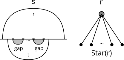
As there are no arcs other than the rainbow, αrsubscript𝛼𝑟\alpha_{r}, we have S(t)={r}𝑆𝑡𝑟S(t)=\{r\}. By construction, b(r)g0(t)𝑏𝑟subscript𝑔0𝑡b(r)\in g_{0}(t) and e(r)gk(t)𝑒𝑟subscript𝑔𝑘𝑡e(r)\in g_{k}(t), the exterior t𝑡t-gaps. We make the Ansatz

G(t)=Star(r)=(R(t),{{r,t}|tT(t)}).𝐺𝑡Star𝑟𝑅𝑡conditional-set𝑟superscript𝑡superscript𝑡𝑇𝑡G(t)=\text{\rm Star}(r)=(R(t),\{\{r,t^{\prime}\}|t^{\prime}\in T(t)\}).

By construction, Star(r)Star𝑟\text{\rm Star}(r) is a connected spanning sub-graph of Gr(t)Gr𝑡\text{\rm Gr}(t). Furthermore, tT(t)for-allsuperscript𝑡𝑇𝑡\forall t^{\prime}\in T(t) we have b(r)<b(t)<b(t)<e(t)<e(t)<e(r)𝑏𝑟𝑏𝑡𝑏superscript𝑡𝑒superscript𝑡𝑒𝑡𝑒𝑟b(r)<b(t)<b(t^{\prime})<e(t^{\prime})<e(t)<e(r). Hence

rtt={b(t),e(t)}𝑟𝑡superscript𝑡𝑏superscript𝑡𝑒superscript𝑡r\cap t\cap t^{\prime}=\{b(t^{\prime}),e(t^{\prime})\}\neq\varnothing

and as a result {r,t,t}K2(R(t))𝑟𝑡superscript𝑡subscript𝐾2𝑅𝑡\{r,t,t^{\prime}\}\in K_{2}(R(t)). Thus, any edge {r,t}E(r)={{r,t}|tT(t)}𝑟superscript𝑡𝐸𝑟conditional-set𝑟superscript𝑡superscript𝑡𝑇𝑡\{r,t^{\prime}\}\in E(r)=\{\{r,t^{\prime}\}|t^{\prime}\in T(t)\} is a ΔtsubscriptΔ𝑡\Delta_{t}-edge and Star(r)Star𝑟\text{\rm Star}(r) is a ΔtsubscriptΔ𝑡\Delta_{t}-graph, establishing the induction basis, see Figure 4.
Refer to caption
Figure 4: LHS: S(t)={r}𝑆𝑡𝑟S(t)=\{r\}, RHS: G(t)=Star(r)𝐺𝑡𝑆𝑡𝑎𝑟𝑟G(t)=Star(r).

Let next S¯¯𝑆\overline{S} denote a secondary structure, having N10𝑁10N-1\geq 0 arcs. By induction hypothesis, for any such bi-secondary structure, R¯=(S¯,T)¯𝑅¯𝑆𝑇\overline{R}=(\overline{S},T) and tT𝑡𝑇t\in T, a ΔtsubscriptΔ𝑡\Delta_{t}-graph exists. We will denote such a graph by G¯(t)¯𝐺𝑡\overline{G}(t).

We shall prove the existence of a ΔtsubscriptΔ𝑡\Delta_{t}-graph as follows: first we identify and then remove a distinguished non-rainbow arc xS𝑥𝑆x\in S. This gives us the bi-secondary structure R¯=(S¯,T)¯𝑅¯𝑆𝑇\overline{R}=(\overline{S},T), for which the induction hypothesis applies, i.e. a ΔtsubscriptΔ𝑡\Delta_{t}-graph G¯(t)¯𝐺𝑡\overline{G}(t) exists. We then reinsert the arc x𝑥x and inspect how to obtain G(t)𝐺𝑡G(t) from G¯(t)¯𝐺𝑡\overline{G}(t).

Let Expt(S)subscriptExp𝑡𝑆\text{\rm Exp}_{t}(S) be the set of non-rainbow S𝑆S-arcs, x𝑥x, having at least one t𝑡t-exposed endpoint, i.e. either b(x)𝑏𝑥b(x) or e(x)𝑒𝑥e(x) are contained in t𝑡t.

Case 111: Expt(S)subscriptExp𝑡𝑆\text{\rm Exp}_{t}(S)\neq\varnothing.

Refer to caption
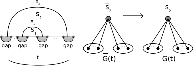
Figure 5: LHS: x1Expt(S)subscript𝑥1subscriptExp𝑡𝑆x_{1}\in\text{\rm Exp}_{t}(S). RHS: the effect of reintroducing x1subscript𝑥1x_{1}, passing from G¯(t)¯𝐺𝑡\overline{G}(t) to G(t)𝐺𝑡G(t).

Select x1Expt(S)subscript𝑥1subscriptExp𝑡𝑆x_{1}\in\text{\rm Exp}_{t}(S). Let s1S(t)subscript𝑠1𝑆𝑡s_{1}\in S(t) be the loop such that x1=αs1subscript𝑥1subscript𝛼subscript𝑠1x_{1}=\alpha_{s_{1}} and let x2subscript𝑥2x_{2} be the arc, that directly covers x1subscript𝑥1x_{1} w.r.t. Ssubscriptprecedes𝑆\prec_{S}. Let s2Ssubscript𝑠2𝑆s_{2}\in S be the loop such that αs2=x2subscript𝛼subscript𝑠2subscript𝑥2\alpha_{s_{2}}=x_{2}. W.l.o.g. we may assume that e(x1)t.𝑒subscript𝑥1𝑡e(x_{1})\in t. Clearly, s2S(t)subscript𝑠2𝑆𝑡s_{2}\in S(t) since e(s1)s2t𝑒subscript𝑠1subscript𝑠2𝑡e(s_{1})\in s_{2}\cap t, see Figure 5.

x1subscript𝑥1x_{1}-removal produces the secondary structure S¯¯𝑆\overline{S} and R¯=(S¯,T)¯𝑅¯𝑆𝑇\overline{R}=(\overline{S},T), for which the induction hypothesis applies. Let s2¯S¯¯subscript𝑠2¯𝑆\overline{s_{2}}\in\overline{S} be such that αs2¯=x2subscript𝛼¯subscript𝑠2subscript𝑥2\alpha_{\overline{s_{2}}}=x_{2}. Then s2¯S¯(t)¯subscript𝑠2¯𝑆𝑡\overline{s_{2}}\in\overline{S}(t) since, in absence of x1subscript𝑥1x_{1}, e(x1)s2¯t𝑒subscript𝑥1¯subscript𝑠2𝑡e(x_{1})\in\overline{s_{2}}\cap t. Hence s2¯¯subscript𝑠2\overline{s_{2}} is a vertex in G¯(t)=(R¯(t),E¯)¯𝐺𝑡¯𝑅𝑡¯𝐸\overline{G}(t)=(\overline{R}(t),\overline{E}).

Reinserting x1subscript𝑥1x_{1} into R¯¯𝑅\overline{R} splits s2¯¯subscript𝑠2\overline{s_{2}} into the two S𝑆S-loops s1subscript𝑠1s_{1} and s2subscript𝑠2s_{2}, see Figure 5.
We make the Ansatz

G(t)=((R¯(t){s2¯}){s1,s2},E),𝐺𝑡¯𝑅𝑡¯subscript𝑠2subscript𝑠1subscript𝑠2𝐸G(t)=((\overline{R}(t)\setminus\{\overline{s_{2}}\})\cup\{s_{1},s_{2}\},E),

where

E𝐸\displaystyle E =\displaystyle= (E¯{{s2¯,r}rR¯(t)}){{s1,s2}}¯𝐸conditional-set¯subscript𝑠2superscript𝑟superscript𝑟¯𝑅𝑡limit-fromsubscript𝑠1subscript𝑠2\displaystyle(\overline{E}\setminus\{\{\overline{s_{2}},r^{\prime}\}\mid r^{\prime}\in\overline{R}(t)\})\cup\{\{s_{1},s_{2}\}\}\cup
{{s1,r}rR(t){s1,s2},s1rt}limit-fromconditional-setsubscript𝑠1superscript𝑟formulae-sequencesuperscript𝑟𝑅𝑡subscript𝑠1subscript𝑠2subscript𝑠1superscript𝑟𝑡\displaystyle\{\{s_{1},r^{\prime}\}\mid r^{\prime}\in R(t)\setminus\{s_{1},s_{2}\},\;s_{1}\cap r^{\prime}\cap t\neq\varnothing\}\cup
{{s2,r}rR(t){s1,s2},s2rt}.conditional-setsubscript𝑠2superscript𝑟formulae-sequencesuperscript𝑟𝑅𝑡subscript𝑠1subscript𝑠2subscript𝑠2superscript𝑟𝑡\displaystyle\{\{s_{2},r^{\prime}\}\mid r^{\prime}\in R(t)\setminus\{s_{1},s_{2}\},\;s_{2}\cap r^{\prime}\cap t\neq\varnothing\}.

Since s2¯=s1s2¯subscript𝑠2subscript𝑠1subscript𝑠2\overline{s_{2}}=s_{1}\cup s_{2} as sets, and R¯(t){s2¯}=R(t){s1,s2}¯𝑅𝑡¯subscript𝑠2𝑅𝑡subscript𝑠1subscript𝑠2\overline{R}(t)\setminus\{\overline{s_{2}}\}=R(t)\setminus\{s_{1},s_{2}\}, we have

{rR¯(t){r,s2¯}E¯}={rR¯(t){s2¯}{r,s1}Eor {r,s2}E}.conditional-setsuperscript𝑟¯𝑅𝑡superscript𝑟¯subscript𝑠2¯𝐸conditional-setsuperscript𝑟¯𝑅𝑡¯subscript𝑠2superscript𝑟subscript𝑠1𝐸or superscript𝑟subscript𝑠2𝐸\{r^{\prime}\in\overline{R}(t)\mid\{r^{\prime},\overline{s_{2}}\}\in\overline{E}\}=\{r^{\prime}\in\overline{R}(t)\setminus\{\overline{s_{2}}\}\mid\{r^{\prime},s_{1}\}\in E\;\text{\rm or }\{r^{\prime},s_{2}\}\in E\}.

Accordingly, any R¯(t)¯𝑅𝑡\overline{R}(t)-vertex connected in G¯(t)¯𝐺𝑡\overline{G}(t) to s2¯¯subscript𝑠2\overline{s_{2}} is, when considered in R(t)𝑅𝑡R(t), connected to either s1subscript𝑠1s_{1} or s2subscript𝑠2s_{2}. In view of {e(x1)}(s1s2t)𝑒subscript𝑥1subscript𝑠1subscript𝑠2𝑡\{e(x_{1})\}\subset(s_{1}\cap\ s_{2}\cap t), we can conclude that s1subscript𝑠1s_{1} and s2subscript𝑠2s_{2} are connected by a ΔtsubscriptΔ𝑡\Delta_{t}-edge. This guarantees that G(t)𝐺𝑡G(t) is a connected spanning sub-graph of Gr(t)Gr𝑡\text{\rm Gr}(t).

Case 222: Expt(S)=subscriptExp𝑡𝑆\text{\rm Exp}_{t}(S)=\varnothing.
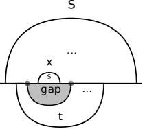
Having no arcs with exposed endpoints, for any loop sS𝑠𝑆s\in S, there exist t𝑡t-gaps, containing b(s)𝑏𝑠b(s) and e(s)𝑒𝑠e(s). Suppose first, there exists an arc x𝑥x having both endpoints in the same gap, see Figure 6. The associated loop, s𝑠s, having αs=xsubscript𝛼𝑠𝑥\alpha_{s}=x, is not contained in S(t)𝑆𝑡S(t). Upon inspection

S¯(t)=S(t)and G(t)=G¯(t),¯𝑆𝑡𝑆𝑡and 𝐺𝑡¯𝐺𝑡\overline{S}(t)=S(t)\;\text{\rm and }G(t)=\overline{G}(t),

Hence the induction hypothesis directly implies the existence of G(t)𝐺𝑡G(t).

Refer to caption
Figure 6: The case where b(x)𝑏𝑥b(x) and e(x)𝑒𝑥e(x) are contained in the same t𝑡t-gap.

It thus remains to discuss S𝑆S-arcs, whose endpoints belong to distinct t𝑡t-gaps, see Figure 7. We shall distinguish the following two scenarios:

(a) (SS(t)){r}𝑆𝑆𝑡𝑟(S\setminus S(t))\setminus\{r\}\neq\varnothing, where αrsubscript𝛼𝑟\alpha_{r} is the rainbow arc.
We shall show that the removal of an arc x=αs,s(SS(t)){r}formulae-sequence𝑥subscript𝛼𝑠𝑠𝑆𝑆𝑡𝑟x=\alpha_{s},s\in(S\setminus S(t))\setminus\{r\}, will not affect G(t)𝐺𝑡G(t), aside from relabeling of a single vertex. Since s1S(t)subscript𝑠1𝑆𝑡s_{1}\notin S(t) we have s2¯S¯(t)¯subscript𝑠2¯𝑆𝑡\overline{s_{2}}\notin\overline{S}(t) if and only if s2S(t)subscript𝑠2𝑆𝑡s_{2}\notin S(t). In this case we set G(t)=G¯(t)𝐺𝑡¯𝐺𝑡G(t)=\overline{G}(t) and the assertion is directly implied by the induction hypothesis. In case of s2¯S¯(t)¯subscript𝑠2¯𝑆𝑡\overline{s_{2}}\in\overline{S}(t), G(t)𝐺𝑡G(t) is obtained from G¯(t)¯𝐺𝑡\overline{G}(t) by relabeling s2¯¯subscript𝑠2\overline{s_{2}} to s2subscript𝑠2s_{2} exhibiting no other changes, see Figure 7:

G(t)=((R¯(t){s2¯}){s2},E),𝐺𝑡¯𝑅𝑡¯subscript𝑠2subscript𝑠2𝐸G(t)=((\overline{R}(t)\setminus\{\overline{s_{2}}\})\cup\{s_{2}\},E),

where

E=(E¯{{s2¯,r}E¯rR¯(t)}){{s2,r}rR¯(t),{s2¯,r}E¯}𝐸¯𝐸conditional-set¯subscript𝑠2superscript𝑟¯𝐸superscript𝑟¯𝑅𝑡conditional-setsubscript𝑠2superscript𝑟formulae-sequencesuperscript𝑟¯𝑅𝑡¯subscript𝑠2superscript𝑟¯𝐸E=(\overline{E}\setminus\{\{\overline{s_{2}},r^{\prime}\}\in\overline{E}\mid r^{\prime}\in\overline{R}(t)\})\cup\{\{s_{2},r^{\prime}\}\mid r^{\prime}\in\overline{R}(t),\{\overline{s_{2}},r^{\prime}\}\in\overline{E}\}

and G(t)𝐺𝑡G(t) is consequently a ΔtsubscriptΔ𝑡\Delta_{t}-graph.

Refer to caption
Figure 7: LHS: all S𝑆S-arcs having their endpoints in distinct t𝑡t-gaps. RHS: (a)𝑎(a), s2¯S¯(t)¯subscript𝑠2¯𝑆𝑡\overline{s_{2}}\in\overline{S}(t), G(t)𝐺𝑡G(t) is obtained by a relabelling of G¯(t)¯𝐺𝑡\overline{G}(t).

(b) (SS(t)){r}=𝑆𝑆𝑡𝑟(S\setminus S(t))\setminus\{r\}=\varnothing, where αrsubscript𝛼𝑟\alpha_{r} is the rainbow arc.
We then have either SS(t)=𝑆𝑆𝑡S\setminus S(t)=\varnothing or SS(t)={r}𝑆𝑆𝑡𝑟S\setminus S(t)=\{r\}. In the latter case we select x𝑥x to be an arc, corresponding to a loop s1subscript𝑠1s_{1}, that is immediately covered by αrsubscript𝛼𝑟\alpha_{r}. Let s2=rsubscript𝑠2𝑟s_{2}=r. Since rS(t)𝑟𝑆𝑡r\notin S(t) we make the Ansatz

G(t)=((R¯(t){s2¯}){s1},E),𝐺𝑡¯𝑅𝑡¯subscript𝑠2subscript𝑠1𝐸G(t)=((\overline{R}(t)\setminus\{\overline{s_{2}}\})\cup\{s_{1}\},E),

where

E=(E¯{{s2¯,r}E¯rR¯(t)}){{s1,r}rR¯(t),{s2¯,r}E¯}.𝐸¯𝐸conditional-set¯subscript𝑠2superscript𝑟¯𝐸superscript𝑟¯𝑅𝑡conditional-setsubscript𝑠1superscript𝑟formulae-sequencesuperscript𝑟¯𝑅𝑡¯subscript𝑠2superscript𝑟¯𝐸E=(\overline{E}\setminus\{\{\overline{s_{2}},r^{\prime}\}\in\overline{E}\mid r^{\prime}\in\overline{R}(t)\})\cup\{\{s_{1},r^{\prime}\}\mid r^{\prime}\in\overline{R}(t),\{\overline{s_{2}},r^{\prime}\}\in\overline{E}\}.

Accordingly, G(t)𝐺𝑡G(t) is obtained from G¯(t)¯𝐺𝑡\overline{G}(t) by relabeling s2¯¯subscript𝑠2\overline{s_{2}} by s1subscript𝑠1s_{1} and G(t)𝐺𝑡G(t) is a ΔtsubscriptΔ𝑡\Delta_{t}-graph, see Figure 8.

It remains to analyze SS(t)=𝑆𝑆𝑡S\setminus S(t)=\varnothing, i.e. all S𝑆S-arcs are contained in S(t)𝑆𝑡S(t), where we recall we reduced the analysis to arcs whose endpoints belong to different t𝑡t-gaps.

Refer to caption
Figure 8: LHS: the case SS(t)={r}𝑆𝑆𝑡𝑟S\setminus S(t)=\{r\}. RHS: the case SS(t)=𝑆𝑆𝑡S\setminus S(t)=\varnothing.

Suppose now all S𝑆S-loops are contained in S(t)𝑆𝑡S(t). Consider the set of all minimal arcs of S𝑆S w.r.t. Ssubscriptprecedes𝑆\prec_{S}. We claim there exists one such minimal arc, call it αs1subscript𝛼subscript𝑠1\alpha_{s_{1}}, such that its immediate cover w.r.t. Ssubscriptprecedes𝑆\prec_{S}, call it αs2subscript𝛼subscript𝑠2\alpha_{s_{2}}, is such that s2subscript𝑠2s_{2} contains at least one of the endpoints of one of the t𝑡t-gaps that contain one of the endpoints of αs1subscript𝛼subscript𝑠1\alpha_{s_{1}}. To show this we observe that if all t𝑡t-gaps would have their endpoints inside loops corresponding to Ssubscriptprecedes𝑆\prec_{S}-minimal arcs, then at least one arc that immediately covers such minimal arcs would not correspond to a loop in S(t)𝑆𝑡S(t). Hence, there must be a loop s1subscript𝑠1s_{1} with αs1subscript𝛼subscript𝑠1\alpha_{s_{1}} minimal w.r.t. Ssubscriptprecedes𝑆\prec_{S} and an arc αs2subscript𝛼subscript𝑠2\alpha_{s_{2}} that immediately covers αs1subscript𝛼subscript𝑠1\alpha_{s_{1}}, such that s2subscript𝑠2s_{2} contains one of the endpoints of a gap that contains b(s1)𝑏subscript𝑠1b(s_{1}) or e(s1)𝑒subscript𝑠1e(s_{1}).

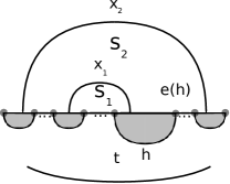
Let us denote this gap by hh. W.l.o.g. we can assume e(s1)h𝑒subscript𝑠1e(s_{1})\in h, see Figure 9. Then, the minimality of s1subscript𝑠1s_{1} guarantees that s1subscript𝑠1s_{1} contains the other endpoint of the gap hh. We shall now remove x1=αs1subscript𝑥1subscript𝛼subscript𝑠1x_{1}=\alpha_{s_{1}}.

Refer to caption
Figure 9: x1=αs1subscript𝑥1subscript𝛼subscript𝑠1x_{1}=\alpha_{s_{1}} is minimal w.r.t. Ssubscriptprecedes𝑆\prec_{S}.

We consider the loop tsuperscript𝑡t^{\prime} associated to hh and note that s1ttsubscript𝑠1superscript𝑡𝑡s_{1}\cap t^{\prime}\cap t\neq\varnothing as well as s2ttsubscript𝑠2superscript𝑡𝑡s_{2}\cap t^{\prime}\cap t\neq\varnothing. Accordingly, tsuperscript𝑡t^{\prime} connects s1,s2subscript𝑠1subscript𝑠2s_{1},s_{2} in R(t)𝑅𝑡R(t) by means of ΔtsubscriptΔ𝑡\Delta_{t}-edges, see Figure 8 and we immediately obtain that

G(t)=((R¯(t){s2¯}){s1,s2},E),𝐺𝑡¯𝑅𝑡¯subscript𝑠2subscript𝑠1subscript𝑠2𝐸G(t)=((\overline{R}(t)\setminus\{\overline{s_{2}}\})\cup\{s_{1},s_{2}\},E),

where

E𝐸\displaystyle E =\displaystyle= (E¯{{s2¯,r}E¯rR¯(t)})limit-from¯𝐸conditional-set¯subscript𝑠2superscript𝑟¯𝐸superscript𝑟¯𝑅𝑡\displaystyle(\overline{E}\setminus\{\{\overline{s_{2}},r^{\prime}\}\in\overline{E}\mid r^{\prime}\in\overline{R}(t)\})\cup
{{s1,r}rR(t),s1rt}limit-fromconditional-setsubscript𝑠1superscript𝑟formulae-sequencesuperscript𝑟𝑅𝑡subscript𝑠1superscript𝑟𝑡\displaystyle\{\{s_{1},r^{\prime}\}\mid r^{\prime}\in R(t),s_{1}\cap r^{\prime}\cap t\neq\varnothing\}\cup
{{s2,r}rR(t),s2rt},conditional-setsubscript𝑠2superscript𝑟formulae-sequencesuperscript𝑟𝑅𝑡subscript𝑠2superscript𝑟𝑡\displaystyle\{\{s_{2},r^{\prime}\}\mid r^{\prime}\in R(t),s_{2}\cap r^{\prime}\cap t\neq\varnothing\},

is a ΔtsubscriptΔ𝑡\Delta_{t}-graph for R(t)𝑅𝑡R(t). This concludes the proof of the induction step and the lemma follows. ∎

Next we compute H2(R)subscript𝐻2𝑅H_{2}(R),

Theorem 3.

For any bi-secondary structure, R=(S,T)𝑅𝑆𝑇R=(S,T), with loop nerve K(R)𝐾𝑅K(R), we have

H2(R)i=1k,subscript𝐻2𝑅superscriptsubscriptdirect-sum𝑖1𝑘H_{2}(R)\cong\bigoplus_{i=1}^{k}\mathbb{Z},

i.e. H2(R)subscript𝐻2𝑅H_{2}(R) is free of finite rank.

Proof.

Claim 111. Im(3)C3(R)Imsubscript3subscript𝐶3𝑅\text{\rm Im}(\partial_{3})\cong C_{3}(R), i.e. Im(3)Imsubscript3\text{\rm Im}(\partial_{3}) is a free Abelian group and freely generated by P={3(Yi)Yiis a 3-simplex}𝑃conditional-setsubscript3subscript𝑌𝑖subscript𝑌𝑖is a 3-simplexP=\{\partial_{3}(Y_{i})\mid Y_{i}\;\text{\rm is a $3$-simplex}\}.

Claim 111 is a consequence of two facts: (a) C4(R)=0subscript𝐶4𝑅0C_{4}(R)=0 and (b) H3(R)=0subscript𝐻3𝑅0H_{3}(R)=0, both of which we prove below. It is obtained as follows: C4(R)=0subscript𝐶4𝑅0C_{4}(R)=0 guarantees Im(4)=0Imsubscript40\text{\rm Im}(\partial_{4})=0, which in view of 0=H3(R)=Ker(3)/Im(4)0subscript𝐻3𝑅Kersubscript3Imsubscript40=H_{3}(R)=\text{\rm Ker}(\partial_{3})/\text{\rm Im}(\partial_{4}) implies Ker(3)=0Kersubscript30\text{\rm Ker}(\partial_{3})=0. This in turn implies that 3subscript3\partial_{3} is an embedding, i.e. Im(3)C3(R)Imsubscript3subscript𝐶3𝑅\text{\rm Im}(\partial_{3})\cong C_{3}(R), whence Im(3)Imsubscript3\text{\rm Im}(\partial_{3}) is a free Abelian group. P𝑃P certainly generates Im(3)Imsubscript3\text{\rm Im}(\partial_{3}) and a \mathbb{Z}-linear combination

jλj3(Yj)=3(jλjYj)=0subscript𝑗subscript𝜆𝑗subscript3subscript𝑌𝑗subscript3subscript𝑗subscript𝜆𝑗subscript𝑌𝑗0\sum_{j}\lambda_{j}\partial_{3}(Y_{j})=\partial_{3}(\sum_{j}\lambda_{j}Y_{j})=0

means that jλjYjKer(3)subscript𝑗subscript𝜆𝑗subscript𝑌𝑗Kersubscript3\sum_{j}\lambda_{j}Y_{j}\in\text{\rm Ker}(\partial_{3}). Since the latter is trivial we arrive at

jλjYj=0subscript𝑗subscript𝜆𝑗subscript𝑌𝑗0\sum_{j}\lambda_{j}Y_{j}=0

which implies λj=0subscript𝜆𝑗0\lambda_{j}=0, for any j𝑗j appearing in this sum. This shows that the P𝑃P-elements are \mathbb{Z}-linear independent.

Let YiK3(R)subscript𝑌𝑖subscript𝐾3𝑅Y_{i}\in K_{3}(R), 0ik0𝑖𝑘0\leq i\leq k denote the generators of C3(R)subscript𝐶3𝑅C_{3}(R). Lemma 4 guarantees that each 333-simplex Y𝑌Y has at least two Y𝑌Y-exposed 222-faces. Hence, to each generator YiK3(R)subscript𝑌𝑖subscript𝐾3𝑅Y_{i}\in K_{3}(R) there correspond at least two generators of the free group C2(R)subscript𝐶2𝑅C_{2}(R) that appear as terms only in the image 3(Yi)subscript3subscript𝑌𝑖\partial_{3}(Y_{i}). Let us write

3(Yi)=u(i)Uu(i)+c(i)Cc(i),subscript3subscript𝑌𝑖subscript𝑢𝑖subscript𝑈𝑢𝑖subscript𝑐𝑖subscript𝐶𝑐𝑖\partial_{3}(Y_{i})=\sum_{u(i)}U_{u(i)}+\sum_{c(i)}C_{c(i)},

distinguishing exposed, signed and covered, signed 222-faces of Yisubscript𝑌𝑖Y_{i}, i.e. we consider the sign, induced by the boundary map, to be part of Uu(i)subscript𝑈𝑢𝑖U_{u(i)} and Cc(i)subscript𝐶𝑐𝑖C_{c(i)}, respectively. In particular, for any u(i)𝑢𝑖u(i), there exists an unique r𝑟r, such that we have either Uu(i)=+Zrsubscript𝑈𝑢𝑖subscript𝑍𝑟U_{u(i)}=+Z_{r} or Uu(i)=Zrsubscript𝑈𝑢𝑖subscript𝑍𝑟U_{u(i)}=-Z_{r} where Zrsubscript𝑍𝑟Z_{r} is a generator of C2(R)subscript𝐶2𝑅C_{2}(R).

Claim 222. C2(R)/Im(3)subscript𝐶2𝑅Imsubscript3C_{2}(R)/\text{\rm Im}(\partial_{3}) is free.

We consider C2(R)¯=C2(R)/Im(3)¯subscript𝐶2𝑅subscript𝐶2𝑅Imsubscript3\overline{C_{2}(R)}=C_{2}(R)/\text{\rm Im}(\partial_{3}) as a \mathbb{Z}-module and suppose X𝑋X is a torsion element of order n𝑛n in C2(R)¯¯subscript𝐶2𝑅\overline{C_{2}(R)}. Then we can represent X𝑋X as

X=rλrZr+Im(3),𝑋subscript𝑟subscript𝜆𝑟subscript𝑍𝑟Imsubscript3X=\sum_{r}\lambda_{r}Z_{r}+\text{\rm Im}(\partial_{3}),

where, w.l.o.g. we assume that all λr0subscript𝜆𝑟0\lambda_{r}\neq 0. Since X𝑋X is a torsion element, we have nX=0𝑛𝑋0nX=0 in C2(R)¯¯subscript𝐶2𝑅\overline{C_{2}(R)}, i.e.

n(rλrZr)𝑛subscript𝑟subscript𝜆𝑟subscript𝑍𝑟\displaystyle n(\sum_{r}\lambda_{r}Z_{r}) =\displaystyle= i=1kαi3(Yi)superscriptsubscript𝑖1𝑘subscript𝛼𝑖subscript3subscript𝑌𝑖\displaystyle\sum_{i=1}^{k}\alpha_{i}\partial_{3}(Y_{i})
=\displaystyle= i=1αi(u(i)Uu(i))+i=1αi(c(i)Cc(i))subscript𝑖1subscript𝛼𝑖subscript𝑢𝑖subscript𝑈𝑢𝑖subscript𝑖1subscript𝛼𝑖subscript𝑐𝑖subscript𝐶𝑐𝑖\displaystyle\sum_{i=1}\alpha_{i}(\sum_{u(i)}U_{u(i)})+\sum_{i=1}\alpha_{i}(\sum_{c(i)}C_{c(i)})

where λr,αisubscript𝜆𝑟subscript𝛼𝑖\lambda_{r},\alpha_{i}\in\mathbb{Z} are unique nonzero integer coefficients. Clearly, each unique signed 222-face, Uu(i)subscript𝑈𝑢𝑖U_{u(i)} of the RHS corresponds to a unique generator Zr(Uu(i))subscript𝑍𝑟subscript𝑈𝑢𝑖Z_{r(U_{u(i)})} and hence, irrespective of the particular choice of the u(i)𝑢𝑖u(i) and the sign of Uu(i)subscript𝑈𝑢𝑖U_{u(i)}, we obtain for any i𝑖i of the sum on the RHS

nλr(Uu(i))=αi,𝑛subscript𝜆𝑟subscript𝑈𝑢𝑖subscript𝛼𝑖n\lambda_{r(U_{u(i)})}=\alpha_{i},

only depending on the index i𝑖i. This is an equation in \mathbb{Z} and hence implies αi0modnsubscript𝛼𝑖modulo0𝑛\alpha_{i}\equiv 0\mod n. Accordingly, we derive

(rλrZr)=i=1kαin3(Yi),subscript𝑟subscript𝜆𝑟subscript𝑍𝑟superscriptsubscript𝑖1𝑘subscript𝛼𝑖𝑛subscript3subscript𝑌𝑖(\sum_{r}\lambda_{r}Z_{r})=\sum_{i=1}^{k}\frac{\alpha_{i}}{n}\partial_{3}(Y_{i}),

which means XIm(3)𝑋Imsubscript3X\in\text{\rm Im}(\partial_{3}), since αinsubscript𝛼𝑖𝑛\frac{\alpha_{i}}{n}\in\mathbb{Z}, i.e. X=0𝑋0X=0. By transposition we have proved that X0𝑋0X\neq 0 in C2(R)¯¯subscript𝐶2𝑅\overline{C_{2}(R)} implies for any n𝑛n\in\mathbb{N}, nX0𝑛𝑋0nX\neq 0 in C2(R)¯¯subscript𝐶2𝑅\overline{C_{2}(R)}, whence C2(R)¯¯subscript𝐶2𝑅\overline{C_{2}(R)} is free and Claim 222 is proved.

As a result, Ker(2)/Im(3)Kersubscript2Imsubscript3\text{\rm Ker}(\partial_{2})/\text{\rm Im}(\partial_{3}) is, as a subgroup of the free group C2(R)¯¯subscript𝐶2𝑅\overline{C_{2}(R)}, itself free and the theorem is proved. ∎

It remains to show Cd(R)=0subscript𝐶𝑑𝑅0C_{d}(R)=0 for d4𝑑4d\geq 4 and H3(R)=0subscript𝐻3𝑅0H_{3}(R)=0.

Lemma 7.

Let R=(S,T)𝑅𝑆𝑇R=(S,T) be a bi-secondary structure with loop-nerve K(R)𝐾𝑅K(R) and let d4𝑑4d\geq 4, then Kd(R)=subscript𝐾𝑑𝑅K_{d}(R)=\varnothing, Cd(R)=0subscript𝐶𝑑𝑅0C_{d}(R)=0 and Hd(R)=0subscript𝐻𝑑𝑅0H_{d}(R)=0.

Proof.

For any Y={ri0,,rid}Kd(R)𝑌subscript𝑟subscript𝑖0subscript𝑟subscript𝑖𝑑subscript𝐾𝑑𝑅Y=\{r_{i_{0}},\ldots,r_{i_{d}}\}\in K_{d}(R) for some d4𝑑4d\geq 4 we have Ω(Y)=k=0drikΩ𝑌superscriptsubscript𝑘0𝑑subscript𝑟subscript𝑖𝑘\Omega(Y)=\bigcap_{k=0}^{d}r_{i_{k}}\neq\varnothing. Since d4𝑑4d\geq 4, |Y|5𝑌5|Y|\geq 5, whence at least three loops r0,r1,r2Ysubscriptsuperscript𝑟0subscriptsuperscript𝑟1subscriptsuperscript𝑟2𝑌r^{\prime}_{0},r^{\prime}_{1},r^{\prime}_{2}\in Y are contained in the same secondary structure, which is a contradiction to Proposition 1, which stipulates that three loops of one secondary structure intersect only trivially. ∎

Next we show that H3(R)=0subscript𝐻3𝑅0H_{3}(R)=0.

Theorem 4.

Let R=(S,T)𝑅𝑆𝑇R=(S,T) be a bi-secondary structure with loop nerve K(R)𝐾𝑅K(R), then H3(R)=0subscript𝐻3𝑅0H_{3}(R)=0.

Proof.

Consider

X=YiK3(R)niYiC3(R)Ker(3),𝑋subscriptsubscript𝑌𝑖subscript𝐾3𝑅subscript𝑛𝑖subscript𝑌𝑖subscript𝐶3𝑅Kersubscript3X=\sum_{Y_{i}\in K_{3}(R)}n_{i}Y_{i}\in C_{3}(R)\in\text{\rm Ker}(\partial_{3}),

then

3(X)subscript3𝑋\displaystyle\partial_{3}(X) =\displaystyle= YiK3(R)ni3(Yi)subscriptsubscript𝑌𝑖subscript𝐾3𝑅subscript𝑛𝑖subscript3subscript𝑌𝑖\displaystyle\sum_{Y_{i}\in K_{3}(R)}n_{i}\partial_{3}(Y_{i})
=\displaystyle= ini(u(i)Uu(i))+ini(c(i)Cc(i)),subscript𝑖subscript𝑛𝑖subscript𝑢𝑖subscript𝑈𝑢𝑖subscript𝑖subscript𝑛𝑖subscript𝑐𝑖subscript𝐶𝑐𝑖\displaystyle\sum_{i}n_{i}(\sum_{u(i)}U_{u(i)})+\sum_{i}n_{i}(\sum_{c(i)}C_{c(i)}),

where the Uu(i)subscript𝑈𝑢𝑖U_{u(i)} and Cc(i)subscript𝐶𝑐𝑖C_{c(i)} are the signed exposed and covered 222-faces of Yisubscript𝑌𝑖Y_{i}, respectively. Since we have at least two unique exposed 222-faces and, by assumption, 3(X)=0subscript3𝑋0\partial_{3}(X)=0, we conclude that for any i𝑖i of X=YiK3(R)niYi𝑋subscriptsubscript𝑌𝑖subscript𝐾3𝑅subscript𝑛𝑖subscript𝑌𝑖X=\sum_{Y_{i}\in K_{3}(R)}n_{i}Y_{i} we have ni=0subscript𝑛𝑖0n_{i}=0. Therefore X=0𝑋0X=0 and Ker(3)Kersubscript3\text{\rm Ker}(\partial_{3}) contains no nontrivial elements, whence H3(R)=0subscript𝐻3𝑅0H_{3}(R)=0. ∎

4 Discussion

In the previous section, we showed that H2(R)subscript𝐻2𝑅H_{2}(R) is non-trivial and free, leading to a novel observable for the pair of secondary structures (S,T)𝑆𝑇(S,T), namely the rank of H2(R=(S,T))subscript𝐻2𝑅𝑆𝑇H_{2}(R=(S,T)), r(H2(R))𝑟subscript𝐻2𝑅r(H_{2}(R)). We shall see that the generators of r(H2(R))𝑟subscript𝐻2𝑅r(H_{2}(R)) represent key information about the “switching sequence” [42], a segment of the sequence, that engages w.r.t. each respective structure in a distinct, mutually exclusive fashion.

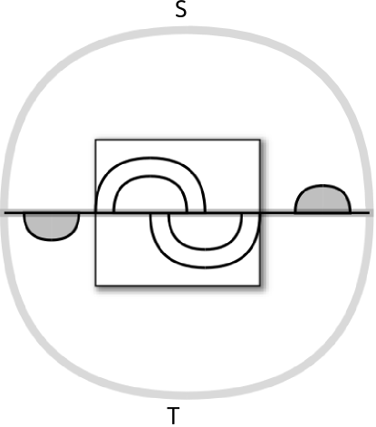
It is well known from experimental work that native riboswitch pairs, ncRNAs, exhibit two distinct, mutually exclusive, stable secondary structures [43]. We analyzed all nine riboswitch sequences contained in the Swispot database [44] and observed that r(H2(R))=1𝑟subscript𝐻2𝑅1r(H_{2}(R))=1. In Figure  10 we illustrate the connection between a H2(R)subscript𝐻2𝑅H_{2}(R)-generator and pairs of mutually exclusive substructures.
Refer to caption
Figure 10: H2(R)subscript𝐻2𝑅H_{2}(R)-generators and mutually exclusive structure pairs: the two helices (boxed) are mutually exclusive, while the two substructures (shaded) are not. The former two, together with the two rainbows correspond to a generator of H2(R)subscript𝐻2𝑅H_{2}(R).

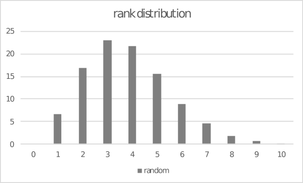
The ranks, r(H2(R))𝑟subscript𝐻2𝑅r(H_{2}(R)), for uniformly sampled structures pairs, are displayed in Figure  11, showing that 6.7%percent6.76.7\% of the uniform random pairs exhibit r(H2(R))=1𝑟subscript𝐻2𝑅1r(H_{2}(R))=1.

Refer to caption
Figure 11: r(H2(R))𝑟subscript𝐻2𝑅r(H_{2}(R)) for uniformly random structure pairs: r(H2(R))𝑟subscript𝐻2𝑅r(H_{2}(R)) (x𝑥x-axis) and the relative frequencies (y𝑦y-axis).

As for future work, the complexity analysis and optimal scheduling problems arising from the work of Huang [41] suggest to consider a graded version of the homologies, developed here. Let t1𝑡1t\geq 1 be an integer and R=(S,T)𝑅𝑆𝑇R=(S,T) be a bi-secondary structure. We set Kdt(R)={YKd(R)|ω(Y)t}superscriptsubscript𝐾𝑑𝑡𝑅conditional-set𝑌subscript𝐾𝑑𝑅𝜔𝑌𝑡K_{d}^{t}(R)=\{Y\in K_{d}(R)|\omega(Y)\geq t\}, the set of d𝑑d-simplices of weight at least t𝑡t. We define Cdt(R)superscriptsubscript𝐶𝑑𝑡𝑅C_{d}^{t}(R) to be the free abelian group generated by Kdt(R)superscriptsubscript𝐾𝑑𝑡𝑅K_{d}^{t}(R), i.e. the chain group of rank d𝑑d and weight at least t𝑡t. It is easy to see then that Cd(R)=Cd1(R)subscript𝐶𝑑𝑅superscriptsubscript𝐶𝑑1𝑅C_{d}(R)=C_{d}^{1}(R) for all d0𝑑0d\geq 0 and that Cdt+1(R)Cdt(R)superscriptsubscript𝐶𝑑𝑡1𝑅superscriptsubscript𝐶𝑑𝑡𝑅C_{d}^{t+1}(R)\leq C_{d}^{t}(R) for all t1𝑡1t\geq 1 and all d0𝑑0d\geq 0. We can naturally define boundary operators for these groups in terms of restrictions of our original boundary maps as dt:Cdt(R)Cd1t(R):superscriptsubscript𝑑𝑡absentsuperscriptsubscript𝐶𝑑𝑡𝑅superscriptsubscript𝐶𝑑1𝑡𝑅\partial_{d}^{t}:C_{d}^{t}(R)\xrightarrow[]{}C_{d-1}^{t}(R) with dt=d|Cdt(R)superscriptsubscript𝑑𝑡evaluated-atsubscript𝑑superscriptsubscript𝐶𝑑𝑡𝑅\partial_{d}^{t}=\partial_{d}|_{C_{d}^{t}(R)}. As such, we obtain a t𝑡t-parametric sequence of nerves {Kt(R)}t1subscriptsuperscript𝐾𝑡𝑅𝑡1\{K^{t}(R)\}_{t\geq 1} each of which gives rise to its t𝑡t-labelled homology sequence. Tracking the persistence of homology group generators across the newly obtained homological t𝑡t-spectrum gives rise to a more granular analysis of the structure of the complete nerve [45]. This analysis represents a version of persistent homology, pioneered by Edelsbrunner and by Gunnar Carlson [46, 47, 48] and is of central importance for designing an optimal loop-removal schedule in [41].

We extend the homology analysis to planar interaction structures [49]. Due to the fact that the physical 53superscript5superscript35^{\prime}-3^{\prime} distance for RNA𝑅𝑁𝐴RNA strands is in general very small [50], the formation of an interaction structure is connected to the alignment of two discs, each representing the respective, circular backbone. That is, interpreting the two circles corresponding to two interacting secondary structures S1,S2subscript𝑆1subscript𝑆2S_{1},S_{2} to be (D(0,1))𝐷01\partial(D(0,1)), the boundaries of unit disks in \mathbb{C}. These boundaries contain distinguished points that correspond to the paired vertices in the secondary structures. The connection between interaction structure and disc-alignment leads one to consider one disc being acted upon by Möbius transforms. This action is well defined since the Möbius maps of the disc map the boundary to itself and, being holomorphic, cannot introduce crossings. Different alignments are then captured by these automorphisms and give rise to a spectrum of homologies, as introduced in this paper.

5 Declarations of interest

None.

6 Acknowledgments

We gratefully acknowledge the comments from Fenix Huang. Many thanks to Thomas Li, Ricky Chen and Reza Rezazadegan for discussions.

References

References

  • [1] J. E. Darnell, RNA: life’s indispensable molecule, Cold Spring Harbor Laboratory Press New York, 2011.
  • [2] R. W. Holley, J. Apgar, G. A. Everett, J. T. Madison, M. Marquisee, S. H. Merrill, J. R. Penswick, A. Zamir, Structure of a ribonucleic acid, Science (1965) 1462–1465.
  • [3] D. Thirumalai, N. Lee, S. A. Woodson, D. Klimov, Early events in rna folding, Annual review of physical chemistry 52 (1) (2001) 751–762.
  • [4] J. R. Fresco, B. M. Alberts, P. Doty, et al., Some molecular details of the secondary structure of ribonucleic acid., Nature 188 (1960) 98–101.
  • [5] J. Gralla, D. M. Crothers, Free energy of imperfect nucleic acid helices: Ii. small hairpin loops, Journal of molecular biology 73 (4) (1973) 497–511.
  • [6] D. H. Turner, D. H. Mathews, Nndb: the nearest neighbor parameter database for predicting stability of nucleic acid secondary structure, Nucleic acids research 38 (suppl_1) (2009) D280–D282.
  • [7] J. M. Pipas, J. E. McMAHON, Method for predicting rna secondary structure, Proceedings of the National Academy of Sciences 72 (6) (1975) 2017–2021.
  • [8] C. Delisi, D. M. Crothers, Prediction of rna secondary structure, Proceedings of the National Academy of Sciences 68 (11) (1971) 2682–2685.
  • [9] I. Tinoco, O. C. Uhlenbeck, M. D. Levine, Estimation of secondary structure in ribonucleic acids, Nature 230 (5293) (1971) 362.
  • [10] M. S. Waterman, Secondary structure of single-stranded nucleic acids, Adv. math. suppl. studies 1 (1978) 167–212.
  • [11] R. Nussinov, A. B. Jacobson, Fast algorithm for predicting the secondary structure of single-stranded rna, Proceedings of the National Academy of Sciences 77 (11) (1980) 6309–6313.
  • [12] M. S. Waterman, T. F. Smith, Rapid dynamic programming algorithms for rna secondary structure, Advances in Applied Mathematics 7 (4) (1986) 455–464.
  • [13] M. Zuker, D. Sankoff, Rna secondary structures and their prediction, Bulletin of mathematical biology 46 (4) (1984) 591–621.
  • [14] J. S. McCaskill, The equilibrium partition function and base pair binding probabilities for rna secondary structure, Biopolymers: Original Research on Biomolecules 29 (6-7) (1990) 1105–1119.
  • [15] C. Haslinger, P. F. Stadler, Rna structures with pseudo-knots: Graph-theoretical, combinatorial, and statistical properties, Bulletin of mathematical biology 61 (3) (1999) 437–467.
  • [16] M. Taufer, A. Licon, R. Araiza, D. Mireles, F. Van Batenburg, A. P. Gultyaev, M.-Y. Leung, Pseudobase++: an extension of pseudobase for easy searching, formatting and visualization of pseudoknots, Nucleic acids research 37 (suppl_1) (2008) D127–D135.
  • [17] C. M. Reidys, Random induced subgraphs of generalizedn-cubes, Advances in Applied Mathematics 19 (3) (1997) 360–377.
  • [18] C. Flamm, I. L. Hofacker, S. Maurer-Stroh, P. F. Stadler, M. Zehl, Design of multistable rna molecules, Rna 7 (2) (2001) 254–265.
  • [19] A. Busch, R. Backofen, Info-rna?a fast approach to inverse rna folding, Bioinformatics 22 (15) (2006) 1823–1831.
  • [20] A. Levin, M. Lis, Y. Ponty, C. W. O?donnell, S. Devadas, B. Berger, J. Waldispühl, A global sampling approach to designing and reengineering rna secondary structures, Nucleic acids research 40 (20) (2012) 10041–10052.
  • [21] C. Barrett, Q. He, F. W. Huang, C. M. Reidys, An efficient dual sampling algorithm with hamming distance filtration, Journal of Computational Biology 25 (11) (2018) 1179–1192.
  • [22] C. Barrett, F. W. Huang, C. M. Reidys, Sequence–structure relations of biopolymers, Bioinformatics 33 (3) (2017) 382–389.
  • [23] Q. He, F. W. Huang, C. Barrett, C. M. Reidys, Genetic robustness of let-7 mirna sequence-structure pairs, arXiv preprint arXiv:1801.05056.
  • [24] W. R. Schmitt, M. S. Waterman, Linear trees and rna secondary structure, Discrete Applied Mathematics 51 (3) (1994) 317–323.
  • [25] I. L. Hofacker, P. Schuster, P. F. Stadler, Combinatorics of rna secondary structures, Discrete Applied Mathematics 88 (1-3) (1998) 207–237.
  • [26] E. Y. Jin, J. Qin, C. M. Reidys, Combinatorics of rna structures with pseudoknots, Bulletin of mathematical biology 70 (1) (2008) 45–67.
  • [27] H. Orland, A. Zee, Rna folding and large n matrix theory, Nuclear Physics B 620 (3) (2002) 456–476.
  • [28] J. E. Andersen, L. O. Chekhov, R. Penner, C. M. Reidys, P. Sułkowski, Topological recursion for chord diagrams, rna complexes, and cells in moduli spaces, Nuclear Physics B 866 (3) (2013) 414–443.
  • [29] M. Bon, G. Vernizzi, H. Orland, A. Zee, Topological classification of rna structures, Journal of molecular biology 379 (4) (2008) 900–911.
  • [30] J. E. Andersen, R. C. Penner, C. M. Reidys, M. S. Waterman, Topological classification and enumeration of rna structures by genus, Journal of mathematical biology 67 (5) (2013) 1261–1278.
  • [31] F. W. Huang, C. M. Reidys, Shapes of topological rna structures, Mathematical biosciences 270 (2015) 57–65.
  • [32] W. Chen, E. Deng, R. Du, R. Stanley, C. Yan, Crossings and nestings of matchings and partitions, Transactions of the American Mathematical Society 359 (4) (2007) 1555–1575.
  • [33] R. P. Stanley, Enumerative combinatorics, wadsworth publ, Co., Belmont, CA.
  • [34] S. Sundaram, The cauchy identity for sp (2n).
  • [35] R. Penner, M. S. Waterman, Spaces of rna secondary structures, Advances in Mathematics 101 (1) (1993) 31–49.
  • [36] J. Harer, D. Zagier, The euler characteristic of the moduli space of curves, Inventiones mathematicae 85 (3) (1986) 457–485.
  • [37] J. Ambjørn, L. Chekhov, C. F. Kristjansen, Y. Makeenko, Matrix model calculations beyond the spherical limit, Nuclear Physics B 404 (1-2) (1993) 127–172.
  • [38] G. Chapuy, A new combinatorial identity for unicellular maps, via a direct bijective approach, Advances in Applied Mathematics 47 (4) (2011) 874–893.
  • [39] F. W. Huang, C. M. Reidys, Topological language for rna, Mathematical biosciences 282 (2016) 109–120.
  • [40] C. M. Reidys, Neutral networks of rna secondary structures.
  • [41] F. W. Huang, Personal Communication.
  • [42] R. R. Breaker, Riboswitches and the rna world, Cold Spring Harbor perspectives in biology 4 (2) (2012) a003566.
  • [43] A. Serganov, E. Nudler, A decade of riboswitches, Cell 152 (1-2) (2013) 17–24.
  • [44] M. Barsacchi, E. M. Novoa, M. Kellis, A. Bechini, Swispot: modeling riboswitches by spotting out switching sequences, Bioinformatics 32 (21) (2016) 3252–3259.
  • [45] A. Zomorodian, G. Carlsson, Computing persistent homology, Discrete & Computational Geometry 33 (2) (2005) 249–274.
  • [46] H. Edelsbrunner, D. Letscher, A. Zomorodian, Topological persistence and simplification, Discrete & Computational Geometry 28 (4) (2002) 511–533.
  • [47] G. Carlsson, Topology and data, Bull. Amer. Math. Soc. 46 (2009) 255–308.
  • [48] G. Carlsson, A. Zomorodian, A. COllins, L. J. Guibas, Persistence barcodes for shapes, International Journal of Shape Modeling 11 (02) (2005) 149–187.
  • [49] J. E. Andersen, F. W. Huang, R. C. Penner, C. M. Reidys, Topology of rna-rna interaction structures, Journal of Computational Biology 19 (7) (2012) 928–943.
  • [50] A. M. Yoffe, P. Prinsen, W. M. Gelbart, A. Ben-Shaul, The ends of a large rna molecule are necessarily close, Nucleic acids research 39 (1) (2010) 292–299.