Efficient verification of Dicke states

Abstract

Among various multipartite entangled states, Dicke states stand out because their entanglement is maximally persistent and robust under particle losses. Although much attention has been attracted for their potential applications in quantum information processing and foundational studies, the characterization of Dicke states remains as a challenging task in experiments. Here, we propose efficient and practical protocols for verifying arbitrary $n$-qubit Dicke states in both adaptive and nonadaptive ways. Our protocols require only two distinct settings based on Pauli measurements besides permutations of the qubits. To achieve infidelity $\epsilon$ and confidence level $1-\delta$, the total number of tests required is only $O(n\epsilon^{-1}\ln\delta^{-1})$. This performance is exponentially more efficient than all previous protocols based on local measurements, including quantum state tomography and direct fidelity estimation, and is comparable to the best global strategy. Our protocols are readily applicable with current experimental techniques and are able to verify Dicke states of hundreds of qubits.

I Introduction

Multipartite quantum states with different types of entanglement are of pivotal interest in various quantum information processing tasks as well as foundational studies. Efficient and reliable characterization of these states plays a crucial role in various applications. The standard approach is to fully reconstruct the density matrix by quantum state tomography Paris and Řeháček (2004). However, tomography is both time consuming and computationally hard due to the exponentially increasing number of parameters to be reconstructed Häffner et al. (2005); Shang et al. (2017). Thus, a lot of efforts have been devoted to searching for non-tomographic methods. Along this research line there are, for instance, direct entanglement detection Tóth and Gühne (2005); Gühne and Tóth (2009); Dimić and Dakić (2018); Saggio et al. , direct fidelity estimation (DFE) Flammia and Liu (2011), self-testing Mayers and Yao (2004); Coladangelo et al. (2017), as well as quantum state verification Morimae et al. (2017); Pallister et al. (2018); Takeuchi and Morimae (2018); Zhu and Hayashi ; Yu et al. ; Li et al. (2019); Wang and Hayashi (2019); Zhu and Hayashi (2019, ). The latter one aims at devising efficient protocols for verifying the target states by employing local measurements. Up to now, efficient (or even optimal) verification protocols for bipartite pure states have been proposed using both nonadaptive Pallister et al. (2018); Zhu and Hayashi (2019) and adaptive measurements Yu et al. ; Li et al. (2019); Wang and Hayashi (2019). Some of these protocols have also been implemented in experiments very recently Zhang et al. . For multipartite states, efficient protocols are known only when the states admit a stabilizer description, e.g., graph and hypergraph states Pallister et al. (2018); Morimae et al. (2017); Takeuchi and Morimae (2018); Zhu and Hayashi .

However, most multipartite states do not admit a stabilizer description, among which Dicke states Dicke (1954) stand out particularly as their entanglement is maximally persistent and robust under particle losses Briegel and Raussendorf (2001); Gühne et al. (2008). Such states are key resources in various tasks in quantum information processing, such as multiparty quantum communication and quantum metrology Bourennane et al. (2006); Kiesel et al. (2007); Murao et al. (1999); Prevedel et al. (2009); Wieczorek et al. (2009); Pezzè et al. (2018). In general, an $n$-qubit Dicke state with $k$ excitations is defined as

$$\mbox{$|D_{n}^{k}\rangle$}=\frac{1}{\sqrt{C_{n}^{k}}}\sum_{l}{\cal P}_{l}\left\{\mbox{$|1\rangle$}^{\otimes k}\otimes\mbox{$|0\rangle$}^{\otimes(n-k)}\right\}\!,$$ (1)

where $\sum_{l}{\cal P}_{l}\{\cdot\}$ denotes the sum over all possible permutations, and $C_{n}^{k}\equiv\binom{n}{k}$ is the binomial coefficient. When $k=1$, Dicke states are also known as $W$ states Häffner et al. (2005),

$$\mbox{$|W_{n}\rangle$}=\frac{1}{\sqrt{n}}(\mbox{$|10\dots 0\rangle$}+\mbox{$|01\dots 0\rangle$}+\cdots+\mbox{$|00\dots 1\rangle$})\,.$$ (2)

First investigated by Dicke in 1954 for describing light emission from a cloud of atoms Dicke (1954), the preparation and characterization of Dicke states have drawn a lot of theoretical and experimental interest. Dicke states are relatively easy to generate in experiments Häffner et al. (2005); Kiesel et al. (2007), for instance Dicke states with up to six photons have been observed in photonic systems Prevedel et al. (2009); Wieczorek et al. (2009). Very recently, Dicke states with more than $10\,000$ spin-1 atoms have been successfully demonstrated in a rubidium condensate Zou et al. (2018). In addition, tomography Tóth et al. (2010); Moroder et al. (2012), entanglement characterization Gühne et al. (2007); Tóth (2007); Tóth et al. (2009); Huber et al. (2011); Novo et al. (2013); Bergmann and Gühne (2013), and self-testing Šupić et al. (2018); Fadel of Dicke states can be simplified because of their permutation symmetry. However, it is quite challenging to verify Dicke states of large quantum systems, and the resource overhead increases exponentially with the number of excitations $k$ even with the best protocols known so far Flammia and Liu (2011).

In this work, we propose efficient and practical protocols for verifying arbitrary $n$-qubit Dicke states, including $W$ states, using both adaptive and nonadaptive measurements. These protocols require only two distinct measurement settings if permutations of qubits can be realized, and in total $O(n\epsilon^{-1}\ln\delta^{-1})$ tests suffice to achieve infidelity $\epsilon$ and confidence level $1-\delta$. They are exponentially more efficient than all known strategies based on local measurements, including tomography, DFE Flammia and Liu (2011), and self-testing Šupić et al. (2018); Fadel ; moreover, they are comparable to the best strategy based on entangling measurements. Our protocols can easily be realized using current technologies and are able to verify Dicke states of hundreds of qubits. Moreover, we introduce a general method for constructing nonadaptive verification protocols from adaptive protocols, which can be applied to the verification of various other quantum states.

II Quantum state verification

Consider a device that is supposed to produce the target state $|\psi\rangle$, but may in practice produce $\sigma_{1},\sigma_{2},\dots,\sigma_{N}$ in $N$ runs. In the ideal scenario, we have the promise that either $\sigma_{i}=\mbox{$|\psi\rangle$}\mbox{$\langle\psi|$}$ for all $i$ or $\mbox{$\langle\psi|$}\sigma_{i}\mbox{$|\psi\rangle$}\leq 1-\epsilon$ for all $i$. Then the task is to determine which is the case with the worst-case failure probability $\delta$.

In practice, we are interested in two-outcome measurements of the form $\{\Omega_{j},\openone-\Omega_{j}\}$, where $\Omega_{j}$ corresponds to passing the test. A verification protocol takes on the general form

$$\Omega=\sum_{j=1}^{m}\mu_{j}\Omega_{j}\,,$$ (3)

where $\{\mu_{1},\mu_{2},\dots,\mu_{m}\}$ forms a probability distribution. Here, we require that the target state $|\psi\rangle$ always passes the test, i.e., $\Omega_{j}\mbox{$|\psi\rangle$}=\mbox{$|\psi\rangle$}$ for all $\Omega_{j}$. Then in the bad case $\mbox{$\langle\psi|$}\sigma_{i}\mbox{$|\psi\rangle$}\leq 1-\epsilon$, the maximal probability that $\sigma_{i}$ can pass the test is Pallister et al. (2018); Zhu and Hayashi

$$\max_{\langle\psi|\sigma|\psi\rangle\leq 1-\epsilon}\mathrm{tr}(\Omega\sigma)=1-[1-\lambda_{2}(\Omega)]\epsilon=1-\nu(\Omega)\epsilon\,,$$ (4)

where $\lambda_{2}(\Omega)$ is the second largest eigenvalue of $\Omega$, and $\nu(\Omega):=1-\lambda_{2}(\Omega)$ denotes the spectral gap from the maximal eigenvalue.

After $N$ runs, $\sigma$ in the bad case can pass the test with probability at most $[1-\nu(\Omega)\epsilon]^{N}$. To achieve confidence level $1-\delta$, i.e., $[1-\nu(\Omega)\epsilon]^{N}\leq\delta$, $N$ needs to satisfy Pallister et al. (2018)

$$N\geq\frac{\ln\delta^{-1}}{\ln\bigl{\{}[1-\nu(\Omega)\epsilon]^{-1}\bigr{\}}}\approx\frac{1}{\nu(\Omega)}\epsilon^{-1}\ln\delta^{-1}\,.$$ (5)

Therefore, the optimal protocol is obtained by maximizing the spectral gap $\nu(\Omega)$. If there is no restriction on the accessible measurements, the optimal strategy is simply $\{\mbox{$|\psi\rangle$}\mbox{$\langle\psi|$},\openone-\mbox{$|\psi\rangle$}\mbox{$\langle\psi|$}\}$, so that $\Omega=\mbox{$|\psi\rangle$}\mbox{$\langle\psi|$}$, $\nu(\Omega)=1$, and $N\approx\epsilon^{-1}\ln\delta^{-1}$. However, it is difficult, if not simply impossible, to realize in experiments when $|\psi\rangle$ is entangled. Thus, it is more meaningful to devise efficient strategies based on local measurements only.

III Verification of $W$ states

Besides the permutation symmetry, $|W_{n}\rangle$ has another important property: if we preform a Pauli-$Z$ measurement on any one of the $n$ subsystems, then the other subsystems would collapse to either $\mbox{$|0\rangle$}^{\otimes(n-1)}$ or $|W_{n-1}\rangle$ depending on whether the outcome is 1 (corresponding to eigenvalue $-1$) or 0 (eigenvalue 1). If we perform $Z$ measurements on all but two qubits, say $i$ and $j$, then outcome 1 can appear at most once (otherwise, the original state cannot be $|W_{n}\rangle$). If outcome 1 appears, then the reduced state of parties $i$ and $j$ is $|00\rangle$, which can be verified easily by $Z$ measurements on the two parties; if outcome 1 does not appear, then the reduced state of parties $i$ and $j$ is $\mbox{$|W_{2}\rangle$}=\frac{1}{\sqrt{2}}(\mbox{$|01\rangle$}+\mbox{$|10\rangle$})$, which is nothing but a Bell state. This state can be verified optimally using the following protocol Pallister et al. (2018); Hayashi et al. (2006); Hayashi ; Zhu and Hayashi (2019)

$$\Omega_{\mathrm{Bell}}=\frac{1}{3}\left[(XX)^{+}+(YY)^{+}+(ZZ)^{-}\right],$$ (6)

where $X,Y,Z$ are the Pauli operators. Here the symbols $\pm$ in the superscripts indicate the projectors onto the eigenspaces with eigenvalues $\pm 1$. See Appendix A for more details on the verification of a Bell state. In this way, we can construct a test for $|W_{n}\rangle$ for each pair $i$ and $j$. By randomizing the choices of $i$ and $j$ we can devise a verification protocol.

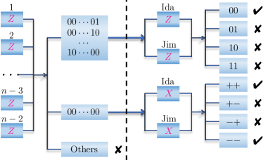
Figure 1: Schematic view of the adaptive protocol for verifying $|W_{n}\rangle$ as in Theorem 1. The dashed vertical line indicates that the protocol is two-step adaptive. For any two qubits $i$ and $j$ (Ida and Jim) chosen a priori, the measurement outcomes of the other $n-2$ qubits determine which measurements on them to perform.

It turns out that the tests based on $(YY)$ and $(ZZ)$ measurements in Eq. (6) can be dropped out if randomization is considered. The resulting protocol is illustrated in Fig. 1, and its efficiency is guaranteed by the following theorem, which is proved in Appendix B.

Theorem 1.

$|W_{n}\rangle$ can be verified efficiently using the strategy

$$\Omega_{W} = \frac{1}{C_{n}^{2}}\sum_{i<j}\Omega_{i,j}^{\rightarrow}$$ (7)

with

$$\Omega_{i,j}^{\rightarrow}=\bar{\cal Z}_{i,j}^{1}(Z_{i}^{+}Z_{j}^{+})+\bar{\cal Z}_{i,j}^{0}(XX)_{i,j}^{+}\,,$$ (8)

where the notation $\bar{\cal Z}_{i,j}^{k}$ means that $k$ excitations are detected when we perform $Z$ measurements on all qubits except for $i$ and $j$. The spectral gap is $\nu(\Omega_{W})=\frac{1}{3}$ when $n=3$ and

$$\nu(\Omega_{W})=\frac{1}{n-1}\quad\mbox{for}\,\,n\geq 4\,.$$ (9)

The test $\Omega_{i,j}^{\rightarrow}$ in Eq. (7) can be realized using adaptive measurements with two distinct measurement settings: $n-2$ parties except for parties $i$ and $j$ perform $Z$ measurements, then parties $i$ and $j$ perform either $Z$ or $X$ measurements depending on whether an excitation is detected or not in the first stage. The strategy $\Omega_{W}$ is composed of $C_{n}^{2}=\frac{1}{2}n(n-1)$ tests with probability $2/[n(n-1)]$ each. Since all these tests can be turned into each other by permuting the qubits, our protocol can be realized using only two measurement settings if permutations of qubits can be realized.

Before proceeding further, we show that Theorem 1 inspires an efficient nonadaptive protocol, although the verification efficiency would deteriorate by a factor of 2. The basic idea is to replace the adaptive test $\Omega_{i,j}^{\rightarrow}$ with two nonadaptive tests, performed with equal probability. In one test, all parties perform $Z$ measurements, and the test is passed if excitation is detected once. In the other test, parties $i$ and $j$ perform $X$ measurements, and the other $n-2$ parties perform $Z$ measurements; the test is passed if one excitation is detected for $Z$ measurements, or no excitation is detected and the outcomes for parties $i$ and $j$ coincide. The respective test projectors read

$$\mathcal{Z}^{1} =\bar{\cal Z}_{i,j}^{1}(Z_{i}^{+}Z_{j}^{+})+\bar{\cal Z}_{i,j}^{0}(ZZ)^{-}_{i,j}\,,$$ (10)

$$\Omega_{i,j} =\bar{\cal Z}_{i,j}^{0}(XX)_{i,j}^{+}+\bar{\cal Z}_{i,j}^{1}(\openone\openone)_{i,j}\,.$$ (11)

Here $\mathcal{Z}^{1}$ can also be expressed as $\mathcal{Z}^{1}=\sum_{u\in B_{n,1}}\mbox{$|u\rangle$}\mbox{$\langle u|$}$ with $B_{n,1}$ being the set of strings in $\{0,1\}^{n}$ with Hamming weight $1$. Note that $\mathcal{Z}^{1}$ is independent of $i,j$, unlike $\Omega_{ij}$. The resulting verification operator reads

$$\tilde{\Omega}_{W}=\frac{1}{2C_{n}^{2}}\sum_{i<j}\left(\mathcal{Z}^{1}+\Omega_{i,j}\right)=\frac{1}{2}\mathcal{Z}^{1}+\frac{1}{2C_{n}^{2}}\sum_{i<j}\Omega_{i,j},$$ (12)

and the spectral gap satisfies

$$\nu(\tilde{\Omega}_{W})\geq\nu\!\left(\frac{1}{2}\Omega_{W}+\frac{1}{2}\openone^{\otimes n}\right)\geq\frac{1}{2}\nu(\Omega_{W})\,.$$ (13)

This bound is actually saturated when $n\geq 4$ (see the proof in Appendix C); in the case $n=3$, direct calculation shows that $\nu(\tilde{\Omega}_{W_{3}})=\frac{3}{4}\nu(\Omega_{W_{3}})$. Hence, the verification efficiency of $\tilde{\Omega}_{W}$ is worse than that of the adaptive protocol $\Omega_{W}$ by a factor of at most 2.

When $n=3$ for example, we have

$$\Omega_{W_{3}} = \frac{1}{3}\Bigl{[}Z_{3}^{-}(Z_{2}^{+}Z_{1}^{+})+Z_{3}^{+}(XX)_{2,1}^{+}+Z_{2}^{-}(Z_{3}^{+}Z_{1}^{+})$$ (14)

$$+ Z_{2}^{+}(XX)_{3,1}^{+}+Z_{1}^{-}(Z_{3}^{+}Z_{2}^{+})+Z_{1}^{+}(XX)_{3,2}^{+}\Bigr{]}$$

for the adaptive protocol. It is easy to verify that $\lambda_{2}(\Omega_{W_{3}})=\frac{2}{3}$ and $\nu(\Omega_{W_{3}})=\frac{1}{3}$. So the number of tests required to verify $|W_{3}\rangle$ within infidelity $\epsilon$ and confidence $1-\delta$ is $N\approx 3\epsilon^{-1}\ln\delta^{-1}$. For the nonadaptive protocol $\tilde{\Omega}_{W_{3}}$, we have $\nu(\tilde{\Omega}_{W_{3}})=\frac{1}{4}$, so the number of tests required is $N\approx 4\epsilon^{-1}\ln\delta^{-1}$. These results are corroborated by numerical simulations in which we choose the worst noise in the eigenspace corresponding to the second largest eigenvalue and get $N\approx 3.0031(\pm 0.0169)\epsilon^{-1}\ln\delta^{-1}$ for the adaptive protocol and $N\approx 3.9806(\pm 0.0109)\epsilon^{-1}\ln\delta^{-1}$ for the nonadaptive one. Similarly, we get $N\approx 7.0306(\pm 0.0188)\epsilon^{-1}\ln\delta^{-1}$ (adaptive) and $N\approx 14.0621(\pm 0.0262)\epsilon^{-1}\ln\delta^{-1}$ (nonadaptive) for $|W_{8}\rangle$. More details on the simulated experiments can be found in Appendix D.

IV Verification of Dicke states

Our protocols for verifying $W$ states can be naturally generalized to arbitrary $n$-qubit Dicke states $|D_{n}^{k}\rangle$. Since $|D_{n}^{n-1}\rangle$ is equivalent to $\mbox{$|D_{n}^{1}\rangle$}=\mbox{$|W_{n}\rangle$}$ under a local unitary transformation, we can assume $2\leq k\leq n-2$ and $n\geq 4$ without loss of generality. For any pair of parties $i$ and $j$, we can construct a test as follows (see Fig. $4$ in Appendix E for an illustration). First we perform $Z$ measurements on $n-2$ parties other than parties $i$ and $j$. If the outcomes have $k$ or $k-2$ excitations, then we perform $(ZZ)$ measurements on qubits $i$ and $j$ and the test is passed if the total number of excitations is $k$; if the outcomes have $k-1$ excitations, then we perform $(XX)$ measurements and the test is passed if the two outcomes for parties $i$ and $j$ coincide. By randomizing the choice of the pair $i,j$ we can construct a verification protocol that is composed of $n(n-1)/2$ tests. The efficiency of this protocol is guaranteed by the following theorem, which is proved in Appendix E.

Theorem 2.

$|D_{n}^{k}\rangle$ can be verified efficiently using the strategy

$$\Omega_{D} = \frac{1}{C_{n}^{2}}\sum_{i<j}\Omega_{i,j}^{\rightarrow}$$ (15)

with

$$\Omega_{i,j}^{\rightarrow}=\bar{\cal Z}_{i,j}^{k}(Z_{i}^{+}Z_{j}^{+})+\bar{\cal Z}_{i,j}^{k-2}(Z_{i}^{-}Z_{j}^{-})+\bar{\cal Z}_{i,j}^{k-1}(XX)_{i,j}^{+}\,.$$ (16)

The spectral gap is

$$\nu(\Omega_{D})=\frac{1}{n-1}\quad\mbox{for}\,\,n\geq 4\,.$$ (17)

Several remarks are in order. First, when $k=1$, the second term in Eq. (16) drops out and we get back Eq. (8) as expected. Second, although we need to consider three different cases in constructing $\Omega_{i,j}^{\rightarrow}$, only two distinct measurement settings are required, which is the same as that for $W$ states. Last, the spectral gap $\nu(\Omega_{D})$ is independent of $k$ and is the same as that for $W$ states. Therefore, all $n$-qubit Dicke states can be verified using the same experimental setup and with the same efficiency. To achieve infidelity $\epsilon$ and confidence $1-\delta$, the total number of tests required is only $N\approx(n-1)\epsilon^{-1}\ln\delta^{-1}$, so our protocol is able to verify Dicke states of hundreds of qubits.

Similar to the case of $W$ states, Theorem 2 also inspires an efficient nonadaptive protocol. The basic idea is to replace the adaptive test $\Omega_{i,j}^{\rightarrow}$ with two nonadaptive tests as characterized by the two test projectors

$$\mathcal{Z}^{k}=\bar{\cal Z}_{i,j}^{k}(Z_{i}^{+}Z_{j}^{+})+\bar{\cal Z}_{i,j}^{k-2}(Z_{i}^{-}Z_{j}^{-})+\bar{\cal Z}_{i,j}^{k-1}(ZZ)^{-}_{i,j}\,,$$ (18)

$$\Omega_{i,j}=\bar{\cal Z}_{i,j}^{k-1}(XX)_{i,j}^{+}+\bar{\cal Z}_{i,j}^{k}(\openone\openone)_{i,j}+\bar{\cal Z}_{i,j}^{k-2}(\openone\openone)_{i,j}\,.$$ (19)

Here $\mathcal{Z}^{k}$ can also be expressed as $\mathcal{Z}^{k}=\sum_{u\in B_{n,k}}\mbox{$|u\rangle$}\mbox{$\langle u|$}$ with $B_{n,k}$ being the set of strings in $\{0,1\}^{n}$ with Hamming weight $k$. The resulting verification operator reads

$$\tilde{\Omega}_{D}=\frac{1}{2C_{n}^{2}}\sum_{i<j}\left(\mathcal{Z}^{k}+\Omega_{i,j}\right)=\frac{1}{2}\mathcal{Z}^{k}+\frac{1}{2C_{n}^{2}}\sum_{i<j}\Omega_{i,j},$$ (20)

and the spectral gap satisfies

$$\nu(\tilde{\Omega}_{D})\geq\nu\!\left(\frac{1}{2}\Omega_{D}+\frac{1}{2}\openone^{\otimes n}\right)\geq\frac{1}{2}\nu(\Omega_{D})\,.$$ (21)

This bound is actually saturated given the assumption $n\geq 4$ (see the proof in Appendix F). Hence, the verification efficiency of $\tilde{\Omega}_{D}$ is worse than that of the adaptive protocol $\Omega_{D}$ by a factor of 2.

Take $|D_{4}^{2}\rangle$ as an example. The second largest eigenvalue and spectral gap of $\Omega_{D_{4}^{2}}$ (see Appendix G for an explicit expression) read $\lambda_{2}(\Omega_{D_{4}^{2}})=\frac{2}{3}$ and $\nu(\Omega_{D_{4}^{2}})=\frac{1}{3}$. So the number of tests required to verify $|D_{4}^{2}\rangle$ within infidelity $\epsilon$ and confidence $1-\delta$ is $N\approx 3\epsilon^{-1}\ln\delta^{-1}$. For the nonadaptive protocol $\tilde{\Omega}_{D_{4}^{2}}$, we have $\nu(\tilde{\Omega}_{D_{4}^{2}})=\frac{1}{6}$, so the number of tests required is $N\approx 6\epsilon^{-1}\ln\delta^{-1}$. See the numerical confirmations in Appendix D.

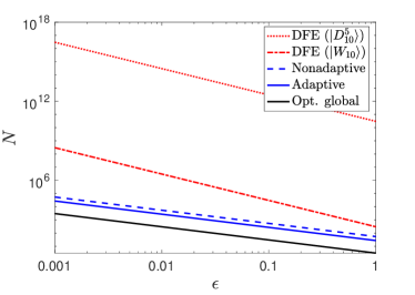
Figure 2: Comparison between our efficient adaptive and nonadaptive protocols with the DFE protocol Flammia and Liu (2011) and the optimal global protocol. For a given number of qubits $n=10$ and confidence $1-\delta=0.95$, the plot shows the number of tests $N$ required to verify $|W_{10}\rangle$ and $|D_{10}^{5}\rangle$ within infidelity $\epsilon$ for each protocol.

V Comparison with other methods

Here, we compare our adaptive and nonadaptive protocols with two other non-tomographic methods. The first one is the protocol of direct fidelity estimation (DFE) proposed in Ref. Flammia and Liu (2011). For an $n$-qubit Dicke state with $k$ excitations, this protocol requires $N\propto O(n^{2k}\epsilon^{-2}\ln\delta^{-1})$ tests, and the number of measurement settings has the same order of magnitude. This number increases exponentially with $n$ if ${k\propto n}$, which is the case for the balanced Dicke state with $k=n/2$. The second one is the optimal global verification protocol with the entangled verification operator $\Omega=\mbox{$|D_{n}^{k}\rangle$}\mbox{$\langle D_{n}^{k}|$}$, which requires $N\approx\epsilon^{-1}\ln\delta^{-1}$ tests.

In Fig. 2, by fixing the number of qubits $n=10$ and the confidence $1-\delta=0.95$, we plot the number of tests $N$ required to verify $|W_{10}\rangle$ and $|D_{10}^{5}\rangle$ within infidelity $\epsilon$. As can be seen, our adaptive and nonadaptive protocols are much more efficient than DFE and are comparable to the best protocol based on entangling measurements. In addition, similar to the optimal global protocol, the performances of our protocols are independent of the number of excitations $k$, while the performance of DFE deteriorates quickly as $k$ increases and is already impractical for $k=5$ and $\epsilon=0.1$.

VI Construction of nonadaptive protocols from adaptive protocols

Inspired by the above results, here we present a general method for converting adaptive verification protocols to nonadaptive ones at the price of efficiency. To this end, we need a notion for characterizing the complexity of an adaptive protocol. As shown in Fig. 1, an adaptive test is usually composed of a number of branches. The branch number of the test $\Omega_{j}$, denoted by $\alpha(\Omega_{j})$, is defined as the total number of such branches in realizing $\Omega_{j}$, and the branch number of a protocol is the maximum branch number over all tests. For example, the branch numbers of the adaptive protocols $\Omega_{W}$ and $\Omega_{D}$ are $2$ and $3$, respectively. To construct a nonadaptive protocol, we can replace each adaptive test with a number of nonadaptive tests depending on the branch number, which sets a lower bound for the efficiency. More precisely, we have the following theorem.

Theorem 3.

In quantum state verification, an adaptive protocol $\Omega=\sum_{j=1}^{m}\mu_{j}\Omega_{j}$ can always be converted to a nonadaptive one $\tilde{\Omega}$ whose spectral gap satisfies

$$\nu(\tilde{\Omega})\geq\frac{1}{\alpha}\nu(\Omega)\,,$$ (22)

where $\alpha=\max_{j}\{\alpha(\Omega_{j})\}$ is the branch number of the adaptive protocol $\Omega$.

Proof.

For simplicity, here we consider a two-step adaptive test of the form (but our idea is applicable in general)

$$\Omega_{j}=\sum_{a=1}^{\alpha_{j}}M_{a|j}\otimes N_{a|j}\,,$$ (23)

where $\alpha_{j}=\alpha(\Omega_{j})$, and $\{M_{a|j}\}_{a}$ represents a (possibly incomplete) generalized measurement on subsystem $A$, i.e., $M_{a|j}\geq 0$ and $\sum_{a=1}^{\alpha}M_{a|j}\leq\openone_{A}$, while $N_{a|j}$ represents a test on subsystem $B$ that depends on the outcome $a$ and satisfies $0\leq N_{a|j}\leq\openone_{B}$. Here both $A$ and $B$ may consist of one or more subsystems. Based on the adaptive test $\Omega_{j}$ we can construct $\alpha_{j}$ nonadaptive tests

$$\tilde{\Omega}_{a|j}=M_{a|j}\otimes N_{a|j}+\sum_{b\neq a}M_{b|j}\otimes\openone_{B}\,,$$ (24)

and the corresponding nonadaptive strategy is

$$\tilde{\Omega}=\sum_{j=1}^{m}\sum_{a=1}^{\alpha_{j}}\frac{\mu_{j}}{\alpha_{j}}\tilde{\Omega}_{a|j}\,,$$ (25)

which satisfies $\tilde{\Omega}\mbox{$|\psi\rangle$}=\mbox{$|\psi\rangle$}$ whenever $\Omega\mbox{$|\psi\rangle$}=\mbox{$|\psi\rangle$}$. Now, we have

$$\nu(\tilde{\Omega})=\nu\!\left(\frac{1}{\alpha}\Omega+\Omega^{\prime}\right)\geq\frac{1}{\alpha}\nu(\Omega)\,,$$ (26)

where the inequality follows from $\Omega^{\prime}=\sum_{j=1}^{m}\mu_{j}\bigl{(}1-\frac{1}{\alpha_{j}}\bigr{)}\bigl{(}\sum_{a=1}^{\alpha_{j}}M_{a|j}\bigr{)}\otimes\openone_{B}+\sum_{j=1}^{m}\mu_{j}\bigl{(}\frac{1}{\alpha_{j}}-\frac{1}{\alpha}\bigr{)}\sum_{a=1}^{\alpha_{j}}\bigl{(}M_{a|j}\otimes N_{a|j}\bigr{)}\leq\bigl{(}1-\frac{1}{\alpha}\bigr{)}\openone$. ∎

According to Theorem 3, an efficient adaptive protocol can be converted to an efficient nonadaptive one if the branch number $\alpha$ is small. This is the case for our adaptive protocols for verifying $W$ states and Dicke states, in which $\alpha$ equals $2$ and $3$, respectively. In addition, the adaptive protocols proposed in Refs. Yu et al. ; Li et al. (2019); Wang and Hayashi (2019) for general bipartite pure states can be converted to nonadaptive ones by our method. Note that in the above construction, we are interested in a general recipe; for a specific adaptive strategy, sometimes one can construct better nonadaptive strategies. For instance, if several branches happen to require the same measurement setting, we can merge these branches into one, which is the case for the verification of Dicke states.

VII Conclusions

Efficient and reliable characterization of quantum states plays a vital role in almost all quantum information processing tasks as well as foundational studies. Using both adaptive and nonadaptive approaches, here we proposed efficient and practical protocols for verifying arbitrary $n$-qubit Dicke states, including $W$ states. Both adaptive and nonadaptive protocols require only two distinct settings based on Pauli measurements together with permutations of the qubits, which is well within the reach of current experimental techniques. To verify an $n$-qubit Dicke state within infidelity $\epsilon$ and confidence $1-\delta$, both protocols require only $O(n\epsilon^{-1}\ln\delta^{-1})$ tests, which is exponentially more efficient than all previous protocols based on local measurements. Thus, our protocols are able to verify Dicke states of hundreds of qubits. Moreover, we introduced a general method for constructing nonadaptive verification protocols from adaptive protocols. Our work opens the possibility of efficiently verifying many other interesting multipartite states in the future, even the possibility of developing a general verification strategy for all states eventually.

Appendix A Verification of Bell states

Bell states can be verified optimally using the protocol in Ref. Pallister et al. (2018) (see also Refs. Hayashi et al. (2006); Hayashi ; Zhu and Hayashi (2019)). For the particular Bell state that we consider in this work, i.e., $\mbox{$|W_{2}\rangle$}=\frac{1}{\sqrt{2}}(\mbox{$|01\rangle$}+\mbox{$|10\rangle$})$, the optimal strategy reads

$$\Omega_{\mathrm{Bell}}=\frac{1}{3}\left[(XX)^{+}+(YY)^{+}+(ZZ)^{-}\right],$$ (27)

which reproduces Eq. (6) in the main text, and the spectral gap is $\nu(\Omega_{\mathrm{Bell}})=\frac{2}{3}$. To verify the Bell state within infidelity $\epsilon$ and confidence level $1-\delta$, the number of required tests is $N\approx\frac{3}{2}\epsilon^{-1}\ln\delta^{-1}$.

As an alternative, one can modify the optimal protocol by removing the test based on measurement $(YY)$ Pallister et al. (2018); Zhu and Hayashi (2019). Then the verification operator reads

$$\Omega_{W_{2}}=\frac{1}{2}\left[(XX)^{+}+(ZZ)^{-}\right],$$ (28)

and the spectral gap reduces to $\nu(\Omega_{\mathrm{Bell}})=\frac{1}{2}$. Accordingly, the number of tests increases to $N\approx 2\epsilon^{-1}\ln\delta^{-1}$. This protocol requires only two measurement settings instead of three although the efficiency is slightly worse. This observation was instrumental in constructing efficient protocols for verifying $W$ and Dicke states at the beginning of our study.

Appendix B Proof of Theorem 1

Theorem 1 is an immediate consequence of the following lemma, which provides more details on the verification operator $\Omega_{W}$.

Lemma 1.

For $n\geq 3$, the verification operator $\Omega_{W}$ has five different eigenvalues $1,1-\frac{1}{n-1},\frac{1}{2}+\frac{1}{n(n-1)},\frac{1}{n(n-1)},0$ with multiplicities $1,n-1,1,\frac{1}{2}n(n-1)-1$, and $2^{n}-\frac{1}{2}(n^{2}+n)$, respectively. When $n=3$, the second largest eigenvalue of $\Omega_{W}$ is $\lambda_{2}(\Omega_{W})=\frac{2}{3}$, which is nondegenerate, and the spectral gap is $\nu(\Omega_{W})=\frac{1}{3}$. When $n\geq 4$, the second largest eigenvalue is $\lambda_{2}(\Omega_{W})=1-\frac{1}{n-1}$ with multiplicity $n-1$, the spectral gap is $\nu(\Omega_{W})=\frac{1}{n-1}$, and the corresponding eigenspace is spanned by

$$\mbox{$|\phi_{ij}\rangle$}=\mbox{$|\psi^{-}\rangle$}_{i,j}\otimes\mbox{$|0\rangle$}^{\otimes(n-2)}\,,\quad 1\leq i<j\leq n\,.$$ (29)

where $\mbox{$|\psi^{-}\rangle$}=\frac{1}{\sqrt{2}}(\mbox{$|01\rangle$}-\mbox{$|10\rangle$})$ is the singlet.

Proof.

For $n\geq 3$, recall that $\Omega_{W}$ is defined as

$$\Omega_{W}= \frac{1}{C_{n}^{2}}\sum_{i<j}\bar{\mathcal{Z}}_{i,j}^{1}(Z_{i}^{+}Z_{j}^{+})+\frac{1}{C_{n}^{2}}\sum_{i<j}\bar{\mathcal{Z}}_{i,j}^{0}(XX)_{i,j}^{+}$$

$$= \frac{1}{C_{n}^{2}}\sum_{i<j}\bar{\mathcal{Z}}_{i,j}^{1}(Z_{i}^{+}Z_{j}^{+})+\frac{1}{C_{n}^{2}}\sum_{i<j}\bar{\mathcal{Z}}_{i,j}^{0}\otimes\bigl{(}\mbox{$|\psi^{+}\rangle$}\mbox{$\langle\psi^{+}|$}\bigr{)}_{i,j}$$

$$+\frac{1}{C_{n}^{2}}\sum_{i<j}\bar{\mathcal{Z}}_{i,j}^{0}\otimes\bigl{(}\mbox{$|\varphi^{+}\rangle$}\mbox{$\langle\varphi^{+}|$}\bigr{)}_{i,j}\,,$$ (30)

where $\mbox{$|\psi^{+}\rangle$}=\frac{1}{\sqrt{2}}(\mbox{$|01\rangle$}+\mbox{$|10\rangle$})$ and $\mbox{$|\varphi^{+}\rangle$}=\frac{1}{\sqrt{2}}(\mbox{$|00\rangle$}+\mbox{$|11\rangle$})$ are Bell states. Direct calculations show that

$$\frac{1}{C_{n}^{2}}\sum_{i<j}\bar{\mathcal{Z}}_{i,j}^{1}(Z_{i}^{+}Z_{j}^{+})=\frac{n-2}{n}\mathcal{Z}^{1}\,,$$ (31)

$$\frac{1}{C_{n}^{2}}\sum_{i<j}\bar{\mathcal{Z}}_{i,j}^{0}\otimes\bigl{(}\mbox{$|\psi^{+}\rangle$}\mbox{$\langle\psi^{+}|$}\bigr{)}_{i,j}=\frac{1}{2C_{n}^{2}}\Big{[}n\mbox{$|W_{n}\rangle$}\mbox{$\langle W_{n}|$}+(n-2)\mathcal{Z}^{1}\Big{]},$$ (32)

$$\frac{1}{C_{n}^{2}}\sum_{i<j}\bar{\mathcal{Z}}_{i,j}^{0}\otimes\bigl{(}\mbox{$|\varphi^{+}\rangle$}\mbox{$\langle\varphi^{+}|$}\bigr{)}_{i,j}=\frac{1}{2C_{n}^{2}}\Big{[}C_{n}^{2}\mbox{$|\phi_{0}\rangle$}\mbox{$\langle\phi_{0}|$}+\left(\mathcal{Z}^{0}+\mathcal{Z}^{2}-\mbox{$|\phi_{1}\rangle$}\mbox{$\langle\phi_{1}|$}\right)\!\Big{]},$$ (33)

where

$$|\phi_{0}\rangle =\,\,{\cal N}\!\left[\sqrt{C_{n}^{2}}\mbox{$|D_{n}^{0}\rangle$}+\mbox{$|D_{n}^{2}\rangle$}\right]\!,$$ (34)

$$|\phi_{1}\rangle =\,\,{\cal N}\!\left[\mbox{$|D_{n}^{0}\rangle$}-\sqrt{C_{n}^{2}}\mbox{$|D_{n}^{2}\rangle$}\right]\!,$$ (35)

with ${\cal N}[\cdot]$ denoting the normalization of the vector inside. Note that $|W_{n}\rangle$ belongs to the support of $\mathcal{Z}^{1}$, while $|\phi_{0}\rangle$ and $|\phi_{1}\rangle$ belong to the support of $\mathcal{Z}^{0}+\mathcal{Z}^{2}$ and satisfy $\mbox{$\langle\phi_{0}|\phi_{1}\rangle$}=0$. Therefore, $\Omega_{W}$ has five different eigenvalues $1,1-\frac{1}{n-1},\frac{1}{2}+\frac{1}{n(n-1)},\frac{1}{n(n-1)},0$ with multiplicities 1, $n-1$, 1, $\frac{1}{2}n(n-1)-1$, and $2^{n}-\frac{1}{2}(n^{2}+n)$, respectively. The second largest eigenvalue of $\Omega_{W}$ is achieved either in the support of $\mathcal{Z}^{1}-\mbox{$|W_{n}\rangle$}\mbox{$\langle W_{n}|$}$ or in the eigenvector $|\phi_{0}\rangle$, that is,

$$\lambda_{2}(\Omega_{W})=\max\left\{1-\frac{1}{n-1},\frac{1}{2}+\frac{1}{n(n-1)}\right\}\!,$$ (36)

for all $n\geq 3$. Accordingly, the spectral gap from the largest eigenvalue reads

$$\nu(\Omega_{W})=\min\left\{\frac{1}{n-1},\frac{1}{2}-\frac{1}{n(n-1)}\right\}\!,$$ (37)

for all $n\geq 3$. It is easy to see that $\lambda_{2}(\Omega_{W})=\frac{2}{3}$ and $\nu(\Omega_{W})=\frac{1}{3}$ when $n=3$, and the corresponding eigenvector is $|\phi_{0}\rangle$ in Eq. (34). When $n\geq 4$, we have $\lambda_{2}(\Omega_{W})=1-\frac{1}{n-1}$, $\nu(\Omega_{W})=\frac{1}{n-1}$, and the corresponding eigenspace coincides with the support of $\mathcal{Z}^{1}-\mbox{$|W_{n}\rangle$}\mbox{$\langle W_{n}|$}$, which is an $(n-1)$-dimensional subspace spanned by the kets $|\phi_{ij}\rangle$ in Eq. (29). ∎

To briefly summarize, Theorem 1 provides an efficient verification protocol for any $n$-qubit $W$ state $|W_{n}\rangle$. In real experiments, the experimenter needs to perform the following procedure in each run of the verification protocol:

• The $n$ parties use shared randomness or classical communication to randomly choose any two parties, e.g., $i$ and $j$ (Ida and Jim).

• All the rest $n-2$ parties perform Pauli-$Z$ measurements, then send their outcomes to Ida and Jim.

  • If the outcome $1$ does not appear for all the $n-2$ Pauli-$Z$ measurements, then both Ida and Jim perform Pauli-$X$ measurements.

    • If the two Pauli-$X$ measurements give the same outcome, then they announce the result “pass”; otherwise they announce the result “fail”.

  • If the outcome $1$ appears exactly once for the $n-2$ Pauli-$Z$ measurements, then both Ida and Jim perform Pauli-$Z$ measurements.

    • If both of them obtain outcome $0$, then they announce the result “pass”; otherwise, they announce the result “fail”.

  • If the outcome $1$ appears more than once for the $n-2$ Pauli-$Z$ measurements, then Ida and Jim announce the result “fail”.

Appendix C Proof of the saturation of the bound in Eq. (13)

In this appendix, we prove the saturation of the bound in Eq. (13) when $n\geq 4$. In the case $n=3$, direct calculation shows that $\nu(\tilde{\Omega}_{W_{3}})=\frac{3}{4}\nu(\Omega_{W_{3}})$. See below the lemma.

Lemma 2.

When $n\geq 4$, $\nu(\tilde{\Omega}_{W})=\frac{1}{2}\nu(\Omega_{W})$.

Proof.

In the main text, we have already proved that $\nu(\tilde{\Omega}_{W})\geq\frac{1}{2}\nu(\Omega_{W})$. Hence, to prove the saturation of the bound, we just need to show that $\nu(\tilde{\Omega}_{W})\leq\frac{1}{2}\nu(\Omega_{W})$. Be reminded that $\nu(\tilde{\Omega}_{W})$ can be written as

$$\nu(\tilde{\Omega}_{W}):=1-\max_{\mbox{$\langle\phi|W_{n}\rangle$}=0}\mbox{$\langle\phi|$}\tilde{\Omega}_{W}\mbox{$|\phi\rangle$}\,.$$ (38)

By taking $|\phi\rangle$ to be $|\phi_{ij}\rangle$ defined in Eq. (29), which are orthogonal to $|W_{n}\rangle$, we get an upper bound of $\nu(\tilde{\Omega}_{W})$, i.e.,

$$\nu(\tilde{\Omega}_{W})\leq 1-\mbox{$\langle\phi_{ij}|$}\tilde{\Omega}_{W}\mbox{$|\phi_{ij}\rangle$}=\frac{1}{2(n-1)}=\frac{1}{2}\nu(\Omega_{W})\,.$$ (39)

This inequality completes the proof. ∎

Appendix D Simulated experiments on quantum state verification

Here we show how to perform simulated experiments on quantum state verification (QSV). As a demonstration, we use the verification protocols for $W$ states and Dicke states as characterized by the operators $\Omega_{W/D}=\frac{1}{C_{n}^{2}}\sum_{i<j}\Omega_{i,j}^{\rightarrow}$.

To set the input state, we add noise to the target state $|\psi\rangle$ such that

$$\mbox{$|\psi^{\prime}\rangle$}=\sqrt{1-\epsilon}\mbox{$|\psi\rangle$}+\sqrt{\epsilon}\mbox{$|\tau\rangle$}\,,$$ (40)

where the noisy state $|\tau\rangle$ is chosen in the vector space corresponding to the second largest eigenvalue of $\Omega_{W/D}$. Other kinds of noise, including random noise, would be easier to detect. Then, for each input state $|\psi^{\prime}\rangle$, we perform one of the $C_{n}^{2}$ tests $\Omega_{i,j}^{\rightarrow}$ randomly with probability $1/{C_{n}^{2}}$ each. If $|\psi^{\prime}\rangle$ passes the test (with probability $\mathrm{tr}(\Omega_{i,j}^{\rightarrow}\mbox{$|\psi^{\prime}\rangle$}\mbox{$\langle\psi^{\prime}|$})$), we continue with the next one. Otherwise, the verification protocol ends and we record the number of “pass” instances. This process is repeated many times, from which we calculate the minimum number of tests required to achieve a given confidence level $1-\delta$. Specifically, the simulation procedure can be formulated as in the following algorithm.

Algorithm ​​: Simulated experiments on QSV

1:Input: The target state $|\psi\rangle$, the noise $|\tau\rangle$, the infidelity $\epsilon$, and the confidence level $1-\delta$.

2:Objective: Determine the number of tests $N$ required to verify $|\psi\rangle$ within infidelity $\epsilon$ and confidence $1-\delta$.

3:Init: Set the input state $|\psi^{\prime}\rangle$ as in Eq. (40).

4:Measure: Perform one of the $C_{n}^{2}$ tests $\Omega_{i,j}^{\rightarrow}$ on $|\psi^{\prime}\rangle$ randomly with probability $1/{C_{n}^{2}}$ each.

5:Count: If $|\psi^{\prime}\rangle$ passes the test, then repeat step 2. Otherwise, end the verification procedure and record the number of “pass” instances $N_{i}$.

6:Loop: Repeat steps 2 and 3 above $M$ times and record the $M$ numbers $N_{i}$ for $i=1,2,\ldots,M$.

7:Output: Arrange $N_{i}$ in decreasing order and then output $N:=N_{\lfloor\delta M\rfloor}$.

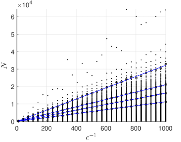
Figure 3: Simulation results on the adaptive verification of $|W_{8}\rangle$. The two axes denote the number of tests $N$ and the reciprocal of the infidelity $\epsilon^{-1}$. For each $\epsilon$, the simulation is repeated $M=10000$ times, but only 500 points are shown in the plot for clarity. The open circles denote the minimum number of tests required to achieve infidelity $\epsilon$ and confidence $1-\delta$, and the four blue lines are fitted for $\delta=0.01,0.05,0.1,0.2$ (top-down), respectively. Here the number of tests can be approximated by the formula $N\approx 7.0306(\pm 0.0188)\epsilon^{-1}\ln\delta^{-1}$, which is very close to the theoretical prediction.

Table 1: Simulation results on the verification of $W$ and Dicke states. For each state, the verification procedure is repeated $M=10000$ times for both the adaptive and nonadaptive protocols. The table shows the fitted values of the parameter $\frac{1}{\nu(\Omega)}$ featuring in the formula $N\approx\frac{1}{\nu(\Omega)}\epsilon^{-1}\ln\delta^{-1}$. The values inside the parentheses are the standard deviations calculated from 100 different instances of $\delta$ taken uniformly from the interval $0.01$ to $0.2$.

State	Adaptive	Nonadaptive
$|W_{3}\rangle$	$3.0031(\pm 0.0169)$	$3.9806(\pm 0.0109)$
$|W_{4}\rangle$	$3.0088(\pm 0.0066)$	$6.0640(\pm 0.0362)$
$|W_{5}\rangle$	$3.9847(\pm 0.0076)$	$7.9825(\pm 0.0379)$
$|W_{6}\rangle$	$4.9916(\pm 0.0186)$	$9.9982(\pm 0.0310)$
$|W_{7}\rangle$	$5.9984(\pm 0.0149)$	$11.9445(\pm 0.0495)$
$|W_{8}\rangle$	$7.0306(\pm 0.0188)$	$14.0621(\pm 0.0262)$
$|D_{4}^{2}\rangle$	$2.9931(\pm 0.0058)$	$5.9411(\pm 0.0181)$
$|D_{5}^{2}\rangle$	$4.0064(\pm 0.0193)$	$7.9722(\pm 0.0245)$
$|D_{6}^{2}\rangle$	$4.9981(\pm 0.0110)$	$10.0371(\pm 0.0233)$
$|D_{6}^{3}\rangle$	$4.9654(\pm 0.0148)$	$10.0147(\pm 0.0173)$
$|D_{7}^{2}\rangle$	$6.0131(\pm 0.0118)$	$11.9302(\pm 0.0240)$
$|D_{7}^{3}\rangle$	$5.9610(\pm 0.0111)$	$11.9553(\pm 0.0366)$
$|D_{8}^{2}\rangle$	$6.9554(\pm 0.0378)$	$14.0045(\pm 0.0345)$
$|D_{8}^{4}\rangle$	$6.9554(\pm 0.0361)$	$14.0669(\pm 0.0289)$

As an example, the simulation results on the verification of $|W_{8}\rangle$ using the adaptive protocol are shown in Fig. 3. By numerical fitting we get the approximation $\frac{1}{\nu(\Omega)}\approx 7.0306(\pm 0.0188)$, which is very close to the theoretical value of 7. For more simulation results, see Table 1.

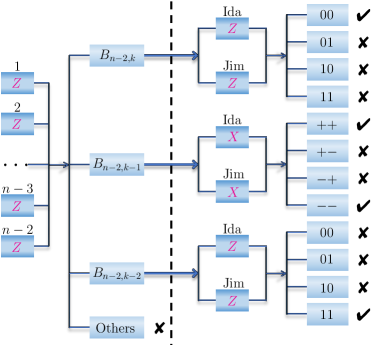
Figure 4: Schematic view of the adaptive protocol for verifying the Dicke state $|D_{n}^{k}\rangle$ as in Theorem 2. The protocol is two-step adaptive as indicated by the dashed vertical line. For any two qubits $i$ and $j$ (Ida and Jim) chosen a priori, the outcomes of $Z$ measurements on the other $n-2$ qubits determine which measurements on them to perform. Recall that $B_{n,k}$ denotes the set of all strings in $\{0,1\}^{n}$ that have Hamming weight $k$, where 0 and 1 correspond to eigenvalues 1 and $-1$ of $Z$, respectively.

Appendix E Proof of Theorem 2

In this Appendix, we prove Theorem 2 and give more details on the adaptive verification protocol for Dicke states. First, see Fig. 4 for a schematic view of this verification protocol. Theorem 2 is a consequence of the following lemma, which is a generalization of Lemma 1.

Lemma 3.

For $n\geq 4$, the second largest eigenvalue of $\Omega_{D}$ in Eq. (15) is $\lambda_{2}(\Omega_{D})=1-\frac{1}{n-1}$ with multiplicity $n-1$, and the corresponding eigenspace is spanned by

$$\mbox{$|\phi_{ij}\rangle$}=\mbox{$|\psi^{-}\rangle$}_{i,j}\otimes\mbox{$|D_{n-2}^{k-1}\rangle$}\,,\quad 1\leq i<j\leq n\,,$$ (41)

where $\mbox{$|\psi^{-}\rangle$}=\frac{1}{\sqrt{2}}(\mbox{$|01\rangle$}-\mbox{$|10\rangle$})$ is the singlet.

Proof.

When $k=1$ or $k=n-1$, the conclusion follows from Lemma 1, so here we can assume $2\leq k\leq n-2$. Recall that $\Omega_{D}$ is defined as

$$\Omega_{D}= \frac{1}{C_{n}^{2}}\sum_{i<j}\big{[}\bar{\mathcal{Z}}_{i,j}^{k}(Z_{i}^{+}Z_{j}^{+})+\bar{\mathcal{Z}}_{i,j}^{k-2}(Z_{i}^{-}Z_{j}^{-})\big{]}+\frac{1}{C_{n}^{2}}\sum_{i<j}\bar{\mathcal{Z}}_{i,j}^{k-1}(XX)_{i,j}^{+}$$

$$= \frac{C_{n-2}^{k}+C_{n-2}^{k-2}}{C_{n}^{k}}\mathcal{Z}^{k}+\frac{1}{C_{n}^{2}}\sum_{i<j}\bar{\mathcal{Z}}_{i,j}^{k-1}\otimes\bigl{(}\mbox{$|\psi^{+}\rangle$}\mbox{$\langle\psi^{+}|$}\bigr{)}_{i,j}+\frac{1}{C_{n}^{2}}\sum_{i<j}\bar{\mathcal{Z}}_{i,j}^{k-1}\otimes\bigl{(}\mbox{$|\varphi^{+}\rangle$}\mbox{$\langle\varphi^{+}|$}\bigr{)}_{i,j}$$

$$= \frac{1}{n(n-1)}\big{(}M_{1}+M_{2}\big{)}\,,$$ (42)

where

$$M_{1}= \big{[}n(n-1)-k(n-k)\big{]}\mathcal{Z}^{k}+\sum_{\begin{subarray}{c}u,v\in B_{n,k}\\ u-v\in B_{n,2}\end{subarray}}\mbox{$|u\rangle$}\mbox{$\langle v|$}=\big{[}n(n-1)-k(n-k)\big{]}\mathcal{Z}^{k}+\sum_{u,v\in B_{n,k}}A_{uv}\mbox{$|u\rangle$}\mbox{$\langle v|$}\,,$$ (43)

$$M_{2}= \frac{(n-k)(n-k+1)}{2}\sum_{u\in B_{n,k-1}}\mbox{$|u\rangle$}\mbox{$\langle u|$}+\frac{k(k+1)}{2}\sum_{v\in B_{n,k+1}}\mbox{$|v\rangle$}\mbox{$\langle v|$}+\sum_{\begin{subarray}{c}u\in B_{n,k-1}\\ v\in B_{n,k+1}\\ u-v\in B_{n,2}\end{subarray}}\big{(}\mbox{$|u\rangle$}\mbox{$\langle v|$}+\mbox{$|v\rangle$}\mbox{$\langle u|$}\big{)}\,,$$ (44)

and $\mbox{$|\psi^{+}\rangle$}=\frac{1}{\sqrt{2}}(\mbox{$|01\rangle$}+\mbox{$|10\rangle$})$ and $\mbox{$|\varphi^{+}\rangle$}=\frac{1}{\sqrt{2}}(\mbox{$|00\rangle$}+\mbox{$|11\rangle$})$ are Bell states. Here $B_{n,k}$ denotes the set of all strings in $\{0,1\}^{n}$ that have Hamming weight $k$, and the bitwise operation $u-v$ is modulo 2; the coefficient matrix $(A_{uv})$ for $u,v\in B_{n,k}$ happens to be the adjacency matrix of the Johnson graph $J(n,k)$ Brouwer et al. (1989). Note that $M_{1}$ and $M_{2}$ are hermitian and have orthogonal supports, so both of them are positive semidefinite given that $\Omega_{D}$ is positive semidefinite by construction.

According to Theorem 9.1.2 in Ref. Brouwer et al. (1989), the distinct eigenvalues of $A$ and corresponding multiplicities read

$$(k-j)(n-k-j)-j,\quad C_{n}^{j}-C_{n}^{j-1},$$ (45)

for all $j=0,1,\ldots,\min\{k,n-k\}$, where it is understood that $C_{n}^{-1}=0$. Therefore, the two largest eigenvalues of $M_{1}$ read

$$\lambda_{1}(M_{1}) =n(n-1)\,,$$ (46)

$$\lambda_{2}(M_{1}) =n(n-1)-n=n(n-2)\,,$$

which have multiplicities 1 and $n-1$, respectively.

Now, we consider $M_{2}$. Direct calculations show that $M_{2}$ has an eigenvector

$$\mbox{$|\phi\rangle$}={\cal N}\!\left[\sqrt{C_{n}^{k+1}}\mbox{$|D_{n}^{k-1}\rangle$}+\sqrt{C_{n}^{k-1}}\mbox{$|D_{n}^{k+1}\rangle$}\right]\!.$$ (47)

As $M_{2}$ is irreducible in the subspace spanned by $|u\rangle$ with $u\in B_{n,k-1}$ or $u\in B_{n,k+1}$, i.e., the graph corresponding to the third term of $M_{2}$ in Eq. (44) is connected, Perron-Frobenius theorem (see e.g., Chapter 8 in Ref. Meyer (2000)) implies that the eigenvalue corresponding to the ket in Eq. (47) is the largest (and nondegenerate) eigenvalue of $M_{2}$, which reads

$$\lambda_{1}(M_{2})=\frac{1}{2}n(n+1)+k(k-n)\,.$$ (48)

In conjunction with Eqs. (E) and (46), we can deduce the second largest eigenvalue and its spectral gap from the largest eigenvalue,

$$\lambda_{2}(\Omega_{D})=\max\left\{1-\frac{1}{n-1},\frac{1}{2}+\frac{k(k-n)+n}{n(n-1)}\right\}\!,$$ (49)

$$\nu(\Omega_{D})=\min\left\{\frac{1}{n-1},\frac{1}{2}-\frac{k(k-n)+n}{n(n-1)}\right\}\!.$$ (50)

The above equations can be simplified by virtue of the assumption $n\geq 4$, with the result

$$\lambda_{2}(\Omega_{D}) =1-\frac{1}{n-1}\,,$$ (51)

$$\nu(\Omega_{D}) =\frac{1}{n-1}\,;$$ (52)

in addition, the second largest eigenvalue has multiplicity $n-1$. Furthermore, it is straightforward to verify that the kets $|\phi_{ij}\rangle$ in Eq. (41) are eigenvectors of $\Omega_{D}$ with eigenvalue $1-\frac{1}{n-1}$. The span of all $|\phi_{ij}\rangle$ for $1\leq i<j\leq n$ has dimension $n-1$, which accounts for the multiplicity $n-1$ of the second largest eigenvalue. ∎

To briefly summarize, Theorem 2 provides an efficient verification protocol for any Dicke state $|D_{n}^{k}\rangle$. In real experiments, the experimenter performs the following procedure in each run of the verification protocol:

• The $n$ parties use shared randomness or classical communication to randomly choose two parties, e.g., $i$ and $j$ (Ida and Jim).

• All the rest $n-2$ parties perform Pauli-$Z$ measurements, then send their outcomes to Ida and Jim.

  • If the outcome $1$ appears $k$ or $k-2$ times for the $n-2$ Pauli-$Z$ measurements, then Ida and Jim also perform Pauli-$Z$ measurements.

    • If exactly $k$ of the $n$ Pauli-$Z$ measurements give outcome $1$, then they announce the result “pass”; otherwise, they announce the result “fail”.

  • If the outcome $1$ appears $k-1$ times for the $n-2$ Pauli-$Z$ measurements, then Ida and Jim perform Pauli-$X$ measurements.

    • If the two Pauli-$X$ measurements give the same outcome, then they announce the result “pass”; otherwise, they announce the result “fail”.

  • If the outcome $1$ appears less than $k-2$ or more than $k$ times for the $n-2$ Pauli-$Z$ measurements, then Ida and Jim announce the result “fail”.

Appendix F Proof of the saturation of the bound in Eq. (21)

Similar to the case of $W$ states, we can prove the saturation of the bound in Eq. (21) when $n\geq 4$, as shown in the following lemma.

Lemma 4.

When $n\geq 4$, $\nu(\tilde{\Omega}_{D})=\frac{1}{2}\nu(\Omega_{D})$.

Proof.

In the main text, we have already proved that $\nu(\tilde{\Omega}_{D})\geq\frac{1}{2}\nu(\Omega_{D})$. Hence, to prove the saturation of the bound, we just need to show that $\nu(\tilde{\Omega}_{D})\leq\frac{1}{2}\nu(\Omega_{D})$. Note that $\nu(\tilde{\Omega}_{D})$ can be written as

$$\nu(\tilde{\Omega}_{D}):=1-\max_{\mbox{$\langle\phi|D_{n}^{k}\rangle$}=0}\mbox{$\langle\phi|$}\tilde{\Omega}_{D}\mbox{$|\phi\rangle$}\,.$$ (53)

By taking $|\phi\rangle$ to be $|\phi_{ij}\rangle$ defined in Eq. (41), which are orthogonal to $|D_{n}^{k}\rangle$, we get an upper bound of $\nu(\tilde{\Omega}_{D})$, i.e.,

$$\nu(\tilde{\Omega}_{D})\leq 1-\mbox{$\langle\phi_{ij}|$}\tilde{\Omega}_{D}\mbox{$|\phi_{ij}\rangle$}=\frac{1}{2(n-1)}=\frac{1}{2}\nu(\Omega_{D})\,,$$ (54)

which confirms the lemma. ∎

Appendix G Adaptive verification of the Dicke state $|D_{4}^{2}\rangle$

The state $|D_{4}^{2}\rangle$ has $k=2$ excitations, and the verification operator $\Omega_{D_{4}^{2}}$ of the adaptive protocol in Theorem 2 takes on the form

$$\Omega_{D_{4}^{2}}=\frac{1}{6}\Bigl{[} Z_{4}^{-}Z_{3}^{+}(XX)_{2,1}^{+}+Z_{4}^{+}Z_{3}^{-}(XX)_{2,1}^{+}+Z_{4}^{-}Z_{3}^{-}Z_{2}^{+}Z_{1}^{+}+Z_{4}^{+}Z_{3}^{+}Z_{2}^{-}Z_{1}^{-}$$

$$+ Z_{4}^{-}Z_{2}^{+}(XX)_{3,1}^{+}+Z_{4}^{+}Z_{2}^{-}(XX)_{3,1}^{+}+Z_{4}^{-}Z_{2}^{-}Z_{3}^{+}Z_{1}^{+}+Z_{4}^{+}Z_{2}^{+}Z_{3}^{-}Z_{1}^{-}$$

$$+ Z_{3}^{-}Z_{2}^{+}(XX)_{4,1}^{+}+Z_{3}^{+}Z_{2}^{-}(XX)_{4,1}^{+}+Z_{3}^{-}Z_{2}^{-}Z_{4}^{+}Z_{1}^{+}+Z_{3}^{+}Z_{2}^{+}Z_{4}^{-}Z_{1}^{-}$$

$$+ Z_{4}^{-}Z_{1}^{+}(XX)_{3,2}^{+}+Z_{4}^{+}Z_{1}^{-}(XX)_{3,2}^{+}+Z_{4}^{-}Z_{1}^{-}Z_{3}^{+}Z_{2}^{+}+Z_{4}^{+}Z_{1}^{+}Z_{3}^{-}Z_{2}^{-}$$

$$+ Z_{3}^{-}Z_{1}^{+}(XX)_{4,2}^{+}+Z_{3}^{+}Z_{1}^{-}(XX)_{4,2}^{+}+Z_{3}^{-}Z_{1}^{-}Z_{4}^{+}Z_{2}^{+}+Z_{3}^{+}Z_{1}^{+}Z_{4}^{-}Z_{2}^{-}$$

$$+ Z_{2}^{-}Z_{1}^{+}(XX)_{4,3}^{+}+Z_{2}^{+}Z_{1}^{-}(XX)_{4,3}^{+}+Z_{2}^{-}Z_{1}^{-}Z_{4}^{+}Z_{3}^{+}+Z_{2}^{+}Z_{1}^{+}Z_{4}^{-}Z_{3}^{-}\Bigr{]}.$$ (55)

The second largest eigenvalue of $\Omega_{D_{4}^{2}}$ is $\lambda_{2}(\Omega_{D_{4}^{2}})=\frac{2}{3}$, and the spectral gap is $\nu(\Omega_{D_{4}^{2}})=\frac{1}{3}$. Therefore, the number of tests required to verify $|D_{4}^{2}\rangle$ within infidelity $\epsilon$ and confidence $1-\delta$ is $N\approx 3\epsilon^{-1}\ln\delta^{-1}$. Simulation results on the verification of $|D_{4}^{2}\rangle$ can be found in Appendix C.

References

- Paris and Řeháček (2004) M. Paris and J. Řeháček, eds., Quantum State Estimation, Lecture Notes in Physics, Vol. 649 (Springer, Heidelberg, 2004).
- Häffner et al. (2005) H. Häffner, W. Hänsel, C. F. Roos, J. Benhelm, D. Chek-al-kar, M. Chwalla, T. Körber, U. D. Rapol, M. Riebe, P. O. Schmidt, C. Becher, O. Gühne, W. Dür, and R. Blatt, “Scalable multiparticle entanglement of trapped ions,” Nature 438, 643 (2005).
- Shang et al. (2017) J. Shang, Z. Zhang, and H. K. Ng, “Superfast maximum-likelihood reconstruction for quantum tomography,” Phys. Rev. A 95, 062336 (2017).
- Tóth and Gühne (2005) G. Tóth and O. Gühne, “Detecting genuine multipartite entanglement with two local measurements,” Phys. Rev. Lett. 94, 060501 (2005).
- Gühne and Tóth (2009) O. Gühne and G. Tóth, “Entanglement detection,” Phys. Rep. 474, 1 (2009).
- Dimić and Dakić (2018) A. Dimić and B. Dakić, “Single-copy entanglement detection,” npj Quantum Inf. 4, 11 (2018).
- (7) V. Saggio, A. Dimić, C. Greganti, L. A. Rozema, P. Walther, and B. Dakić, “Experimental few-copy multi-particle entanglement detection,” arXiv:1809.05455 .
- Flammia and Liu (2011) S. T. Flammia and Y.-K. Liu, “Direct fidelity estimation from few Pauli measurements,” Phys. Rev. Lett. 106, 230501 (2011).
- Mayers and Yao (2004) D. Mayers and A. Yao, “Self testing quantum apparatus,” Quantum Inf. Comput. 4, 273 (2004).
- Coladangelo et al. (2017) A. Coladangelo, K. T. Goh, and V. Scarani, “All pure bipartite entangled states can be self-tested,” Nat. Commun. 8, 15485 (2017).
- Morimae et al. (2017) T. Morimae, Y. Takeuchi, and M. Hayashi, “Verification of hypergraph states,” Phys. Rev. A 96, 062321 (2017).
- Pallister et al. (2018) S. Pallister, N. Linden, and A. Montanaro, “Optimal verification of entangled states with local measurements,” Phys. Rev. Lett. 120, 170502 (2018).
- Takeuchi and Morimae (2018) Y. Takeuchi and T. Morimae, “Verification of many-qubit states,” Phys. Rev. X 8, 021060 (2018).
- (14) H. Zhu and M. Hayashi, “Efficient verification of hypergraph states,” arXiv:1806.05565 .
- (15) X.-D. Yu, J. Shang, and O. Gühne, “Optimal verification of general bipartite pure states,” arXiv:1901.09856 .
- Li et al. (2019) Z. Li, Y.-G. Han, and H. Zhu, “Efficient verification of bipartite pure states,” Phys. Rev. A 100, 032316 (2019).
- Wang and Hayashi (2019) K. Wang and M. Hayashi, “Optimal verification of two-qubit pure states,” Phys. Rev. A 100, 032315 (2019).
- Zhu and Hayashi (2019) H. Zhu and M. Hayashi, “Optimal verification and fidelity estimation of maximally entangled states,” Phys. Rev. A 99, 052346 (2019).
- (19) H. Zhu and M. Hayashi, “General framework for verifying pure quantum states in the adversarial scenario,” arXiv:1909.01943 .
- (20) W.-H. Zhang, Z. Chen, X.-X. Peng, X.-Y. Xu, P. Yin, X.-J. Ye, J.-S. Xu, G. Chen, C.-F. Li, and G.-C. Guo, “Experimental optimal verification of entangled states using local measurements,” arXiv:1905.12175 .
- Dicke (1954) R. H. Dicke, “Coherence in spontaneous radiation processes,” Phys. Rev. 93, 99 (1954).
- Briegel and Raussendorf (2001) H. J. Briegel and R. Raussendorf, “Persistent entanglement in arrays of interacting particles,” Phys. Rev. Lett. 86, 910 (2001).
- Gühne et al. (2008) O. Gühne, F. Bodoky, and M. Blaauboer, “Multiparticle entanglement under the influence of decoherence,” Phys. Rev. A 78, 060301(R) (2008).
- Bourennane et al. (2006) M. Bourennane, M. Eibl, S. Gaertner, N. Kiesel, C. Kurtsiefer, and H. Weinfurter, “Entanglement persistency of multiphoton entangled states,” Phys. Rev. Lett. 96, 100502 (2006).
- Kiesel et al. (2007) N. Kiesel, C. Schmid, G. Tóth, E. Solano, and H. Weinfurter, “Experimental observation of four-photon entangled Dicke state with high fidelity,” Phys. Rev. Lett. 98, 063604 (2007).
- Murao et al. (1999) M. Murao, D. Jonathan, M. B. Plenio, and V. Vedral, “Quantum telecloning and multiparticle entanglement,” Phys. Rev. A 59, 156 (1999).
- Prevedel et al. (2009) R. Prevedel, G. Cronenberg, M. S. Tame, M. Paternostro, P. Walther, M. S. Kim, and A. Zeilinger, “Experimental realization of Dicke states of up to six qubits for multiparty quantum networking,” Phys. Rev. Lett. 103, 020503 (2009).
- Wieczorek et al. (2009) W. Wieczorek, R. Krischek, N. Kiesel, P. Michelberger, G. Tóth, and H. Weinfurter, “Experimental entanglement of a six-photon symmetric Dicke state,” Phys. Rev. Lett. 103, 020504 (2009).
- Pezzè et al. (2018) L. Pezzè, A. Smerzi, M. K. Oberthaler, R. Schmied, and P. Treutlein, “Quantum metrology with nonclassical states of atomic ensembles,” Rev. Mod. Phys. 90, 035005 (2018).
- Zou et al. (2018) Y.-Q. Zou, L.-N. Wu, Q. Liu, X.-Y. Luo, S.-F. Guo, J.-H. Cao, M. K. Tey, and L. You, “Beating the classical precision limit with spin-1 Dicke states of more than 10,000 atoms,” Proc. Natl. Acad. Sci. 115, 6381 (2018).
- Tóth et al. (2010) G. Tóth, W. Wieczorek, D. Gross, R. Krischek, C. Schwemmer, and H. Weinfurter, “Permutationally invariant quantum tomography,” Phys. Rev. Lett. 105, 250403 (2010).
- Moroder et al. (2012) T. Moroder, P. Hyllus, G. Tóth, C. Schwemmer, A. Niggebaum, S. Gaile, O. Gühne, and H. Weinfurter, “Permutationally invariant state reconstruction,” New J. Phys. 14, 105001 (2012).
- Gühne et al. (2007) O. Gühne, C.-Y. Lu, W.-B. Gao, and J.-W. Pan, “Toolbox for entanglement detection and fidelity estimation,” Phys. Rev. A 76, 030305(R) (2007).
- Tóth (2007) G. Tóth, “Detection of multipartite entanglement in the vicinity of symmetric Dicke states,” J. Opt. Soc. Am. B 24, 275 (2007).
- Tóth et al. (2009) G. Tóth, W. Wieczorek, R. Krischek, N. Kiesel, P. Michelberger, and H. Weinfurter, “Practical methods for witnessing genuine multi-qubit entanglement in the vicinity of symmetric states,” New J. Phys. 11, 083002 (2009).
- Huber et al. (2011) M. Huber, P. Erker, H. Schimpf, A. Gabriel, and B. Hiesmayr, “Experimentally feasible set of criteria detecting genuine multipartite entanglement in -qubit Dicke states and in higher-dimensional systems,” Phys. Rev. A 83, 040301(R) (2011).
- Novo et al. (2013) L. Novo, T. Moroder, and O. Gühne, “Genuine multiparticle entanglement of permutationally invariant states,” Phys. Rev. A 88, 012305 (2013).
- Bergmann and Gühne (2013) M. Bergmann and O. Gühne, “Entanglement criteria for Dicke states,” J. Phys. A: Math. Theor. 46, 385304 (2013).
- Šupić et al. (2018) I. Šupić, A. Coladangelo, R. Augusiak, and A. Acín, “Self-testing multipartite entangled states through projections onto two systems,” New J. Phys. 20, 083041 (2018).
- (40) M. Fadel, “Self-testing Dicke states,” arXiv:1707.01215 .
- Hayashi et al. (2006) M. Hayashi, K. Matsumoto, and Y. Tsuda, “A study of LOCC-detection of a maximally entangled state using hypothesis testing,” J. Phys. A: Math. Gen. 39, 14427 (2006).
- (42) M. Hayashi, “Discrete realization of group symmetric LOCC-detection of maximally entangled state,” arXiv:0810.3381 .
- Brouwer et al. (1989) A. E. Brouwer, A. M. Cohen, and A. Neumaier, Distance-Regular Graphs (Springer-Verlag, Berlin Heidelberg, 1989).
- Meyer (2000) C. D. Meyer, Matrix Analysis and Applied Linear Algebra (Society for Industrial and Applied Mathematics, 2000).