Exact Entanglement dynamics in Three Interacting Qubits

Abstract

Motivated by recent experimental study on coherent dynamics transfer in three interacting atoms or electron spins Barredo:2015; Rosenfeld:2018, here we study entanglement entropy transfer in three interacting qubits. We analytically calculate time evolutions of wave function, density matrix and entanglement of the system. We find that initially entangled two qubits may alternatively transfer their entanglement entropy to other two qubit pairs. So that dynamical evolution of three interacting qubits may produce a genuine three-partite entangled state through entanglement entropy transfers. In particular, different pairwise interactions of the three qubits endow symmetric and asymmetric evolutions of the entanglement transfer, characterized by the quantum mutual information and concurence. Finally, we discuss an experimental proposal of three Rydberg atoms for testing the entanglement dynamics transfer of this kind.

Entanglement is a fundamental but rather mysterious phenomenon in quantum many-body physics. It has become an essential theme in the study of update quantum metrology. Due to recent developments of experimental technology, some entangled states of spins, electrons and atoms can be created in laboratory. Such entangled states become important resources for high precision measurements in quantum information and quantum metrology APolkRMP; Fazio; Qmetro. Very recently, many experimental works on controlling few qubits were reported, by using Rydberg atom DJwang; Barredo:2015; MSZhan, superconduct circuit nature, quantum dot GcGuo and a single nitrogen vacancy (NV) center electrons Rosenfeld:2018. However, quantum entanglement still imposes a big theoretical and experimental challenge. From a theoretical point of view, one still does not know how to properly characterise three body entanglement. In experiment, it is very difficult to create high quality entangled states of multiple particles due to decoherence, noise and environment fluctuations etc. In this scenario, the study of coherent dynamics transfer among entangled qubits, spin diffusion in bath and entanglement entropy become an important theme of physical interest.

In this short communication, we present exact entanglement dynamics of three interacting qubits. We find that the entanglement entropy transfer and the genuine three-partite entanglement state can be generated in dynamical evolution of three qubits with pairwise interaction. Different pairwise interactions in the three qubits endow symmetric and asymmetric evolutions of entanglement entropy and concurrence, see Fig.2 and Fig.4. Finally, we also discuss an experimental proposal of three Rydberg atoms to test such a kind of entanglement dynamics transfers.

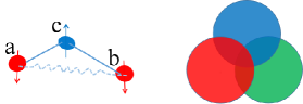
Figure 1: Left panel: Schematic diagram of three interacting qubits, solid lines represent the interaction between the blue spin $c$ and red spins $a$ or $b$. The curved line represents the entanglement between $a$ and $b$. Right panel: Schematic diagram of the entangled state manifold for the three interacting qubits. The mutual entanglements are symbolized by three color regions. The non-intersecting regions represent the separable state, the intersecting regions represent the entangled states.

Entanglement measures. Without loosing generality, here we consider the dynamical evolution of three interacting qubits by choosing an entangled qubit pair $ab$ as the initial state

$$|\Phi_{0}\rangle=\frac{1}{\sqrt{2}}(|\uparrow\downarrow\rangle_{ab}+|\downarrow\uparrow\rangle_{ab})\otimes|\uparrow\rangle_{c}.$$ (1)

For our convenience, we write initial state in the following form

$$|\Phi_{0}\rangle=\frac{1}{\sqrt{2}}(\mathbf{s_{a}^{-}}+\mathbf{s_{b}^{-}})|\Uparrow\rangle=\frac{1}{\sqrt{2}}(|a\rangle+|b\rangle)$$ (2)

with a notation $|x\rangle=s_{x}^{-}|\Uparrow\rangle$, where $s_{x}^{-}$ is spin-$1/2$ lowering operator and $|\Uparrow\rangle=|\uparrow\uparrow\uparrow\rangle$. See Fig. 1 left panel: two entangled qubits (red spins) have interaction with the third qubit (the blue one). Under a unitary time evolution, the wave function at arbitrary time can be written as

$$|\psi(t)\rangle=e^{-iHt}|\Phi_{0}\rangle.$$ (3)

We can also derive the density matrix of the model from the above wave function

$$\rho_{s}=|\psi(t)\rangle\langle\psi(t)|.$$ (4)

The density matrix is the key quantity to signal the entanglement dynamics transfer. In order to achieve this end, we calculate the quantum mutual information and the concurrence Nielsen; Wootters97; Wootters98; Wootters00. For example, the quantum mutual information and the concurrence of two qubits $a$ and $b$ are defined by

$$S(a:b)=S_{a}+S_{b}-S(a,b),$$ (5)

$$\mathcal{C}_{ab}=\max(0,\lambda_{1}-\lambda_{2}-\lambda_{3}-\lambda_{4}),$$ (6)

respectively. In the above equation, the Von Neumann entropy is given by $S(a,b)=-\Tr[\rho_{ab}\log_{2}\rho_{ab}]$, and $\{\lambda_{j}\}$ are square roots of the eigenvalues of the non-Hermitian matrix $\rho_{ab}\tilde{\rho}_{ab}$ in decreasing order, here $\tilde{\rho}_{ab}$ is defined by

$$\tilde{\rho}_{ab}=(\sigma_{y}\otimes\sigma_{y})\rho^{*}_{ab}(\sigma_{y}\otimes\sigma_{y}).$$

While $\rho_{x}$ denotes the reduced density matrix of a single qubit $x$.

Although forementioned entanglement measures are defined for two qubits, we can use the entanglement entropies of three qubit pairs to witness the three-qubit entanglement, see Fig. 1 right panel, in which three colour regions to symbolize the state manifold of three qubits. We observe the coexistence of the entanglement entropies of three qubit pairs $ab$, $ac$ and $bc$. The coexistence region presents a three-partite entanglement state, see Fig.2. We shall quantitatively study such mutual entanglement entropies below.

Inhomogeneous interacting qubits. Let’s first consider the entanglement dynamics of three interacting qubits with different spin exchange coupling, described by the Hamiltonian

$$H=2[A_{a}\mathbf{s_{a}}\mathbf{s_{c}}+A_{b}\mathbf{s_{b}}\mathbf{s_{c}}].$$ (7)

Here $A_{a,b}$ denote the spin exchange strengths for the qubit pairs $ac$ and and $bc$, respectively. The Hamiltonian (7) closely relates to the central spin model J.Dukelsky2004; H.-Q. Zhou; Dloss02; Dloss03; Bortz07; AFprb with the particle number $N=3$ and magnetic field $B=0$. Here the qubit $c$ play the role of the central spin. For our convenience, we introduce parameters $A_{j}=1/(\epsilon_{c}-\epsilon_{j})$, here $\epsilon_{c}=0$. We use the Bethe ansatz eigenfunction of the central spin model to investigate the time evolution of the system, namely,

$$|\{\nu\}\rangle=\prod_{\alpha=1}^{M}B_{\nu_{\alpha}}|\Uparrow\rangle=\prod_{\alpha=1}^{M}\sum_{j=a,b,c}\frac{s_{j}^{-}}{\nu_{\alpha}-\epsilon_{j}}|\Uparrow\rangle.$$ (8)

Here $j=a,b,c$ stands for the bath spins $a,b$, central spin $c$ and $M$ is the number of down-spins. The spectrum parameters $\{\nu\}$ satisfy the Bethe ansatz equations

$$\sum_{j=a,b,c}\frac{1}{\nu_{\alpha}-\epsilon_{j}}=\sum_{\beta\neq\alpha,\beta=1}^{M}\frac{2}{\nu_{\alpha}-\nu_{\beta}},$$ (9)

with $\alpha=1,\ldots,M$. The Bethe ansatz equations (9) have $C_{N}^{M}$ sets of solutions in the Hilbert subspace. For our case $M=1$, the eigenergy of the three qubits system reads

$$E=\frac{1}{2}\sum_{j=a,b}\frac{1}{\epsilon_{c}-\epsilon_{j}}-\frac{1}{\epsilon_{c}-\nu},$$ (10)

where the Bethe ansatz parameter $\nu$ satisfy the following equation

$$\frac{1}{\nu-\epsilon_{a}}+\frac{1}{\nu-\epsilon_{b}}+\frac{1}{\nu}=0,$$ (11)

that gives the solutions

$$\nu_{1,2}=\frac{1}{3}\left[(\epsilon_{a}+\epsilon_{b})\pm\sqrt{\epsilon_{a}^{2}+\epsilon_{b}^{2}-\epsilon_{a}\epsilon_{b}}\right],$$

$$\nu_{3}=\infty.$$

The solutions look rather simple, but indeed encode a rich quantum dynamics of three interacting qubits.

The initial state Eq. (1) belongs to the subspace with $M=1$. With the help of the above solutions, the wave function at arbitrary time can be obtained through the unitary evolution

$$|\psi(t)\rangle=e^{-iHt}|\Phi_{0}\rangle=\sum_{k}|\phi_{k}\rangle\langle\phi_{k}|\Phi_{0}\rangle e^{-iE_{k}t}.$$ (12)

Here orthonormalized eigenfunction $|\phi_{k}\rangle=N_{\nu_{k}}|\nu_{k}\rangle$, where $N_{\nu_{k}}$ is normalization factor

$$\frac{1}{{|N_{\nu_{k}}|}^{2}}\delta_{k,k^{\prime}}=\sum_{j=a,b,c}\frac{1}{(\nu_{k}-\epsilon_{j})(\nu_{k^{\prime}}-\epsilon_{j})}.$$

By a straightforward calculation of the overlap between eigenfunction and initial state, we obtain the time evolution of the wave function

$$|\psi(t)\rangle=\frac{1}{\sqrt{2}}\sum_{j=a,b,c}C_{j}(t)|j\rangle,$$ (13)

where coefficiences $C_{j}$ read

$$C_{j}(t)=\sum_{k}|N_{\nu_{k}}|^{2}\left[\frac{1}{\nu_{k}-\epsilon_{a}}+\frac{1}{\nu_{k}-\epsilon_{b}}\right]\frac{e^{-iE_{k}t}}{\nu_{k}-\epsilon_{j}}.$$

The next key step is to calculate the density matrix of system $\rho_{s}=|\psi(t)\rangle\langle\psi(t)|$. Again, using the wave function (13), we can obtain the density matrix

$$\rho_{s}=\left(\begin{array}[]{clr}{A(t)}/{2}&{D(t)}/{2}&{E(t)}/{2}\\ {D(t)^{*}}/{2}&{B(t)}/{2}&{F(t)}/{2}\\ {E(t)^{*}}/{2}&{F(t)^{*}}/{2}&{C(t)}/{2}\end{array}\right),$$ (14)

where the six coefficients are given by

$$A(t)= \sum\limits_{k}\sum\limits_{k^{\prime}}{|N_{\nu_{k}}|}^{2}{|N_{\nu_{k^{\prime}}}|}^{2}\left[\sum\limits_{\alpha=a,b}\frac{1}{\nu_{k}-\epsilon_{\alpha}}\right]\left[\sum\limits_{\alpha=a,b}\frac{1}{\nu_{k^{\prime}}-\epsilon_{\alpha}}\right]\frac{1}{(\nu_{k}-\epsilon_{a})(\nu_{k^{\prime}}-\epsilon_{a})}\cos(\omega_{kk^{\prime}}t),$$

$$B(t)= \sum\limits_{k}\sum\limits_{k^{\prime}}{|N_{\nu_{k}}|}^{2}{|N_{\nu_{k^{\prime}}}|}^{2}\left[\sum\limits_{\alpha=a,b}\frac{1}{\nu_{k}-\epsilon_{\alpha}}\right]\left[\sum\limits_{\alpha=a,b}\frac{1}{\nu_{k^{\prime}}-\epsilon_{\alpha}}\right]\frac{1}{(\nu_{k}-\epsilon_{b})(\nu_{k^{\prime}}-\epsilon_{b})}\cos(\omega_{kk^{\prime}}t),$$

$$C(t)= \sum\limits_{k}\sum\limits_{k^{\prime}}{|N_{\nu_{k}}|}^{2}{|N_{\nu_{k^{\prime}}}|}^{2}\left[\sum\limits_{\alpha=a,b}\frac{1}{\nu_{k}-\epsilon_{\alpha}}\right]\left[\sum\limits_{\alpha=a,b}\frac{1}{\nu_{k^{\prime}}-\epsilon_{\alpha}}\right]\frac{1}{(\nu_{k}-\epsilon_{c})(\nu_{k^{\prime}}-\epsilon_{c})}\cos(\omega_{kk^{\prime}}t),$$

$$D(t)= \sum\limits_{k}\sum\limits_{k^{\prime}}{|N_{\nu_{k}}|}^{2}{|N_{\nu_{k^{\prime}}}|}^{2}\left[\sum\limits_{\alpha=a,b}\frac{1}{\nu_{k}-\epsilon_{\alpha}}\right]\left[\sum\limits_{\alpha=a,b}\frac{1}{\nu_{k^{\prime}}-\epsilon_{\alpha}}\right]\frac{1}{(\nu_{k}-\epsilon_{a})(\nu_{k^{\prime}}-\epsilon_{b})}e^{i\omega_{kk^{\prime}}t},$$

$$E(t)= \sum\limits_{k}\sum\limits_{k^{\prime}}{|N_{\nu_{k}}|}^{2}{|N_{\nu_{k^{\prime}}}|}^{2}\left[\sum\limits_{\alpha=a,b}\frac{1}{\nu_{k}-\epsilon_{\alpha}}\right]\left[\sum\limits_{\alpha=a,b}\frac{1}{\nu_{k^{\prime}}-\epsilon_{\alpha}}\right]\frac{1}{(\nu_{k}-\epsilon_{a})(\nu_{k^{\prime}}-\epsilon_{c})}e^{i\omega_{kk^{\prime}}t},$$

$$F(t)= \sum\limits_{k}\sum\limits_{k^{\prime}}{|N_{\nu_{k}}|}^{2}{|N_{\nu_{k^{\prime}}}|}^{2}\left[\sum\limits_{\alpha=a,b}\frac{1}{\nu_{k}-\epsilon_{\alpha}}\right]\left[\sum\limits_{\alpha=a,b}\frac{1}{\nu_{k^{\prime}}-\epsilon_{\alpha}}\right]\frac{1}{(\nu_{k}-\epsilon_{b})(\nu_{k^{\prime}}-\epsilon_{c})}e^{i\omega_{kk^{\prime}}t},$$

with the frequency $\omega_{kk^{\prime}}=1/(\nu_{k}-\epsilon_{c})-1/(\nu_{k^{\prime}}-\epsilon_{c})$.

By tracing out the third qubit, the reduced density matrices of three qubit pairs $\rho_{ab},\rho_{ac},\rho_{bc}$ read

$$\rho_{ab} = \frac{C(t)}{2}|\uparrow\uparrow\rangle\langle\uparrow\uparrow|+\frac{B(t)}{2}|\uparrow\downarrow\rangle\langle\uparrow\downarrow|+\frac{A(t)}{2}|\downarrow\uparrow\rangle\langle\downarrow\uparrow|$$

$$+\frac{D^{*}(t)}{2}|\uparrow\downarrow\rangle\langle\downarrow\uparrow|+\frac{D(t)}{2}|\downarrow\uparrow\rangle\langle\uparrow\downarrow|,$$

$$\rho_{ac} = \frac{B(t)}{2}|\uparrow\uparrow\rangle\langle\uparrow\uparrow|+\frac{C(t)}{2}|\uparrow\downarrow\rangle\langle\uparrow\downarrow|+\frac{A(t)}{2}|\downarrow\uparrow\rangle\langle\downarrow\uparrow|$$

$$+\frac{E^{*}(t)}{2}|\uparrow\downarrow\rangle\langle\downarrow\uparrow|+\frac{E(t)}{2}|\downarrow\uparrow\rangle\langle\uparrow\downarrow|,$$

$$\rho_{bc} = \frac{A(t)}{2}|\uparrow\uparrow\rangle\langle\uparrow\uparrow|+\frac{C(t)}{2}|\uparrow\downarrow\rangle\langle\uparrow\downarrow|+\frac{B(t)}{2}|\downarrow\uparrow\rangle\langle\downarrow\uparrow|$$

$$+\frac{F^{*}(t)}{2}|\uparrow\downarrow\rangle\langle\downarrow\uparrow|+\frac{F(t)}{2}|\downarrow\uparrow\rangle\langle\uparrow\downarrow|.$$

Moreover, it’s easy to diagonalize the above three matrices to get their eigenvalues. The reduced density matrices of single qubit $\rho_{a},\rho_{b},\rho_{c}$ are given by

$$\rho_{a}= (B(t)/2+C(t)/2)|\uparrow\rangle\langle\uparrow|+A(t)/2|\downarrow\rangle\langle\downarrow|,$$

$$\rho_{b}= (A(t)/2+C(t)/2)|\uparrow\rangle\langle\uparrow|+B(t)/2|\downarrow\rangle\langle\downarrow|,$$

$$\rho_{c}= (A(t)/2+B(t)/2)|\uparrow\rangle\langle\uparrow|+C(t)/2|\downarrow\rangle\langle\downarrow|.$$

Using the definition of entanglement measures (5) and (6), we obtain the quantum mutual information and concurrence, for example the qubit pair $ab$

$$S(a:b) =\gamma_{1}\log_{2}\gamma_{1}+\gamma_{2}\log_{2}\gamma_{2}+\gamma_{3}\log_{2}\gamma_{3}-A\log_{2}A$$

$$-B\log_{2}B-(\frac{A}{2}+\frac{C}{2})\log_{2}(\frac{A}{2}+\frac{C}{2})$$

$$-(\frac{B}{2}+\frac{C}{2})\log_{2}(\frac{B}{2}+\frac{C}{2}),$$ (15)

$$\mathcal{C}_{ab} =\max(0,{\lambda_{1}}-{\lambda_{2}}).$$ (16)

Above parameters $\{\gamma_{i}\}$ and $\{\lambda_{i}\}$ are respectively the eigenvalues of the density matrix $\rho_{ab}$ and square roots of the matrix $\rho_{ab}\tilde{\rho}_{ab}$ in decreasing order

$$\gamma_{1,2}=\frac{A+B}{4}\pm\frac{1}{4}\sqrt{(A-B)^{2}+|D|^{2}}],$$

$$\gamma_{3}=\frac{C}{2},$$

$$\lambda_{1,2}^{2}=\frac{1}{4}[(AB+|D|^{2})\pm\sqrt{4AB|D|^{2}}].$$

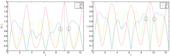
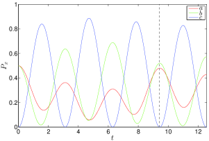
Figure 2: The entanglement dynamics of three qubits with different pairwise interactions. Left panel: Quantum mutual informations of three qubit pairs evolve in time. Right panel: Concurrences of three qubit pairs evolve in time. The red line is the entanglement dynamics of the qubit pair $ab$, the blue line stands for the entanglement dynamics of the qubit pair $ac$, whereas the green line denotes the entanglement dynamics of the qubit pair $bc$. Irregular oscillation of the entanglement dynamics transfers was observed in both the mutual information and concurrence. The black dashed lines show a nearly perfect revival time of the initial state.

Figure 3: The probability of state $|x\rangle$ evolves in time for the inhomogeneous Hamiltonian (7). The different color lines show the probabilities of different states $|a,b,c\rangle$, Here the coupling constant $A_{a}=0.5,A_{b}=0.8$. The back dashed line shows a nearly perfect revival time of the initial state.

From Fig.2, we observe that the time evolutions of quantum mutual information and concurrence show a coherence transfer behaviour. Initially starting from the entangled state of the qubit pair $ab$, such a dynamics transfer displays asymmetric feature, i.e. the entanglement entropy and concurrence of the qubit pairs $ac$ and $bc$ oscillate with different frequencies and different magnitudes. Due to the presence of the inhomogeneous pairwise interactions, there does not exist triple intersection point in time evolution of the entanglement dynamics. There are the regions where the entanglements of three qubit pairs are nearly same, see the marked black circles in Fig. 2.

The probability of state $|x\rangle$ with $x\in\{a,b,c\}$, is defined as

$$P_{x}=\Tr[\rho_{s}|x\rangle\langle x|],$$ (17)

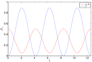
that measures the probability of projecting the state $\psi(t)$ onto the state $|x\rangle$. In Fig. 3, we show the probabilities of the states $|a\rangle$,$|b\rangle$,$|c\rangle$. They oscillate anharmonically. A nearly perfect revival of the probabilities of the three states shows the time $t\approx 9.4$ (dashed line) which is exactly the same as the nearly revival time of the entropy dynamics, see Fig. 2. This means that at this time the qubit $c$ gets disentangled from the other two qubits. However, the system does not completely return back initial state, since the probability of states $|a\rangle$ and $|b\rangle$ are nearly equal. The result originates from both the monogamy of the entanglement of qubit pair $ab$ and the asymmetric pairwise interactions.

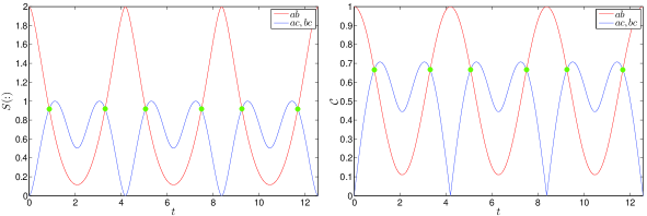
Figure 4: Entanglement dynamics of three qubits for the homogenous Hamiltonian (18). Left panel: Quantum mutual information of three qubit pairs $ab,ac,bc$ evolves time. Right panel: Concurrence of three qubit pairs $ab,ac,bc$ evolves in time. The red lines show the entanglement of the qubit pair $ab$. The blue lines show the entanglement of the qubit pairs $ac$ and $bc$. The green dots mark the triple intersection points, i.e. three qubit pairs have the equal mutual information and concurrence.

Homogeneous case. We now consider the homogenous three interacting qubits with the Hamiltonian

$$H=J[\mathbf{s_{a}}\mathbf{s_{c}}+\mathbf{s_{b}}\mathbf{s_{c}}].$$ (18)

Here we set the coupling constant $J=1$ for a dimensionless unit. The Hamiltonian (18) can be regarded as a three-qubit-Heisenberg chainXiaoGwang, whose dynamics can be obtained by the integrable model natan2014. Now we may calculate the wave function by using a recurrence relation, namely,

$$|\psi(t)\rangle=\frac{1}{\sqrt{2}}e^{-iHt}(|a\rangle+|b\rangle)$$

$$=\frac{1}{\sqrt{2}}[\sum_{n=0}^{\infty}\frac{(-it)^{n}}{n!}H^{n}(|a\rangle+|b\rangle)]$$

$$=\frac{1}{\sqrt{2}}[\sum_{n=1}^{\infty}\frac{(-it)^{n}}{n!}H^{n-1}|c\rangle+(|a\rangle+|b\rangle)].$$

By acting the Hamiltonian (18) on state $|c\rangle$ continuously, we further find a useful structure for getting the spectrum of the model

$$H^{n}|c\rangle=|c_{1}\rangle\alpha_{1}^{n}+|c_{2}\rangle\alpha_{2}^{n},$$

with $\alpha_{1}=-1,\alpha_{2}=\frac{1}{2}$. In the above equation the two states are defined by $|c_{1}\rangle=\frac{2}{3}|c\rangle-\frac{1}{3}|a\rangle-\frac{1}{3}|b\rangle$ and $|c_{2}\rangle=\frac{1}{3}|c\rangle+\frac{1}{3}|a\rangle+\frac{1}{3}|b\rangle$, where the three basises $|a\rangle=\left(\begin{array}[]{clr}1&0&0\end{array}\right)^{t}$, $|b\rangle=\left(\begin{array}[]{clr}0&1&0\end{array}\right)^{t}$, $|c\rangle=\left(\begin{array}[]{clr}0&0&1\end{array}\right)^{t}$. Thus the wave function at arbitrary time is given by

$$|\psi(t)\rangle=\frac{1}{\sqrt{2}}\left[\frac{e^{-i\alpha_{1}t}}{\alpha_{1}}|c_{1}\rangle+\frac{e^{-i\alpha_{2}t}}{\alpha_{2}}|c_{2}\rangle\right].$$ (19)

From this wave function, the density matrix of system is obtained directly

$$\rho_{s}=\left(\begin{array}[]{clr}A(t)&A(t)&B(t)\\ A(t)&A(t)&B(t)\\ B^{*}(t)&B^{*}(t)&C(t)\end{array}\right).$$ (20)

Three matrix elements $A,B,C$ are respectively given

$$A(t) =\frac{1}{2}\left[\frac{1}{9\alpha_{2}^{2}}+\frac{1}{9\alpha_{1}^{2}}-\frac{2\cos[(\alpha_{2}-\alpha_{1})t]}{9\alpha_{1}\alpha_{2}}\right],$$

$$B(t) =\frac{1}{2}\left[\frac{1}{9\alpha_{2}^{2}}-\frac{2}{9\alpha_{1}^{2}}+\frac{2e^{\mathrm{i}(\alpha_{1}-\alpha_{2})t}}{9\alpha_{1}\alpha_{2}}-\frac{e^{\mathrm{i}(\alpha_{2}-\alpha_{1})t}}{9\alpha_{1}\alpha_{2}}\right],$$

$$C(t) =\frac{1}{2}\left[\frac{1}{9\alpha_{2}^{2}}+\frac{4}{9\alpha_{1}^{2}}+\frac{4\cos[(\alpha_{2}-\alpha_{1})t]}{9\alpha_{1}\alpha_{2}}\right].$$

We further obtain the reduced density matrices of three qubit pairs $\rho_{ab},\rho_{ac},\rho_{bc}$ by tracing out the third qubit

$$\rho_{ab}= C(t)|\uparrow\uparrow\rangle\langle\uparrow\uparrow|+A(t)|\uparrow\downarrow\rangle\langle\uparrow\downarrow|+A(t)|\downarrow\uparrow\rangle\langle\downarrow\uparrow|$$

$$+A(t)|\uparrow\downarrow\rangle\langle\downarrow\uparrow|+A(t)|\downarrow\uparrow\rangle\langle\uparrow\downarrow|,$$

$$\rho_{ac}= A(t)|\uparrow\uparrow\rangle\langle\uparrow\uparrow|+C(t)|\uparrow\downarrow\rangle\langle\uparrow\downarrow|+A(t)|\downarrow\uparrow\rangle\langle\downarrow\uparrow|$$

$$+B^{*}(t)|\uparrow\downarrow\rangle\langle\downarrow\uparrow|+B(t)|\downarrow\uparrow\rangle\langle\uparrow\downarrow|,$$

$$\rho_{bc}= A(t)|\uparrow\uparrow\rangle\langle\uparrow\uparrow|+C(t)|\uparrow\downarrow\rangle\langle\uparrow\downarrow|+A(t)|\downarrow\uparrow\rangle\langle\downarrow\uparrow|$$

$$+B^{*}(t)|\uparrow\downarrow\rangle\langle\downarrow\uparrow|+B(t)|\downarrow\uparrow\rangle\langle\uparrow\downarrow|.$$

Note that here we used the same notations for these functions $A(t),\,B(t),\,C(t)$ as being used in the inhomogeneous case.

It’s easy to diagonalize the above three matrices to obtain their eigenvalues. Moreover, the reduced density matrices of the single qubit $\rho_{a},\,\rho_{b},\,\rho_{c}$ are given by

$$\rho_{a}= (A(t)+C(t))|\uparrow\rangle\langle\uparrow|+A(t)|\downarrow\rangle\langle\downarrow|,$$

$$\rho_{b}= (A(t)+C(t))|\uparrow\rangle\langle\uparrow|+A(t)|\downarrow\rangle\langle\downarrow|,$$

$$\rho_{c}= 2A(t)|\uparrow\rangle\langle\uparrow|+C(t)|\downarrow\rangle\langle\downarrow|.$$

There are only diagonal elements in the reduced density matrix of single qubits $\rho_{a},\rho_{b},\rho_{c}$ due to the conserved magnetization. Accoding to the definition of entanglement measure, for instance, the quantum mutual information and concurrence of qubit pair $ab$

$$S(a:b) =2A+C\log_{2}C-2(A+C)\log_{2}(A+C),$$ (21)

$$\mathcal{C}_{ab} =\max(0,2A).$$ (22)

We also can derive the probabilities $P_{a,b,c}$ of the three states like what discussed in the inhomogeneous case.

Figure 5: The probability of state $|x\rangle$ evolve with time for homogeneous case. The red line is the probability of state $|a\rangle$ or $|b\rangle$, blue line is the probability of state $|c\rangle$

Fig.4 shows the entanglement entropy and concurrence of the homogenous Hamiltonian (18). We observe that the genuine three-qubit entangled state is naturally induced through two pairwise interactions $ac$ and $bc$. There exist some special states at which the entanglements of three qubit pairs are the same, see the marked green dots in Fig. 4. The times when the three pairwise entangled states are equal satisfy the relation $t_{e}=\pm\frac{2}{3}\arccos(\frac{1}{4})+\frac{4}{3}n\pi$, here $n\in\{0,1,2,\cdots\}$. While at these points the probabilities of the single states $|a\rangle$,$|b\rangle$,$|c\rangle$ are also the same, see Fig. 5. In contrast to the inhomogenous case Fig. 3, the probability $P_{a},P_{b},P_{c}$ oscillate periodically due to the homogeneous pairwise interaction. The state consisting of three equally entangled states is called the $W$ state, where the three qubits are a equally weighted superposition and the norm of the off-diagonal element $B$ in density matrix is $1/3$. We can prove that the quantum mutual information of the equally entangled state is same as the quantum mutual information of the $W$ state with the entanglement entropy $S_{w}=\log_{2}(3)-\frac{2}{3}\approx 0.9183$ for two qubits pair. It is also easy to check the concurrence $\mathcal{C}=\frac{2}{3}$ for both. This is a very interesting feature that dynamical evolution of the pairwise entangled state can produce a three-partite entangled $W$ state. In contrast to the smooth time evolution of the quantum mutual information, the concurrence shows sharp changes at certain times, see the blue line in the right panel of Fig. 4. The evolutions of quantum mutual information and concurrence reveal a very interesting features of quantum entanglement transfer.

Experimental Proposal Finally, we propose an experimental scheme to test the above entanglement dynamics by using Rydberg atom M. Saffman. One can use three ⁸⁷Rb atoms to simulate the entanglement dynamics transfer in the homogeneous Hamiltonian (18) and use two ⁸⁷Rb atoms and one ${}^{23}Na$ atom or three heteronuclear Rb atoms to simulate the such a dynamics transfer in the inhomogeneous Hamiltonian (7). For the homogeneous case, we estimate the time of the first equally entangled state point, $t_{1}=\frac{2}{3J}\arccos(\frac{1}{4})\approx 0.8787/J$. Here we used the data of spin exchange coupling constant given in Barredo:2015. The spin exchange coupling reads $J=C_{3}^{\exp}/R^{3}$ with the parameter setting $C_{3}^{\exp}=7950\pm 130\MHz{\mu m}^{3},R=30\mu m$. Thus the estimated time of the first equally entangled state is at $t_{1}\approx 2.9843\mu s$, which can be accessible experimentally.

In summary. We have studied the quantum entanglement dynamics transfer in three pairwise interacting qubits. We have analytically calculated time evolutions of wave function, density matrix and entanglement entropy for the system. We have found that pairwise interactions may induce a genuine three-qubit entangled state during time evolution. In such a three-qubit entangled state, the mutual entanglement entropies can be equally weighted depending on the choices of the pairwise interactions. The evolution of quantum mutual information is a smooth function of time. The concurrence displays some sharp changes at some points. The entanglement dynamics transfer in the inhomogeneous system is anharmonic. In this case, the initial state can not completely return back even the entanglement of the initial qubit pair $ab$ reaches the maximum.

Acknowledgments. This work is supported by the key NSFC grant No. 11534014 and the National Key R&D Program of China No. 2017YFA0304500.

References

(1) Barredo D, Labuhn H, Ravets S, Lahaye T , Browaeys A, and Adams C S 2015 Phys. Rev. Lett 114 113002
(2) Rosenfeld E L , Pham L M , Lukin M D and Walsworth R L 2018 Phys. Rev. Lett 120 243604
(3) Polkovnikov A , Sengupta K, Silva A , and Vengalattore M 2011 Rev. Mod. Phys. 83 863
(4) Amico L , Fazio R, Osterloh A , and Vedral V 2008 Rev. Mod. Phys. 80 517
(5) Giovannetti V , Lloyd S , and Maccone L 2006 Phys. Rev. Lett. 96 010401
(6) Li X K , Zhu B , He X D , Wang F D, Guo M Y, Xu Z F , Zhang S Z , and Wang D J 2015 Phys. Rev. Lett. 114 255301
(7) Zeng Y , Xu P , He X D , Liu Y Y, Liu M , Wang J, Papoular D J, Shlyapnikov G V , and Zhan M S 2017 Phys. Rev. Lett. 119 160502
(8) DiCarlo L, Reed M D, Sun L, Johnson B R , Chow J M , Gambetta J M , Frunzio L , Girvin S M , Devoret M H and Schoelkopf R J 2010 Nature 467 574–578
(9) Wang B C , Cao G , Li H O , Xiao M , Guo G C , Hu X D , Jiang H W , and Guo G P 2017 Phys. Rev. Applied. 8 064035
(10) Nielsen M A and Chuang I L , Quantum Computation and Quantum Information (Cambridge University Press, Cambridge, England, 2000).
(11) Hill S and Wootters W K 1997 Phys. Rev. Lett. 78 5022
(12) Wootters W K 1998 Phys. Rev. Lett. 80 2245
(13) Coffman V, Kundu J and Wootters W K 2000 Phys. Rev. A. 61 052306
(14) Dukelsky J, Pittel S, Sierra G 2004 Rev. Mod. Phys. 76, 643
(15)Zhou H Q, Links J , McKenzie R H , and Gould M D 2002 Phys. Rev. B. 65 060502(R)
(16) Khaetskii A V, Loss D, Glazman L 2002 Phys. Rev. Lett. 88 18
(17) Khaetskii A V, Loss D, Glazman L 2003 Phys. Rev. B. 67 195329
(18) Bortz M, Stolze J 2007 Phys. Rev. B. 76 014304
(19) Araby O E , Gritsev V , and Faribault A 2012 Phys. Rev. B. 85 115130
(20) Wang X G 2001 Phys. Rev. A. 64 012313
(21) Liu W S , Andrei N 2014 Phys. Rev. Lett. 112 257204
(22) Saffman M, Walker T G, and Mlmer K 2010 Rev. Mod. Phys. 82 2313