Introduction to Regge Calculus for Gravitation

Abstract

With the theory of general relativity, Einstein abolished the interpretation of gravitation as a force and associated it to the curvature of spacetime. Tensorial calculus and differential geometry are the mathematical resources necessary to study the spacetime manifold in the context of Einstein’s theory. In 1961, Tullio Regge published a work on which he uses the old idea of triangulation of surfaces aiming the description of curvature, and, therefore, gravitation, through the use of discrete calculus. In this paper, we approach Regge Calculus pedagogically, as well as the main results towards a discretized version of Einstein’s theory of gravitation.

Instituto de Ciência e Tecnologia, Universidade Federal de Alfenas
BR 267 – Rodovia José Aurélio Vilela, 11999, CEP 37701-970, Poços de Caldas, MG, Brazil

1 Introduction

Since the ancient Greeks, the method of decomposing a complicated problem in simpler parts is one of the fundamental pillars of science development. Indeed, it is possible to consider this abstraction as one of the techniques of logical thought since it permeates natural science including mathematics.

Democritus (c.460 BC) introduced the idea of decomposing a complex object into fundamental indivisible and smaller pieces, and it took almost 2,500 years for this proposal being coherently implemented by Quantum Mechanics. We can find a similar type of reasoning in the efforts of Eudoxus (408-255 BC) in his efforts to calculate areas using the Method of Exhaustion. The exhaustion method has a relation to the Finite Element Method and the graphics computational methods used to smooth out surfaces.

Regge Calculus [1, 2] is an additional element of this set of discretization methods applied to the description of space-time. Tullio Regge’s ideas were to build the smooth spacetime manifold without using coordinates. Instead, he used basic concepts of topology. Once these concepts are more familiar in three dimensions, Regge uses the method of “Euclidianization”, where some geometrical quantities of the theory assume complex values . Thereby, he demonstrated the results in two or three dimensions from which the conclusion could be generalized to four dimensions.This strategy is pedagogically resourceful and will be used in this paper.

The same way as the basic elements of matter receive a special name – atoms –, there is a denomination for the fundamental elements of geometry in Regge Calculus: simplexes. A simplex is the spacetime manifold fundamental building-block. For example, think of a two-dimension surface like a wall. The simplexes would be the tiles or mosaics used to cover it. There is no need for the tiles to be of the same form or size (contrary to what commonly happens to the usual tiling in a house), but they should match like the pieces in a puzzle, they should be self-joining in a way that covers the whole surface. Maurice Escher masterfully illustrated this reasoning, e.g. Fig. 1.

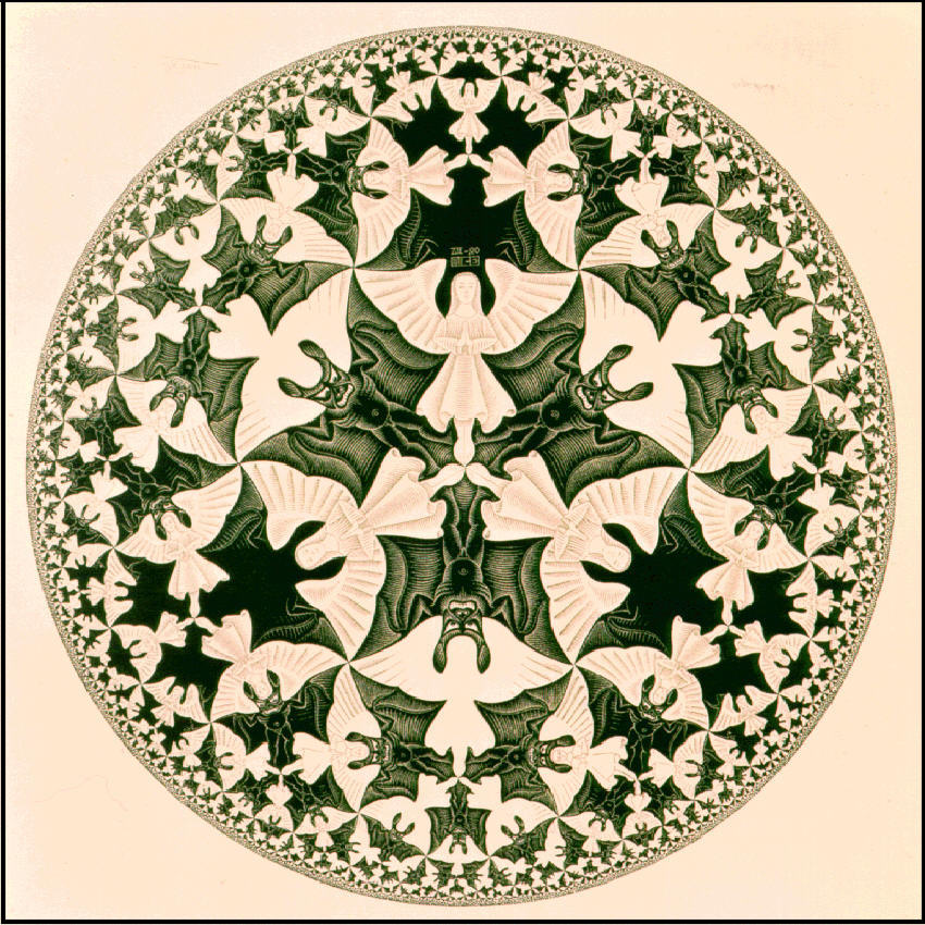
Figure 1: The work “Circle Limit IV: Heaven and Hell” by M.C. Escher (dated 1960) exemplifies the overlay of a surface by mosaics with different characteristics.

2 The Discretization of Space

Einstein’s equations for gravitation supply a systematic way to determine the geometry of spacetime, which is generally curved. Given a particular distribution of matter described by the energy-momentum tensor, it is possible in principle to calculate the independent components of the metric by solving a nonlinear system of coupled differential equations. In fact, it is only possible to obtain the solutions analytically when the degree of symmetry of matter distribution is high. This fact restricts vertiginously the collection of solutions we have access to without calling upon numerical resources. This difficulty motivates the search for an alternative method to general relativity to describe the curvature of spacetime.

Regge’s work [1] lays down such an alternative, even though his motivation might have been the solution to mathematical problems in areas such as in topology, homology, holonomy, and homotopy [3]. Regge proposes the discretization of a continuous and smooth manifold into Euclidian simplexes (polyhedrons). The triangulation of the manifold carries a similarity with the homology methods (as in Ref. [4], Chapter 2). Fig. 2 is consistent with this scenario: The picture shows a hemispherical dome that protects Atibaia’s radio telescope in Brazil; the dome is composed of a multitude of plane triangles connected edge to edge and vertex to vertex.

Figure 2: The dome protecting Itapetinga $13.4\operatorname{m}$ radio telescope at Atibaia (Brazil) is an example of discretization of a curved surface by a set of juxtaposed plane polygons.

The surface triangulation starts by choosing the base simplex (the fundamental shape for the covering polygons). The idea is to take the polyhedrons as similar as possible to regular simplexes (of equal edges). However, it is not possible to maintain all the sides with the same length, because we need to accommodate some degree of freedom to fit the curved surface. The number of required simplexes depends on the magnitude of the surface’s curvature. The more intensely the surface bends, the greater is the number of simplexes necessary to cover it. Also, the higher the density of simplexes (number of simplexes per unity area), the better is the approximation achieved with the discretization process.

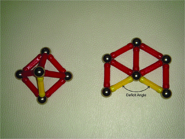
Figure 3: The pyramid simplex (3D) – on the left – could be cut off along the yellow edge and be flattened (2D). This way is possible to show the deficit angle associated with the vertex.

Since the elements of the lattice covering the manifold are flat, one might ask: Where is the curvature concentrated? The answer is: Curvature is measured at the vertexes. There is no curvature in between the edges of the adjacent triangles. In fact, consider the point on the tip of a pyramid – Fig. 3 (ignore the horizontal basis for the sake of the argument). It is possible to flatten this surface if, and only if, we cut through along one of the edges that go up to the top $\mathcal{V}$. In this scenario, the sum of the dihedral angles $\theta_{n}$ (in the $n$ triangles) around $\mathcal{V}$ will not be $2\pi$ in the flatten surface, as it would be expected in the plane formed of triangles. There will be an angular difference $\varepsilon$,

$$\varepsilon=2\pi-\sum_{n}\theta_{n}\,,$$

measuring the curvature of the pyramidal surface. Note that we do not measure any deficit angle when traversing adjoint triangles on the flattened surface except when crossing the edge along with we cut off till the apex, showing that the vertex represents the curvature.

Incidentally, there are many vertexes in a complex surface, each one with its associated angular deficit $\varepsilon$ characterizing the local curvature. It is in this general surface that we start our quantitative study.

3 Curvature

There are several polyhedrons around each one of the $M$ vertexes of a discretized manifold. The number of polyhedrons is large if the magnitude of the local curvature is large. These polyhedrons touch one another, and the touching edges form a bundle of many parallel edges – or bones. This bundle is a joint, designated by the letter $p$; there is a large number $P$ of joints throughout the manifold. These $P$ joints have a average bone density $\varrho$.

Figure 4: A particular joint $p$: bundle composed of $r$ edges ($r=5$).

Fig. 4 shows a specific joint $p$. There is a related bundle of bone of density $\varrho_{p}$ oriented by the unity vector $\mathbf{U}^{p}\left(\equiv\mathbf{U}_{p}\right)$ which is parallel to a member of the bundle and points to the vertex, i.e.,

$$\mathbf{U}^{p}=U^{p}\leavevmode\nobreak\ \mathbf{n}_{p}\,;\leavevmode\nobreak\ \ \ \ U_{\mu}^{p}U_{p}^{\mu}=1\,.$$ (1)

We define the components of $\mathbf{U}^{p}$ with respect to a Cartesian coordinate system fixed in the manifold. This choice of reference frame is always possible because the hyper-surface is a piecewise-Euclidean manifold.

According to the discussion in Sect. 2, the curvature in joint $p$ is concentrated at the vertex $m$ and the deficit angle $\varepsilon_{p}$ quantifies it. In the case of continuous manifolds of General Relativity, the Riemann tensor $R_{\leavevmode\nobreak\ \nu\alpha\beta}^{\mu}$ quantifies spacetime curvature. It is necessary to study the parallel transport of a vector $\mathbf{A}$ along an infinitesimal closed loop in order to relate the discretized manifold $\varepsilon_{p}$ with the continuous manifold $R_{\leavevmode\nobreak\ \nu\alpha\beta}^{\mu}$. A loop in a continuous (Riemannian) manifold is represented in Fig. 5.

Figure 5: Parallel transport of $\mathbf{A}$ in a Riemannian manifold with the approximate shape of a quarter hemisphere (on the left). The vector goes from position $1$ to position $1^{\prime}$ after the displacement $1\rightarrow 2\rightarrow 3\rightarrow 1^{\prime}$. Note $\mathbf{A}$ appears rotated with respect to its original position (as indicated on the right): the rotation angle is $\sigma$; $\vec{\sigma}$ is the associated vector built from the unity vector $\hat{n}_{p}$ which is ortogonal to the plane containing $1$ and $1^{\prime}$. (Adapted from Ref. [5].)

Vector $\mathbf{A}$ rotates with respect to its initial position, throughout the process of being transported. This rotation is the disclination property of the curved space.

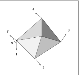
Figure 6: Parallel transport of a vector around a set of simplexes.

The loop in our discretized (simplex) case is taken to be, say, around the bundle $p$. Let $\Sigma$ be the area enclosed by this loop. If $\mathbf{n}_{\Sigma}$ is an unity vector ortogonal to this area, then

$$\mathbf{\Sigma}=\Sigma\leavevmode\nobreak\ \mathbf{n}_{\Sigma}$$ (2)

is the area vector associated to that path. The closed path goes around the simplex polyhedrons that gather at the bundle $p$, cf. Fig. 6. At the end of its displacement along the path $1\rightarrow 2\rightarrow 3\rightarrow 4\rightarrow 1^{\prime}$, vector $\mathbf{A}$ rotates by an angle $\mathbf{\sigma}$,

$$\vec{\sigma}=\sigma\leavevmode\nobreak\ \mathbf{n}_{p}=\sigma\leavevmode\nobreak\ \mathbf{U}_{p}\,,$$ (3)

pointing along the bundle of bones around which $\mathbf{A}$ rotates. Vetor $\mathbf{A}$ turns to:

$$\mathbf{\bar{A}}=\mathbf{A}+\delta\mathbf{A}\,.$$

Figure 7: Rotation of $\mathbf{A}$ after the parallel transport around a loop in the discretized manifold produces vector $\bar{\mathbf{A}}$. Vector $\mathbf{\sigma}\equiv\vec{\sigma}$ is pointing outward the plane of the page containing both $\mathbf{A}$ and $\bar{\mathbf{A}}$; it gives direction to the rotation angle $\sigma$.

Since the rotation is “infinitesimal”, the “arc” $\delta\mathbf{A}$ has magnitude $\delta A=\sigma A$. This is displayed in Fig. 7. The associated vector is:

$$\delta\mathbf{A}=\mathbf{\sigma}\times\mathbf{A}\,.$$ (4)

Angle $\sigma$ must be directly proportional to the curvature which is described by the deficit angle $\varepsilon_{p}$. The proportionality constant is precisely the number of bones embraced by the loop, $N$:

$$\sigma=N\leavevmode\nobreak\ \varepsilon_{p}\,.$$ (5)

The reason for that was mentioned before: The higher the number of simplexes $N$ associated to the vertex $p$ the more significant the curvature and the higher the angular displacement of $\mathbf{A}$.

By the way, $N$ is the product of the density of bones in the joint, $\varrho_{p}$, by the area resulting from the projection of $\mathbf{\Sigma}$ in the direction of $\mathbf{U}$:

$$N=\varrho_{p}\leavevmode\nobreak\ \left(\mathbf{U}_{p},\mathbf{\Sigma}\right)=\varrho_{p}\leavevmode\nobreak\ \mathbf{U}_{p}\cdot\mathbf{\Sigma}\,,$$ (6)

where the symbol $(\,\,,\,)$ denotes the internal product operation; its is simply the dot product $(\cdot)$ in the context of vector algebra. (The component of $\mathbf{A}$ along the perpendicular direction to the bundle does not generate contributions to $\vec{\sigma}$.) Fig. 8 sketches the projection achieved by Eq. (6).

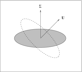
Figure 8: Projection of the oriented area $\mathbf{\Sigma}$ onto the direction of vector $\mathbf{U}$ pointing along the bundle of bones.

By substituting (3), (5) and (6) into (4), we obtain the change $\mathbf{A}$ suffered under the parallel transport in the discretized manifold:

$$\delta\mathbf{A}=\varrho_{p}\leavevmode\nobreak\ \varepsilon_{p}\leavevmode\nobreak\ \left(\mathbf{U}_{p}\cdot\mathbf{\Sigma}\right)\leavevmode\nobreak\ \left(\mathbf{U}_{p}\times\mathbf{A}\right)\,.$$ (7)

This equation can be expressed in terms of vector components:

$$\delta A^{\mu}=\varrho_{p}\leavevmode\nobreak\ \varepsilon_{p}\leavevmode\nobreak\ \left(U_{p}^{\leavevmode\nobreak\ \nu}\Sigma_{\nu}\right)\leavevmode\nobreak\ \left(\epsilon^{\mu\alpha\beta}U_{\leavevmode\nobreak\ \alpha}^{p}A_{\beta}\right)\,,$$ (8)

where $\epsilon^{\mu\alpha\beta}$ is the totaly antisymmetric Levi-Civita symbol (or permutation symbol):

$$\epsilon^{123} \equiv+1\,;$$

$$\epsilon^{\alpha\beta\gamma} =\epsilon^{\gamma\alpha\beta}=\epsilon^{\beta\gamma\alpha}\,;$$ (9)

$$\epsilon^{\alpha\beta\gamma} =-\epsilon^{\beta\alpha\gamma}=-\epsilon^{\alpha\gamma\beta}\,.$$

A compact realization of all the features in Eq. (9) is:

$$\epsilon_{\alpha\beta\gamma} =\delta_{\alpha}^{1}\delta_{\beta}^{2}\delta_{\gamma}^{3}+\delta_{\beta}^{1}\delta_{\gamma}^{2}\delta_{\alpha}^{3}+\delta_{\gamma}^{1}\delta_{\alpha}^{2}\delta_{\beta}^{3}+$$

$$-\delta_{\alpha}^{1}\delta_{\gamma}^{2}\delta_{\beta}^{3}-\delta_{\gamma}^{1}\delta_{\beta}^{2}\delta_{\alpha}^{3}-\delta_{\beta}^{1}\delta_{\alpha}^{2}\delta_{\gamma}^{3}\,.$$ (10)

Then,

$$\epsilon_{\alpha\beta\gamma}\epsilon^{\mu\nu\gamma}=\left(\delta_{\leavevmode\nobreak\ \alpha}^{\mu}\delta_{\leavevmode\nobreak\ \beta}^{\nu}-\delta_{\leavevmode\nobreak\ \beta}^{\mu}\delta_{\leavevmode\nobreak\ \alpha}^{\nu}\right)\,.$$ (11)

Note that we are following Regge’s reasoning [1] and we treat the problem in a tridimensional manifold.

$\mathbf{U}_{p}$ components can be conveniently put into the dual form,

$$U_{\rho\sigma}=\epsilon_{\rho\sigma\lambda}U^{\lambda}\,;\leavevmode\nobreak\ \ \ \ \ \ \ U_{\rho\sigma}=-U_{\sigma\rho}\,,$$ (12)

Moreover,

$$U^{\lambda}=\frac{1}{2}\epsilon_{\rho\sigma\lambda}U^{\rho\sigma}\,.$$ (13)

The factor $(1/2)$ was introduced to avoid double counting of the antisymmetric par of contracted indexes. We use Einstein’s convention: There is an implicit sum over repeated indexes.

Analogously, the area has a dual form given by:

$$\Sigma_{\nu}=\frac{1}{2}\epsilon_{\xi\zeta\nu}\Sigma^{\xi\zeta}\,.$$ (14)

With Eqs. (13) and (14), we are able to rewrite Eq. (8) for $\delta A^{\mu}$ as:

$$\delta A^{\mu}=\frac{1}{4}\varrho_{p}\varepsilon_{p}\left(\epsilon^{\rho\sigma\nu}U_{\leavevmode\nobreak\ \rho\sigma}^{p}\Sigma_{\nu}\right)\left[\left(\epsilon_{\kappa\lambda\alpha}\epsilon^{\beta\mu\alpha}\right)U_{p}^{\leavevmode\nobreak\ \kappa\lambda}A_{\beta}\right]\,,$$

where we have used the cyclic property of the indexes in $\epsilon^{\mu\alpha\beta}$. Due to Eq. (11):

$$\delta A^{\mu}=\frac{1}{4}\varrho_{p}\varepsilon_{p}\left(\epsilon^{\rho\sigma\nu}U_{\leavevmode\nobreak\ \rho\sigma}^{p}\Sigma_{\nu}\right)\left(U_{p}^{\leavevmode\nobreak\ \beta\mu}-U_{p}^{\leavevmode\nobreak\ \mu\beta}\right)A_{\beta}\,.$$

Additionally, $U_{\rho\sigma}=-U_{\sigma\rho}$ and Eq. (14) lead to:

$$\delta A^{\mu}=\frac{1}{4}\varrho_{p}\varepsilon_{p}\left(\epsilon^{\rho\sigma\nu}U_{\leavevmode\nobreak\ \rho\sigma}^{p}\frac{1}{2}\epsilon_{\leavevmode\nobreak\ \;\;\nu}^{\xi\zeta}\Sigma_{\xi\zeta}\right)\left(2U_{p}^{\leavevmode\nobreak\ \beta\mu}\right)A_{\beta}$$

or

$$\delta A^{\mu}=\frac{1}{4}\varrho_{p}\varepsilon_{p}\left(U_{\leavevmode\nobreak\ \xi\zeta}^{p}-U_{\leavevmode\nobreak\ \zeta\xi}^{p}\right)\Sigma^{\xi\zeta}U_{p}^{\leavevmode\nobreak\ \beta\mu}A_{\beta}\,.$$

Therefore, the parallel displacement in the discretized manifold is:

$$\delta A^{\mu}=\frac{1}{2}\left(\varrho_{p}\varepsilon_{p}U_{\leavevmode\nobreak\ \xi\zeta}^{p}U_{p}^{\leavevmode\nobreak\ \beta\mu}\right)\Sigma^{\xi\zeta}A_{\beta}\,.$$ (15)

Now, let’s compare this equation with the expression for $\delta A^{\mu}$ in the continuous (non-discretized) case.

General relativity tells us [5] the effect of parallel transporting a vector $A^{\mu}$ in an infinitesimal loop in the Riemannian manifold is:

$$\delta A^{\mu}=\frac{1}{2}\leavevmode\nobreak\ R_{\xi\zeta\beta}^{\leavevmode\nobreak\ \ \ \ \ \mu}\leavevmode\nobreak\ \Sigma^{\xi\zeta}A^{\beta}\,.$$ (16)

The analogue of the curvature tensor in the discrete manifold is found by comparing Eqs. (15) and (16):

$$R_{\xi\zeta}^{\leavevmode\nobreak\ \ \ \beta\mu}=\varrho_{p}\varepsilon_{p}U_{\leavevmode\nobreak\ \xi\zeta}^{p}U_{p}^{\leavevmode\nobreak\ \beta\mu}\,.$$ (17)

(We raised and lowered the index $\beta$ in Eq. (16), according to the remarks below.)

The indexes of $R_{\xi\zeta\beta}^{\leavevmode\nobreak\ \ \ \ \mu}$ in the continuous manifold are raised and lowered with the help of the metric tensor $\mathbf{g}=g_{\mu\nu}\leavevmode\nobreak\ dx^{\mu}\otimes dx^{\nu}$. For instance,

$$R_{\xi\zeta\beta\nu}=g_{\nu\mu}R_{\xi\zeta\beta}^{\leavevmode\nobreak\ \ \;\;\mu}\,.$$

However, note that in the simplex Euclidian manifold we have:

$$g_{\nu\mu}\equiv\delta_{\nu\mu}\,.$$

Then, we know how to write $R_{\xi\zeta\beta\nu}$ in terms of $\mathbf{U}^{p}$: $R_{\alpha\beta\mu\nu}=\varrho_{p}\varepsilon_{p}U_{\leavevmode\nobreak\ \alpha\beta}^{p}U_{\leavevmode\nobreak\ \mu\nu}^{p}$.

Let us contract the second and the last indexes of $R_{\alpha\beta}^{\leavevmode\nobreak\ \ \ \mu\nu}$ once this is traditionally defined as the Ricci tensor:

$$R_{\alpha\beta}^{\leavevmode\nobreak\ \ \ \mu\beta} =\varrho_{p}\varepsilon_{p}U_{\leavevmode\nobreak\ \alpha\beta}^{p}U_{p}^{\leavevmode\nobreak\ \mu\beta}=\varrho_{p}\varepsilon_{p}\left(\epsilon_{\alpha\beta\rho}U_{p}^{\rho}\right)\left(\epsilon^{\mu\beta\sigma}U_{\sigma}^{p}\right)=$$

$$=\varrho_{p}\varepsilon_{p}\left(\delta_{\leavevmode\nobreak\ \alpha}^{\mu}U_{p}^{\sigma}U_{\sigma}^{p}-U_{p}^{\mu}U_{\alpha}^{p}\right)\,.$$

Since $\mathbf{U}^{p}$ was defined as in Eq. (1), the above equation reads:

$$R_{\alpha\beta}^{\leavevmode\nobreak\ \ \ \mu\beta}=\varrho_{p}\varepsilon_{p}\left(\delta_{\leavevmode\nobreak\ \alpha}^{\mu}-U_{\alpha}^{p}U_{p}^{\mu}\right)\,.$$

Therefore, Ricci tensor is:

$$R_{\mu\nu}=R_{\mu\beta\nu}^{\leavevmode\nobreak\ \ \ \;\;\leavevmode\nobreak\ \beta}=\varrho_{p}\varepsilon_{p}\left(\delta_{\mu\nu}-U_{\mu}^{p}U_{\nu}^{p}\right)\,.$$ (18)

Finally, the scalar curvature (or Ricci scalar) is the index contraction of the Ricci:

$$R=R_{\alpha\beta}^{\leavevmode\nobreak\ \ \ \alpha\beta}=\varrho_{p}\varepsilon_{p}\left(\delta_{\leavevmode\nobreak\ \alpha}^{\alpha}-U_{\alpha}^{p}U_{p}^{\alpha}\right)=\varrho_{p}\varepsilon_{p}\left(3-1\right)\,,$$

i.e.

$$R=2\leavevmode\nobreak\ \varrho_{p}\varepsilon_{p}\,.$$ (19)

The above result makes it clear the equivalence between the Ricci scalar and the deficit angle $\varepsilon_{p}$. This establishes the mapping between the continuous description of curvature and its discrete counterpart.

4 Bianchi Identities

Eq. (17) is a new way of evaluating curvature in the context of a discretized manifold. In this section we study some properties of the novel Riemann tensor which depends on the simplex structures: number density of bones in a particular joint, the deficit angle and the dual to the vector along the bundle of bones. The results discussed here will be useful for obtaining the discretized version of gravity’s field equations in the following Section 5.

4.1 Properties of $R_{\alpha\beta\mu\nu}$ and the first Bianchi identity

Eq. (17) satisfies desired properties of the Riemann tensor,

$$R_{\alpha\beta\mu\nu} =-R_{\beta\alpha\mu\nu}\,,$$

$$R_{\alpha\beta\mu\nu} =-R_{\alpha\beta\nu\mu}\,,$$ (20)

$$R_{\alpha\beta\mu\nu} =R_{\mu\nu\alpha\beta}\,.$$

These are features inherited from $U_{\xi\zeta}=-U_{\zeta\xi}$.

Moreover, the cyclic property of the first three indexes in $R_{\alpha\beta\mu\nu}$ (first Bianchi identity),

$$R_{\alpha\beta\mu\nu}+R_{\beta\mu\alpha\nu}+R_{\mu\alpha\beta\nu}=0\,,$$ (21)

translates to

$$U_{\alpha\beta}U_{\mu\nu}+U_{\beta\mu}U_{\alpha\nu}+U_{\mu\alpha}U_{\beta\nu}=0\,.$$ (22)

4.2 The second Bianchi identity

The second Bianchi identity for a (continuous) curved spacetime,

$$B_{\lambda\alpha\beta\mu\nu}\equiv\nabla_{\lambda}R_{\alpha\beta\mu\nu}+\nabla_{\alpha}R_{\beta\lambda\mu\nu}+\nabla_{\beta}R_{\lambda\alpha\mu\nu}=0\,,$$ (23)

is verified directly from the Riemann tensor expression in term of the Christoffel connection:

$$R_{\alpha\beta\mu}^{\leavevmode\nobreak\ \ \ \ \nu}=\partial_{\alpha}\Gamma_{\leavevmode\nobreak\ \mu\beta}^{\nu}-\partial_{\beta}\Gamma_{\leavevmode\nobreak\ \mu\alpha}^{\nu}+\Gamma_{\leavevmode\nobreak\ \lambda\alpha}^{\nu}\Gamma_{\leavevmode\nobreak\ \mu\beta}^{\lambda}+\Gamma_{\leavevmode\nobreak\ \lambda\beta}^{\nu}\Gamma_{\leavevmode\nobreak\ \mu\alpha}^{\lambda}\,.$$ (24)

Eq. (23) contains the covariant derivative operator, which for a rank-1 tensor $\mathbf{V}$ with components $V^{\mu}$ reads:

$$\nabla_{\mu}V^{\nu}=\partial_{\mu}V^{\nu}+\Gamma_{\leavevmode\nobreak\ \mu\lambda}^{\nu}V^{\lambda}\leavevmode\nobreak\ .$$ (25)

The demonstration of the discrete version of the second Bianchi identity is laborious: it requires two results of Topology established in the next sub-sections. Due to the facts that the manifold is flat by pieces and the curvature is concentrated at the vertexes, it is only natural that the local geometric properties of the smooth manifold are expressed in term of the skeleton topology.

4.2.1 Homotopy, holonomy and the deficit angle

It is true that after the parallel transport of $\mathbf{A}$ along an “infinitesimal” loop around the $p$-joint the vector appears rotated: $\mathbf{A}\rightarrow\mathbf{\bar{A}}$. It is also true the loop closes (since torsion is null [5]) and the curve is Euclidian by pieces (according to Regge’s axioms). Then, we can imagine a picture in which we construct this loop by joining successive curves which connect two arbitrary points in any contiguous simplexes in a given $p$-joint. The mathematical concept related to the deformation that takes a given loop into another is called homotopy [4].

Definition (Homotopy)

Consider two closed curves $a$ and $b$ with the same base-point $x_{0}$ described by the functions $A(s)$ and $B(s)$ of the parameter $s$ defined in the interval $[0,1]$. The loop $a$ is the homotopic path to $b$ $(a\approx b)$ if there is a continuous function of two parameters $F\left(s,t\right)$, with $t\in\left[0,1\right]$, deforming the loop $a$ into the loop $b$, i.e.,

$$F\left(s,0\right) =A\left(s\right)\,;\leavevmode\nobreak\ \ \ \ \ F\left(s,1\right)=B\left(s\right)\,;$$

$$F\left(0,t\right) =F\left(1,t\right)=x_{0}\,.$$

Then, $F$ is an homotopy by path between $a$ and $b$. Fig. 9 illustrates the definition of homotopy.

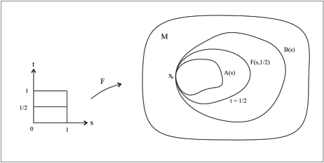
Figure 9: In the picture, we can see the representation of the homotopy between two loops.

In addition, homotopy by path is an equivalence class:

(i) Trivially, $a\approx a$ since $F\left(s,0\right)=A\left(s\right)$ is a homotopy. This is, by the way, the identity function;

(ii) Given homotopy $F$ between $a\approx b$, then $G\left(s,t\right)=F\left(s,1-t\right)$ is homotopic between $b\approx a$;

(iii) If $F$ is a homotopy $a\approx b$ and $G$ is a homotopy $b\approx c$, there is also a homotopy $H$: $a\approx c$, defined by,

$$H\left(s,t\right)=\left\{\begin{array}[c]{c}F\left(s,2t\right)\leavevmode\nobreak\ \ \ \ \ \ \ \ \ \ \ \ \text{for}\leavevmode\nobreak\ \ \ \ t\in[0,1/2]\\ G\left(s,2t-1\right)\leavevmode\nobreak\ \ \ \ \ \ \text{for}\leavevmode\nobreak\ \ \ \ t\in[1/2,1]\end{array}\right.\,.$$

The equivalence class of the loops with a base-point $x_{0}$ satisfy all the axioms of a group. It is the so-called fundamental group or the first homotopy group in $x_{0}$; it is denoted by $\pi_{1}\left(x_{0}\right)$.

We can parallel transport a vector along a particular loop to be able to measure the curvature of the region inside the loop. When we consider a continuous manifold, it is usual to use an infinitesimal loop, where we can define the local curvature, that is, curvature at a point. However, things are a bit different when we deal with a discretized manifold. In this case the curvature is associated to the deficit angle, the loop must include one or more vertexes, and the curvature measurement becomes non-local. Any loop which includes a certain vertex and it is smaller than the perimeter of a fundamental simplex always provides the same value for the deficit angle. Consequently, in a discretized manifold, the curvature is not a property associated to the infinitesimal loop itself; it is rather a property related to the homotopy group based on the vertex $m$.

In order to parallel transport a vector we need to define a connection, that is, the transport symmetry generator. In our case, the symmetry is the rotation of the vector $\mathbf{A}$ around the joint $p$. Accordingly, the generator may be taken as the rotation angle $\vec{\sigma}=\sigma\leavevmode\nobreak\ \mathbf{U}_{p}=N\leavevmode\nobreak\ \varepsilon_{p}\mathbf{U}_{p}$ of the vector $\mathbf{A}$ at the end of the transport. If the transport of $\mathbf{A}$ encompasses several vertexes, it is necessary to add the contribution from all rotation angles, in a way that the total rotation is given by

$$h=\exp\left(N\leavevmode\nobreak\ {\displaystyle\sum_{p}}\varepsilon_{p}\mathbf{U}_{p}\right)\,,$$ (26)

where $N$ is considered as approximately independent of a particular $p$-joint $(\varrho_{p}\simeq\varrho$), i.e., we take the average of the number of bones in the manifold’s $P$ joints. We call $h\mathbf{A}$ the holonomy of the vector $\mathbf{A}$ around the vertex $m$.

Holonomy is closely related to homotopy. In fact, the loops along which we parallel transport vector $\mathbf{A}$ are those in homotopy’s definition. Holonomy requires more structure, though: It demands a connection. Even with this additional element, holonomy is also an equivalence class since various distinct loops around the same vertex lead to the same value for the deficit angle. There is then an holonomy group at the loops’ base-point. This concept help us to understand the above equation for $h$: A group element can be written as an exponential of the infinitesimal generators of the transformation, just like we see in Eq. (26).

The transport of vector $\mathbf{A}$ along the simplex manifold is done along the equivalence class loops. Since those loops can be deformed in the identity loop with base-point $x_{0}$ [1], then the holonomy is the unity:

$$h=1\,.$$ (27)

Indeed, Regge advocates that two arbitrary points $P$ and $Q$ in contiguous simplexes $T^{m}$ and $T^{m+1}$ can be linked by a curve $t_{m}$, and that $t_{m}t_{m}^{-1}=u$ is the identity loop with base-point $P$ related to the joint between $T^{m}$ e $T^{m+1}$. Let’s say then that by repeating this process for all polyhedrons in the trajectory, we define the composition of curves starting at $P$ and coming back to it. This produces a loop $t_{1}t_{2}t_{3}...t_{n}$ homotopic to the identity loop $u$,

$$t_{1}t_{2}t_{3}...t_{n}\approx u\,.$$

($n$ is the number of polyhedrons in the transport. Note that a cyclic order of $1$ to $n$ was defined; this is arbitrary, but general). We arrive in the unitary holonomy in the Eq. (27) by using the identity loop as an equivalence class representative.

Substituting (27) into (26):

$$\exp\left(N\leavevmode\nobreak\ {\displaystyle\sum_{p}}\varepsilon_{p}\mathbf{U}_{p}\right)=1\,.$$

Therefore, the exponential’s argument must vanish:

$${\displaystyle\sum_{p}}\varepsilon_{p}\mathbf{U}_{p}=0\,.$$

By dualization, this is the same as:

$${\displaystyle\sum_{p}}\varepsilon_{p}U_{\mu\nu}^{p}=0\,.$$ (28)

This result followed from topological considerations. It will be key to derive Bianchi’s identity associated to the curvature on discretized manifold.

4.2.2 Relating $\varrho_{p}$ to $\varrho$

The local density of bones in the $p$-th joint, $\varrho_{p}$, cannot be constant throughout the manifold because there are regions on the manifold with higher curvature and consequently with higher concentration of polyhedrons. The rate of variation of $\varrho_{p}$ can be obtained as a function of the average bones density $\varrho$.

The density $\varrho_{p}$ is the number of bones piercing through the surface $\Sigma$ orthogonal to $\mathbf{U}^{p}$ ($\varrho_{p}$ is a superficial density). We refer the reader to Fig. 10. Let $s$ be a parameter along the bundle of bones $p$ with origin at the vertex, i.e., $s$ is along the direction of $\mathbf{U}^{p}$. The position of $\Sigma$ is determined by $s$. Now, let $C$ be a cylinder of base equals $\Sigma$ and hight $ds$.

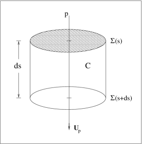
Figure 10: Infinitesimal cylinder $C$ around the sheaf $p$ of edges.

The number of bones inside the cylinder is the number of bones leaving $C$,

$$\varrho_{p}\left(s+ds\right)\leavevmode\nobreak\ \Sigma\,,$$

minus the number of bones entering $C$,

$$\varrho_{p}(s)\leavevmode\nobreak\ \Sigma\,.$$

On the other hand, the number of bones within $C$ must be the average density $\varrho$ times the volume $\Sigma\leavevmode\nobreak\ ds$ of the cylinder:

$$\varrho\left(s\right)\leavevmode\nobreak\ \Sigma\leavevmode\nobreak\ ds\,.$$

($\varrho$ is a volumetric density). Hence,

$$\varrho_{p}\left(s+ds\right)\leavevmode\nobreak\ \Sigma-\varrho_{p}(s)\leavevmode\nobreak\ \Sigma=\varrho\left(s\right)\leavevmode\nobreak\ \Sigma\leavevmode\nobreak\ ds\,,$$

i.e.,

$$\varrho=\frac{d\varrho_{p}}{ds}\,.$$ (29)

The derivative in (29) is the directional derivative along the bundle of bones, that is, along the $\mathbf{U}^{p}$ direction. In the Cartesian coordinate system, this equation reads:

$$\varrho=\frac{dx^{\mu}}{ds}\frac{d\varrho_{p}}{dx^{\mu}}=U_{p}^{\mu}\frac{d\varrho_{p}}{dx^{\mu}}=\mathbf{U}_{p}\cdot\mathbf{\nabla}\varrho_{p}\,.$$ (30)

Notice the identification $U_{p}^{\mu}=dx^{\mu}/ds$ is reasonable because $dx^{\mu}/ds$ is the “velocity vector” along the bone.

4.2.3 Calculating $B_{\lambda\alpha\beta\mu\nu}$ in the discretized manifold

Keeping in mind the results in Sections 4.2.1 and 4.2.2, let us return to the problem of finding the discrete version of the second Bianchi identity.

According to (17):

$$R_{\alpha\beta\mu\nu}=\sum\limits_{p}\varrho_{p}\varepsilon_{p}U_{\leavevmode\nobreak\ \alpha\beta}^{p}U_{\leavevmode\nobreak\ \mu\nu}^{p}\,.$$ (31)

The sum was included because the parallel transport of $\mathbf{A}$ eventually encloses many joints in the simplex manifold.

In our approximation to discretize the space into Euclidian polyhedrons, the covariant derivatives in the definition of $B_{\lambda\alpha\beta\mu\nu}$,

$$B_{\lambda\alpha\beta\mu\nu}\equiv\nabla_{\lambda}R_{\alpha\beta\mu\nu}+\nabla_{\alpha}R_{\beta\lambda\mu\nu}+\nabla_{\beta}R_{\lambda\alpha\mu\nu}\,,$$

reduce to ordinary derivatives (since there is no curvature in the polyhedrons):

$$B_{\lambda\alpha\beta\mu\nu}\equiv\partial_{\lambda}R_{\alpha\beta\mu\nu}+\partial_{\alpha}R_{\beta\lambda\mu\nu}+\partial_{\beta}R_{\lambda\alpha\mu\nu}\,.$$ (32)

Next, we show Eq. (32) vanishes, indeed.

The first step is to introduce (31) in (32) and take the derivatives there indicated. $\mathbf{U}^{p}$ is constant. The deficit angle in the $p$-joint is constant:

$$\partial_{\mu}\varepsilon_{p}=0\,.$$

Therefore,

$$B_{\lambda\alpha\beta\mu\nu}=\sum\limits_{p}\varepsilon_{p}U_{\leavevmode\nobreak\ \mu\nu}^{p}\left(U_{\leavevmode\nobreak\ \alpha\beta}^{p}\partial_{\lambda}\varrho_{p}+U_{\leavevmode\nobreak\ \beta\lambda}^{p}\partial_{\alpha}\varrho_{p}+U_{\leavevmode\nobreak\ \lambda\alpha}^{p}\partial_{\beta}\varrho_{p}\right)\,.$$ (33)

Now, we make use of the identity

$$\left(U_{\leavevmode\nobreak\ \alpha\beta}^{p}\partial_{\lambda}+U_{\leavevmode\nobreak\ \beta\lambda}^{p}\partial_{\alpha}+U_{\leavevmode\nobreak\ \lambda\alpha}^{p}\partial_{\beta}\right)=\epsilon_{\alpha\beta\lambda}\leavevmode\nobreak\ \mathbf{U}_{p}\cdot\mathbf{\nabla}$$ (34)

to write (33) as:

$$B_{\lambda\alpha\beta\mu\nu}=\sum\limits_{p}\varepsilon_{p}U_{\leavevmode\nobreak\ \mu\nu}^{p}\epsilon_{\alpha\beta\lambda}\leavevmode\nobreak\ \mathbf{U}_{p}\cdot\mathbf{\nabla}\varrho_{p}\,.$$

Next, by substituting the result (30) from the last section into this equation, we have:

$$B_{\lambda\alpha\beta\mu\nu}=\epsilon_{\alpha\beta\lambda}\leavevmode\nobreak\ \varrho\sum\limits_{p}\varepsilon_{p}U_{\mu\nu}^{p}\,.$$

Finally, Eq. (28) from Section 4.2.1, lead us to:

$$B_{\lambda\alpha\beta\mu\nu}=0\,.$$ (35)

This is the second Bianchi identity for the discretized version of gravitation.

In order to feel completely satisfied with the demonstration of (35), we should also derive (34). In fact,

$$\mathbf{U}_{p}\cdot\mathbf{\nabla} =U_{p}^{\mu}\partial_{\mu}=\frac{1}{2}\epsilon^{\alpha\beta\mu}U_{\leavevmode\nobreak\ \alpha\beta}^{p}\partial_{\mu}=$$

$$=\frac{1}{2}\left[\frac{1}{3}\left(\epsilon^{\alpha\beta\mu}+\epsilon^{\beta\mu\alpha}+\epsilon^{\mu\alpha\beta}\right)\right]U_{\leavevmode\nobreak\ \alpha\beta}^{p}\partial_{\mu}$$

by the cyclic property of $\epsilon^{\alpha\beta\mu}$ indexes. Distributing $U_{\leavevmode\nobreak\ \alpha\beta}^{p}\partial_{\mu}$ and renaming dummy indexes,

$$\mathbf{U}_{p}\cdot\mathbf{\nabla}=\frac{1}{6}\epsilon^{\alpha\beta\mu}\left[U_{\leavevmode\nobreak\ \alpha\beta}^{p}\partial_{\mu}+U_{\leavevmode\nobreak\ \mu\alpha}^{p}\partial_{\beta}+U_{\leavevmode\nobreak\ \beta\mu}^{p}\partial_{\alpha}\right]\,.$$

Hence:

$$\epsilon_{\alpha\beta\mu}\leavevmode\nobreak\ \mathbf{U}_{p}\cdot\mathbf{\nabla}=\frac{1}{6}\left(\epsilon_{\alpha\beta\mu}\epsilon^{\alpha\beta\mu}\right)\left[U_{\leavevmode\nobreak\ \alpha\beta}^{p}\partial_{\mu}+U_{\leavevmode\nobreak\ \mu\alpha}^{p}\partial_{\beta}+U_{\leavevmode\nobreak\ \beta\mu}^{p}\partial_{\alpha}\right]\,.$$

From Eq. (11):

$$\left(\epsilon_{\alpha\beta\mu}\epsilon^{\alpha\beta\mu}\right)=\left(\delta_{\leavevmode\nobreak\ \alpha}^{\alpha}\delta_{\leavevmode\nobreak\ \beta}^{\beta}-\delta_{\leavevmode\nobreak\ \beta}^{\alpha}\delta_{\leavevmode\nobreak\ \alpha}^{\beta}\right)=\left(3^{2}-\delta_{\leavevmode\nobreak\ \alpha}^{\alpha}\right)=9-3=6\,.$$

Substituting this in the above expression results in:

$$\epsilon_{\alpha\beta\mu}\leavevmode\nobreak\ \mathbf{U}_{p}\cdot\mathbf{\nabla}=U_{\leavevmode\nobreak\ \alpha\beta}^{p}\partial_{\mu}+U_{\leavevmode\nobreak\ \mu\alpha}^{p}\partial_{\beta}+U_{\leavevmode\nobreak\ \beta\mu}^{p}\partial_{\alpha}\,,$$

which is exactly the identity (34) we wanted demonstrated.

We are now ready to build the skeleton version fo Einstein field equation for gravity. This will be accomplished in the upcoming section.

5 Action Integral and Einstein Equations in Simplex Gravity

5.1 Regge’s action

The sourceless gravity field equations are found by varying Einstein-Hilbert action [5]

$$I=\frac{1}{16\pi}\int d^{4}x\leavevmode\nobreak\ \sqrt{-g}\leavevmode\nobreak\ R$$ (36)

with respect to the metric tensor $g^{\mu\nu}$. This tensor encapsulates all information about curvature: Christoffel symbols and the curvature tensor are written in terms of the metric and its derivatives. In fact,

$$\frac{\delta I}{\delta g^{\mu\nu}}=0\,,$$ (37)

leads to [2]:

$$R_{\mu\nu}-\frac{1}{2}g_{\mu\nu}R=0\,.$$ (38)

Our next task is to suggest a version of the equations above for the simplex manifold. The integral in (36) is translated to a sum over all the $p$ joints. In Section 3 we obtained the discretized version of the scalar curvature: $R=2\varrho_{p}\varepsilon_{p}$, cf. Eq. (19). What is the analogous of the measure $d^{4}x\leavevmode\nobreak\ \sqrt{-g}$? Regge suggests that the adequate measure for the discretized action $I$ is the quantity $L_{p}=L_{p}\left(\varrho_{p}\right)$ defined at the $p$-joint. In three dimensions $L_{p}$ is simply the length $l_{p}$ of the bones in the hinge. In four dimensions $L_{p}$ is actually the area of the simplexes edges at the $p$-joint. Thus,

$$\frac{1}{16\pi}\int d^{4}x\leavevmode\nobreak\ \sqrt{-g}\leavevmode\nobreak\ R\rightarrow\frac{1}{16\pi}\sum\limits_{p}L_{p}\left(2\varepsilon_{p}\right)\,,$$

where the density $\varrho_{p}$ coming from $R$ was included into the functional form of $L_{p}=L_{p}(\varrho_{p})$. The action according to Regge is, then:

$$I=\frac{1}{8\pi}\sum\limits_{p}\varepsilon_{p}L_{p}\,.$$ (39)

The measure $L_{p}$ can be written in terms of the length $l_{p}$ of the $p$-joint (according to Section 5.3 below). We also know that the length of the bones yields the same type of information about the skeleton manifold that the metric provides for the continuous manifold. For this reason, we choose to take $l_{p}$ as the variation parameter of $I$. Accordingly, the analogous of (37) is:

$$\frac{\delta I}{\delta l_{p}}=0\,,$$ (40)

which, in view of Eq. (39), reads:

$$\delta I=\frac{1}{8\pi}\sum\limits_{p}\delta\varepsilon_{p}L_{p}+\frac{1}{8\pi}\sum\limits_{p}\varepsilon_{p}\delta L_{p}\,.$$ (41)

We need another long digression (Section 5.2) to show that the first term on the right-hand side of (41) is zero. This is rather surprising since $\varepsilon_{p}$ depends on $l_{p}$. However, the effort is necessary to derive the discrete version of Einstein equations. In Section 5.3 we find $\delta L_{p}$ as a function of $l_{p}$. Finally, Regge field equations are built in Section 5.4.

5.2 Checking $\sum\limits_{p}\delta\varepsilon_{p}L_{p}=0$

Consider the following example: a triangle is a two-dimensional simplex represented by $T_{2}$. The edges of $T_{2}$ are three straight segments, which are the unidimensional simplexes, $T_{1}$. In order to assemble $T_{2}$, it was necessary to gather $2+1=3$ simplexes $T_{1}$. The fundamental simplex in three dimensions is the tetrahedron. A tetrahedron $T_{3}$ is composed of $3+1=4$ triangles $T_{2}$. This can be generalized: Let $T_{n}$ be a simplex of dimension $n$. The edges are simplexes $T_{n-1}$. It is necessary $\left(n+1\right)$ simplexes $T_{n-1}$ to generate a fundamental $T_{n}$ simplex, eventually used to discretize the manifold. Let $r$ and $s$ be the labels used to identify the edge-simplexes $T_{n-1}$, so that $r,s=0,1,2,...,\left(n+1\right)$. Fig. 11 shows a two-dimensional representation of $T_{n-1}^{r}$.

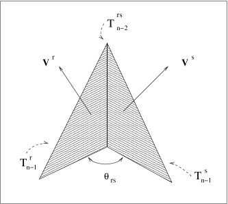
Figure 11: Two-dimensional representation of the simplexes $T_{n-1}^{r}$ and $T_{n-1}^{s}$ and their comum edge $T_{n-2}^{rs}$. The unit vectors $V_{\mu}^{r}\$and $V_{\nu}^{s}$ are normal to $T_{n-1}^{r}$ and $T_{n-1}^{s}$.

Any two contiguous simplexes $T_{n-1}^{r}$ and $T_{n-1}^{s}$ share a common edge. According to the previous discussion, the edge has the dimension $\left(n-2\right)$ and label $rs$. The edge is, then, denoted by $T_{n-2}^{rs}$. By definition, $\theta_{rs}$ is the angle in between $T_{n-1}^{r}$ and $T_{n-1}^{s}$.

Now we define unitary vectors $V_{\mu}^{r}$ and $V_{\mu}^{s}$ normal to (the “surface” of) $T_{n-1}^{r}$ and $T_{n-1}^{s}$. The index $\mu$ refers to the components of $\mathbf{V}$ in a Cartesian coordinate system defined in the manifold.

The following identities hold:

1. Unitary norm:

   $$\left\|\mathbf{V}^{r}\right\|^{2}=V_{\leavevmode\nobreak\ \mu}^{r}V_{r}^{\leavevmode\nobreak\ \mu}=1\,.$$ (42)

   (The position of the label $r$ is irrelevant; but the position is important for $\mu$, which respects Einstein’s summation convention). The same is valid for $\mathbf{V}^{s}$.

2. Dot product:

   $$\mathbf{V}^{r}\cdot\mathbf{V}^{s}=\left\|\mathbf{V}^{r}\right\|\left\|\mathbf{V}^{s}\right\|\cos\theta_{rs}\,,$$

   i.e.,

   $$V_{\leavevmode\nobreak\ \mu}^{r}V^{s\mu}=\cos\theta_{rs}\,.$$ (43)

Consider the antisymmetric tensor $\mathbf{V}^{rs}$,

$$V_{\mu\nu}^{rs}=-V_{\nu\mu}^{rs}\,,$$ (44)

inspired by the vector product definition:

$$V_{\mu\nu}^{rs}=\frac{1}{\sin\theta_{rs}}\left(V_{\leavevmode\nobreak\ \mu}^{r}V_{\leavevmode\nobreak\ \nu}^{s}-V_{\leavevmode\nobreak\ \nu}^{r}V_{\leavevmode\nobreak\ \mu}^{s}\right)\,,$$ (45)

where the factor $\left(1/\sin\theta_{rs}\right)$ may be seen as a normalization factor of $V_{\mu\nu}^{rs}$.

However, there is a fundamental difference between the definition $\mathbf{V}^{rs}$ and the cross product $\left(\mathbf{V}^{r}\times\mathbf{V}^{s}\right)$, namely the dualization process. While $\left(\mathbf{V}^{r}\times\mathbf{V}^{s}\right)$ is an axial vector, $\mathbf{V}^{rs}$ is its dual quantity. That means $\left(\mathbf{V}^{r}\times\mathbf{V}^{s}\right)$ is orthogonal to $\mathbf{V}^{r}$ and to $\mathbf{V}^{s}$, i.e. it is orthogonal to the area defined by them – see Fig. 12. On the other hand, $\mathbf{V}^{rs}$ can be understood as a quantity over the area, defining an orientation thereof.

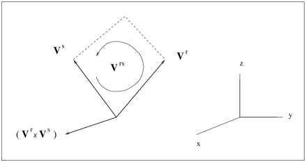
Figure 12: Pictorically, $\left(\mathbf{V}^{r}\times\mathbf{V}^{s}\right)$ is “orthogonal” to $\mathbf{V}^{rs}$.

The contraction $V_{\mu\nu}^{rs}V_{rs}^{\mu\nu}$ of the antisymmetric tensors is the following:

$$V_{\mu\nu}^{rs}V_{rs}^{\mu\nu} =\frac{1}{\sin^{2}\theta_{rs}}\left[\left(V_{\mu}^{r}V_{r}^{\mu}\right)\left(V_{\nu}^{s}V_{s}^{\nu}\right)-\left(V_{\mu}^{r}V_{r}^{\nu}\right)\left(V_{\nu}^{s}V_{s}^{\mu}\right)+\right.$$

$$\left.-\left(V_{\nu}^{r}V_{r}^{\mu}\right)\left(V_{\mu}^{s}V_{s}^{\nu}\right)+\left(V_{\nu}^{r}V_{r}^{\nu}\right)\left(V_{\mu}^{s}V_{s}^{\mu}\right)\right]\,.$$

From (42) and (43):

$$V_{\mu\nu}^{rs}V_{rs}^{\mu\nu}=\frac{1}{\sin^{2}\theta_{rs}}\left[2-2\cos^{2}\theta_{rs}\right]\,,$$

that is,

$$V_{\mu\nu}^{rs}V_{rs}^{\mu\nu}=2\leavevmode\nobreak\ .$$ (46)

Now, take the variation of (43):

$$\delta\left(V_{\leavevmode\nobreak\ \mu}^{r}V^{s\mu}\right)=\delta\left(\cos\theta_{rs}\right)\,,$$

or

$$\delta V_{\leavevmode\nobreak\ \mu}^{r}V^{s\mu}+V_{\leavevmode\nobreak\ \mu}^{r}\delta V^{s\mu}=-\sin\theta_{rs}\leavevmode\nobreak\ \delta\theta_{rs}\,,$$

or yet,

$$\delta\theta_{rs}=-\frac{1}{\sin\theta_{rs}}\left(V_{\leavevmode\nobreak\ \mu}^{r}\delta V^{s\mu}+V_{\leavevmode\nobreak\ \mu}^{s}\delta V^{r\mu}\right)\,.$$ (47)

It will be handy to rewrite this equation in terms of the object $V_{\mu\nu}^{rs}$. For this end, we contract $V_{\mu\nu}^{rs}$, Eq. (45), with $V_{r}^{\mu}$:

$$V_{\mu\nu}^{rs}V_{r}^{\mu} =\frac{1}{\sin\theta_{rs}}\left(V_{\leavevmode\nobreak\ \mu}^{r}V_{r}^{\mu}V_{\leavevmode\nobreak\ \nu}^{s}-V_{\leavevmode\nobreak\ \nu}^{r}V_{r}^{\mu}V_{\leavevmode\nobreak\ \mu}^{s}\right)=$$

$$=\frac{1}{\sin\theta_{rs}}\left(V_{\leavevmode\nobreak\ \nu}^{s}-V_{\leavevmode\nobreak\ \nu}^{r}\cos\theta_{rs}\right)\,,$$

where we have used (42) and (43) again. Next, consider the contraction with $\delta V_{r}^{\nu}$:

$$V_{\mu\nu}^{rs}V_{r}^{\mu}\delta V_{r}^{\nu}=\frac{1}{\sin\theta_{rs}}\left(V_{\leavevmode\nobreak\ \nu}^{s}\delta V_{r}^{\nu}-\cos\theta_{rs}V_{\leavevmode\nobreak\ \nu}^{r}\delta V_{r}^{\nu}\right)\,.$$ (48)

However, the last term cancels out. This follows from (42):

$$\delta\left(V_{\leavevmode\nobreak\ \mu}^{r}V_{r}^{\leavevmode\nobreak\ \mu}\right)=\delta\left(1\right)=0\,,$$

i.e.,

$$\delta V_{\leavevmode\nobreak\ \mu}^{r}V_{r}^{\leavevmode\nobreak\ \mu}+V_{\leavevmode\nobreak\ \mu}^{r}\delta V_{r}^{\leavevmode\nobreak\ \mu}=0\leavevmode\nobreak\ .$$

Raising and lowering the indexes in the first term, it results:

$$\delta V_{\leavevmode\nobreak\ \mu}^{r}V_{r}^{\leavevmode\nobreak\ \mu}=0\,,$$

as stated. Therefore, identity (48) reduces to:

$$V_{\mu\nu}^{rs}V_{r}^{\mu}\delta V_{r}^{\nu}=\frac{1}{\sin\theta_{rs}}V_{\leavevmode\nobreak\ \nu}^{s}\delta V_{r}^{\nu}\,,$$

or,

$$V_{\leavevmode\nobreak\ \nu}^{s}\delta V_{r}^{\nu}=\sin\theta_{rs}\left(V_{\mu\nu}^{rs}V_{r}^{\mu}\delta V_{r}^{\nu}\right)\,.$$ (49)

This is the second term of the expression (47) for $\delta\theta_{rs}$. The first term, $V_{\leavevmode\nobreak\ \mu}^{r}\delta V^{s\mu}$, comes from an entirely analogous process:

$$V_{\mu\nu}^{rs}V_{s}^{\mu} =\frac{1}{\sin\theta_{rs}}\left(V_{\leavevmode\nobreak\ \mu}^{r}V_{s}^{\mu}V_{\leavevmode\nobreak\ \nu}^{s}-V_{\leavevmode\nobreak\ \nu}^{r}V_{\leavevmode\nobreak\ \mu}^{s}V_{s}^{\mu}\right)=$$

$$=\frac{1}{\sin\theta_{rs}}\left(V_{\leavevmode\nobreak\ \nu}^{s}\cos\theta_{rs}-V_{\leavevmode\nobreak\ \nu}^{r}\right)\,.$$

$$V_{\mu\nu}^{rs}V_{s}^{\mu}\delta V_{s}^{\nu}=\frac{1}{\sin\theta_{rs}}\left(\cos\theta_{rs}V_{\leavevmode\nobreak\ \nu}^{s}\delta V_{s}^{\nu}-V_{\leavevmode\nobreak\ \nu}^{r}\delta V_{s}^{\nu}\right)=-\frac{1}{\sin\theta_{rs}}V_{\leavevmode\nobreak\ \nu}^{r}\delta V_{s}^{\nu}\,.$$

$$V_{\leavevmode\nobreak\ \nu}^{r}\delta V^{s\nu}=-\sin\theta_{rs}V_{\mu\nu}^{rs}V_{s}^{\mu}\delta V_{s}^{\nu}\,.$$ (50)

Substituting (49) and (50) into Eq. (47):

$$\delta\theta_{rs}=-\frac{1}{\sin\theta_{rs}}\left(-\sin\theta_{rs}V_{\mu\nu}^{rs}V_{s}^{\mu}\delta V_{s}^{\nu}+\sin\theta_{rs}V_{\mu\nu}^{rs}V_{r}^{\mu}\delta V_{r}^{\nu}\right)\,.$$

Renaming the repeated indexes in the second term and using the antisymmetry of $V_{\mu\nu}^{rs}$:

$$\delta\theta_{rs}=-V_{\mu\nu}^{rs}\left(V_{s}^{\mu}\delta V_{s}^{\nu}+V_{r}^{\nu}\delta V_{r}^{\mu}\right)\,.$$ (51)

The deficit angle $\varepsilon_{p}$ associated to the node $p$ is given in term of the sum of dihedral angles $\theta_{rs}$ on that node,

$$\varepsilon_{p}=2\pi-\sum_{\left(rs\right)}\theta_{rs}\,.$$

The change in $\varepsilon_{p}$ is, therefore, written as the function of $\delta\theta_{rs}$:

$$\delta\varepsilon_{p}=-\sum_{\left(rs\right)}\delta\theta_{rs}\,.$$

The sum of $\delta\varepsilon_{p}$ over all the $p$-joints weighted by the generalized area $L_{p}$ of the joint is:

$$\sum\limits_{p}\delta\varepsilon_{p}L_{p} =-\sum\limits_{p}\sum_{\left(rs\right)}\delta\theta_{rs}L_{rs}^{p}=$$

$$=\sum\limits_{p}\sum_{\left(rs\right)}\left(V_{s}^{\mu}\delta V_{s}^{\nu}+V_{r}^{\nu}\delta V_{r}^{\mu}\right)V_{\mu\nu}^{rs}L_{rs}^{p}\,,$$ (52)

where we have used (51). $L_{rs}^{p}$ is the contribution for the measure from each joint.

Note that the sum over the pair $\left(rs\right)$ labeling a particular edge is equivalent to a sum over the adjoint surfaces $r$ and $s$:

$$\sum_{\left(rs\right)}\rightarrow\sum_{r}\sum_{s}\text{ \ \ or \ \ }\sum_{s}\sum_{r}\,.$$ (53)

In effect, consider the pyramid vertex $\mathcal{V}$ in Fig. 13. The vertex $\mathcal{V}$ is related to the joint $p$ of interest here. The index $(rs)$ indicates, for example, the edge $\mathcal{VB}$ when we defined $\mathbf{V}^{r}$ on the face $\mathcal{VBC}$ and $\mathbf{V}^{s}$ on the face $\mathcal{VAB}$.

Figure 13: The pyramidal simplex example allows us to understand that the sum over the edges $(r,s)$ is equivalent to the sum over the adjoint faces $r$ and $s$. See Eq. (53) and discussion below it.

The sum over $(rs)$ means adding the contributions of all the edges $\mathcal{VB}$, $\mathcal{VC}$, $\mathcal{VD}$ and $\mathcal{VA}$. For that end, we subsequently place the pair $\mathbf{V}^{r}$ and $\mathbf{V}^{s}$ on different pairs of faces: First, $\mathbf{V}^{r}$ is placed on the face $\mathcal{VBC}$ and $\mathbf{V}^{s}$ is placed on the face $\mathcal{VAB}$ (Fig. 13); this counts the contribution by the edge $\mathcal{VB}$. After that, we take $\mathbf{V}^{r}$ on $\mathcal{VAB}$ and $\mathbf{V}^{s}$ on $\mathcal{VDA}$ to account for the contribution of the edge $\mathcal{VA}$; and so on. The act of changing from one edge to the next means to compute one more term in the sum over $(rs)$.

Alternatively, the summation procedure could be the following. Place $\mathbf{V}^{r}$ on the face $\mathcal{VBC}$ and place $\mathbf{V}^{s}$ on the contiguous faces: first on $\mathcal{VAB}$ (to count the edge $\mathcal{VB}$) and then on the face $\mathcal{VCD}$ (to account for $\mathcal{VC}$). That is, fix index $r$ and sum over $s$. We still need to consider the contribution of the edges $\mathcal{VD}$ and $\mathcal{VA}$. We then take $\mathbf{V}^{r}$ on $\mathcal{VDA}$ and place $\mathbf{V}^{s}$ on $\mathcal{VCD}$ (to count $\mathcal{VD}$); after that $\mathbf{V}^{s}$ is placed on $\mathcal{VAB}$ ( to account for $\mathcal{VA}$). When we changed the position of $\mathbf{V}^{r}$ we performed the summation over $r$. This completes te sum of both indexes.

This method described in the two paragraphs above are evidently equivalent: in both cases we add the contribution of all the edges in Fig. 13. This explains the prescription in Eq. (53).

After those remarks, we conclude that Eq. (52) can be cast into the form :

$$\sum\limits_{p}\delta\varepsilon_{p}L_{p}=\sum\limits_{p}\left[\sum_{s}V_{s}^{\mu}\delta V_{s}^{\nu}\sum_{r}V_{\mu\nu}^{rs}L_{rs}^{p}+\sum_{r}V_{r}^{\nu}\delta V_{r}^{\mu}\sum_{s}V_{\mu\nu}^{rs}L_{rs}^{p}\right]\,.$$ (54)

For orthogonality reasons, it is true that

$$\sum_{s}V_{\mu\nu}^{rs}L_{rs}^{p}=0\,,$$ (55)

For this reason, the right-hand side of Eq. (54) vanishes entirely:

$$\sum\limits_{p}\delta\varepsilon_{p}L_{p}=0\,,$$ (56)

as anticipated.

5.3 Evaluating $\delta L_{p}$

In four dimensions, the sheaf will not be a straight (oriented) line of length $l_{p}$. On the contrary, it will be a bidimensional surface with area $L_{p}$ (and border $l_{p}$, for example). We are interested in obtaining the area $L_{p}$ as a function of $l_{p}$ in order to establish the discrete version of the field equations for gravity in 4D.

For simplicity, let us consider the bidimensional area $L_{p}$ as the isosceles triangle of base $l_{p}$; cf. Fig. 14.

Figure 14: Isosceles triangle of sides $a$, $a$ and $l_{p}$. $\theta_{p}$ is the opposite angle to $l_{p}$, and $\alpha$ the opposite angle to $a$.

From elementary geometry, the area $L_{p}$ is

$$L_{p}=\frac{1}{2}\left(\text{base}\right)\left(\text{hight}\right)=\frac{1}{2}l_{p}h\leavevmode\nobreak\ ;$$ (57)

and the hight $h$ follows from

$$a^{2}=\left(\frac{l_{p}}{2}\right)^{2}+h^{2}\,.$$ (58)

The side $a$ is:

$$\sin\frac{\theta_{p}}{2}=\frac{\left(l_{p}/2\right)}{a}\Rightarrow a=\frac{l_{p}}{2}\frac{1}{\sin\frac{\theta_{p}}{2}}\,.$$ (59)

Substituting (59) into (58):

$$h^{2}=\left(\frac{l_{p}}{2}\right)^{2}\left(\frac{1}{\sin^{2}\frac{\theta_{p}}{2}}-1\right)\,,$$

i.e,

$$h=\frac{l_{p}}{2}\frac{\cos\frac{\theta_{p}}{2}}{\sin\frac{\theta_{p}}{2}}\leavevmode\nobreak\ .$$ (60)

Hence, the area equation (57) turns to

$$L_{p}=\left(\frac{l_{p}}{2}\right)^{2}\cot\frac{\theta_{p}}{2}\,.$$ (61)

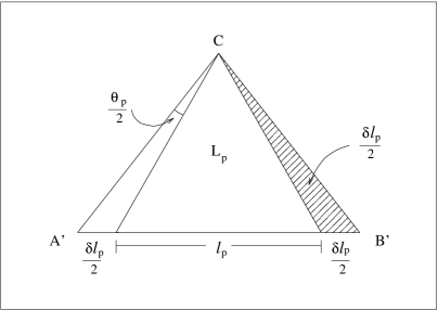
Figure 15: Variation of the area of the isosceles triangle by increment in $l_{p}$.

If we vary $l_{p}$ in a way to increment by equal quantities $\delta l_{p}/2$ both extremities of the base, the triangle remains isosceles — see Fig. 15. The opposite angle to the incremented base $l_{p}^{\prime}$,

$$l_{p}^{\prime}=\frac{\delta l_{p}}{2}+l_{p}+\frac{\delta l_{p}}{2}$$

increases to

$$\theta_{p}^{\prime}=\frac{\delta\theta_{p}}{2}+\theta_{p}+\frac{\delta\theta_{p}}{2}\,.$$

Since the post-variation triangle remains isosceles, its area $L_{p}^{\prime}=L_{p}+\delta L_{p}$ is calculated by Eq. (61):

$$L_{p}^{\prime}=\left(\frac{l_{p}^{\prime}}{2}\right)^{2}\cot\left(\frac{\theta_{p}^{\prime}}{2}\right)=\left(\frac{l_{p}+\delta l_{p}}{2}\right)^{2}\cot\left(\frac{\theta_{p}+\delta\theta_{p}}{2}\right)\,;$$

where

$$\left(l_{p}+\delta l_{p}\right)^{2}=l_{p}^{\leavevmode\nobreak\ 2}+2l_{p}\leavevmode\nobreak\ \delta l_{p}+\delta l_{p}^{\leavevmode\nobreak\ 2}\simeq l_{p}^{\leavevmode\nobreak\ 2}+2l_{p}\leavevmode\nobreak\ \delta l_{p}\,,$$

since second order increments are neglected. Moreover, expanding $\cot\theta_{p}^{\prime}$ in Taylor series about $\theta_{p}/2$ yields:

$$\cot\left(\frac{\theta_{p}+\delta\theta_{p}}{2}\right)=\cot\frac{\theta_{p}}{2}+\left.\frac{d}{d\theta_{p}}\cot\left(\frac{\theta_{p}+\delta\theta_{p}}{2}\right)\right|_{\theta_{p}/2}\frac{\delta\theta_{p}}{2}+\mathcal{O}\left(\frac{\delta\theta_{p}^{\leavevmode\nobreak\ 2}}{4}\right)\,,$$

where

$$\frac{d}{dx}\cot x=-\frac{1}{\sin^{2}x}=-\left(1-\cot^{2}x\right)\,.$$

It then follows:

$$L_{p}^{\prime}=\frac{\left(l_{p}^{\leavevmode\nobreak\ 2}+2l_{p}\delta l_{p}\right)}{4}\left[\cot\frac{\theta_{p}}{2}-\frac{1}{\sin^{2}\frac{\theta_{p}}{2}}\frac{\delta\theta_{p}}{2}\right]+\mathcal{O}\left(\delta l_{p}^{\leavevmode\nobreak\ 2},\delta\theta_{p}^{\leavevmode\nobreak\ 2}\right)\,,$$

i.e.,

$$L_{p}+\delta L_{p}=\frac{l_{p}^{\leavevmode\nobreak\ 2}}{4}\cot\frac{\theta_{p}}{2}+\frac{1}{2}l_{p}\delta l_{p}\cot\frac{\theta_{p}}{2}-\frac{1}{4}l_{p}^{\leavevmode\nobreak\ 2}\frac{1}{\sin^{2}\frac{\theta_{p}}{2}}\frac{\delta\theta_{p}}{2}+\mathcal{O}\left(\delta l_{p}^{\leavevmode\nobreak\ 2},\delta\theta_{p}^{\leavevmode\nobreak\ 2}\right)\,.$$

The first term in the right-hand side of the equation above is precisely $L_{p}$, Eq. (61). It cancels out the first term in the left-hand side. Thus,

$$\delta L_{p}\simeq\frac{1}{2}l_{p}\delta l_{p}\cot\frac{\theta_{p}}{2}-\frac{1}{4}l_{p}^{\leavevmode\nobreak\ 2}\frac{1}{\sin^{2}\frac{\theta_{p}}{2}}\frac{\delta\theta_{p}}{2}\,.$$ (62)

The term $\delta\theta_{p}$ in (62) is of the same order as $\delta l_{p}$. Fig. 16 helps us to check this out.

Figure 16: Triangle $BCB^{\prime}$ resulting from the increment $\delta l_{p}$ on the base of triangle $ABC$ of Fig. 14. The same triangle is highlighted in Fig. 15.

Based on Fig. 16, we write:

$$\sin\left(\alpha+\delta\alpha\right)=\frac{b}{\left(\delta l_{p}/2\right)}\,.$$ (63)

On the other hand, from the geometry of the original isosceles triangle in Fig. 14:

$$\alpha=\frac{\pi}{2}-\frac{\theta_{p}}{2}\,.$$

Therefore, $\delta\alpha$ reads:

$$\delta\alpha=-\frac{\delta\theta_{p}}{2}\,.$$

Consequently,

$$\sin\left(\alpha+\delta\alpha\right)=\sin\left[\frac{\pi}{2}-\frac{\left(\theta_{p}+\delta\theta_{p}\right)}{2}\right]=\cos\left(\frac{\theta_{p}+\delta\theta_{p}}{2}\right)\,.$$ (64)

Equating (63) and (64):

$$\cos\left(\frac{\theta_{p}+\delta\theta_{p}}{2}\right)=\frac{b}{\left(\delta l_{p}/2\right)}\,;$$

i.e.

$$b=\frac{\delta l_{p}}{2}\cos\left(\frac{\theta_{p}+\delta\theta_{p}}{2}\right)\,.$$ (65)

Yet another result from Fig. 16:

$$\sin\left(\frac{\delta\theta_{p}}{2}\right)=\frac{b}{a}\,.$$

Substituting the expressions (59) and (65) for $a$ and $b$:

$$\sin\left(\frac{\delta\theta_{p}}{2}\right)=\frac{\delta l_{p}}{l_{p}}\sin\frac{\theta_{p}}{2}\cos\left(\frac{\theta_{p}+\delta\theta_{p}}{2}\right)\,.$$

Now, we use the fact

$$\frac{\delta\theta_{p}}{2}\ll 1$$

to approximate

$$\sin\left(\frac{\delta\theta_{p}}{2}\right)=\frac{\delta\theta_{p}}{2}+\mathcal{O}\left(\frac{\delta\theta_{p}^{\leavevmode\nobreak\ 3}}{8}\right)$$

and

$$\cos\left(\frac{\theta_{p}+\delta\theta_{p}}{2}\right)=\cos\left(\frac{\theta_{p}}{2}\right)+\mathcal{O}\left(-\sin\frac{\theta_{p}}{2}\leavevmode\nobreak\ \frac{\delta\theta_{p}}{2}\right)\,,$$

so that

$$\frac{\delta\theta_{p}}{2}\simeq\frac{\delta l_{p}}{l_{p}}\sin\frac{\theta_{p}}{2}\cos\frac{\theta_{p}}{2}\,.$$ (66)

Substituting (66) into Eq. (62) for $\delta L_{p}$, we get:

$$\delta L_{p}\simeq\frac{1}{2}l_{p}\delta l_{p}\cot\frac{\theta_{p}}{2}-\frac{1}{4}l_{p}\delta l_{p}\frac{\cos\frac{\theta_{p}}{2}}{\sin\frac{\theta_{p}}{2}}\,.$$

Therefore, up to order-$\left(\delta l_{p}\right)^{2}$ terms, it results:

$$\delta L_{p}=\frac{1}{4}l_{p}\delta l_{p}\cot\frac{\theta_{p}}{2}\,.$$ (67)

This is the last ingredient we needed for writing the final version of Regge’s action integral.

5.4 The discretized version of Einstein equations

Substituting (56) and (67) into (41), it follows:

$$\delta I=\frac{1}{8\pi}\sum\limits_{p}\varepsilon_{p}\left(\frac{1}{4}l_{p}\delta l_{p}\cot\frac{\theta_{p}}{2}\right)\,.$$

We now adopt the approximation in which all $p$ joints in the manifold have the same length $l_{p}$ on average,

$$l_{p}\simeq l\,.$$

This is consistent with the simplicity hypothesis that is convenient to triangulate the manifold using polyhedrons as close to regular polyhedrons as possible. It is also consistent with the $L_{p}$ calculation in the previous subsection.

Accordingly, the variations with respect to $l_{p}$ should be, on average, the same for all $p$ joints. This means:

$$\delta l_{p}\simeq\delta l\,,$$

leading to

$$\frac{\delta I}{\delta l}=\frac{1}{32\pi}l\sum\limits_{p}\varepsilon_{p}\cot\frac{\theta_{p}}{2}\leavevmode\nobreak\ ,$$ (68)

since the product $l_{p}\leavevmode\nobreak\ \delta l_{p}\simeq l\leavevmode\nobreak\ \delta l$ can be taken off the sum in $p$.

The principle of minimal action manifested in Eq. (40) enforces the vanishing of Eq. (68) which leads to Einstein equations for the discretized space:

$$\sum\limits_{p}\varepsilon_{p}\cot\frac{\theta_{p}}{2}=0\,.$$ (69)

This result is analogous to (38).

6 Final Remarks

In this paper, we have meticulously studied the seminal work by Regge on the discretized version of general relativity. We have made an effort to bring the abstract and synthetic style of the original paper [1] to a more down to Earth and step-by-step approach to the subject. Regge calculus is a fundamental theoretical background to a numerical treatment of curvature and there lies the key importance of the subject.

Regge’s discretized version of gravitation has a parallel with the Quantum Chromodynamics Theory in its attempt to perform network calculations [10]. Indeed, some argue that Regge calculus would be the appropriate way to quantize gravitation, despite its limitations [11].

Regge calculus was applied to the Schwarzschild solution and to the study of Reissner-Nordström geometry [12]. The Friedmann models were also treated in the light of this method [12]. Ref. [13] builds the simplex version of the action integral for higher order gravity. The construction of the teleparallel equivalent of Regge equations in [14] is another application to gravitation. Refs. [15, 16] contain a formal approach to Regge calculus and further applications (see also references therein).

Recently, advances in computational capacity have led to a renewed interest in Regge calculus, especially after the successes obtained within Quantum Chromodynamics. This culminated in a new version of Regge’s theory called Dynamic Causal Triangulation [17].

Perhaps the most recent application of the subject of this paper is the relationship between Regge calculus and the spin networks used in Loop Quantum Gravity. In fact, it is possible to show that spin networks are a dual representation of Regge’s spacetime triangulation. For instance, in order to picture a tetrahedron as a spin network, we use a vertex to denote the volume and four links to represent the four faces. The value of the volume is given by a number in the vertex and the faces’ areas are related to four numbers (one for each link). In the quantized version, each area is described by an area operator, which is closed under the $su(2)$ algebra plus a closure relation [18]. Each vertex is expressed by a volume operator, and the spin network is the basis which simultaneously diagonalizes both operators. Regge calculus is very important for Loop Quantum Gravity to obtain the necessary classical limit.

It is our hope this paper will facilitate the interested reader to enter the field.

Acknowledments

The authors are grateful to Ruben Aldrovandi, José G. Pereira, Bruto M. Pimentel and Teófilo Vargas from IFT-Unesp (Brazil) for references and insightful discussions.

References

- [1] T. Regge, General Relativity without Coordinates, Nuovo Cimento, XIX, 3, 559 (1961).
- [2] C. W. Misner, K. S. Thorne and J. A. Wheeler, Gravitation, Princeton University Press (2017).
- [3] M. Nakahara, Geometry, Topology and Physics, 2nd ed.,Taylor & Francis, Boca Raton (2003).
- [4] R. Aldrovandi and J. G. Pereira, An Introduction to Geometrical Physics, World Scientific, Singapore (1995).
- [5] V. Sabbata and M. Gasperini, Introduction to Gravitation, World Scientific, Singapore (1985).
- [6] A. Ozakin, A. Yavari, Affine development of closed curves in Weitzenböck manifolds and the Burgers vector of dislocation mechanics, Mathematics and Mechanics of Solids 19 (2012) 299-307.
- [7] J. B. Marion and S. T. Thornton, Classical Dynamics of Particles and Systems, 4th edition, Saunders College Publishing, 1995.
- [8] B. Felsager, Geometry, Particles and Fields, Springer, New York, (1997).
- [9] R. Gilmore, Lie Groups, Lie Algebras, and Some of Their Applications, Dover, New York (2006).
- [10] J. Smit, Introduction to Quantum Fields on a Lattice, Cambridge University Press, Cambridge (2002).
- [11] G. Immirzi, Quantum Gravity and Regge Calculus, Nucl. Phys. Proc. Suppl. 57 (1997) 65-72.
- [12] J. A. Wheeler, Relativity, Groups and Topology, edited by B. DeWitt and C. DeWitt, Gordon and Breach, New York (1964) 463.
- [13] H. W. Hamber, Critical Phenomena Random Systems, Gauge Theories, edited by K. Osterwalder and R. Stora, Elsevier (1986), 375.
- [14] J. G. Pereira and T. Vargas, Regge Calculus in Teleparallel Gravity, Classical and Quantum Gravity 19 (2002) 4807-4816.
- [15] J. R. McDonald and W. A. Miller, Coupling non-gravitational fields with simplicial spacetimes, Classical and Quantum Gravity 27 (2010) 095011.
- [16] W. A. Miller, J. R. McDonald, P. M. Alsing, D. X. Gu and S.-T. Yau, Simplicial Ricci flow, Communications in Mathematical Physics 2 (2014) 579-608.
- [17] R Loll, The emergence of spacetime or quantum gravity on your desktop, Classical and Quantum Gravity 25 (2008) 114006; J. Ambjorn, J. Jurkiewicz, R. Loll, Quantum gravity as sum over spacetimes, arXiv:0906.3947 (2009).
- [18] C. Rovelli and F. Vidotto, Covariant Loop Quantum Gravity: An Elementary Introduction to Quantum Gravity and Spin Foam Theory, Cambridge University Press (2014).