Some complexity measures in confined isotropic harmonic oscillator

Abstract

Various well-known statistical measures like López-Ruiz, Mancini, Calbet (LMC) and Fisher-Shannon complexity have been explored for confined isotropic harmonic oscillator (CHO) in composite position ($r$) and momentum ($p$) spaces. To get a deeper insight about CHO, a more generalized form of these quantities with Rényi entropy ($R$) is invoked here. The importance of scaling parameter in the exponential part is also investigated. $R$ is estimated considering order of entropic moments $\alpha,\beta$ as $(\frac{2}{3},3)$ in $r$ and $p$ spaces respectively. Explicit results of these measures with respect to variation of confinement radius $r_{c}$ is provided systematically for first eight energy states, namely, $1s,~{}1p,~{}1d,~{}2s,~{}1f,~{}2p,~{}1g$ and $2d$. Detailed analysis of these complexity measures provides many hitherto unreported interesting features.

PACS: 03.65-w, 03.65Ca, 03.65Ta, 03.65.Ge, 03.67-a.

Keywords: LMC complexity, Fisher-Shannon complexity, Rényi entropy, Shannon entropy, Confined isotropic harmonic oscillator.

I introduction

Quantum particles undergo dramatic changes in their chemical and physical properties under extreme pressure. Such situations may be achieved by shifting their spatial boundary from infinity to finite region michels37 . The effect of boundary condition and boundary limit on various observable properties such as energy spectrum, transition frequency, transition probability, polarizability, chemical reactivity, ionization potential etc., were studied in considerable detail in last ten years sabin2009 ; sen2014electronic . These systems have their comprehensive and potential application in nano-science and technology, condensed matter physics, semiconductor physics, quantum dot, quantum wells and quantum wires, etc sabin2009 ; sen2014electronic .

From the beginning of this century there has been a thriving interest in exploring statistical quantities namely, Fisher information ($I$), Onicescu energy ($E$), Shannon entropy ($S$) and Rényi entropy ($R$) as signifier of certain chemical, physical properties of a quantum system. In the same direction, complexity, another topical concept, is directly concerned to aforesaid measures and illustrates their combined effect. A global definition of complexity has not yet been possible. But it may be treated as a demonstrator of pattern, structure or correlation related with the distribution function in a given system. It depends on the scale of inspection, and comprises an important area of investigation with contemporary interest in chaotic systems, spatial patterns, language, multi-electronic systems, molecular or DNA analysis, social science, astrophysics and cosmology rosso03 ; shalizi04 ; chatzisavvas05 ; bouvrie11 etc.

A quantum harmonic oscillator is a complex system; circumscribing its oscillation within an impenetrable region makes it even more impressive according to a complex world goldenfeld99 ; sen12 . Complexity, in a system, is introduced by disrupting certain rules of symmetry. A system possesses finite complexity when it is either in a state having less than some maximal order or not at a state of equilibrium. In a nutshell, it vanishes at two limiting cases, viz., when a system is (i) completely ordered (maximum distance from equilibrium) or (ii) at equilibrium (maximum disorder) sen12 . Overall it provides a characteristic idea of distribution in a system and is deliberated as a general descriptor of structure and correlation. In literature several definitions are available; some of them are Shiner, Davidson, Landsberg (SDL) landsberg84 ; landsberg98 ; shiner99 , López-Ruiz, Mancini, Calbet (LMC) shape ($C_{LMC}$) lopezruiz95 ; anteneodo96 ; catalan02 ; sanchez05 , Fisher-Shannon ($C_{IS}$) romera04 ; sen07 ; angulo08 , Cramér-Rao dehesa06 ; angulo08 ; antolin09 or Generalized Rényi-like complexity calbet01 ; martin06 ; romera08 ; lopezruiz09 , generalized relative complexity measures romera11 etc.

Without any loss of generality, the statistical measure of complexity, may be defined as a product of ordered and disordered parameters in the following form,

$$C_{LMC}=H.D,$$ (1)

where H represents the information content and D narrates an idea of concentration of spatial distribution. For a normalized continuous distribution $p(\mathrm{\mathbf{r}})$ these two quantities were expressed lopezruiz95 in the form $H=-k\int p(\mathrm{\mathbf{r}})\mathrm{log}\ p(\mathrm{\mathbf{r}})\mathrm{d}\mathrm{\mathbf{r}}$ ($k$ is a positive constant) and $D=\int p^{2}(\mathrm{\mathbf{r}})\mathrm{d}\mathrm{\mathbf{r}}$. But, this definition of $C_{LMC}$ was criticized feldman98 due to its inability to satisfy necessary conditions such as reaching minimal values for both extremely ordered and disordered limits, invariance under scaling, translation and replication. Therefore, this model was modified lopez05 , giving rise to the expression,

$$C_{\emph{LMC}}=D.{e^{S}}.$$ (2)

Here, $S$ quantifies the information of a given system and has the mathematical form $-\int p(\mathrm{\mathbf{r}})\mathrm{log}\ p(\mathrm{\mathbf{r}})\mathrm{d}\mathrm{\mathbf{r}}$. Principally $C_{\emph{LMC}}$ quantifies the interaction between intrinsic information hidden in a system, and measure of a probabilistic distribution amongst its observed parts. It has potential application in several fields like detection of periodic, quasi-periodic, linear stochastic, chaotic dynamics lopezruiz95 ; yamano04 ; yamano04a and in quantum phase transition nagy12 ; romera14 .

In information theory $E$ measures information content of a system. It sets off to minimum at equilibrium. Hence $E$ signifies a descriptor of order. Whereas information entropies like $S,R$, become maximum at equilibrium, thereby implying disorder. Complexity quantifies the extent of countervail between order and disorder. In many instances, $E$ is replaced by $I$. So far in the literature $S$ has been primarily used as disorder parameter. $C_{IS}$ is another measure, attained by changing the pre-exponential global factor in $C_{LMC}$ by a local factor like $I$. It unites global and local characters while conserving the characteristics of complexity. Effectiveness of $C_{IS}$ can be reviewed by looking at numerous literature available for both free and confined atomic systems, including atomic shell structure, ionization process angulo08 ; sen07 ; antolin09 ; angulo08a ; szabo08 etc. Recently a more generalized version was also designed that uses $R$ in place of $S$, in $C_{LMC}$ and $C_{IS}$ sen12 . Later, a scaling factor ($b$) was invoked in exponential part.

About a decade ago, both $C_{LMC}$ and $C_{IS}$ were explored in the context of Bohr-like states of free isotropic harmonic oscillator (IHO) in $r,p$ spaces sanudo08 . However, in confined environment LMC complexity has been investigated only for ground state of some model systems, like, CHO, confined h-atom, particle in spherical box and confined Helium atom romera09 ; nagy09 . Very recently, the present authors have pursued similar calculations for confined hydrogen atom majumder17 and found that, parameter $b$ plays a key role in interpreting the property of a system. In this endeavor, our objective is to explore four different types of complexity emerging out of two order ($I,E$) and two disorder ($S,R$) parameters, in conjugate spaces, as functions of confinement radius ($r_{c}$). We take into account two $b$ values available in literature sen12 , and these are ($\frac{2}{3}$ for $C_{IS}$, 1 for $C_{LMC}$). All calculations were carried out using exact wave functions of CHO in $r$ space. The $p$-space wave function is computed by applying numerical Fourier transform of $r$-space counterpart. In the end, representative calculation are done for eight low-lying states viz., $1s,~{}1p,~{}1d,~{}2s,~{}1f,~{}2p,~{}1g$ and $2d$. Presentation of the article is as follows. Section II gives a brief outline of the theoretical method used; Sec. III presents a thorough discussion on our results, while we conclude with a few remarks in Sec. IV.

II Methodology

The time-independent, non-relativistic wave function for a CHO system, in $r$ space can be written as,

$$\Psi_{n,l,m}(\mathrm{\mathbf{r}})=\psi_{n,l}(r)\ Y_{l,m}(\Omega),$$ (3)

with $r$ and $\Omega$ representing radial distance and solid angle successively. Here $\psi_{n,l}(r)$ denote the radial part and $Y_{l,m}(\Omega)$ identifies spherical harmonics. The latter has following common form in both $r$ and $p$ spaces ($P_{l}^{m}(\cos\theta)$ denotes usual associated Legendre polynomial),

$$Y_{l,m}({\Omega})=\Theta_{l,m}(\theta)\ \Phi_{m}(\phi)=(-1)^{m}\sqrt{\frac{2l+1}{4\pi}\frac{(l-m)!}{(l+m)!}}\ P_{l}^{m}(\cos\theta)\ e^{-im\phi}.$$ (4)

The relevant radial Schrödinger equation under the influence of confinement is,

$$\left[-\frac{1}{2}\ \frac{d^{2}}{dr^{2}}+\frac{l(l+1)}{2r^{2}}+v(r)+v_{c}(r)\right]\psi_{n,l}(r)=\mathcal{E}_{n,l}\ \psi_{n,l}(r),$$ (5)

where $v(r)=\frac{1}{2}\omega^{2}r^{2}$ and $\omega$ is the oscillator frequency. Our required confinement effect is induced by invoking the following form of potential: $v_{c}(r)=+\infty$ for $r>r_{c}$, and $0$ for $r\leq r_{c}$, where $r_{c}$ denotes radius of confinement.

Exact generalized radial wave function for a CHO is mathematically expressed as montgomery07 ,

$$\psi_{n_{r},l}(r)=N_{n_{r},l}\ r^{l}\ _{1}F_{1}\left[\frac{1}{2}\left(l+\frac{3}{2}-\frac{\mathcal{E}_{n_{r},l}}{\omega}\right),(l+\frac{3}{2}),\omega r^{2}\right]e^{-\frac{\omega}{2}r^{2}}.$$ (6)

Here, $N_{n,l}$ represents normalization constant and $\mathcal{E}_{n,l}$ corresponds to the energy of a given state distinguished by quantum numbers $n,l$, whereas ${}_{1}F_{1}\left[a,b,r\right]$ represents confluent hypergeometric function. Allowed energies are obtained by applying the boundary condition $\psi_{n,\ell}(0)=\psi_{n,\ell}\ (r_{c})=0$ (except for $l=0$ states, only $\psi_{n,\ell}\ (r_{c})=0$ ). In this work, generalized pseudospectral (GPS) method was employed to calculate $\mathcal{E}_{n,l}$ of these states. This method has provided very accurate results for various model and real systems including atoms, molecules, some of which could be found in the references roy04 ; sen06 ; roy15 . This is very well documented and therefore omitted here.

The $p$-space wave function is obtained from Fourier transform of $r$-space counterpart,

$$\psi_{n,l}(p) = \frac{1}{(2\pi)^{\frac{3}{2}}}\ \int_{0}^{r_{c}}\int_{0}^{\pi}\int_{0}^{2\pi}\psi_{n,l}(r)\ \Theta(\theta)\Phi(\phi)\ e^{ipr\cos\theta}r^{2}\sin\theta\ \mathrm{d}r\mathrm{d}\theta\mathrm{d}\phi$$ (7)

$$= \frac{1}{2\pi}\sqrt{\frac{2l+1}{2}}\int_{0}^{r_{c}}\int_{0}^{\pi}\psi_{n,l}(r)\ P_{l}^{0}(\cos\theta)\ e^{ipr\cos\theta}\ r^{2}\sin\theta\ \mathrm{d}r\mathrm{d}\theta.$$

Here $\psi(p)$ is not normalized and needs to be normalized. Integrating over $\theta$ and $\phi$ yields,

$$\psi_{n,l}(p)=(-i)^{l}\int_{0}^{r_{c}}\ \frac{\psi_{n,l}(r)}{p}\ f(r,p)\mathrm{d}r.$$ (8)

$f(r,p)$ depends only on $l$ quantum number. It can be expressed in terms of Cos and Sin series. More details about $f(r,p)$ could be found in mukherjee18 .

The normalized position and momentum electron densities are expressed as,

$$\rho(\mathrm{\mathbf{r}})=|\psi_{n,l,m}(\mathrm{\mathbf{r}})|^{2},\ \ \ \ \ \ \Pi(\mathrm{\mathbf{p}})=|\psi_{n,l,m}(\mathrm{\mathbf{p}})|^{2}.$$ (9)

Without any loss of generality, let us express complexity in a generalized mathematical form as $C=Ae^{b.B}$. The order ($A$) and disorder parameters ($B$) may comprise of ($E,I$) and ($R,S$) respectively. With this in mind, we are interested in the following four quantities,

$$C_{ER} =Ee^{bR},\ \ \ \ \ \ \ \ C_{IR}=Ie^{bR},\ \ \ \ \ \ \ C_{ES} =Ee^{bS},\ \ \ \ \ \ \ \ C_{IS}=Ie^{bS}.$$ (10)

Shannon entropy of a continuous density distribution is written as (‘t’ stands for total),

$$S_{\mathrm{\mathbf{r}}} =-\int_{{\mathcal{R}}^{3}}\rho(\mathrm{\mathbf{r}})\ \ln[\rho(\mathrm{\mathbf{r}})]\ \mathrm{d}\mathrm{\mathbf{r}};\ \ \ S_{\mathrm{\mathbf{p}}} =-\int_{{\mathcal{R}}^{3}}\Pi(\mathrm{\mathbf{p}})\ \ln[\Pi(\mathrm{\mathbf{p}})]\ \mathrm{d}\mathrm{\mathbf{p}};\ \ \ S_{t} =S_{\mathrm{\mathbf{r}}}+S_{\mathrm{\mathbf{p}}}.$$ (11)

Similarly, Rényi entropy of order $\alpha(\neq 1)$ is obtained by taking logarithm of $\alpha$ and $\beta$-order entropic moments in respective spaces sen12 ,

$$R_{\mathrm{\mathbf{r}}}^{\alpha}=\frac{1}{1-\alpha}\ln\left(\int_{{\mathcal{R}}^{3}}\rho^{\alpha}(\mathrm{\mathbf{r}})\mathrm{d}\mathrm{\mathbf{r}}\right);\ \ \ R_{\mathrm{\mathbf{p}}}^{\beta}=\frac{1}{1-\beta}\ln\left[\int_{{\mathcal{R}}^{3}}\Pi^{\beta}(\mathrm{\mathbf{p}})\mathrm{d}\mathrm{\mathbf{p}}\right];\ \ \ R_{t}=R_{\mathrm{\mathbf{r}}}^{\alpha}+R_{\mathrm{\mathbf{p}}}^{\beta}.$$ (12)

where,

$$\frac{1}{\alpha}+\frac{1}{\beta}=2$$

$I_{\mathrm{\mathbf{r}}}$, $I_{\mathrm{\mathbf{p}}}$ for a particle in a central potential may be expressed as romera05 ,

$$I_{\mathrm{\mathbf{r}}} =4\langle p^{2}\rangle-2(2l+1)|m|\langle r^{-2}\rangle;\ \ \ I_{\mathrm{\mathbf{p}}} =4\langle r^{2}\rangle-2(2l+1)|m|\langle p^{-2}\rangle;\ \ \ I_{t}=I_{\mathrm{\mathbf{r}}}I_{\mathrm{\mathbf{p}}}.$$ (13)

Finally, $E$ is given by the following expressions in conjugate space sen12 ,

$$E_{\mathrm{\mathbf{r}}} =\int_{{\mathcal{R}}^{3}}\rho^{2}(\mathrm{\mathbf{r}})\mathrm{d}\mathrm{\mathbf{r}};\ \ \ E_{\mathrm{\mathbf{p}}} =\int_{{\mathcal{R}}^{3}}\Pi^{2}(\mathrm{\mathbf{p}})\mathrm{d}\mathrm{\mathbf{p}};\ \ \ E_{t}=E_{\mathrm{\mathbf{r}}}E_{\mathrm{\mathbf{p}}}.$$ (14)

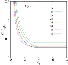
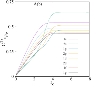
Figure 1: Variation of $C_{E_{\mathrm{\mathbf{r}}}S_{\mathrm{\mathbf{r}}}}^{(1)},~{}C_{E_{\mathrm{\mathbf{p}}}S_{\mathrm{\mathbf{p}}}}^{(1)}$ (bottom row A) and $C_{E_{\mathrm{\mathbf{r}}}S_{\mathrm{\mathbf{r}}}}^{(2)},~{}C_{E_{\mathrm{\mathbf{p}}}S_{\mathrm{\mathbf{p}}}}^{(2)}$ (top row B) in CHO with $r_{c}$ for $1s,1p,1d,2s,1f,2p,1g,2d$ states. See text for details.

Table 1: $C_{E_{\mathrm{\mathbf{r}}}S_{\mathrm{\mathbf{r}}}}^{(1)},~{}C_{E_{\mathrm{\mathbf{p}}}S_{\mathrm{\mathbf{p}}}}^{(1)}$ and $C_{E_{t}S_{t}}^{(2)}$ for $1s,~{}2s,~{}1p,~{}1d$ states in CHO at various $r_{c}$.

$r_{c}$	$C_{E_{\mathrm{\mathbf{r}}}S_{\mathrm{\mathbf{r}}}}^{(1)}$	$C_{E_{\mathrm{\mathbf{p}}}S_{\mathrm{\mathbf{p}}}}^{(1)}$	$C_{E_{t}S_{t}}^{(1)}$	$C_{E_{\mathrm{\mathbf{r}}}S_{\mathrm{\mathbf{r}}}}^{(1)}$	$C_{E_{\mathrm{\mathbf{p}}}S_{\mathrm{\mathbf{p}}}}^{(1)}$	$C_{E_{t}S_{t}}^{(1)}$
$1s$				$2s$
0.1	10.544267	0.02093	0.22073	19.769038	0.00985	0.19491
0.2	5.272192	0.04186	0.22074	9.8845272	0.01972	0.19499
0.5	2.1098387	0.10464	0.22079	3.9539382	0.04933	0.19504
0.8	1.3220786	0.16721	0.22106	2.4716592	0.07894	0.19513
1.0	1.0623420	0.20854	0.22154	1.9779193	0.09871	0.19525
2.5	0.5453416	0.46594	0.25409	0.7991488	0.27391	0.21889
5.0	0.5422182	0.54221	0.29399	0.6472847	0.64698	0.41878
7.0	0.5422182865	0.5422182865	0.2940006701	0.6472880855	0.6472825716	0.4189782966
$1p$				$1d$
0.1	11.363226	0.01746	0.19849	12.302938	0.01561	0.19216
0.2	5.6816369	0.03493	0.19850	6.1514809	0.03123	0.19217
0.5	2.2730425	0.08733	0.19850	2.4607796	0.07809	0.19216
0.8	1.4220367	0.13961	0.19853	1.5386569	0.12487	0.19213
1.0	1.1395261	0.17426	0.19857	1.2318435	0.15593	0.19208
2.5	0.5143143	0.40130	0.20639	0.5232749	0.36665	0.19186
5.0	0.4869827	0.48699	0.23715	0.4628145	0.46285	0.21421
7.0	0.4869829166	0.4869829186	0.237152362	0.4628158714	0.4628158704	0.2141985303

III Result and Discussion

At the onset it is convenient to point out a few points about this report. The net information measures in conjugate $r$ and $p$ space may be separated into radial and angular segments. In a given space, the results provided correspond to net measures including the angular contributions. One can transform the IHO to a CHO by pressing the radial boundary of former from infinity to a finite region. This change in radial environment does not affect the angular boundary conditions. Therefore, angular part of the information measures in unconfined and confined systems remain unaltered in both spaces. Further as we are solely focused in radial confinement, this will also not influence the characteristics of a given measure as one changes $r_{c}$. Throughout this report, magnetic quantum number $m$ remains fixed to $0$. All the discussed measures of Eq. (10) have been explored with change of $r_{c}$, choosing two different and widely used values of $b$ ($1,\frac{2}{3}$). Note that, for $b=1$, $C_{ES}^{(2)}$ modifies to $C_{LMC}$; similarly $C_{IS}^{(1)}$ coincides with $C_{IS}$ at $b=\frac{2}{3}$. In order to simplify the discussion, a few words may be devoted to the notation followed. A uniform symbol $C_{order_{s},disorder_{s}}^{b}$ is used; where the two subscripts refer to two order ($E,I$) and disorder ($S,R$) parameters. Another subscript $s$ is used to specify the space; viz., $r,p$ or $t$ (total). Two scaling parameters $b=\frac{2}{3},1$ are identified with superscripts (1), (2). These measures are offered systematically for $1s,~{}1p,~{}1d,~{}2s,~{}1f,~{}2p,~{}1g$ and $2d$ states in conjugate spaces, with $r_{c}$ varying in the range of 0.1-8.0 a.u. Also it is important to point out that, here levels are denoted by $n_{r}+1$ and $l$ values roy08 . Therefore, as an example, $n_{r}=0,l=1$ signify $1p$ state, and $n_{r}$ relates to $n$ as $n=2n_{r}+l$.

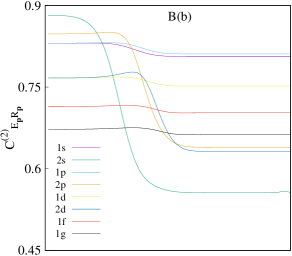
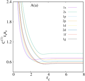
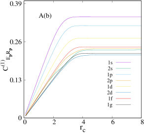
Figure 2: Changes in $C_{E_{\mathrm{\mathbf{r}}}R_{\mathrm{\mathbf{r}}}}^{(1)},~{}C_{E_{\mathrm{\mathbf{p}}}R_{\mathrm{\mathbf{p}}}}^{(1)}$ (bottom row A) and $C_{E_{\mathrm{\mathbf{r}}}R_{\mathrm{\mathbf{r}}}}^{(2)},~{}C_{E_{\mathrm{\mathbf{p}}}R_{\mathrm{\mathbf{p}}}}^{(2)}$ (top row B) in CHO with $r_{c}$ for $1s,1p,1d,2s,1f,2p,1g,2d$ states. For more details, see text.

Table 2: $C_{E_{\mathrm{\mathbf{r}}}R_{\mathrm{\mathbf{r}}}}^{(1)},~{}C_{E_{\mathrm{\mathbf{p}}}R_{\mathrm{\mathbf{p}}}}^{(1)}$ and $C_{E_{t}R_{t}}^{(1)}$ for $1s,~{}2s,~{}1p,~{}1d$ states in CHO at various $r_{c}$.

$r_{c}$	$C_{E_{\mathrm{\mathbf{r}}}R_{\mathrm{\mathbf{r}}}}^{(1)}$	$C_{E_{\mathrm{\mathbf{p}}}R_{\mathrm{\mathbf{p}}}}^{(1)}$	$C_{E_{t}R_{t}}^{(1)}$	$C_{E_{\mathrm{\mathbf{r}}}R_{\mathrm{\mathbf{r}}}}^{(1)}$	$C_{E_{\mathrm{\mathbf{p}}}R_{\mathrm{\mathbf{p}}}}^{(1)}$	$C_{E_{t}R_{t}}^{(1)}$
$1s$				$2s$
0.1	12.011965	0.01401	0.16830	25.481700	0.00761	0.19405
0.2	6.0060677	0.02802	0.16830	12.740847	0.01523	0.19415
0.5	2.4038079	0.07004	0.16838	5.0962894	0.03810	0.19417
0.8	1.5073076	0.11199	0.16881	3.1849974	0.06091	0.19401
1.0	1.2125775	0.13981	0.16953	2.5477258	0.07602	0.19369
2.5	0.6661575	0.31636	0.21074	1.0079698	0.16895	0.17030
5.0	0.7153170	0.34549	0.24713	0.8597424	0.23246	0.19985
7.0	0.7153219525	0.3454938391	0.2471393275	0.8599102013	0.2324933318	0.1999233878
$1p$				$1d$
0.1	13.160407	0.01162	0.15295	14.410589	0.00931	0.13429
0.2	6.5802381	0.02324	0.15296	7.2053113	0.01863	0.13430
0.5	2.6326593	0.05811	0.15298	2.8823989	0.04659	0.13431
0.8	1.6474274	0.09294	0.15312	1.8024800	0.07454	0.13435
1.0	1.3207023	0.11610	0.15334	1.4433285	0.09314	0.13443
2.5	0.6151214	0.27465	0.16894	0.6225095	0.22540	0.14031
5.0	0.6339254	0.31520	0.19981	0.5985573	0.27230	0.16299
7.0	0.6339446874	0.3152046743	0.1998223287	0.5986224459	0.2723045747	0.1630076305

At first, in the bottom row (panels A(a)-A(b)) of Fig. 1, $C_{E_{\mathrm{\mathbf{r}}}S_{\mathrm{\mathbf{r}}}}^{(1)},~{}C_{E_{\mathrm{\mathbf{p}}}S_{\mathrm{\mathbf{p}}}}^{(1)}$ are plotted against $r_{c}$ for all the eight states. Similarly, plots for $C_{E_{\mathrm{\mathbf{r}}}S_{\mathrm{\mathbf{r}}}}^{(2)},~{}C_{E_{\mathrm{\mathbf{p}}}S_{\mathrm{\mathbf{p}}}}^{(2)}$ are shown in panels B(a) and B(b) respectively. The lower panels clearly suggest that, $C_{E_{\mathrm{\mathbf{r}}}S_{\mathrm{\mathbf{r}}}}^{(1)}$ decreases and $C_{E_{\mathrm{\mathbf{p}}}S_{\mathrm{\mathbf{p}}}}^{(1)}$ increases with rise of $r_{c}$ before reaching a threshold corresponding to the IHO. The decrease of $C_{E_{\mathrm{\mathbf{r}}}R_{\mathrm{\mathbf{r}}}}^{(1)}$ with $r_{c}$ points to its inclination towards equilibrium. Next, panel A(a) reveals that at a fixed $l$, $C_{E_{\mathrm{\mathbf{r}}}S_{\mathrm{\mathbf{r}}}}^{(1)}$ progresses with $n$. Conversely, at a particular $n$, it reduces with growth of $l$. But panel A(b) does not imprint such patterns for $C_{E_{\mathrm{\mathbf{p}}}S_{\mathrm{\mathbf{p}}}}^{(1)}$. Panel A(c) in Figure S1 of Supplementary Material (SM) presents that $C_{E_{t}S_{t}}^{(1)}$ enhances with advancement of $r_{c}$. Now, panels B(a), B(b) delineate the variation of $C_{E_{\mathrm{\mathbf{r}}}S_{\mathrm{\mathbf{r}}}}^{(2)},~{}C_{E_{\mathrm{\mathbf{p}}}S_{\mathrm{\mathbf{p}}}}^{(2)}$ with change of $r_{c}$. One sees that, $C_{E_{\mathrm{\mathbf{r}}}S_{\mathrm{\mathbf{r}}}}^{(2)}$ advances with growth of $r_{c}$ indicating that this is more prone towards order. On the other hand, at first $C_{E_{\mathrm{\mathbf{p}}}S_{\mathrm{\mathbf{p}}}}^{(2)}$ decreases with $r_{c}$, attains a minimum and finally coalesces to IHO. The ordering of $C_{E_{\mathrm{\mathbf{r}}}S_{\mathrm{\mathbf{r}}}}^{(2)}$ regarding $n,~{}l$ quantum numbers is akin to $C_{E_{\mathrm{\mathbf{r}}}S_{\mathrm{\mathbf{r}}}}^{(1)}$. It is noticed that, after a certain $r_{c}$ ($\gtrapprox 3$), both $C_{E_{\mathrm{\mathbf{r}}}S_{\mathrm{\mathbf{r}}}}^{(2)},~{}C_{E_{\mathrm{\mathbf{p}}}S_{\mathrm{\mathbf{p}}}}^{(2)}$ show analogous nature (increase to reach their respective limiting value). Panel B(c) in Fig. S1 in SM portrays the increase of $C_{E_{t}S_{t}}^{(2)}$ with $r_{c}$. By comparing these two sets of complexity measure, namely $C^{(1)}_{ES}$ (in A(a)-A(c)) and $C^{(2)}_{ES}$ (in B(a)-B(c)), it is evident that, $C_{E_{\mathrm{\mathbf{r}}}S_{\mathrm{\mathbf{r}}}}^{(1)}$ and $~{}C_{E_{\mathrm{\mathbf{p}}}S_{\mathrm{\mathbf{p}}}}^{(1)}$ complement each other better (as former decreases and later increases with $r_{c}$) than the other set. Hence, we have presented $C_{E_{\mathrm{\mathbf{r}}}S_{\mathrm{\mathbf{r}}}}^{(1)},~{}C_{E_{\mathrm{\mathbf{p}}}S_{\mathrm{\mathbf{p}}}}^{(1)}$ and $C_{E_{t}S_{t}}^{(1)}$ at some selected $r_{c}$ values in Table I, for $1s,~{}2s,~{}1p,~{}1d$. While for $2p,~{}2d,~{}1f,~{}1g$ states these are produced in Table S1 of SM. These data consolidate the inference drawn from Figs. 1 and S1. We also see that when CHO approaches to IHO, $C_{E_{\mathrm{\mathbf{r}}}S_{\mathrm{\mathbf{r}}}}^{(1)}$ becomes equal to $~{}C_{E_{\mathrm{\mathbf{p}}}S_{\mathrm{\mathbf{p}}}}^{(1)}$. None of these results could be directly compared with literature data, as no such works have been published before, to the best of our knowledge.

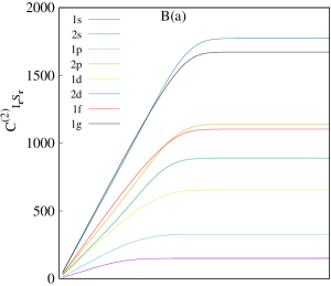
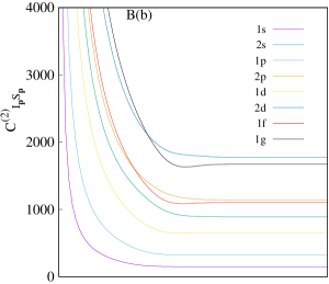
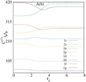
Figure 3: Variation of $C_{I_{\mathrm{\mathbf{r}}}S_{\mathrm{\mathbf{r}}}}^{(1)},~{}C_{I_{\mathrm{\mathbf{p}}}S_{\mathrm{\mathbf{p}}}}^{(1)}$ (bottom row A) $C_{I_{\mathrm{\mathbf{r}}}S_{\mathrm{\mathbf{r}}}}^{(2)},~{}C_{I_{\mathrm{\mathbf{p}}}S_{\mathrm{\mathbf{p}}}}^{(2)}$ (top row B) in CHO with $r_{c}$ for $1s,1p,1d,2s,1f,2p,1g,2d$ states. Consult text for more details.

Table 3: $C_{I_{\mathrm{\mathbf{r}}}S_{\mathrm{\mathbf{r}}}}^{(2)},~{}C_{I_{\mathrm{\mathbf{p}}}S_{\mathrm{\mathbf{p}}}}^{(2)}$ and $C_{I_{t}S_{t}}^{(2)}$ for $1s,~{}2s,~{}1p,~{}1d$ states in CHO at various $r_{c}$.

$r_{c}$	$C_{I_{\mathrm{\mathbf{r}}}S_{\mathrm{\mathbf{r}}}}^{(2)}$	$C_{I_{\mathrm{\mathbf{p}}}S_{\mathrm{\mathbf{p}}}}^{(2)}$	$C_{I_{t}S_{t}}^{(2)}$	$C_{I_{\mathrm{\mathbf{r}}}S_{\mathrm{\mathbf{r}}}}^{(2)}$	$C_{I_{\mathrm{\mathbf{p}}}S_{\mathrm{\mathbf{p}}}}^{(2)}$	$C_{I_{t}S_{t}}^{(2)}$
$1s$				$2s$
0.1	7.758205	4303.15991	33384.80018	25.056165	29216.5721	732055.2573
0.2	15.516171	2151.56736	33384.08737	50.112519	14608.3337	732060.4179
0.5	38.766040	860.42282	33355.18588	125.300544	5844.1079	732269.9114
0.8	61.804468	537.04703	33191.90621	200.655774	3655.3318	733463.4393
1.0	76.791106	428.68905	32919.50741	251.188685	2928.0196	735485.4165
2.5	145.231258	167.01717	24256.11393	663.377452	1216.9057	807267.8370
5.0	149.733084	149.73309	22419.99774	888.731009	888.9964	790078.7475
7.0	149.733087619267	149.73308721	22419.99746802	888.738383	888.7381	789855.7135
$1p$				$1d$
0.1	13.589616	10065.70616	136789.08528	23.086162	21178.15365	488922.29249
0.2	27.179055	5032.83116	136787.59609	46.172182	10589.04165	488919.15916
0.5	67.929622	2012.77692	136727.17589	115.415992	4235.04577	488792.00959
0.8	108.523492	1256.72638	136384.33569	184.533851	2644.87901	488069.71221
1.0	135.307764	1003.69056	135807.12614	230.387985	2113.17739	486850.68272
2.5	293.849512	382.32570	112346.22278	535.936973	802.82774	430265.07166
5.0	327.026856	327.02367	106945.52430	653.074539	653.04527	426487.24482
7.0	327.027007440	327.0270080	106946.6637782	653.077279415428	653.077279	426509.932617

Similarly, bottom row of Fig. 2 interprets the behavior of $C_{E_{\mathrm{\mathbf{r}}}R_{\mathrm{\mathbf{r}}}}^{(1)},~{}C_{E_{\mathrm{\mathbf{p}}}R_{\mathrm{\mathbf{p}}}}^{(1)}$ with $r_{c}$ for the same states of Fig. 1. Panel A(a) reveals that, $C_{E_{\mathrm{\mathbf{r}}}R_{\mathrm{\mathbf{r}}}}^{(1)}$ diminishes with growth of $r_{c}$, then attains a minimum and finally converges to respective IHO result. This minimum gets flatter with progress of both $n,~{}l$. Here also $C_{E_{\mathrm{\mathbf{r}}}R_{\mathrm{\mathbf{r}}}}^{(1)}$ shows analogous trend to what is noticed for $C_{E_{\mathrm{\mathbf{r}}}S_{\mathrm{\mathbf{r}}}}^{(1)}$, viz., (i) at a fixed $n$, both measures in $r$-space decline with growth of $l$ (ii) at a particular $l$, they accelerate with $n$ (iii) like $C_{E_{\mathrm{\mathbf{r}}}S_{\mathrm{\mathbf{r}}}}^{(1)}$, $C_{E_{\mathrm{\mathbf{r}}}R_{\mathrm{\mathbf{r}}}}^{(1)}$ is more inclined towards disorder. From panel A(b) it is also vivid that, like $C_{E_{\mathrm{\mathbf{p}}}S_{\mathrm{\mathbf{p}}}}^{(1)}$, $C_{E_{\mathrm{\mathbf{p}}}R_{\mathrm{\mathbf{p}}}}^{(1)}$ progress with growth of $r_{c}$. Additionally, at a definite $l$, $C_{E_{\mathrm{\mathbf{p}}}R_{\mathrm{\mathbf{p}}}}^{(1)}$ falls off with $n$. At a given $n$, it also reduces as $l$ advances. The relevant total measures are displayed in panel A(c) of Fig. S2 of SM, where prominent minima are seen for $s$ states. As usual, $C_{E_{t}R_{t}}^{(1)}$ finally merge to IHO case. Panels B(a), B(b) in top row of Fig. 2 exhibit variations of $C_{E_{\mathrm{\mathbf{r}}}R_{\mathrm{\mathbf{r}}}}^{(2)},~{}C_{E_{\mathrm{\mathbf{p}}}R_{\mathrm{\mathbf{p}}}}^{(2)}$ with $r_{c}$. At smaller $r_{c}$ region ($\lessapprox 3$), they both change very slowly. At around $r_{c}=3$, $C_{E_{\mathrm{\mathbf{r}}}R_{\mathrm{\mathbf{r}}}}^{(2)}$ jumps and $C_{E_{\mathrm{\mathbf{p}}}R_{\mathrm{\mathbf{p}}}}^{(2)}$ drops to reach the IHO limit. For both $C_{E_{\mathrm{\mathbf{r}}}R_{\mathrm{\mathbf{r}}}}^{(2)}$ and $C_{E_{\mathrm{\mathbf{p}}}R_{\mathrm{\mathbf{p}}}}^{(2)}$ absolute values of the slope of the curve enhance as $n$ grows (fixed $l$) and decrease with growth of $l$ (fixed $n$). The dependence of $C_{E_{\mathrm{\mathbf{r}}}R_{\mathrm{\mathbf{r}}}}^{(2)}$ on $n,~{}l$ is similar to $C_{E_{\mathrm{\mathbf{r}}}R_{\mathrm{\mathbf{r}}}}^{(1)}$. Panel B(c) of Fig. S2 in SM imprints the alteration of $C_{E_{t}R_{t}}^{(2)}$ with $r_{c}$ varying from 0-8. Once again one may conclude that, out of $C^{(1)}_{ER}$ and $C^{(2)}_{ER}$, the former offers a more clearer knowledge about CHO, which justifies the quantities produced in Table II, namely, $C_{E_{\mathrm{\mathbf{r}}}R_{\mathrm{\mathbf{r}}}}^{(1)}$, $C_{E_{\mathrm{\mathbf{p}}}R_{\mathrm{\mathbf{p}}}}^{(1)}$ and $C_{E_{t}R_{t}}^{(1)}$. These are given for $1s,~{}1p,~{}2s,~{}1d$ states at eight suitably chosen $r_{c}$, whereas Table S2 reports the same for $2p,~{}1f,~{}2d,~{}1g$ states. These results support the conclusions drawn from Figs. 2 and S2. Moreover it is also apparent that, there appears a minimum in $C_{E_{\mathrm{\mathbf{r}}}R_{\mathrm{\mathbf{r}}}}^{(1)}$ for all states. Similar to previous table, in this case also no literature values could be quoted. Additionally, $C_{E_{\mathrm{\mathbf{p}}}R_{\mathrm{\mathbf{p}}}}^{(1)}$ shows more lucid trend than $C_{E_{\mathrm{\mathbf{p}}}S_{\mathrm{\mathbf{p}}}}^{(1)}$ with respect to dependence of quantum numbers $n,~{}l$. Hence, in practice $C^{(1)}_{ER}$ may possibly be considered a better measure of complexity than $C^{(1)}_{ES}$.

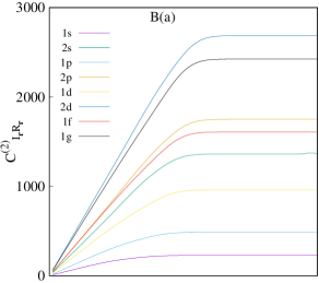
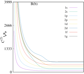
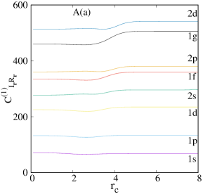
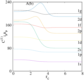
Figure 4: Plots of $C_{I_{\mathrm{\mathbf{r}}}R_{\mathrm{\mathbf{r}}}}^{(1)},~{}C_{I_{\mathrm{\mathbf{p}}}R_{\mathrm{\mathbf{p}}}}^{(1)}$ (bottom row A) and $C_{I_{\mathrm{\mathbf{r}}}R_{\mathrm{\mathbf{r}}}}^{(2)},~{}C_{I_{\mathrm{\mathbf{p}}}R_{\mathrm{\mathbf{p}}}}^{(2)}$ (top row B) in CHO with $r_{c}$ for $1s,1p,1d,2s,1f,2p,1g,2d$ states. For further details, see text.

In Fig. 3, lower {A(a), A(b)} and upper {B(a), B(b)} panels depict the alteration of $\{C_{I_{\mathrm{\mathbf{r}}}S_{\mathrm{\mathbf{r}}}}^{(1)},~{}C_{I_{\mathrm{\mathbf{p}}}S_{\mathrm{\mathbf{p}}}}^{(1)}\}$ and $\{C_{I_{\mathrm{\mathbf{r}}}S_{\mathrm{\mathbf{r}}}}^{(2)},~{}C_{I_{\mathrm{\mathbf{p}}}S_{\mathrm{\mathbf{p}}}}^{(2)}\}$ with rise in $r_{c}$ for all the states mentioned above. Nature of variation of $\{C_{I_{\mathrm{\mathbf{r}}}S_{\mathrm{\mathbf{r}}}}^{(1)},~{}C_{I_{\mathrm{\mathbf{p}}}S_{\mathrm{\mathbf{p}}}}^{(1)}\}$ with $r_{c}$ changes from state to state. From lower panels it is gathered that, at a fixed $n$, both $C_{I_{\mathrm{\mathbf{r}}}S_{\mathrm{\mathbf{r}}}}^{(1)}$ and $C_{I_{\mathrm{\mathbf{p}}}S_{\mathrm{\mathbf{p}}}}^{(1)}$ elevate with $l$. Similarly from panel A(c) in Fig. S3 of SM one can infer that, at a certain $n$, $C_{I_{t}S_{t}}^{(1)}$ increases with growth of $l$. On the other hand, the top panels B(a) and B(b) portray that, for these states $C_{I_{\mathrm{\mathbf{r}}}S_{\mathrm{\mathbf{r}}}}^{(2)}$ and $C_{I_{\mathrm{\mathbf{p}}}S_{\mathrm{\mathbf{p}}}}^{(2)}$ progress and regress with growth in $r_{c}$ and finally approach to respective IHO values. Like the previous cases, panel B(c) in Fig. S3 shows the plot of $C_{I_{t}S_{t}}^{(2)}$ versus $r_{c}$. From panels {B(a), B(b)} one observes that, at a particular $n$ both $C_{I_{\mathrm{\mathbf{r}}}S_{\mathrm{\mathbf{r}}}}^{(2)}$, $C_{I_{\mathrm{\mathbf{p}}}S_{\mathrm{\mathbf{p}}}}^{(2)}$ increase with advancement in $l$. Also, at a certain $l$, they enhance with improvement of $n$. A careful study of Figs. 3 and S3 express that, in case of CHO, $\{C_{I_{\mathrm{\mathbf{r}}}S_{\mathrm{\mathbf{r}}}}^{(2)},~{}C_{I_{\mathrm{\mathbf{p}}}S_{\mathrm{\mathbf{p}}}}^{(2)},~{}C_{I_{t}S_{t}}^{(2)}\}$ offer more transparent pattern than $\{C_{I_{\mathrm{\mathbf{r}}}S_{\mathrm{\mathbf{r}}}}^{(1)},~{}C_{I_{\mathrm{\mathbf{p}}}S_{\mathrm{\mathbf{p}}}}^{(1)},~{}C_{I_{t}S_{t}}^{(1)}\}$. So, in order to get a quantitative idea, $\{C_{I_{\mathrm{\mathbf{r}}}S_{\mathrm{\mathbf{r}}}}^{(2)},~{}C_{I_{\mathrm{\mathbf{p}}}S_{\mathrm{\mathbf{p}}}}^{(2)},~{}C_{I_{t}S_{t}}^{(2)}\}$ values at eight different $r_{c}$’s are provided in Tables III ($1s,~{}1p,~{}2s,~{}1d$) and S3 ($2p,~{}2d,~{}1f,~{}1g$). Again no results are available in literature.

Table 4: $C_{I_{\mathrm{\mathbf{r}}}R_{\mathrm{\mathbf{r}}}}^{(2)},~{}C_{I_{\mathrm{\mathbf{p}}}R_{\mathrm{\mathbf{p}}}}^{(2)}$ and $C_{I_{t}R_{t}}^{(2)}$ for $1s,~{}2s,~{}1p,~{}1d$ states in CHO at various $r_{c}$.

$r_{c}$	$C_{I_{\mathrm{\mathbf{r}}}R_{\mathrm{\mathbf{r}}}}^{(2)}$	$C_{I_{\mathrm{\mathbf{p}}}R_{\mathrm{\mathbf{p}}}}^{(2)}$	$C_{I_{t}R_{t}}^{(2)}$	$C_{I_{\mathrm{\mathbf{r}}}R_{\mathrm{\mathbf{r}}}}^{(2)}$	$C_{I_{\mathrm{\mathbf{p}}}R_{\mathrm{\mathbf{p}}}}^{(2)}$	$C_{I_{t}R_{t}}^{(2)}$
$1s$				$2s$
0.1	9.433173	2356.25770	22226.98694	36.667294	19837.6528	727393.0643
0.2	18.866136	1178.12662	22226.69794	73.334753	9918.7949	727392.3819
0.5	47.144086	471.21450	22214.97745	183.353522	3967.0032	727364.0186
0.8	75.237916	294.38160	22148.65828	293.516420	2477.4726	727178.9180
1.0	93.643707	235.33582	22037.71925	367.211469	1979.1660	726772.4766
2.5	196.075111	93.44035	18321.32860	939.702768	589.5390	553991.4457
5.0	226.884302	76.15910	17279.30538	1360.441254	191.4695	260483.1381
7.0	226.88661187	76.1582577	17279.28906	1360.840385	191.307601	260358.110977
$1p$				$1d$
0.1	16.937866	5462.96222	92530.92231	29.265843	9760.87960	285660.37271
0.2	33.875565	2731.47795	92530.35998	58.531547	4880.43593	285659.46552
0.5	84.672004	1092.53992	92507.54481	146.314712	1952.11162	285622.65198
0.8	135.321527	682.65619	92378.07852	233.974746	1219.84752	285413.51636
1.0	168.827692	545.88248	92160.08039	292.195994	975.57961	285060.45712
2.5	384.346677	216.47518	83201.51983	695.405048	386.96541	269097.70008
5.0	485.702587	170.28809	82709.36712	960.529605	294.68695	283055.54874
7.0	485.72457911	170.2950413	82716.48726	960.6865379473	294.7369698	283149.8391222

Finally, in Fig. 4 the bottom (A(a),A(b)) and top (B(a)-B(b)) panels provide the behavioral pattern in our last complexity measure, viz., $C_{I_{\mathrm{\mathbf{r}}}R_{\mathrm{\mathbf{r}}}}^{(1)},~{}C_{I_{\mathrm{\mathbf{p}}}R_{\mathrm{\mathbf{p}}}}^{(1)}$ and $C_{I_{\mathrm{\mathbf{r}}}R_{\mathrm{\mathbf{r}}}}^{(2)},~{}C_{I_{\mathrm{\mathbf{p}}}R_{\mathrm{\mathbf{p}}}}^{(2)}$ with variations in $r_{c}$. Panel A(a) reveals that, $C_{I_{\mathrm{\mathbf{r}}}R_{\mathrm{\mathbf{r}}}}^{(1)}$ progresses slowly with $r_{c}$ to attain the IHO values. At a suitable $n$ this quantity advances with $l$. In a parallel manner, at a constant $l$, $C_{I_{\mathrm{\mathbf{r}}}R_{\mathrm{\mathbf{r}}}}^{(1)}$ accumulates with $n$. Besides this, panel A(b) shows that, for circular states ($1s,~{}1p,~{}1d,~{}1f,~{}1g$) $C_{I_{\mathrm{\mathbf{p}}}R_{\mathrm{\mathbf{p}}}}^{(1)}$ diminishes with progression in $r_{c}$. But for states having one radial node ($2s,~{}2p,~{}2d$) there appears a maximum in $C_{I_{\mathrm{\mathbf{p}}}R_{\mathrm{\mathbf{p}}}}^{(1)}$. This maximum gets right shifted with increase in $l$. Now, panel A(c) of Fig. S4 implies that, the dependence of $C_{I_{t}R_{t}}^{(1)}$ on $r_{c}$ changes state-wise. Panels B(a), B(b) promptly portray that, $C_{I_{\mathrm{\mathbf{r}}}R_{\mathrm{\mathbf{r}}}}^{(2)},~{}C_{I_{\mathrm{\mathbf{p}}}R_{\mathrm{\mathbf{p}}}}^{(2)}$, accelerate and decelerate respectively with growth of $r_{c}$. Further, at a fixed $n$, both $C_{I_{\mathrm{\mathbf{r}}}R_{\mathrm{\mathbf{r}}}}^{(2)}$, $~{}C_{I_{\mathrm{\mathbf{p}}}R_{\mathrm{\mathbf{p}}}}^{(2)}$ enhance with emergence of $l$. Finally, panel B(c) of Fig. S4 in SM displays the trend of $C_{I_{t}R_{t}}^{(2)}$ with improvement of $r_{c}$. A closer investigation of Figs. 4 and S4 conveys that, $C_{I_{\mathrm{\mathbf{r}}}R_{\mathrm{\mathbf{r}}}}^{(2)},~{}C_{I_{\mathrm{\mathbf{p}}}R_{\mathrm{\mathbf{p}}}}^{(2)},~{}C_{I_{t}R_{t}}^{(2)}$ characterizes CHO better than $C_{I_{\mathrm{\mathbf{r}}}R_{\mathrm{\mathbf{r}}}}^{(1)},~{}C_{I_{\mathrm{\mathbf{p}}}R_{\mathrm{\mathbf{p}}}}^{(1)},~{}C_{I_{t}R_{t}}^{(1)}$. Thus, former three measures are given in Tables IV and S4, at some appropriately chosen $r_{c}$ for which no direct comparison could be made. It is hoped that, this study would be useful in future and inspires further work.

IV Future and outlook

Four different complexity measures namely $C_{ES},~{}C_{IS},~{}C_{ER},~{}C_{IR}$ are investigated for some low-lying states of CHO in composite $r$ and $p$ spaces, keeping $m$ fixed at zero. We have performed the calculations using a global quantity ($E$) and a local quantity ($I$). Both these may be used as measure of $order$ in a system. All these results are reported here for the first time. Sensitivity of such measures depends on the nature of the particular quantum system under investigation. It is found that, $C^{(1)}_{ES},~{}C^{(1)}_{ER}$ offer more explicit explanation than $C^{(2)}_{ES},~{}C^{(2)}_{ER}$ about a given system. On the other side, $C^{(2)}_{IS},~{}C^{(2)}_{IR}$ infer the behavior of CHO more efficiently compared to $C^{(1)}_{IS},~{}C^{(1)}_{IR}$. Hence, considering the nature of complexity measures, it is worthwhile to determine the appropriate value of $b$. Accurate results for $C^{(1)}_{ES},C^{(1)}_{ER},C^{(2)}_{IS},C^{(2)}_{IR}$ are provided for first eight states of CHO. Further, an investigation of all these quantities in the realm of Rydberg states under different kinds of soft confined environment may be worthwhile pursuing.

V Acknowledgement

Financial support from DST SERB, New Delhi, India (sanction order: EMR/2014/000838) is gratefully acknowledged. NM thanks DST SERB, New Delhi, India, for a National-post-doctoral fellowship (sanction order: PDF/2016/000014/CS).

References

- (1) A. Michels, J. de Boer and A. Bijl, Physica 4, 981 (1937).
- (2) J. R. Sabin, E. Brändas and S. A. Cruz (Eds.), The Theory of Confined Quantum Systems, Parts I and II, Advances in Quantum Chemistry, Vols. 57 and 58 (Academic Press, Cambridge, Massachusetts,2009).
- (3) K. D. Sen (Ed.), Electronic Structure of Quantum Confined Atoms and Molecules, (Springer, Switzerland, 2014).
- (4) O. A. Rosso, M. T. Martin and A. Plastino, Physica A 320, 497 (2003).
- (5) C. R. Shalizi, K. L. Shalizi and R. Haslinger, Phys. Rev. Lett. 93, 118701 (2004).
- (6) K. Ch. Chatzisavvas, Ch. C. Moustakidis and C. P. Panos, J. Chem. Phys. 123, 174111 (2005).
- (7) P. A. Bouvrie, J. C. Angulo and J. S. Dehesa, Physica A 390, 2215 (2011).
- (8) N. Goldenfeld and L. P. Kadanoff, Science 284, 87 (1999).
- (9) K. D. Sen (Ed.), Statistical Complexity: Applications in Electronic Structure, (Springer, Berlin, Germany, 2012).
- (10) P. T. Landsberg, Phys. Lett. A 102, 171 (1984).
- (11) P. T. Landsberg and J. S. Shiner, Phys. Lett. A 245, 228 (1998).
- (12) J. S. Shiner, M. Davison and P. T. Landsberg, Phys. Rev. E 59, 1459 (1999).
- (13) R. López-Ruiz, H. L. Mancini and X. Calbet, Phys. Lett. A 209, 321 (1995).
- (14) C. Anteneodo and A. R. Plastino, Phys. Lett. A 223, 348 (1996).
- (15) R. G. Catalán, J. Garay and R. López-Ruiz, Phys. Rev. E 66, 011102 (2002).
- (16) J. R. Sánchez and R. López-Ruiz, Physica A 355, 633 (2005).
- (17) E. Romera and J. S. Dehesa, J. Chem. Phys. 120, 8906 (2004).
- (18) K. D. Sen, J. Antolín and J. C. Angulo, Phys. Rev. A 76, 032502 (2007).
- (19) J. C. Angulo, J. Antolín and K. D. Sen, Phys. Lett. A 372, 670 (2008).
- (20) J. S. Dehesa, P. Sánchez-Moreno and R. J. Yáñez, J. Comput. Appl. Math. 186, 523 (2006).
- (21) J. Antolín and J. C. Angulo, Int. J. Quant. Chem. 109, 586 (2009).
- (22) X. Calbet, R. López-Ruiz, Phys. Rev. E 63, 066116 (2001).
- (23) M. T. Martin, A. Plastino and A. O. Rosso, Physica A 369, 439 (2006).
- (24) E. Romera and Á. Nagy, Phys. Lett. A 372, 6823 (2008).
- (25) R. López-Ruiz, Á. Nagy, E. Romera and J. Sañudo, J. Math. Phys. 50, 123528 (2009).
- (26) E. Romera, K. D. Sen and Á. Nagy, J. Stat. Mech. 2011, P09016 (2011).
- (27) D. P. Feldman and J. P. Crutchfield, Phys. Lett. A 238, 244 (1998).
- (28) R. López-Ruiz, Biophys. Chem. 115, 215 (2005).
- (29) T. Yamano, J. Math. Phys. 45, 1974 (2004).
- (30) T. Yamano, Physica A 340, 131 (2004).
- (31) Á. Nagy and E. Romera, Physica A 391, 3650 (2012).
- (32) E. Romera, M. Calixto and Á. Nagy, J. Mol. Model. 20, 2237 (2014).
- (33) J. C. Angulo and J. Antolín, J. Chem. Phys. 128, 164109 (2008).
- (34) J. B. Szabó, K. D. Sen and Á. Nagy, Phys. Lett. A 372, 2428 (2008).
- (35) J. Sañudo and R. López-Ruiz, J. Phys. A 41, 265303 (2008).
- (36) Á. Nagy, K. D. Sen and H. E. Montgomery Jr., Phys. Lett. A 373, 2552 (2009).
- (37) E. Romera, R. López-Ruiz, J. Sañudo and Á. Nagy, Int. Rev. Phys. 3, 207 (2009).
- (38) S. Majumdar, N. Mukherjee and A. K. Roy, Chem. Phys. Lett. 687, 322, (2017).
- (39) H. E. Montgomery Jr., N. A. Aquino and K. D. Sen, Int. J. Quant. Chem. 107, 798 (2007).
- (40) A. K. Roy, J. Phys. G 30, 269 (2004).
- (41) K. D. Sen and A. K. Roy, Phys. Lett. A 357, 112 (2006).
- (42) A. K. Roy, Int. J. Quant. Chem. 115, 937 (2015); ibid., 116, 953 (2016).
- (43) N. Mukherjee and A. K. Roy, Int. J. Quant. Chem. e25596 (2018).
- (44) E. Romera, P. Sánchez-Moreno and J. S. Dehesa, Chem. Phys. Lett. 414, 468, (2005).
- (45) A. K. Roy, A. F. Jalbout and E. I. Proynov, Int. J. Quant. Chem. 108, 827 (2008).