Floquet engineering to exotic topological phases in systems of cold atoms
Abstract
Topological phases with a widely tunable number of edge modes have been extensively studied as a typical class of exotic states of matter with potentially important applications. Although several models have been shown to support such phases, they are not easy to realize in solid-state systems due to the complexity of various intervening factors. Inspired by the realization of synthetic spin-orbit coupling in a cold-atom system [Z. Wu et al., Science 354, 83 (2016)], we propose a periodic quenching scheme to realize large-topological-number phases with multiple edge modes in optical lattices. Via introducing the periodic quenching to the Raman lattice, it is found that a large number of edge modes can be induced in a controllable manner from the static topologically trivial system. Our result provides an experimentally accessible method to artificially synthesize and manipulate exotic topological phases with large topological numbers and multiple edge modes.
I Introduction
Since the discovery of the quantum Hall effect Thouless et al. (1982), exotic phases with topologically protected edge modes have attracted extensive attention in the past decades. The study in this field has enriched our understanding of topological nature of matters, and has led to the discovery of topological insulators Hasan and Kane (2010); Fu et al. (2007), topological superconductors Qi and Zhang (2011), Weyl semimetals Burkov and Balents (2011); Wan et al. (2011); Lv et al. (2015); Burkov et al. (2011); Lu et al. (2015); Xu et al. (2015), and photonic topological insulators Lu et al. (2014); Khanikaev et al. (2012); Slobozhanyuk et al. (2016); Maczewsky et al. (2017); Ozawa et al. (2019). An intriguing direction in this field is to seek for novel phases with large topological numbers. Such phases can provide more edge modes, which are expected to improve performance of certain devices by lowering the contact resistance in quantum anomalous Hall insulators Wang et al. (2013); Fang et al. (2014). They may also be used to realize reflectionless waveguides, combiners, and one-way photonic circuits in photonic devices Haldane and Raghu (2008); Skirlo et al. (2014, 2015). Although theoretical studies suggest several models that support such phases Skirlo et al. (2015); Goldman (2009), an experimental realization is not easy due to the complication of interplay among various types of degrees of freedom in solid-state systems.
Another possible route toward realizing topological phases is to periodically drive a traditional insulator to become a so-called Floquet topological insulators. The band structure of a given system can be drastically altered by periodic driving, such as an electromagnetic field Yao et al. (2007); Oka and Aoki (2009); Lindner et al. (2011); Kitagawa et al. (2011); Dóra et al. (2012); Inoue and Tanaka (2010) and periodic quenching Foster et al. (2013); Sacramento (2014); Bhattacharya et al. (2017); Fulga and Maksymenko (2016); Caio et al. (2015); Foster et al. (2014); Wang et al. (2017a); Zhou and Gong (2018); Klinovaja et al. (2016); Ünal et al. (2019); Pérez-González et al. (2019). In addition, periodic driving can also induce an equivalent long-range hopping which is crucial for certain exotic topological phases Mikami et al. (2016); Xiong et al. (2016). However, the implementation of these schemes is usually difficult in veritable materials. Recently, the realization of synthetic spin-orbit coupling via Raman transition has paved the route toward quantum emulation of topological systems in ultracold atomic gases Lin et al. (2011); Huang et al. (2016); Wu et al. (2016); Chen et al. (2018). Owing to the high controllability therein, cold atoms confined in traps and optical lattices provide a promising platform to synthesize and study topological matters, as demonstrated in various examples Eckardt (2017); Jünemann et al. (2017); Tran et al. (2017); Gross and Bloch (2017); Potirniche et al. (2017); Wang et al. (2017b); Price et al. (2017); Zhang et al. (2018); Cooper et al. (2019); Peter et al. (2015).
In this work, we investigate exotic phases with large topological numbers of the cold-atom systems confined in an optical lattice with synthetic spin-orbit coupling implemented by a Raman lattice. By periodically driving the offset phase between the Raman lattice and the optical lattice, we find that a widely tunable number of edge modes can be generated at ease in both the one- (1D) and two-dimensional (2D) cases. A criterion to determine the change of topological numbers when changing the driving parameters across the phase boundaries is established. As the experimental techniques of Raman lattice and periodic driving both have been successfully demonstrated in cold-atom systems, our proposal can be readily implemented.
II Floquet topological phases
We are interested in topological phase transitions in a time-periodic system with period . The Floquet theorem promises a complete basis from . Here and play the same role as the stationary states and eigen energies in static systems. They are called quasistationary states and quasienergies Sambe (1973); Chen et al. (2015). It is in the quasienergy spectrum that the topological properties of our periodic system is defined. The Floquet equation is equivalent to , where is the evolution operator with being the time-ordering operator. Thus, defines an effective static system that shares the same (quasi)energies with the periodic system. Then one can use the well-developed tool of topological phase transition in static systems to study periodic systems via .
To facilitate understanding of the underlying physics, we consider a Hamiltonian with the parameter in periodically quenched between two chosen and within the respective time duration and Jiang et al. (2011). Applying the Floquet theorem, we obtain Xiong et al. (2016) with the Bloch vector and
| (1) | |||||
| (2) | |||||
where and is the unit vector of . The topological properties of the system are crucially dependent on the presence or absence of the chiral symmetry, which is tunable by the periodic quenching Asbóth et al. (2014); Rodriguez-Vega and Seradjeh (2018); Xu et al. (2018). For example, the chiral symmetry is present if , which is obviously satisfied by when the -component of is absent. Thus the chiral symmetry is present if the Bloch vector has only two components. Supplying a good way to recover the chiral symmetry by eliminating a component of , the periodic quenching can be used to generate topological phases in different classes, e.g., multiple Majorana edge modes in Kitaev chains Tong et al. (2013). Note that if both of have the identical chiral symmetry and , a unitary transformation can convert into the one with the same chiral symmetry (see Appendix A).
Different from the static case, the edge modes for the periodically driven system can occur at both of the quasienergies and . It means that two topological invariants which separately count the edge modes at and are generally needed Asbóth et al. (2014). The topological phase transition is associated with the closing and reopening of the quasienergy bands. We obtain from Eq. (2) that the bands close when
| (3) | |||
| (4) |
with quasienergy being zero () for even (odd) , or
| (5) |
As the sufficient condition for judging the phase transition, Eqs. (3)-(5) offer a guideline to design the quenching scheme to generate various topological phases at will.
III Cold-atom system
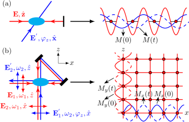
Inspired by the experimental realization of synthetic spin-orbit coupling in cold-atom systems Lin et al. (2011); Huang et al. (2016); Wu et al. (2016); Chen et al. (2018), we consider setups in dimensions () as depicted in Fig. 1. The Hamiltonian is
| (6) |
where is the Zeeman splitting, is the optical lattice, and is the Raman lattice. is formed by a standing wave for , and by two standing waves and for of frequency . is formed by the combined actions of the aforementioned standing waves and additional running waves, which take the form for , and and for of frequency . Here, is the initial phase and with being the optical path difference. The lattice potentials and together induce a two-photon Raman transition between the near-degenerate ground states mediated by the excited state Liu et al. (2014). By adiabatically eliminating , we have with for , and for with and when .
Expanding Eq. (6) in the basis of -band Wannier functions , we obtain
| (7) | |||||
where denotes that the summation is subjected to nearest neighbors, , and Wu et al. (2016). Owing to the periodicity of the potential, we have for both the 1D and 2D cases. Also, one can verify that for , and and for Liu et al. (2013); Pan et al. (2015). Defining and making the Fourier transform with being the total site number, we obtain with and the summation over the first Brillouin zone (BZ). The Bloch vectors read
| (8) | |||||
| (9) | |||||
where the lattice constant has been set to one. The particle-hole symmetry is naturally kept. Because has two components, the static Hamiltonian possesses the chiral symmetry with and belongs to the symmetry class BDI Chiu et al. (2016); Kitagawa et al. (2010). The topological properties are characterized by the winding number with the Bloch states of the 1D Hamiltonian. When , the system has and hosts one pair of edge modes Li et al. (2014). The topological property for is described by the Chern number for the lower band, where is the chirality and is the set of band-touching points for excluding the component Sticlet et al. (2012). The system has and one pair of edge states when Liu et al. (2014).
To realize the phases with larger topological numbers and more edge modes than the static cases, we consider an experimentally accessible periodic-quenching protocol
| (10) |
It is achievable by either tuning the Raman lattice depth or changing the phase of the running waves.
IV Numerical results
IV.1 Periodic quenching in 1D case
Choosing and by pairwisely changing between and , we find that the component of is zero. Thus keeps the chiral symmetry and still belongs to the symmetry class BDI. From Eqs. (3), (4), and (8), we have the conditions for the bands closing as follows.
Case I: . If this is satisfied for some at a certain , then for any subsequent one always has a that holds the condition. Thus the bands keep closed at the zero quasienergy and no phase transition occur.
Case II: . Equation (3) requires . Further with Eq. (4), we obtain . Thus, the bands always touch at the zero quasienergy irrespective of and no phase transition can take place.
Case III: . Equation (3) reveals the bands touch at or . Using Eq. (4), we have
| (11) |
for and , and . The phase transition at zero quasienergy for even requires like the static case, which causes the existence of a definite such that the bands keep closed according to Case II. It in turn rules out the phase transition at the zero quasienergy. Thus a phase transition occurs only for odd values of satisfying Eq. (11).
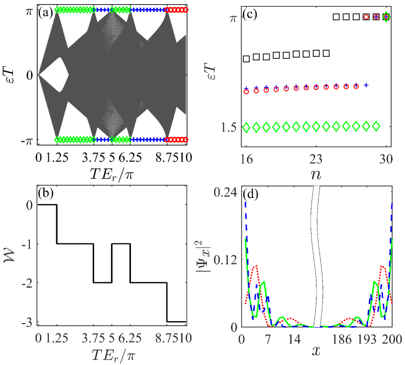
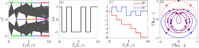
Figures 2(a) and 2(b) show the quasienergy spectrum and the winding number with changing . The parameters are chosen such that the static systems are topologically trivial. The nontrivial phases are induced when the periodic quenching is on [see Fig. 2(a) with being the recoil energy]. For small , Eq. (5) is not fulfilled and a finite band gap exists at the zero quasienergy. With increasing , the gap remains closed due to Case I. However, the gap at is closed and reopened at , , , , and accompanied by the corresponding change of [see Fig. 2(b)]. They correspond to Eq. (11) with , , , , and , respectively. Figure 2(c) shows that the number of degeneracy of the formed bound modes exactly equals to , as required by the bulk-edge correspondence Asbóth et al. (2014). More bound modes are achievable with further increasing . As expected, all the bound modes are highly confined at the edges [see Fig. 2(d)].

To reveal how changes when crosses the phase boundaries, we check the change rate of across the quasienergy at , i.e., at . The Bloch vectors near read with being an infinitesimal. Then we have with . Reminding that is odd, we can easily find that the bands touch at . The change rates of are
| (12) |
with which the change rule of can be obtained.
For , the bands for both and touch at . Equation (12) reveals that crosses along the (or ) direction for (or ) with increasing . This is confirmed by the dashed lines in Figs. 3(a) and 3(b). Since only the first Brillouin zone of the quasienergy is meaningful, abruptly jumps from to keeping the direction unchanged when crosses the phase boundary [see the solid lines in Figs. 3(a) and 3(b)]. Then a closed path with a clockwise wrapping to the origin is formed in Fig. 3(a) with running over . It causes changing from to . Before the phase transition, wraps the origin twice in the clockwise direction [see Fig. 3(b)] indicating . After the phase transition, an anticlockwise path is formed and . Thus decreases (or increases) with increasing across the phase boundary of (or ). This can be confirmed by , where the bands for both and touch at . Figures 3(c) and 3(d) demonstrate the cases that changes from (dashed line) to (solid line) and from (dashed line) to (solid line), respectively.
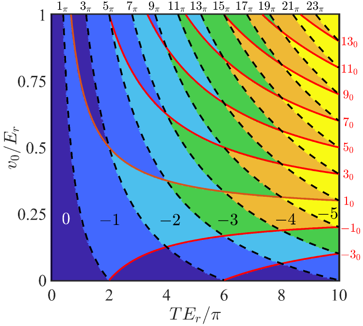
The change of can be verified by the phase diagram in Fig. 4. The solid and dashed lines depict the phase boundaries analytically evaluated from Eq. (11). With increasing , increases through a solid line and decreases through a dashed line. Note that the phases with large and multiple edge modes can be obtained at large . The physics behind this originates from the ability of periodic driving in effectively engineering the long-range hopping Tong et al. (2013). However, we face a tradeoff between the increased number of edge modes and the decreased gap in the quasienergy spectrum. Considering the necessary protection of the edge modes by a nonzero bulk gap, one may not want to push our driving protocol too far. The phase diagram gives a map for experimentally designing the parameters to engineer exotic topological phases. We emphasize that the findings above are qualitatively valid in the general case with (see Appendix A).
IV.2 Periodic quenching in 2D case
Using the protocol Eq. (10), a widely tunable number of edge modes can also be generated in the 2D case. Without loss of generality, we choose . It can be proved that both of Eq. (3) with “” and Eq. (5) do not support phase transition (see Appendix B). Equation (3) with “” reveals the band-touching points with , or , such that Eq. (4) reads
| (13) |
Thus, the bands touch at () for odd (even) .
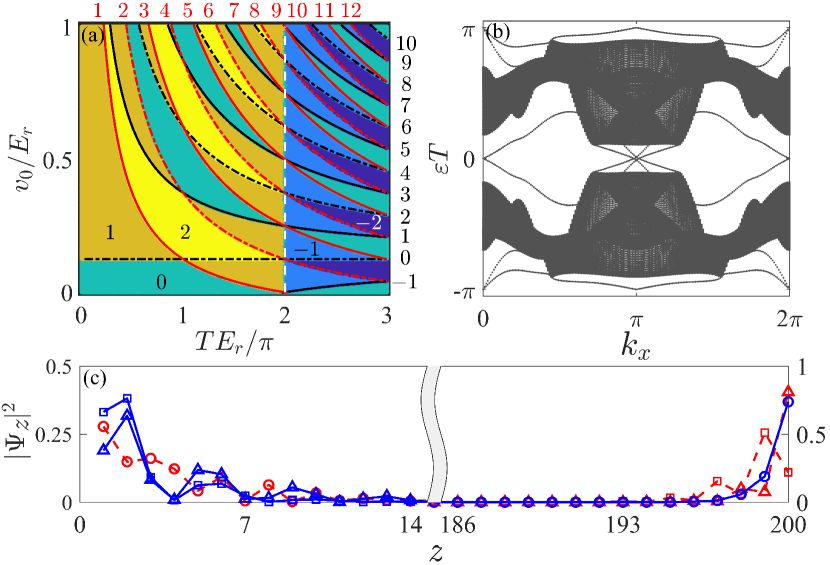
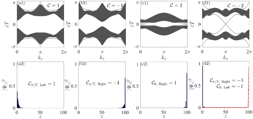
As depicted in the phase diagram Fig. 5(a), a tunable ranging from to can be formed. The boundaries match well with Eq. (13). In the same mechanism, when increases across the phase boundaries, has an abrupt jump in sign at . It causes the change of the wrapping time of to the origin of the BZ. The chirality for and is (see Appendix B). Thus when increases across the phase boundary contributed by these two points, is for odd and for even , respectively. This is verified by the black and red lines in Fig. 5(a). The chirality for and is . Both of the points contribute to being , as verified by the white dashed line in Fig. 5(a).
The quasienergy spectrum in Fig. 5(b) reveals that although , there are six independent edge states. The bulk-edge correspondence can be recovered by considering the respective contribution of - and zero-mode edge states to Rudner et al. (2013); Perez-Piskunow et al. (2014). Figure 5(c) shows the site distribution of the six edge states with a positive group velocity , where the number of the zero and modes are both three. Two of the zero modes locate at the left edge and one at the right, which gives . Two of the modes reside at the right and one at the left, which gives (see Appendix B). The total Chern number is .
V Discussion and Conclusion
Our result is realizable in the state-of-the-art of cold-atom experiments Lin et al. (2011); Huang et al. (2016); Wu et al. (2016); Chen et al. (2018). The topological phase transition in the static case of a 87Rb degenerate gas has been observed in Ref. Wu et al. (2016). The Zeeman splitting , the spin-conserved hopping , and the spin-orbit coupling as high as have been realized. The parameters used in our calculation are under the scope of this experimental achievement. Via pairwisely changing the phase of the running waves between and , no extra burden to the experiment is introduced by our periodic quenching protocol. An estimation for the 87Rb in the optical lattice formed by the red laser gives kHz, which conveys from our phase diagrams in Figs. 4 and 5(a) the scale of the period ms. The topological numbers for our periodic system are hopefully detected by linking numbers Tarnowski et al. (2019) via observing the cyclic evolution governed by of the ground state of , where several periods of driving may be generally needed.
In summary, we have proposed a periodic quenching scheme to generate exotic phases with large topological numbers and multiple edge modes both in 1D and 2D cold-atom systems. Resorting to the periodic switching of the phase of the Raman lattice between and , our scheme can be readily implemented in experiments with existing techniques of synthesizing spin-orbit coupling Lin et al. (2011); Huang et al. (2016); Wu et al. (2016); Chen et al. (2018), and supplies an avenue to controllably design topological devices in an experimentally friendly way.
Acknowledgments
This work is supported by the National Natural Science Foundation (Grant Nos. 11875150, 11834005, 11434011, 11522436, and 11774425), the National Key R&D Program of China (Grant No. 2018YFA0306501), the Beijing Natural Science Foundation (Grant No. Z180013), and the Fundamental Research Funds for the Central Universities of China.
Appendix A Recovered chiral symmetry in the 1D case when
In this appendix, we show that the chiral symmetry in the 1D case when can be recovered by a unitary transformation. This supplies another subtle way to engineer the large topological number in systems belonging to symmetry class D with topological invariant.
The evolution operator is , where (). A unitary transformation converts it to with and . According to Eq. (2), we have with and , where , , and . Then we can obtain with and
| (14) | |||||
Equation (14) reveals that if and have the same symmetry with the same symmetry operator, then would inherit their symmetry. The similar result can be obtained by , which converts into .
Consider that both of in the 1D case possess the chiral symmetry. Choosing , the symmetry in determined by would be broken. Its topological property is characterized by the Majorana number Asbóth et al. (2014); Jiang et al. (2011). We readily find
| (15) |
Following the discussion above, the unitary transformation makes preserve the chiral symmetry of . Thus, its topological property is characterized by the winding number. This gives us another way to realize large topological numbers. It has been proven that the number of - and -mode edge modes relates to the winding number determined by and determined by as Asbóth et al. (2014)
| (16) |
We plot in Figs. 6(a)-6(c) the quasienergy spectrum, the Majorana number determined by , the winding number determined by , and determined by with the change of , respectively. With increasing , the gap is closed and reopened at , , , , and for the quasienergy , and , , , and for the quasienergy . They are clearly reflected by , , and . However, only characterizes the parity of the numbers of the formed edge modes ( for odd pairs and for even pairs), while and obtained by recombining of and according to Eq. (16) equal exactly to the numbers of the zero- and -mode edge modes. Therefore, via the unitary transformations, we have perfectly recovered the bulk-edge correspondence in the system. In Fig. 6(d), we show the trajectory of crossing the quasienergy for the band-touching point . According to Eq. (12), for crosses along the direction. The corresponding changes from to . This verifies again our result for the changing rule of the topological number.
Appendix B Phase transition condition and bulk-edge correspondence in the 2D case
In this appendix, we give the derivation of phase transition condition and the change rule of the topological number in the periodically quenched 2D system.
According to Eqs. (3)-(5), the boundaries of the quasienergy band closing are determined as follows.
Case I: . In the neighbourhood of the band-touching point satisfying this condition, i.e., with being an infinitesimal, we obtain . Then we have
| (17) | |||||
where or . It indicates that at the direction of phase transition, the chirality is zero. Thus, this case has no contribution to the phase transition.
Case II: . Equation (3) determines that the bands touch at satisfying . Substituting this condition into Eq. (4), we obtain . In the neighborhood of , i.e., , we have
| (18) | |||||
| (19) |
which lead to . Thus this case cannot induce a topological phase transition either.
Case III: . Equation (3) requires with or . From Eq. (4), we have
| (20) |
which determines the phase boundaries.
To reveal how changes when crosses the phase boundaries, we examine the changing rate of across the quasienergy or at in both the and directions, i.e., and at . Using , with being an infinitesimal, and Eq. (2), we have
| (21) | |||||
| (22) |
where . Remembering , we conclude that the band touching occurs at the quasienergy for odd and for even . The changing rates of at are
| (23) | |||||
| (24) |
Then . The chirality of band-touching points can be calculated as and . Using Eqs. (21) and (22), we have
| (25) | |||||
| (26) | |||||
where Eq. (11) is used and . According to , we obtain
| (27) | |||||
| (28) | |||||
| (29) |
The bulk-edge correspondence in the 2D case can be revealed from the quasienergy spectra and site distribution of edge modes with positive group velocity (see Fig. 7). Figure 7(a1) has only one pair of -mode edge states. The corresponding is uniquely contributed by one of the pair with positive group velocity, which resides on the left edge [Fig. 7(a2)]. Thus the -mode left-edge state contributes to . Similarly, Figs. 7(b1) and 7(b2) indicate that the -mode right-edge state contributes to , while Figs. 7(c1) and 7(c2) show that the -mode right-edge state contributes to . Figure 7(d1) has one pair of -mode and one pair of -mode edge states. The -mode state resides on the right edge and thus contributes . The -mode state resides on the left edge and gives . Then the total Chern number can be justified.
References
- Thouless et al. (1982) D. J. Thouless, M. Kohmoto, M. P. Nightingale, and M. den Nijs, Phys. Rev. Lett. 49, 405 (1982).
- Hasan and Kane (2010) M. Z. Hasan and C. L. Kane, Rev. Mod. Phys. 82, 3045 (2010).
- Fu et al. (2007) L. Fu, C. L. Kane, and E. J. Mele, Phys. Rev. Lett. 98, 106803 (2007).
- Qi and Zhang (2011) X.-L. Qi and S.-C. Zhang, Rev. Mod. Phys. 83, 1057 (2011).
- Burkov and Balents (2011) A. A. Burkov and L. Balents, Phys. Rev. Lett. 107, 127205 (2011).
- Wan et al. (2011) X. Wan, A. M. Turner, A. Vishwanath, and S. Y. Savrasov, Phys. Rev. B 83, 205101 (2011).
- Lv et al. (2015) B. Q. Lv, H. M. Weng, B. B. Fu, X. P. Wang, H. Miao, J. Ma, P. Richard, X. C. Huang, L. X. Zhao, G. F. Chen, Z. Fang, X. Dai, T. Qian, and H. Ding, Phys. Rev. X 5, 031013 (2015).
- Burkov et al. (2011) A. A. Burkov, M. D. Hook, and L. Balents, Phys. Rev. B 84, 235126 (2011).
- Lu et al. (2015) L. Lu, Z. Wang, D. Ye, L. Ran, L. Fu, J. D. Joannopoulos, and M. Soljačić, Science 349, 622 (2015).
- Xu et al. (2015) S.-Y. Xu, I. Belopolski, N. Alidoust, M. Neupane, G. Bian, C. Zhang, R. Sankar, G. Chang, Z. Yuan, C.-C. Lee, S.-M. Huang, H. Zheng, J. Ma, D. S. Sanchez, B. Wang, A. Bansil, F. Chou, P. P. Shibayev, H. Lin, S. Jia, and M. Z. Hasan, Science 349, 613 (2015).
- Lu et al. (2014) L. Lu, J. D. Joannopoulos, and M. Soljačić, Nature Photonics 8, 821 (2014).
- Khanikaev et al. (2012) A. B. Khanikaev, S. Hossein Mousavi, W.-K. Tse, M. Kargarian, A. H. MacDonald, and G. Shvets, Nature Materials 12, 233 (2012).
- Slobozhanyuk et al. (2016) A. Slobozhanyuk, S. H. Mousavi, X. Ni, D. Smirnova, Y. S. Kivshar, and A. B. Khanikaev, Nature Photonics 11, 130 (2016).
- Maczewsky et al. (2017) L. J. Maczewsky, J. M. Zeuner, S. Nolte, and A. Szameit, Nature Communications 8, 13756 (2017).
- Ozawa et al. (2019) T. Ozawa, H. M. Price, A. Amo, N. Goldman, M. Hafezi, L. Lu, M. C. Rechtsman, D. Schuster, J. Simon, O. Zilberberg, and I. Carusotto, Rev. Mod. Phys. 91, 015006 (2019).
- Wang et al. (2013) J. Wang, B. Lian, H. Zhang, Y. Xu, and S.-C. Zhang, Phys. Rev. Lett. 111, 136801 (2013).
- Fang et al. (2014) C. Fang, M. J. Gilbert, and B. A. Bernevig, Phys. Rev. Lett. 112, 046801 (2014).
- Haldane and Raghu (2008) F. D. M. Haldane and S. Raghu, Phys. Rev. Lett. 100, 013904 (2008).
- Skirlo et al. (2014) S. A. Skirlo, L. Lu, and M. Soljačić, Phys. Rev. Lett. 113, 113904 (2014).
- Skirlo et al. (2015) S. A. Skirlo, L. Lu, Y. Igarashi, Q. Yan, J. Joannopoulos, and M. Soljačić, Phys. Rev. Lett. 115, 253901 (2015).
- Goldman (2009) N. Goldman, Journal of Physics B: Atomic, Molecular and Optical Physics 42, 055302 (2009).
- Yao et al. (2007) W. Yao, A. H. MacDonald, and Q. Niu, Phys. Rev. Lett. 99, 047401 (2007).
- Oka and Aoki (2009) T. Oka and H. Aoki, Phys. Rev. B 79, 081406(R) (2009).
- Lindner et al. (2011) N. H. Lindner, G. Refael, and V. Galitski, Nature Physics 7, 490 (2011).
- Kitagawa et al. (2011) T. Kitagawa, T. Oka, A. Brataas, L. Fu, and E. Demler, Phys. Rev. B 84, 235108 (2011).
- Dóra et al. (2012) B. Dóra, J. Cayssol, F. Simon, and R. Moessner, Phys. Rev. Lett. 108, 056602 (2012).
- Inoue and Tanaka (2010) J.-i. Inoue and A. Tanaka, Phys. Rev. Lett. 105, 017401 (2010).
- Foster et al. (2013) M. S. Foster, M. Dzero, V. Gurarie, and E. A. Yuzbashyan, Phys. Rev. B 88, 104511 (2013).
- Sacramento (2014) P. D. Sacramento, Phys. Rev. E 90, 032138 (2014).
- Bhattacharya et al. (2017) U. Bhattacharya, J. Hutchinson, and A. Dutta, Phys. Rev. B 95, 144304 (2017).
- Fulga and Maksymenko (2016) I. C. Fulga and M. Maksymenko, Phys. Rev. B 93, 075405 (2016).
- Caio et al. (2015) M. D. Caio, N. R. Cooper, and M. J. Bhaseen, Phys. Rev. Lett. 115, 236403 (2015).
- Foster et al. (2014) M. S. Foster, V. Gurarie, M. Dzero, and E. A. Yuzbashyan, Phys. Rev. Lett. 113, 076403 (2014).
- Wang et al. (2017a) L. C. Wang, X. P. Li, and C. F. Li, Phys. Rev. B 95, 104308 (2017a).
- Zhou and Gong (2018) L. Zhou and J. Gong, Phys. Rev. B 97, 245430 (2018).
- Klinovaja et al. (2016) J. Klinovaja, P. Stano, and D. Loss, Phys. Rev. Lett. 116, 176401 (2016).
- Ünal et al. (2019) F. N. Ünal, B. Seradjeh, and A. Eckardt, Phys. Rev. Lett. 122, 253601 (2019).
- Pérez-González et al. (2019) B. Pérez-González, M. Bello, G. Platero, and Á. Gómez-León, arXiv e-prints , arXiv:1903.07678 (2019).
- Mikami et al. (2016) T. Mikami, S. Kitamura, K. Yasuda, N. Tsuji, T. Oka, and H. Aoki, Phys. Rev. B 93, 144307 (2016).
- Xiong et al. (2016) T.-S. Xiong, J. Gong, and J.-H. An, Phys. Rev. B 93, 184306 (2016).
- Lin et al. (2011) Y.-J. Lin, K. Jiménez-García, and I. B. Spielman, Nature 471, 83 (2011).
- Huang et al. (2016) L. Huang, Z. Meng, P. Wang, P. Peng, S.-L. Zhang, L. Chen, D. Li, Q. Zhou, and J. Zhang, Nature Physics 12, 540 (2016).
- Wu et al. (2016) Z. Wu, L. Zhang, W. Sun, X.-T. Xu, B.-Z. Wang, S.-C. Ji, Y. Deng, S. Chen, X.-J. Liu, and J.-W. Pan, Science 354, 83 (2016).
- Chen et al. (2018) H.-R. Chen, K.-Y. Lin, P.-K. Chen, N.-C. Chiu, J.-B. Wang, C.-A. Chen, P.-P. Huang, S.-K. Yip, Y. Kawaguchi, and Y.-J. Lin, Phys. Rev. Lett. 121, 113204 (2018).
- Eckardt (2017) A. Eckardt, Rev. Mod. Phys. 89, 011004 (2017).
- Jünemann et al. (2017) J. Jünemann, A. Piga, S.-J. Ran, M. Lewenstein, M. Rizzi, and A. Bermudez, Phys. Rev. X 7, 031057 (2017).
- Tran et al. (2017) D. T. Tran, A. Dauphin, A. G. Grushin, P. Zoller, and N. Goldman, Science Advances 3, e1701207 (2017).
- Gross and Bloch (2017) C. Gross and I. Bloch, Science 357, 995 (2017).
- Potirniche et al. (2017) I.-D. Potirniche, A. C. Potter, M. Schleier-Smith, A. Vishwanath, and N. Y. Yao, Phys. Rev. Lett. 119, 123601 (2017).
- Wang et al. (2017b) S. Wang, J.-S. Pan, X. Cui, W. Zhang, and W. Yi, Phys. Rev. A 95, 043634 (2017b).
- Price et al. (2017) H. M. Price, T. Ozawa, and N. Goldman, Phys. Rev. A 95, 023607 (2017).
- Zhang et al. (2018) D.-W. Zhang, Y.-Q. Zhu, Y. X. Zhao, H. Yan, and S.-L. Zhu, Advances in Physics 67, 253 (2018).
- Cooper et al. (2019) N. R. Cooper, J. Dalibard, and I. B. Spielman, Rev. Mod. Phys. 91, 015005 (2019).
- Peter et al. (2015) D. Peter, N. Y. Yao, N. Lang, S. D. Huber, M. D. Lukin, and H. P. Büchler, Phys. Rev. A 91, 053617 (2015).
- Sambe (1973) H. Sambe, Phys. Rev. A 7, 2203 (1973).
- Chen et al. (2015) C. Chen, J.-H. An, H.-G. Luo, C. P. Sun, and C. H. Oh, Phys. Rev. A 91, 052122 (2015).
- Jiang et al. (2011) L. Jiang, T. Kitagawa, J. Alicea, A. R. Akhmerov, D. Pekker, G. Refael, J. I. Cirac, E. Demler, M. D. Lukin, and P. Zoller, Phys. Rev. Lett. 106, 220402 (2011).
- Asbóth et al. (2014) J. K. Asbóth, B. Tarasinski, and P. Delplace, Phys. Rev. B 90, 125143 (2014).
- Rodriguez-Vega and Seradjeh (2018) M. Rodriguez-Vega and B. Seradjeh, Phys. Rev. Lett. 121, 036402 (2018).
- Xu et al. (2018) X.-Y. Xu, Q.-Q. Wang, W.-W. Pan, K. Sun, J.-S. Xu, G. Chen, J.-S. Tang, M. Gong, Y.-J. Han, C.-F. Li, and G.-C. Guo, Phys. Rev. Lett. 120, 260501 (2018).
- Tong et al. (2013) Q.-J. Tong, J.-H. An, J. Gong, H.-G. Luo, and C. H. Oh, Phys. Rev. B 87, 201109(R) (2013).
- Liu et al. (2014) X.-J. Liu, K. T. Law, and T. K. Ng, Phys. Rev. Lett. 112, 086401 (2014).
- Liu et al. (2013) X.-J. Liu, Z.-X. Liu, and M. Cheng, Phys. Rev. Lett. 110, 076401 (2013).
- Pan et al. (2015) J.-S. Pan, X.-J. Liu, W. Zhang, W. Yi, and G.-C. Guo, Phys. Rev. Lett. 115, 045303 (2015).
- Chiu et al. (2016) C.-K. Chiu, J. C. Y. Teo, A. P. Schnyder, and S. Ryu, Rev. Mod. Phys. 88, 035005 (2016).
- Kitagawa et al. (2010) T. Kitagawa, E. Berg, M. Rudner, and E. Demler, Phys. Rev. B 82, 235114 (2010).
- Li et al. (2014) L. Li, Z. Xu, and S. Chen, Phys. Rev. B 89, 085111 (2014).
- Sticlet et al. (2012) D. Sticlet, F. Piéchon, J.-N. Fuchs, P. Kalugin, and P. Simon, Phys. Rev. B 85, 165456 (2012).
- Rudner et al. (2013) M. S. Rudner, N. H. Lindner, E. Berg, and M. Levin, Phys. Rev. X 3, 031005 (2013).
- Perez-Piskunow et al. (2014) P. M. Perez-Piskunow, G. Usaj, C. A. Balseiro, and L. E. F. F. Torres, Phys. Rev. B 89, 121401 (2014).
- Tarnowski et al. (2019) M. Tarnowski, F. N. Ünal, N. Fläschner, B. S. Rem, A. Eckardt, K. Sengstock, and C. Weitenberg, Nature Communications 10, 1728 (2019).