Polynomials with symmetric zeros

Abstract

Polynomials whose zeros are symmetric either to the real line or to the unit circle are very important in mathematics and physics. We can classify them into three main classes: the self-conjugate polynomials, whose zeros are symmetric to the real line; the self-inversive polynomials, whose zeros are symmetric to the unit circle; and the self-reciprocal polynomials, whose zeros are symmetric by an inversion with respect to the unit circle followed by a reflection in the real line. Real self-reciprocal polynomials are simultaneously self-conjugate and self-inversive so that their zeros are symmetric to both the real line and the unit circle. In this survey, we present a short review of these polynomials, focusing on the distribution of their zeros.

1 Introduction

In this work, we consider the theory of self-conjugate (SC), self-reciprocal (SR) and self-inversive (SI) polynomials. These are polynomials whose zeros are symmetric either to the real line $\mathbb{R}$ or to the unit circle $\mathbb{S}=\left\{z\in\mathbb{C}:|z|=1\right\}$. The basic properties of these polynomials can be found in the books of Marden [1], Milovanović & al. [2], Sheil-Small [3]. Although these polynomials are very important in both mathematics and physics, it seems that there is no specific review about them; in this work we present a bird’s eye view to this theory, focusing on the zeros of such polynomials. Other aspects of the theory (e.g., irreducibility, norms, analytical properties etc.) are not covered here due to the short space, nonetheless, the interested reader can check many of the references presented in the bibliography to this end.

2 Self-conjugate, Self-reciprocal and Self-inversive polynomials

We begin with some definitions:

Definition 1.

Let $p(z)=p_{0}+p_{1}z+\cdots+p_{n-1}z^{n-1}+p_{n}z^{n}$ be a polynomial of degree $n$ with complex coefficients. We shall introduce three polynomials — namely, the conjugate polynomial $\overline{p}(z)$, the reciprocal polynomial $p^{\ast}(z)$ and the inversive polynomial $p^{\dagger}(z)$ —, that are respectively defined in terms of $p(z)$ as follows:

$$\overline{p}(z) =\overline{p_{0}}+\overline{p_{1}}z+\cdots+\overline{p_{n-1}}z^{n-1}+\overline{p_{n}}z^{n},$$

$$p^{\ast}(z) =p_{n}+p_{n-1}z+\cdots+p_{1}z^{n-1}+p_{0}z^{n},$$

$$p^{\dagger}(z) =\overline{p_{n}}+\overline{p_{n-1}}z+\cdots+\overline{p_{1}}z^{n-1}+\overline{p_{0}}z^{n},$$ (2.1)

where the bar means complex conjugation. Notice that the conjugate, reciprocal and inversive polynomials can also be defined without making reference to the coefficients of $p(z)$:

$$\overline{p}(z)=\overline{p(\overline{z})},\qquad p^{\ast}(z)=z^{n}p\left(1/z\right),\qquad p^{\dagger}(z)=z^{n}\overline{p\left(1/\overline{z}\right)}.$$ (2.2)

From these relations we plainly see that, if $\zeta_{1},\ldots,\zeta_{n}$ are the zeros of a complex polynomial $p(z)$ of degree $n$, then, the zeros of $\overline{p}(z)$ are $\overline{\zeta_{1}},\ldots,\overline{\zeta_{n}}$, the zeros of $p^{\ast}(z)$ are $1/\zeta_{1},\ldots,1/\zeta_{n}$ and, finally, the zeros of $p^{\dagger}(z)$ are $1/\overline{\zeta_{1}},\ldots,1/\overline{\zeta_{n}}$. Thus, if $p(z)$ has $k$ zeros on $\mathbb{R}$, $l$ zeros on the upper half-plane $\mathbb{C}^{+}=\left\{z\in\mathbb{C}:\mathrm{Im}(z)>0\right\}$ and $m$ zeros in the lower half-plane $\mathbb{C}^{-}=\left\{z\in\mathbb{C}:\mathrm{Im}(z)<0\right\}$ so that $k+l+m=n$, then $\overline{p}(z)$ will have the same number $k$ of zeros on $\mathbb{R}$, $l$ zeros in $\mathbb{C}^{-}$ and $m$ zeros in $\mathbb{C}^{+}$. Similarly, if $p(z)$ has $k$ zeros on $\mathbb{S}$, $l$ zeros inside $\mathbb{S}$ and $m$ zeros outside $\mathbb{S}$, so that $k+l+m=n$, then both $p^{\ast}(z)$ as $p^{\dagger}(z)$ will have the same number $k$ of zeros on $\mathbb{S}$, $l$ zeros outside $\mathbb{S}$ and $m$ zeros inside $\mathbb{S}$.

These properties encourage us to introduce the following classes of polynomials:

Definition 2.

A complex polynomial $p(z)$ is called self-conjugate (SC), self-reciprocal (SR) or self-inversive (SI) if, for any zero $\zeta$ of $p(z)$, the complex-conjugate $\overline{\zeta}$, the reciprocal $1/\zeta$ or the reciprocal of the complex-conjugate $1/\overline{\zeta}$ is also a zero of $p(z)$, respectively.

Thus, the zeros of any SC polynomial are all symmetric to the real line $\mathbb{R}$, while the zeros of the any SI polynomial are symmetric to the unit circle $\mathbb{S}$. The zeros of any SR polynomial are obtained by an inversion with respect to the unit circle followed by a reflection in the real line. From this we can establish the following:

Theorem 1.

If $p(z)$ is an SC polynomial of odd degree, then it necessarily has at least one zero on $\mathbb{R}$. Similarly, if $p(z)$ is an SR or SI polynomial of odd degree, then it necessarily has at least one zero on $\mathbb{S}$.

Proof.

From Definition 2 it follows that the number of non-real zeros of an SC polynomial $p(z)$ can only occur in (conjugate) pairs; thus, if $p(z)$ has odd degree, then at least one zero of it must be real. Similarly, the zeros of $p^{\dagger}(z)$ or $p^{\ast}(z)$ that have modulus different from $1$ can only occur in (inversive or reciprocal) pairs as well; thus, if $p(z)$ has odd degree then at least one zero of it must lie on $\mathbb{S}$. ∎

Theorem 2.

The necessary and sufficient condition for a complex polynomial $p(z)$ to be SC, SR or SI is that there exists a complex number $\omega$ of modulus $1$ so that one of the following relations respectively holds:

$$p(z)=\omega\overline{p}(z),\qquad p(z)=\omega p^{\ast}(z),\qquad p(z)=\omega p^{\dagger}(z).$$ (2.3)

Proof.

It is clear in view of (2.1) and (2.2) that these conditions are sufficient. We need to show, therefore, that these conditions are also necessary. Let us suppose first that $p(z)$ is SC. Then, for any zero $\zeta$ of $p(z)$ the complex-conjugate number $\overline{\zeta}$ is also a zero of it. Thus we can write,

$$p(z)=p_{n}\prod_{k=1}^{n}\left(z-\overline{\zeta_{k}}\right)=p_{n}\prod_{k=1}^{n}\overline{\left(\overline{z}-\zeta_{k}\right)}=\left(p_{n}/\overline{p_{n}}\right)\overline{p(\overline{z})}=\omega\bar{p}(z),$$ (2.4)

with $\omega=p_{n}/\overline{p_{n}}$ so that $|\omega|=\left|p_{n}/\overline{p_{n}}\right|=1$. Now, let us suppose that $p(z)$ is SR. Then, for any zero $\zeta$ of $p(z)$ the reciprocal number $1/\zeta$ is also a zero of it; thus,

$$p(z)=p_{n}\prod_{k=1}^{n}\left(z-\frac{1}{\zeta_{k}}\right)=\frac{\left(-1\right)^{n}z^{n}p_{n}}{\zeta_{1}\cdots\zeta_{n}}\prod_{k=1}^{n}\left(\frac{1}{z}-\zeta_{k}\right)=\frac{\left(-1\right)^{n}z^{n}}{\zeta_{1}\cdots\zeta_{n}}p\left(\frac{1}{z}\right)=\omega p^{\ast}(z),$$ (2.5)

with $\omega=\left(-1\right)^{n}/\left(\zeta_{1}\ldots\zeta_{n}\right)=p_{n}/p_{0}$; now, for any zero $\zeta$ of $p(z)$ (which is necessarily different from zero if $p(z)$ is SR), there will be another zero whose value is $1/\zeta$ so that $\left|\zeta_{1}\ldots\zeta_{n}\right|=1$, which implies $|\omega|=1$. The proof for SI polynomials is analogous and will be concealed; it follows that $\omega=p_{n}/\overline{p_{0}}$ in this case. ∎

Now, from (2.1), (2.2) and (2.3) we can conclude that the coefficients of an SC, an SR and an SI polynomial of degree $n$ satisfy, respectively, the following relations:

$$p_{k}=\omega\overline{p_{k}},\qquad p_{k}=\omega p_{n-k},\qquad p_{k}=\omega\overline{p_{n-k}},\qquad|\omega|=1,\qquad 0\leqslant k\leqslant n.$$ (2.6)

We highlight that any real polynomial is SC — in fact, many theorems which are valid for real polynomials are also valid for, or can be easily extended to, SC polynomials.

There also exist polynomials whose zeros are symmetric with respect to both the real line $\mathbb{R}$ and the unit circle $\mathbb{S}$. A polynomial $p(z)$ with this double symmetry is, at the same time, SC and SI (and, hence, SR as well). This is only possible if all the coefficients of $p(z)$ are real, which implies that $\omega=\pm 1$. This suggests the following additional definitions:

Definition 3.

A real self-reciprocal polynomial $p(z)$ that satisfies the relation $p(z)=\omega z^{n}p(1/z)$ will be called a positive self-reciprocal (PSR) polynomial if $\omega=1$ and a negative self-reciprocal (NSR) polynomial if $\omega=-1$.

Thus, the coefficients of any PSR polynomial $p(z)=p_{0}+\cdots+p_{n}z^{n}$ of degree $n$ satisfy the relations $p_{k}=p_{n-k}$ for $0\leqslant k\leqslant n$, while the coefficients of any NSR polynomial $p(z)$ of degree $n$ satisfy the relations $p_{k}=-p_{n-k}$ for $0\leqslant k\leqslant n$; this last condition implies that the middle coefficient of an NSR polynomial of even degree is always zero.

Some elementary properties of PSR and NSR polynomials are the following: first, notice that, if $\zeta$ is a zero of any PSR or NSR polynomial $p(z)$ of degree $n\geqslant 4$, then the three complex numbers $1/\zeta$, $\overline{\zeta}$ and $1/\overline{\zeta}$ are also zeros of $p(z)$. In particular, the number of zeros of such polynomials which are neither on $\mathbb{S}$ or $\mathbb{R}$ is always a multiple of $4$. Besides, any NSR polynomial has $z=1$ as a zero and $p(z)/(z-1)$ is PSR; further, if $p(z)$ has even degree then $z=-1$ is also a zero of it and $p(z)/(z^{2}-1)$ is a PSR polynomial of even degree. In a similar way, any PSR polynomial $p(z)$ of odd degree has $z=-1$ as a zero and $p(z)/(z+1)$ is also PSR. The product of two PSR, or two NSR, polynomials is PSR, while the product of a PSR polynomial with an NSR polynomial is NSR. These statements follow directly from the definitions of such polynomials.

We also mention that any PSR polynomial of even degree (say, $n=2m$) can be written in the following form:

$$p(z)=z^{m}\left[p_{0}\left(z^{m}+\frac{1}{z^{m}}\right)+p_{1}\left(z^{m-1}+\frac{1}{z^{m-1}}\right)+\cdots+p_{m-1}\left(z+\frac{1}{z}\right)\right]+p_{m},$$ (2.7)

an expression that is obtained by using the relations $p_{k}=p_{2m-k}$, $0\leqslant k\leqslant 2m$ and gathering the terms of $p(z)$ with the same coefficients. Furthermore, the expression $Z_{s}(z)=\left(z^{s}+z^{-s}\right)$ for any integer $s$ can be written as a polynomial of degree $s$ in the new variable $x=z+1/z$ (the proof follows easily by induction over $s$); thus, we can write $p(z)=z^{m}q\left(x\right)$, where $q(x)=q_{0}+\cdots+q_{m}x^{m}$ is such that the coefficients $q_{0},\ldots,q_{m}$ are certain functions of $p_{0},\ldots,p_{m}$. From this we can state the following:

Theorem 3.

Let $p(z)$ be a PSR polynomial of even degree $n=2m$. For each pair $\zeta$ and $1/\zeta$ of self-reciprocal zeros of $p(z)$ that lie on $\mathbb{S}$, there is a corresponding zero $\xi$ of the polynomial $q(x)$, as defined above, in the interval $\left[-2,2\right]$ of the real line.

Proof.

For each zero $\zeta$ of $p(x)$ that lie on $S$, write $\zeta=\mathrm{e}^{i\theta}$ for some $\theta\in\mathbb{R}$. Besides, as $q(x)=q(z+1/z)=p(z)/z^{m}$, it follows that $\xi=\zeta+1/\zeta=2\cos\theta$ will be a zero of $q(x)$. This shows us that $\xi$ is limited to the interval $\left[-2,2\right]$ of the real line. Finally, notice that the reciprocal zero $1/\zeta$ of $p(z)$ is mapped to the same zero $\xi$ of $q(x)$. ∎

Finally, remembering that the Chebyshev polynomials of first kind, $T_{n}(z)$, are defined by the formula $T_{n}\left[\tfrac{1}{2}\left(z+z^{-1}\right)\right]=\tfrac{1}{2}\left(z^{n}+z^{-n}\right)$ for $z\in\mathbb{C}$, it follows as well that $q(x)$, and hence any PSR polynomial, can be written as a linear combination of Chebyshev polynomials:

$$q(x)=2\left[p_{0}T_{m}(x)+p_{1}T_{m-1}(x)+\cdots+p_{m-1}T_{1}(x)+\tfrac{1}{2}p_{m}T_{0}(x)\right].$$ (2.8)

3 How these polynomials are related to each other?

In this section, we shall analyze how SC, SR and SI polynomials are related to each other. Let us begin with the relationship between the SR and SI polynomials, which is actually very simple: indeed, from (2.1), (2.2) and (2.3) we can see that each one is nothing but the conjugate polynomial of the other, that is,

$$p^{\dagger}(z)=\overline{p^{\ast}}(z)=\overline{p^{\ast}(\overline{z})},\qquad\text{and}\qquad p^{\ast}(z)=\overline{p^{\dagger}}(z)=\overline{p^{\dagger}(\overline{z})}.$$ (3.1)

Thus, if $p(z)$ is an SR (SI) polynomial, then $\overline{p}(z)$ will be SI (SR) polynomial. Because of this simple relationship, several theorems which are valid for SI polynomials are also valid for SR polynomials and vice versa.

The relationship between SC and SI polynomials is not so easy to perceive. A way of revealing their connection is to make use of a suitable pair of Möbius transformations, that maps the unit circle onto the real line and vice versa, which is often called Cayley transformations , defined through the formulas:

$$M(z)=\left(z-i\right)/\left(z+i\right),\qquad\text{and}\qquad W(z)=-i\left(z+1\right)/\left(z-1\right).$$ (3.2)

This approach was developed in [4], where some algorithms for counting the number of zeros that a complex polynomial has on the unit circle were also formulated.

It is a easy matter to verify that $M(z)$ maps $\mathbb{R}$ onto $\mathbb{S}$ while $W(z)$ maps $\mathbb{S}$ onto $\mathbb{R}$. Besides, $M(z)$ maps the upper (lower) half-plane to the interior (exterior) of $\mathbb{S}$, while $W(z)$ maps the interior (exterior) of $\mathbb{S}$ onto the upper (lower) half-plane. Notice that $W(z)$ can be thought as the inverse of $M(z)$ in the Riemann sphere $\mathbb{C}_{\infty}=\mathbb{C}\cup\{\infty\}$, if we further assume that $M(-i)=\infty$, $M(\infty)=1$, $W(1)=\infty$ and $W(\infty)=-i$.

Given a polynomial $p(z)$ of degree $n$, we define two Möbius-transformed polynomials, namely,

$$Q(z)=(z+i)^{n}p(M(z)),\qquad\text{and}\qquad T(z)=(z-1)^{n}p(W(z)).$$ (3.3)

The following theorem shows us how the zeros of $Q(z)$ and $T(z)$ are related with the zeros of $p(z)$:

Theorem 4.

Let $\zeta_{1},\ldots,\zeta_{n}$ denote the zeros of $p(z)$ and $\eta_{1},\ldots,\eta_{n}$ the respective zeros of $Q(z)$. Provided $p(1)\neq 0$, we have that $\eta_{1}=W(\zeta_{1}),\ldots,\eta_{n}=W(\zeta_{n})$. Similarly, if $\tau_{1},\ldots\tau_{n}$ are the zeros of $T(z)$, then we have $\tau_{1}=M(\zeta_{1}),\ldots,\tau_{n}=M(\zeta_{n})$, provided that $p(-i)\neq 0$.

Proof.

In fact, inverting the expression for $Q(z)$ and evaluating it in any zero $\zeta_{k}$ of $p(z)$ we get that $p(\zeta_{k})=(-i/2)^{n}(\zeta_{k}-1)^{n}Q(W(\zeta_{k}))=0$ for $0\leqslant k\leqslant n$. Provided that $z=1$ is not a zero of $p(z)$ we get that $\eta_{k}=W(\zeta_{k})$ is a zero of $Q(z)$. The proof for the zeros of $T(z)$ is analogous. ∎

This result also shows that $Q(z)$ and $T(z)$ have the same degree as $p(z)$ whenever $p(1)\neq 0$ or $p(-i)\neq 0$, respectively. In fact, if $p(z)$ has a zero at $z=1$ of multiplicity $m$ then $Q(z)$ will be a polynomial of degree $n-m$, the same being true for $T(z)$ if $p(z)$ has a zero of multiplicity $m$ at $z=-i$. This can be explained by the fact that the points $z=1$ and $z=-i$ are mapped to infinity by $W(z)$ and $M(z)$, respectively.

The following theorem shows that the set of SI polynomials are isomorphic to the set of SC polynomials:

Theorem 5.

Let $p(z)$ be an SI polynomial. Then, the transformed polynomial $Q(z)=(z+i)^{n}p(M(z))$ is an SC polynomial. Similarly, if $p(z)$ is an SC polynomial, then $T(z)=(z-1)^{n}p(W(z))$ will be an SI polynomial.

Proof.

Let $\zeta$ and $1/\bar{\zeta}$ be two inversive zeros an SI polynomial $p(z)$. Then, according to Theorem 4, the corresponding zeros of $Q(z)$ will be:

$$W(\zeta)=-i\frac{\zeta+1}{\zeta-1}=\eta\qquad\text{and}\qquad W\left(\frac{1}{\overline{\zeta}}\right)=-i\frac{1/\overline{\zeta}+1}{1/\overline{\zeta}-1}=i\frac{\overline{\zeta}+1}{\overline{\zeta}-1}=\overline{W(\zeta)}=\overline{\eta}.$$ (3.4)

Thus, any pair of zeros of $p(z)$ that are symmetric to the unit circle are mapped in zeros of $Q(z)$ that are symmetric to the real line; because $p(z)$ is SI, it follows that $Q(z)$ is SC. Conversely, let $\zeta$ and $\overline{\zeta}$ be two zeros of an SC polynomial $p(z)$; then the corresponding zeros of $T(z)$ will be:

$$M(\zeta)=\frac{\zeta-i}{\zeta+i}=\tau\qquad\text{and}\qquad M\left(\overline{\zeta}\right)=\frac{\overline{\zeta}-i}{\overline{\zeta}+i}=-\frac{1/\overline{\zeta}+i}{1/\overline{\zeta}-i}=\frac{1}{\overline{M\left(\zeta\right)}}=\frac{1}{\overline{\tau}}.$$ (3.5)

Thus, any pair of zeros of $p(z)$ that are symmetric to the real line are mapped in zeros of $T(z)$ that are symmetric to the unit circle. Because $p(z)$ is SC, it follows that $T(z)$ is SI. ∎

We can also verify that any SI polynomial with $\omega=1$ is mapped to a real polynomial through $M(z)$, as well as, any real polynomial is mapped to an SI polynomial with $\omega=1$ through $W(z)$. Thus, the set of SI polynomials with $\omega=1$ is isomorphic to the set of real polynomials. Besides, an SI polynomial with $\omega\neq 1$ can be transformed into another one with $\omega=1$ by performing a suitable uniform rotation of its zeros. It can also be shown that the action of the Möbius transformation over a PSR polynomial leads to a real polynomial that has only even powers. See [4] for more.

4 Zeros location theorems

In this section, we shall discuss some theorems regarding the distribution of the zeros of SC, SR and SI polynomials on the complex plane. Some general theorems relying on the number of zeros that an arbitrary complex polynomial has inside, on, or outside $\mathbb{S}$ are also discussed. To save space, we shall not present the proofs of these theorems, which can be found in the original works. Other related theorems can be found in Marden’s book [1].

4.1 Polynomials that do not necessarily have symmetric zeros

The following theorems are classics (see [1] for the proofs):

Theorem 6.

(Rouché). Let $q(z)$ and $r(z)$ be polynomials such that $|q(z)|<|r(z)|$ along all points of $\mathbb{S}$. Then, the polynomial $p(z)=q(z)+r(z)$ has the same number of zeros inside $\mathbb{S}$ as the polynomial $r(z)$, counted with multiplicity.

Thus, if a complex polynomial $p(z)=p_{0}+\cdots+p_{k}z^{k}+\cdots+p_{n}z^{n}$ of degree $n$ is such that $\left|p_{k}\right|>\left|p_{0}+\cdots+p_{k-1}+p_{k+1}+\cdots+p_{n}\right|$, then $p(z)$ will have exactly $k$ zeros inside $\mathbb{S}$, counted with multiplicity.

Theorem 7.

(Gauss & Lucas) The zeros of the derivative $p^{\prime}(z)$ of a polynomial $p(z)$ lie all within the convex hull of the zeros of the $p(z)$.

Thereby, if a polynomial $p(z)$ has all its zeros on $\mathbb{S}$, then all the zeros of $p^{\prime}(z)$ will lie in or on $\mathbb{S}$. In particular, the zeros of $p^{\prime}(z)$ will lie on $\mathbb{S}$ if, and only if, they are multiple zeros of $p(z)$.

Theorem 8.

(Cohn) A necessary and sufficient condition for all the zeros of a complex polynomial $p(z)$ to lie on $\mathbb{S}$ is that $p(z)$ is SI and that its derivative $p^{\prime}(z)$ does not have any zero outside $\mathbb{S}$.

Cohn introduced his theorem in [5]. Bonsall & Marden presented a simpler proof of Conh’s theorem in [6] (see also [7]) and applied it to SI polynomials — in fact, this was probably the first paper to use the expression “self-inversive”. Other important result of Cohn is the following: all the zeros of a complex polynomial $p(z)=p_{n}z^{n}+\cdots+p_{0}$ will lie on $\mathbb{S}$ if, and only if, $|p_{n}|=|p_{0}|$ and all the zeros of $p(z)$ do not lie outside $\mathbb{S}$.

Restricting ourselves to polynomials with real coefficients, Eneström & Kakeya [8, 9, 10] independently presented the following theorem:

Theorem 9.

(Eneström & Kakeya) Let $p(z)$ be a polynomial of degree $n$ with real coefficients. If its coefficients are such that $0<p_{0}\leqslant p_{1}\leqslant\cdots\leqslant p_{n-1}\leqslant p_{n}$, then all the zeros of $p(z)$ lie in or on $\mathbb{S}$. Likewise, if the coefficients of $p(z)$ are such that $0<p_{n}\leqslant p_{n-1}\leqslant\cdots\leqslant p_{1}\leqslant p_{0}$, then all the zeros of $p(z)$ lie on or out $\mathbb{S}$.

The following theorems are relatively more recent. The distribution of the zeros of a complex polynomial regarding the unit circle $\mathbb{S}$ was presented by Marden in [1] and slightly enhanced by Jury in [11]:

Theorem 10.

(Marden & Jury) Let $p(z)$ be a complex polynomial of degree $n$ and $p^{\ast}(z)$ its reciprocal. Construct the sequence of polynomials $P_{j}(z)=\sum_{k=0}^{n-j}P_{j,k}z^{k}$ such that $P_{0}(z)=p(z)$ and $P_{j+1}(z)=\overline{p_{j,0}}P_{j}(z)-\overline{p_{j,n-j}}P_{j}^{\ast}(z)$ for $0\leqslant j\leqslant n-1$ so that we have the relations $p_{j+1,k}=\overline{p_{j,0}}p_{j,k}-p_{j,n-j}\overline{p_{j,n-j-k}}$. Let $\delta_{j}$ denote the constant terms of the polynomials $P_{j}(z)$, i.e., $\delta_{j}=p_{j,0}$ and $\varDelta_{k}=\delta_{1}\cdots\delta_{k}$. Thus, if $N$ of the products $\varDelta_{k}$ are negative and $n-N$ of the products $\varDelta_{k}$ are positive so that none of them are zero, then $p(z)$ has $N$ zeros inside $\mathbb{S}$, $n-N$ zeros outside $\mathbb{S}$ and no zero on $\mathbb{S}$. On the other hand, if $\varDelta_{k}\neq 0$ for some $k<n$ but $P_{k+1}(z)=0$, then $p(z)$ has either $n-k$ zeros on $\mathbb{S}$ or $n-k$ zeros symmetric to $\mathbb{S}$. It has additionally $N$ zeros inside $\mathbb{S}$ and $k-N$ zeros outside $\mathbb{S}$.

A simple necessary and sufficient condition for all the zeros of a complex polynomial to lie on $\mathbb{S}$ was presented by Chen in [12]:

Theorem 11.

(Chen) A necessary and sufficient condition for all the zeros of a complex polynomial $p(z)$ of degree $n$ to lie on $\mathbb{S}$ is that there exists a polynomial $q(z)$ of degree $n-m$ whose zeros are all in or on $\mathbb{S}$ and such that $p(z)=z^{m}q(z)+\omega q^{\dagger}(z)$ for some complex number $\omega$ of modulus $1$.

We close this section by mentioning that there exist many other well-known theorems regarding the distribution of the zeros of complex polynomials. We can cite, for example, the famous rule of Descartes (the number of positive zeros of a real polynomial is limited from above by the number of sign variations in the ordered sequence of its coefficients), the Sturm Theorem (the exact number of zeros that a real polynomial has in a given interval $(a,b]$ of the real line is determined by the formula $N=\mathrm{var}\left[S(b)\right]-\mathrm{var}\left[S(a)\right]$, where $\mathrm{var}\left[S(\xi)\right]$ means the number of sign variations of the Sturm sequence $S(x)$ evaluated at $x=\xi$) and Kronecker Theorem (if all the zeros of a monic polynomial with integer coefficients lie on the unit circle, then all these zeros are indeed roots of unity), see [1] for more. There are still other important theorems relying on matrix methods and quadratic forms that were developed by several authors as Cohn, Schur, Hermite, Sylvester, Hurwitz, Krein, among others, see [13].

4.2 Real self-reciprocal polynomials

Let us now consider real SR polynomials. The theorems below are usually applied to PSR polynomials, but some of them can be extended to NSR polynomials as well.

An analogue of Eneström-Kakeya theorem for PSR polynomials was found by Chen in [12] and then, in a slightly stronger version, by Chinen in [14]:

Theorem 12.

(Chen & Chinen) Let $p(z)$ be a PSR polynomial of degree $n$ that is written in the form $p(z)=p_{0}+p_{1}z+\cdots+p_{k}z^{k}+p_{k}z^{n-k}+p_{k-1}z^{n-k+1}+\cdots+p_{0}z^{n}$ and such that $0<p_{k}<p_{k-1}<\cdots<p_{1}<p_{0}$. Then all the zeros of $p(z)$ are on $\mathbb{S}$.

Going in the same direction, Choo found in [15] the following condition:

Theorem 13.

(Choo) Let $p(z)$ be a PSR polynomial of degree $n$ and such that its coefficients satisfy the following conditions: $np_{n}\geqslant\left(n-1\right)p_{n-1}\geqslant\cdots\geqslant\left(k+1\right)p_{k+1}>0$ and $\left(k+1\right)p_{k+1}\geqslant\sum_{j=0}^{k}\left|\left(j+1\right)p_{j+1}-jp_{j}\right|$ for $0\leqslant k\leqslant n-1$ Then, all the zeros of $p(z)$ are on $\mathbb{S}$.

Lakatos discussed the separation of the zeros on the unit circle of PSR polynomials in [16]; she also found several sufficient conditions for their zeros to be all on $\mathbb{S}$. One of the main theorems is the following:

Theorem 14.

(Lakatos) Let $p(z)$ be a PSR polynomial of degree $n>2$. If $\left|p_{n}\right|\geqslant\sum_{k=1}^{n-1}\left|p_{n}-p_{k}\right|$, then all the zeros of $p(z)$ lie on $\mathbb{S}$. Moreover, the zeros of $p(z)$ are all simple, except when the equality takes place.

For PSR polynomials of odd degree, Lakatos & Losonczi [17] found a stronger version of this result:

Theorem 15.

(Lakatos & Losonczi) Let $p(z)$ be a PSR polynomial of odd degree, say $n=2m+1$. If $\left|p_{2m+1}\right|\geqslant\cos^{2}(\phi_{m})\sum_{k=1}^{2m}\left|p_{2m+1}-p_{k}\right|$, where $\phi_{m}=\pi/\left[4\left(m+1\right)\right]$, then all the zeros of $p(z)$ lie on $\mathbb{S}$. The zeros are simple except when the equality is strict.

Theorem 14 was generalized further by Lakatos & Losonczi in [18]:

Theorem 16.

(Lakatos & Losonczi) All zeros of a PSR polynomial $p(z)$ of degree $n>2$ lie on $\mathbb{S}$ if the following conditions hold: $\left|p_{n}+r\right|\geqslant\sum_{k=1}^{n-1}\left|p_{k}-p_{n}+r\right|$, $p_{n}r\geqslant 0$ and $\left|p_{n}\right|\geqslant\left|r\right|$, for $r\in\mathbb{R}$.

Other conditions for all the zeros of a PSR polynomial to lie on $\mathbb{S}$ was presented by Kwon in [19]. In its simplest form, Kown’s theorem can be enunciated as follows:

Theorem 17.

(Kwon) Let $p(z)$ be a PSR polynomial of even degree $n\geqslant 2$ whose leading coefficient $p_{n}$ is positive and $p_{0}\leqslant p_{1}\leqslant\cdots\leqslant p_{n}$. In this case, all the zeros of $p(z)$ will lie on $\mathbb{S}$ if, either $p_{n/2}\geqslant\sum_{k=0}^{n}\left|p_{k}-p_{n/2}\right|$, or $p(1)\geqslant 0$ and $p_{n}\geqslant\frac{1}{2}\sum_{k=1}^{n-1}\left|p_{k}-p_{n/2}\right|$.

Modified forms of this theorem hold for the PSR polynomials of odd degree and for the case where the coefficients of $p(z)$ do not have the ordination above — see [19] for these cases. Kwon also found conditions for all but two zeros of $p(z)$ to lie on $\mathbb{S}$ in [20], which is relevant to the theory of Salem polynomials — see Section 5.

Other interesting results are the following: Konvalina & Matache [21] found conditions under which a PSR polynomial has at least one non-real zero on $\mathbb{S}$. Kim & Park [22] and then Kim and Lee [23] presented conditions for which all the zeros of certain PSR polynomials lie on $\mathbb{S}$ (some open cases were also addressed by Botta & al. in [24]). Suzuki [25] presented necessary and sufficient conditions, relying on matrix algebra and differential equations, for all the zeros of PSR polynomials to lie on $\mathbb{S}$. In [26] Botta & al. studied the distribution of the zeros of PSR polynomials with a small perturbation in their coefficients. Real SR polynomials of height $1$ — namely, special cases of Littlewood, Newman and Borwein polynomials — were studied by several authors, see [27, 28, 29, 30, 31, 32, 33, 34, 35] and references therein. Zeros of the so-called Ramanujan Polynomials and generalizations were analyzed in [37, 38, 39]. Finally, the Galois theory of PSR polynomials was studied in [40] by Lindstrøm, who showed that any PSR polynomial of degree less than $10$ can be solved by radicals.

4.3 Complex self-reciprocal and self-inversive polynomials

Let us consider now the case of complex SR polynomials and SI polynomials. Here we remark that many of the theorems that hold for SI polynomials either also hold for SR polynomials or can be easily adapted to this case (the opposite is also true).

Theorem 18.

(Cohn) An SI polynomial $p(z)$ has as many zeros outside $\mathbb{S}$ as does its derivative $p^{\prime}(z)$.

This follows directly from Cohn’s Theorem 8 for the case where $p(z)$ is SI. Besides, we can also conclude from this that the derivative of $p(z)$ has no zeros on $\mathbb{S}$ except at the multiple zeros of $p(z)$. Furthermore, if an SI polynomial $p(z)$ of degree $n$ has exactly $k$ zeros on $\mathbb{S}$, while its derivative has exactly $l$ zeros in or on $\mathbb{S}$, both counted with multiplicity, then $n=2(l+1)-k$.

O’Hara & Rodriguez [41] showed that the following conditions are always satisfied by SI polynomials whose zeros are all on $\mathbb{S}$:

Theorem 19.

(O’Hara & Rodriguez) Let $p(z)$ be an SI polynomial of degree $n$ whose zeros are all on $\mathbb{S}$. Then, the following inequality holds: $\sum_{j=0}^{n}|p_{j}|^{2}\leqslant\left\|p(z)\right\|^{2}$, where $\left\|p(z)\right\|$ denotes the maximum modulus of $p(z)$ on the unit circle; besides, if this inequality is strict then the zeros of $p(z)$ are rotations of $n$th roots of unity. Moreover, the following inequalities are also satisfied: $\left|a_{k}\right|\leqslant\tfrac{1}{2}\left\|p(z)\right\|$ if $k\neq n/2$ and $\left|a_{k}\right|\leqslant\tfrac{\sqrt{2}}{2}\left\|p(z)\right\|$ for $k=n/2$.

Schinzel in [42], generalized Lakatos Theorem 14 for SI polynomials:

Theorem 20.

(Schinzel) Let $p(z)$ be an SI polynomial of degree $n$. If the inequality $\left|p_{n}\right|\geqslant\inf_{a,b\in\mathbb{C}:|b|=1}\sum_{k=0}^{n}\left|ap_{k}-b^{n-k}p_{n}\right|$, then all the zeros of $p(z)$ lie on $\mathbb{S}$. These zero are simple whenever the equality is strict.

In a similar way, Losonczi & Schinzel [43] generalized theorem 15 for the SI case:

Theorem 21.

(Losonczi & Schinzel) Let $p(z)$ be an SI polynomial of odd degree, i.e. $n=2m+1$. If $\left|p_{2m+1}\right|\geqslant\cos^{2}\left(\phi_{m}\right)\inf_{a,b\in\mathbb{C}:|b|=1}\sum_{k=1}^{2m+1}\left|ap_{k}-b^{2m+1-k}p_{2m+1}\right|$, where $\phi_{m}=\pi/\left[4\left(m+1\right)\right]$, then all the zeros of $p(z)$ lie on $\mathbb{S}$. The zeros are simple except when the equality is strict.

Another sufficient condition for all the zeros of an SI polynomial to lie on $\mathbb{S}$ was presented by Lakatos & Losonczi in [44]:

Theorem 22.

(Lakatos & Losonczi) Let $p(z)$ be an SI polynomial of degree $n$ and suppose that the inequality $\left|p_{n}\right|\geqslant\frac{1}{2}\sum_{k=1}^{n-1}\left|p_{k}\right|$ holds. Then, all the zeros of $p(z)$ lie on $\mathbb{S}$. Moreover, the zeros are all simple except when an equality takes place.

In [45] Lakatos & Losonczi also formulated a theorem that contains as special cases many of the previous results:

Theorem 23.

(Lakatos & Losonczi) Let $p(z)=p_{0}+\cdots+p_{n}z^{n}$ be an SI polynomial of degree $n\geqslant 2$ and $a$, $b$ and $c$ be complex numbers such that $a\neq 0$, $|b|=1$ and $c/p_{n}\in\mathbb{R}$, $0\leqslant c/p_{n}\leqslant 1$. If $\left|p_{n}+c\right|\geqslant\left|ap_{0}-b^{n}p_{n}\right|+\sum_{k=1}^{n-1}\left|ap_{k}-b^{n-k}\left(c-p_{n}\right)\right|+\left|ap_{n}-p_{n}\right|$, then, all the zeros of $p(z)$ lie on $\mathbb{S}$. Moreover, these zeros are simple if the inequality is strict.

In [46] Losonczi presented the following necessary and sufficient conditions for all the zeros of a (complex) SR polynomial of even degree to lie on $\mathbb{S}$:

Theorem 24.

(Losonczi) Let $p(z)$ be a monic complex SR polynomial of even degree, say $n=2m$. Then, all the zeros of $p(z)$ will lie on $\mathbb{S}$ if, and only if, there exist real numbers $\alpha_{1},\ldots,\alpha_{2m}$, all with moduli less than or equal to $2$, that satisfy the inequalities: $p_{k}=\left(-1\right)^{k}\sum_{l=0}^{\left[k/2\right]}\binom{m-k+2l}{l}\sigma_{k-2l}^{2m}\left(\alpha_{1},\ldots,\alpha_{2m}\right)$, $0\leqslant k\leqslant m$, where $\sigma_{k}^{2m}\left(\alpha_{1},\ldots,\alpha_{2m}\right)$ denotes the $k$th elementary symmetric function in the $2m$ variables $\alpha_{1},\ldots,\alpha_{2m}$.

Losonczi in [46] also showed that if all the zeros of a complex monic reciprocal polynomial are on $\mathbb{S}$ then its coefficients are all real and satisfy the inequality $\left|p_{n}\right|\leqslant\binom{n}{k}$ for $0\leqslant k\leqslant n$.

The theorems above give conditions for all the zeros of SI or SR polynomials to lie on $\mathbb{S}$. In many cases, however, we need to verify if a polynomial has a given number of zeros (or none) on the unit circle. Considering this problem, Vieira in [47] found sufficient conditions for an SI polynomial of degree $n$ to have a determined number of zeros on the unit circle. In terms of the length $L\left[p(z)\right]=\left|p_{0}\right|+\cdots+\left|p_{n}\right|$ of a polynomial $p(z)$ of degree $n$, this theorem can be stated as follows:

Theorem 25.

(Vieira) Let $p(z)$ be an SI polynomial of degree $n$. If the inequality $\left|p_{n-m}\right|\geqslant\tfrac{1}{4}\left(\tfrac{n}{n-m}\right)L\left[p(z)\right]$, $m<n/2$, holds true, then $p(z)$ will have exactly $n-2m$ zeros on $\mathbb{S}$; besides, all these zeros are simple when the inequality is strict. Moreover, $p(z)$ will have no zero on $\mathbb{S}$ if, for $n$ even and $m=n/2$, the inequality $\left|p_{m}\right|>\frac{1}{2}L\left[p(z)\right]$ is satisfied.

The case $m=0$ corresponds to Lakatos & Losonczi Theorem 14 for all the zeros of $p(z)$ to lie on $\mathbb{S}$. The necessary counterpart of this theorem was considered by Stankov in [48], with an application to the theory of Salem numbers — see Section 5.1.

Other results on the distribution of zeros of SI polynomials include the following: Sinclair & Vaaler [49] showed that a monic SI polynomial $p(z)$ of degree $n$ satisfying the inequalities $L^{r}\left[p(z)\right]\leqslant 2+2^{r}\left(n-1\right)^{1-r}$ or $L^{r}\left[p(z)\right]\leqslant 2+2^{r}\left(l-2\right)^{1-r}$, where $r\geqslant 1$, $L^{r}\left[p(z)\right]=\left|p_{0}\right|^{r}+\cdots+\left|p_{n}\right|^{r}$ and $l$ is the number of non-null terms of $p(z)$, has all their zeros on $\mathbb{S}$; the authors also studied the geometry of SI polynomials whose zeros are all on $\mathbb{S}$. Choo & Kim applied Theorem 11 to SI polynomials in [50]. Hypergeometric polynomials with all their zeros on $\mathbb{S}$ were considered in [51, 52]. Kim [53] also obtained SI polynomials which are related to Jacobi polynomials. Ito & Wimmer [54] studied SI polynomial operators in Hilbert space whose spectrum is on $\mathbb{S}$.

5 Where these polynomials are found?

In this section, we shall briefly discuss some important or recent applications of the theory of polynomials with symmetric zeros. We remark, however, that our selection is by no means exhaustive: for example, SR and SI polynomials also find applications in many fields of mathematics (e.g., information and coding theory [55], algebraic curves over a finite field and cryptography [56], elliptic functions [57], number theory [58] etc.) and physics (e.g., Lee-Yang theorem in statistical physics [59], Poincaré Polynomials defined on Calabi-Yau manifolds of superstring theory [60] etc.).

5.1 Polynomials with small Mahler measure

Given a monic polynomial $p(z)$ of degree $n$, with integer coefficients, the Mahler measure of $p(z)$, denoted by $M[p(z)]$, is defined as the product of the modulus of all those zeros of $p(z)$ that lie in the exterior of $\mathbb{S}$ [61]. That is,

$$M[p(z)]=\prod_{i=1}^{n}\max\left\{1,\left|\zeta_{i}\right|\right\},$$ (5.1)

where $\zeta_{1},\ldots,\zeta_{n}$ are the zeros of $p(z)$. Thus, if a monic integer polynomial $p(z)$ has all its zeros in or on the unit circle, we have $M[p(z)]=1$; in particular, all cyclotomic polynomials (which are PSR polynomials whose zeros are the primitive roots of unity, see [1]) have Mahler measure equal to $1$. In a sense, the Mahler measure of a polynomial $p(z)$ measures how close it is to the cyclotomic polynomials. Therefore, it is natural to raise the following:

Problem 1.

(Mahler) Find the monic, integer, non-cyclotomic polynomial with the smallest Mahler measure.

This is an 80 years old open problem of mathematics. Of course, we can expect that the polynomials with the smallest Mahler measure be among those with only a few number of zeros outside $\mathbb{S}$, in particular among those with only one zero outside of $\mathbb{S}$. A monic integer polynomial that has exactly one zero outside $\mathbb{S}$ is called a Pisot polynomial and its unique zero of modulus greater than $1$ is called its Pisot number [62]. A breakthrough towards the solution of Mahler’s problem was given by Smyth in [63]:

Theorem 26.

(Smyth) The Pisot polynomial $S(z)=z^{3}-z-1$ is the polynomial with smallest Mahler measure among the set of all monic, integer and non-SR polynomials. Its Mahler measure is given by the value of its Pisot number, which is,

$$\sigma=\sqrt[3]{\tfrac{1}{2}+\tfrac{1}{2}\sqrt{\tfrac{23}{27}}}+\sqrt[3]{\tfrac{1}{2}-\tfrac{1}{2}\sqrt{\tfrac{23}{27}}}\approx 1.32471795724.$$ (5.2)

The Mahler problem is, however, still open for SR polynomials. A monic integer SR polynomial with exactly two (real and positive) zeros (say, $\zeta$ and $1/\zeta$) not lying on $\mathbb{S}$ is called a Salem polynomial [62, 64]. It can be shown that a Pisot polynomial with at least one zero on $\mathbb{S}$ is also a Salem polynomial. The unique positive zero greater than one of a Salem polynomial is called its Salem number, which also equals the value of its Mahler measure. A Salem number $s$ is said to be small if $s<\sigma$; up to date, only $47$ small Salem numbers are known [65, 66] and the smallest known one was found about 80 years ago by Lehmer [67]. This gave place to the following:

Conjecture 1.

(Lehmer) The monic integer polynomial with the smallest Mahler measure is the Lehmer polynomial $\mathcal{L}(z)=z^{10}+z^{9}-z^{7}-z^{6}-z^{5}-z^{4}-z^{3}+z+1$, a Salem polynomial whose Mahler measure is $\varLambda\approx 1.17628081826$, known as Lehmer’s constant.

The proof of this conjecture is also an open problem. To be fair, we do not even know if there exists a smallest Salem number at all. This is the content of another problem raised by Lehmer:

Problem 2.

(Lehmer) Answer whether there exists or not a positive number $\epsilon$ such that the Mahler measure of any monic, integer and non-cyclotomic polynomial $p(z)$ satisfies the inequality $M[p(z)]>1+\epsilon$.

Lehmer’s polynomial also appears in connection with several fields of mathematics. Many examples are discussed in Hironaka’s paper [68]; here we shall only present an amazing identity found by Bailey & Broadhurst in [69] in their works on polylogarithm ladders: if $\lambda$ is any zero of the aforementioned Lehmer’s polynomial $\mathcal{L}(z)$, then,

$$\frac{\left(\lambda^{315}-1\right)\left(\lambda^{210}-1\right)\left(\lambda^{126}-1\right)^{2}\left(\lambda^{90}-1\right)\left(\lambda^{3}-1\right)^{3}\left(\lambda^{2}-1\right)^{5}\left(\lambda-1\right)^{3}}{\left(\lambda^{630}-1\right)\left(\lambda^{35}-1\right)\left(\lambda^{15}-1\right)^{2}\left(\lambda^{14}-1\right)^{2}\left(\lambda^{5}-1\right)^{6}\lambda^{68}}=1.$$ (5.3)

5.2 Knot theory

A knot is a closed, non-intersecting, one-dimensional curve embedded on $\mathbb{R}^{3}$ [70]. Knot theory studies topological properties of knots as, for example, criteria under which a knot can be unknot, conditions for the equivalency between knots, the classification of prime knots etc. — see [70] for the corresponding definitions. In Figure 5.1 we plotted all prime knots up to six crossings.

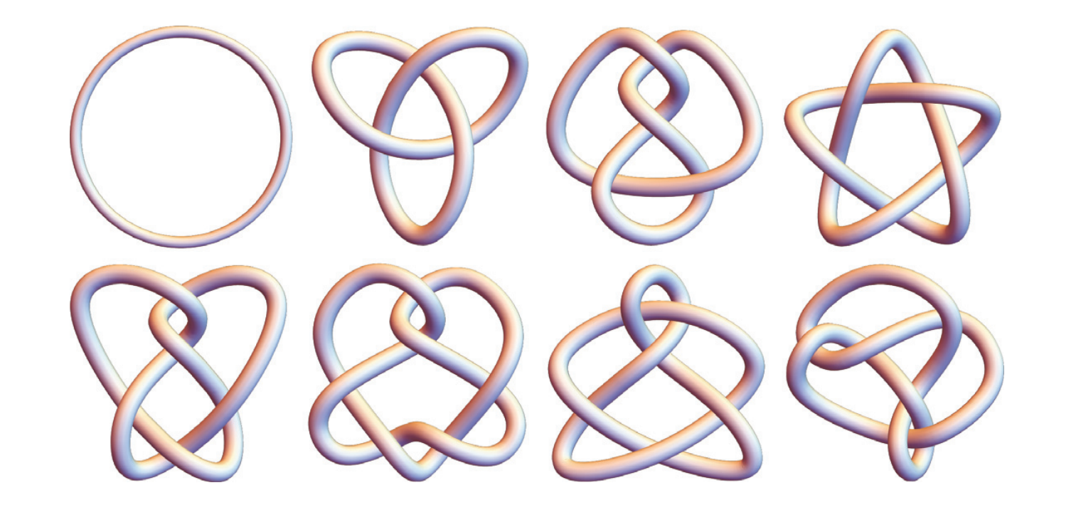
Figure 5.1: A table of prime knots up to six crossings. In the Alexander-Briggs notation these knots are, in order, $0_{1}$, $3_{1}$, $4_{1}$, $5_{1}$, $5_{2}$, $6_{1}$, $6_{2}$ and $6_{3}$.

One of the most important questions in knot theory is to determine whether or not two knots are equivalent. This, however, is not an easy task. A way of attacking this question is to look for abstract objects — mainly the so-called knot invariants — rather than to the knots themselves. A knot invariant is a (topologic, combinatorial, algebraic etc.) quantity that can be computed for any knot and that is always the same for equivalents knots. An important class of knot invariants is constituted by the so-called Knot Polynomials. Knot polynomials were introduced in 1928 by Alexander [71]. They consist in polynomials with integer coefficients that can be written down for every knot. For about 60 years since its creation, Alexander polynomials were the only known kind of knot polynomial. It was only in 1985 that Jones [72] came up with a new kind of knot polynomials — today known as Jones polynomials — and since then other kinds were discovered as well, see [70].

Knot	Alexander polynomial $\varDelta(t)$	Knot	Alexander polynomial $\varDelta(t)$
$0_{1}$	$1$	$5_{2}$	$2-3t+2t^{2}$
$3_{1}$	$1-t+t^{2}$	$6_{1}$	$2-5t+2t^{2}$
$4_{1}$	$1-3t+t^{2}$	$6_{2}$	$1-3t+3t^{2}-3t^{3}+t^{4}$
$5_{1}$	$1-t+t^{2}-t^{3}+t^{4}$	$6_{3}$	$1-3t+5t^{2}-3t^{3}+t^{4}$

Table 1: Alexander polynomials for prime knots up to six crossings.

What is interesting for us here is that the Alexander polynomials are PSR polynomials of even degree (say, $n=2m$) and with integer coefficients. Thus, they have the following general form:

$$\varDelta(t)=\delta_{0}+\delta_{1}+\cdots+\delta_{m-1}t^{m-1}+\delta_{m}t^{m}+\delta_{m-1}t^{m+1}+\cdots+\delta_{1}t^{2m-1}+\delta_{0}t^{2m},$$ (5.4)

where $\delta_{i}\in\mathbb{N}$, $0\leqslant i\leqslant m$. In table 1 we present the Alexander polynomials for the prime knots up to six crossings.

Knots theory finds applications in many fields of mathematics in physics — see [70]. In mathematics, we can cite a very interesting connection between Alexander polynomials and the theory of Salem numbers: more precisely, the Alexander polynomial associated with the so-called Pretzel Knot $\mathcal{P}(-2,3,7)$ is nothing but the Lehmer polynomial $\mathcal{L}(z)$ introduced in Section 5.1; it is indeed the Alexander polynomial with the smallest Mahler measure [73]. In physics, knot theory is connected with quantum groups and it also can be used to one construct solutions of the Yang-Baxter equation [74] through a method called baxterization of braid groups.

5.3 Bethe Equations

The Bethe Equations were introduced in 1931 by Hans Bethe [75] together with his powerful method — the so-called Bethe Ansatz method — for solving spectral problems associated with exactly integrable models of statistical mechanics. They consist in a system of coupled and non-linear equations that ensure the consistency of the Bethe Ansatz. In fact, for the XXZ Heisenberg spin chain, the Bethe Equations consist in a coupled system of trigonometric equations; however, after a change of variables is performed, we can write them in the following rational form:

$$x_{i}^{L}=\left(-1\right)^{N-1}\prod_{k=1,k\neq i}^{N}\frac{x_{i}x_{k}-2\varDelta x_{i}+1}{x_{i}x_{k}-2\varDelta x_{k}+1},\qquad 1\leqslant i\leqslant N,$$ (5.5)

where $L\in\mathbb{N}$ is the length of the chain, $N\in\mathbb{N}$ is the excitation number and $\varDelta\in\mathbb{R}$ is the so-called anisotropy parameter. A solution of (5.5) consists in a (non-ordered) set $X=\left\{x_{1},\ldots,x_{N}\right\}$ of the unknowns $x_{1},\ldots,x_{N}$ so that (5.5) is satisfied. Notice that the Bethe equations satisfy the important relation $x_{1}^{L}x_{2}^{L}\cdots x_{N}^{L}=1$, which suggests an inversive symmetry of their zeros.

In [76], Vieira and Lima-Santos showed that the solutions of (5.5), for $N=2$ and arbitrary $L$, are given in terms of the zeros of certain SI polynomials. In fact, (5.5) becomes a system of two coupled algebraic equations for $N=2$, namely,

$$x_{1}^{L}=-\frac{x_{1}x_{2}-2\varDelta x_{1}+1}{x_{1}x_{2}-2\varDelta x_{2}+1},\qquad\text{and}\qquad x_{2}^{L}=-\frac{x_{1}x_{2}-2\varDelta x_{2}+1}{x_{1}x_{2}-2\varDelta x_{1}+1}.$$ (5.6)

Now, from the relation $x_{1}^{L}x_{2}^{L}=1$ we can eliminate one of the unknowns in (5.6) — for instance, by setting $x_{2}=\omega_{a}/x_{1}$, where $\omega_{a}=\exp\left(2\pi ia/L\right)$, $1\leqslant a\leqslant L$, are the roots of unity of degree $L$. Replacing these values for $x_{2}$ into (5.6), we obtain the following polynomial equations fixing $x_{1}$:

$$p_{a}(z)=\left(1+\omega_{a}\right)z^{L}-2\varDelta\omega_{a}z^{L-1}-2\varDelta z+\left(1+\omega_{a}\right)=0,\qquad 1\leqslant a\leqslant L,$$ (5.7)

We can easily verify that the polynomial $p_{a}(z)$ are SI for each value of $a$. They also satisfy the relations $p_{a}(z)=z^{L}p(\omega_{a}/z)$, $1\leqslant a\leqslant L$, which means that the solutions of (5.6) have the general form $X=\left\{\zeta,\omega_{a}/\zeta\right\}$ for $\zeta$ any zero of $p_{a}(z)$. In [76] the distribution of the zeros of the polynomials $p_{a}(z)$ was analyzed through an application of Vieira’s Theorem 25. It was shown that the exact behaviour of the zeros of the polynomials $p_{a}(z)$, for each $a$, depends on two critical values of $\varDelta$, namely,

$$\varDelta_{a}^{(1)}=\tfrac{1}{2}\left|\omega_{a}+1\right|,\qquad\text{and}\qquad\varDelta_{a}^{(2)}=\tfrac{1}{2}\left(\tfrac{L}{L-2}\right)\left|\omega_{a}+1\right|,$$ (5.8)

as follows: if $|\varDelta|\leqslant\varDelta_{a}^{(1)}$, then all the zeros of $p_{a}(z)$ are on $\mathbb{S}$; if $|\varDelta|\geqslant\varDelta_{a}^{(2)}$, then all the zeros of $p_{a}(z)$ but two are on $\mathbb{S}$; (see [76] for the case $\varDelta_{a}^{(1)}<|\varDelta|<\varDelta_{a}^{(2)}$ and more details).

Finally, we highlight that the polynomial $p_{a}(z)$ becomes a Salem polynomial for $a=L$ and integer values of $\varDelta$. This was one of the first appearances of Salem polynomials in physics.

5.4 Orthogonal polynomials

An infinite sequence $\mathcal{P}=\left\{P_{n}(z)\right\}_{n\in\mathbb{N}}$ of polynomials $P_{n}(z)$ of degree $n$ is said to be an orthogonal polynomial sequence on the interval $(l,r)$ of the real line if there exists a function $w(x)$, positive in $(l,r)\in\mathbb{R}$, such that,

$$\int_{l}^{r}P_{m}(z)P_{n}(z)w(z)dz=\begin{cases}K_{n},&m=n,\\ 0,&m\neq n,\end{cases}\qquad m,n\in\mathbb{N},$$ (5.9)

where $K_{0}$, $K_{1}$ etc. are positive numbers. Orthogonal polynomial sequences on the real line have many interesting and important properties — see [77].

Hermite polynomials	Möbius-transformed Hermite polynomials
$H_{0}(z)=1$	$\mathcal{H}_{0}(z)=1$
$H_{1}(z)=2z$	$\mathcal{H}_{1}(z)=-2i-2iz$
$H_{2}(z)=-2+4z^{2}$	$\mathcal{H}_{2}(z)=-6-4z-6z^{2}$
$H_{3}(z)=-12z+8z^{3}$	$\mathcal{H}_{3}(z)=20i+12iz+12iz^{2}+20iz^{3}$
$H_{4}(z)=12-48z^{2}+16z^{4}$	$\mathcal{H}_{4}(z)=76+16z+72z^{2}+16z^{3}+76z^{4}$

Table 2: Hermite and Möbius-transformed Hermite polynomials, up to $4$th degree.

Very recently, Vieira & Botta [78, 79] studied the action of Möbius transformations over orthogonal polynomial sequences on the real line. In particular, they showed that the infinite sequence $\mathcal{T}=\left\{T_{n}(z)\right\}_{n\in\mathbb{N}}$ of the Möbius-transformed polynomials $T_{n}(z)=(z-1)^{n}P_{n}\left(W(z)\right)$, where $W(z)=-i(z+1)/(z-1)$, is an SR and/or SI polynomial sequence with all their zeros on the unit circle $\mathbb{S}$ — see Table 2 for an example. We highlight that the polynomials $T_{n}(z)\in\mathcal{T}$ also have properties similar to the original polynomials $P_{n}(z)\in\mathcal{P}$ as, for instance, they satisfy a type of orthogonality condition on the unit circle and a three-term recurrence relation, their zeros lie all on $\mathbb{S}$ and are simple, for $n\geqslant 1$ the zeros of $T_{n}(z)$ interlaces with those of $T_{n+1}(z)$ and so on — see [78, 79] for more details.

6 Conclusions

In this work, we reviewed the theory of self-conjugate, self-reciprocal and self-inversive polynomials. We discussed their main properties, how they are related to each other, the main theorems regarding the distribution of their zeros and some applications of these polynomials both in physics and mathematics. We hope that this short review suits for a compact introduction of the subject, paving the way for further developments in this interesting field of research.

References

- [1] M. Marden, Geometry of polynomials, 2nd Edition, Vol. 3, American Mathematical Society, Providence, Rhode Island, 1966 (1966).
- [2] G. V. Milovanović, D. S. Mitrinović, T. M. Rassias, Topics in polynomials: extremal problems, inequalities, zeros, World Scientific Publishing, Singapore, 1994 (1994).
- [3] T. Sheil-Small, Complex polynomials, Vol. 75, Cambridge University Press, Cambridge, 2002 (2002).
- [4] R. S. Vieira, How to count the number of zeros that a polynomial has on the unit circle?, arXiv preprint arXiv:1902.04231 (2019).
- [5] A. Cohn, Über die Anzahl der Wurzeln einer algebraischen Gleichung in einem Kreise, Mathematische Zeitschrift 14 (1) (1922) 110–148 (1922). doi:10.1007/BF01215894.
- [6] F. Bonsall, M. Marden, Zeros of self-inversive polynomials, Proceedings of the American Mathematical Society 3 (3) (1952) 471–475 (1952). doi:10.2307/2031905.
- [7] G. Ancochea, Zeros of self-inversive polynomials, Proceedings of the American Mathematical Society 4 (6) (1953) 900–902 (1953). doi:10.2307/2031826.
- [8] G. Eneström, Härledning af en allmän formel för antalet pensionärer som vid en godtycklig tidpunkt förefinnas inom en sluten pensionskassa, Öfversigt of Vetenskaps-Akademiens Förhandlingar 50 (1893) 405–415 (1893).
- [9] G. Eneström, Remarque sur un théorème relatif aux racines de l’équation où tous les coefficientes a sont réels et positifs, Tohoku Mathematical Journal, First Series 18 (1920) 34–36 (1920).
- [10] S. Kakeya, On the limits of the roots of an algebraic equation with positive coefficients, Tohoku Mathematical Journal, First Series 2 (1912) 140–142 (1912).
- [11] E. Jury, A note on the reciprocal zeros of a real polynomial with respect to the unit circle, IEEE Transactions on Circuit Theory 11 (2) (1964) 292–294 (1964). doi:10.1109/TCT.1964.1082289.
- [12] W. Chen, On the polynomials with all their zeros on the unit circle, Journal of Mathematical Analysis and Applications 190 (3) (1995) 714–724 (1995). doi:10.1006/jmaa.1995.1105.
- [13] M. Krein, M. Naimark, The method of symmetric and Hermitian forms in the theory of the separation of the roots of algebraic equations, Linear and multilinear algebra 10 (4) (1981) 265–308 (1981). doi:10.1080/03081088108817420.
- [14] K. Chinen, An abundance of invariant polynomials satisfying the Riemann hypothesis, Discrete Mathematics 308 (24) (2008) 6426–6440 (2008). doi:10.1016/j.disc.2007.12.022.
- [15] Y. Choo, On the zeros of a family of self-reciprocal polynomials, Int. J. Math. Anal 5 (36) (2011) 1761–1766 (2011).
- [16] P. Lakatos, On zeros of reciprocal polynomials, Publicationes Mathematicae-Debrecen 61 (3-4) (2002) 645–661 (2002).
- [17] P. Lakatos, L. Losonczi, On zeros of reciprocal polynomials of odd degree, J. Inequal. Pure Appl. Math 4 (3) (2003) 8–15 (2003).
- [18] P. Lakatos, L. Losonczi, Circular interlacing with reciprocal polynomials, Mathematical Inequalities and Applications 10 (4) (2007) 761 (2007). doi:10.7153/mia-10-71.
- [19] D. Y. Kwon, Reciprocal polynomials with all zeros on the unit circle, Acta Mathematica Hungarica 131 (3) (2011) 285–294 (2011). doi:10.1007/s10474-011-0090-6.
- [20] D. Y. Kwon, Reciprocal polynomials with all but two zeros on the unit circle, Acta Mathematica Hungarica 134 (4) (2011) 472–480 (2011). doi:10.1007/s10474-011-0176-1.
- [21] J. Konvalina, V. Matache, Palindrome-polynomials with roots on the unit circle, Comptes Rendus Mathematiques 26 (2) (2004) 39 (2004).
- [22] S.-H. Kim, C. W. Park, On the zeros of certain self-reciprocal polynomials, Journal of Mathematical Analysis and Applications 339 (1) (2008) 240–247 (2008). doi:10.1016/j.jmaa.2007.06.055.
- [23] S.-H. Kim, J. H. Lee, On the zeros of self-reciprocal polynomials satisfying certain coefficient conditions, Bull. Korean Math. Soc 47 (6) (2010) 1189–1194 (2010). doi:10.4134/BKMS.2010.47.6.1189.
- [24] V. Botta, C. F. Bracciali, J. A. Pereira, Some properties of classes of real self-reciprocal polynomials, Journal of Mathematical Analysis and Applications 433 (2) (2016) 1290–1304 (2016). doi:10.1016/j.jmaa.2015.08.038.
- [25] M. Suzuki, On zeros of self-reciprocal polynomials, ArXiv: (2012). arXiv:1211.2953.
- [26] V. Botta, L. F. Marques, M. Meneguette, Palindromic and perturbed polynomials: zeros location, Acta Mathematica Hungarica 143 (1) (2014) 81–87 (2014). doi:10.1007/s10474-013-0382-0.
- [27] B. Conrey, A. Granville, B. Poonen, K. Soundararajan, Zeros of Fekete polynomials, Annales de l’institut Fourier 50 (3) (2000) 865–890 (2000). doi:10.5802/aif.1776.
- [28] T. Erdélyi, On the zeros of polynomials with Littlewood-type coefficient constraints, The Michigan Mathematical Journal 49 (1) (2001) 97–111 (06 2001). doi:10.1307/mmj/1008719037.
- [29] M. J. Mossinghoff, Polynomials with restricted coefficients and prescribed noncyclotomic factors, LMS Journal of Computation and Mathematics 6 (2003) 314–325 (2003). doi:10.1112/S1461157000000474.
- [30] I. D. Mercer, Unimodular roots of special Littlewood polynomials, Canadian Mathematical Bulletin 49 (3) (2006) 438–447 (2006). doi:10.4153/CMB-2006-043-x.
- [31] K. Mukunda, Littlewood Pisot numbers, Journal of number Theory 117 (1) (2006) 106–121 (2006). doi:10.1016/j.jnt.2005.05.009.
- [32] P. Drungilas, Unimodular roots of reciprocal Littlewood polynomials, J. Korean Math. Soc 45 (3) (2008) 835–840 (2008). doi:10.4134/JKMS.2008.45.3.835.
- [33] J. Baradaran, M. Taghavi, Polynomials with coefficients from a finite set, Mathematica Slovaca 64 (6) (2014) 1397–1408 (2014). doi:10.2478/s12175-014-0282-y.
- [34] P. Borwein, S. Choi, R. Ferguson, J. Jankauskas, On Littlewood polynomials with prescribed number of zeros inside the unit disk, Canadian Journal of Mathematics 67 (3) (2015) 507–526 (2015). doi:10.4153/CJM-2014-007-1.
- [35] P. Drungilas, J. Jankauskas, J. Šiurys, On Littlewood and Newman polynomial multiples of Borwein polynomials, Mathematics of Computation 87 (311) (2018) 1523–1541 (2018). doi:10.1090/mcom/3258.
- [36] A. Odlyzko, B. Poonen, Zeros of polynomials with coefficients, L’Enseignement Mathématique 39 (1993) 317–348 (1993).
- [37] M. R. Murty, C. Smyth, R. J. Wang, Zeros of Ramanujan polynomials, J. Ramanujan Math. Soc 26 (1) (2011) 107–125 (2011).
- [38] M. N. Lalín, M. D. Rogers, et al., Variations of the Ramanujan polynomials and remarks on , Functiones et Approximatio Commentarii Mathematici 48 (1) (2013) 91–111 (2013). doi:10.7169/facm/2013.48.1.8.
- [39] N. Diamantis, L. Rolen, Period polynomials, derivatives of -functions, and zeros of polynomials, Research in the Mathematical Sciences 5 (1) (2018) 9 (2018). doi:10.1007/s40687-018-0126-4.
- [40] P. Lindstrøm, Galois theory of palindromic polynomials, Master’s thesis (2015).
- [41] P. J. O’Hara, R. S. Rodriguez, Some properties of self-inversive polynomials, Proceedings of the American Mathematical Society 44 (2) (1974) 331–335 (1974). doi:10.1090/S0002-9939-1974-0349967-5.
- [42] A. Schinzel, Self-inversive polynomials with all zeros on the unit circle, The Ramanujan Journal 9 (1) (2005) 19–23 (2005). doi:10.1007/s11139-005-0821-9.
- [43] L. Losonczi, A. Schinzel, Self-inversive polynomials of odd degree, The Ramanujan Journal 14 (2) (2007) 305–320 (2007). doi:10.1007/s11139-007-9029-5.
- [44] P. Lakatos, L. Losonczi, Self-inversive polynomials whose zeros are on the unit circle, Publicationes Mathematicae-Debrecen 65 (3-4) (2004) 409–420 (2004).
- [45] P. Lakatos, L. Losonczi, Polynomials with all zeros on the unit circle, Acta Mathematica Hungarica 125 (4) (2009) 341–356 (2009). doi:10.1007/s10474-009-9028-7.
- [46] L. Losonczi, On reciprocal polynomials with zeros of modulus one, Mathematical Inequalities and Applications 9 (2) (2006) 289 (2006). doi:10.7153/mia-09-29.
- [47] R. S. Vieira, On the number of roots of self-inversive polynomials on the complex unit circle, The Ramanujan Journal 42 (2) (2017) 363–369 (2017). doi:10.1007/s11139-016-9804-2.
- [48] D. Stankov, The necessary and sufficient condition for an algebraic integer to be a Salem number, arXiv:1706.01767 (2018).
- [49] C. Sinclair, J. Vaaler, Self-inversive polynomials with all zeros on the unit circle, in: J. McKee, C. Smyth (Eds.), Number Theory and Polynomials, London Mathematical Society Lecture Note Series, Cambridge University Press, Cambridge, 2008, pp. 312–321 (2008). doi:10.1017/CBO9780511721274.020.
- [50] Y. Choo, Y.-J. Kim, On the zeros of self-inversive polynomials, Int. J. Math. Anal. 7 (2013) 187–193 (2013).
- [51] I. Area, E. Godoy, R. L. Lamblém, A. S. Ranga, Basic hypergeometric polynomials with zeros on the unit circle, Applied Mathematics and Computation 225 (2013) 622–630 (2013). doi:10.1016/j.amc.2013.09.060.
- [52] D. Dimitrov, M. Ismail, A. S. Ranga, A class of hypergeometric polynomials with zeros on the unit circle: extremal and orthogonal properties and quadrature formulas, Applied Numerical Mathematics 65 (2013) 41–52 (2013).
- [53] E. Kim, A family of self-inversive polynomials with concyclic zeros, Journal of Mathematical Analysis and Applications 401 (2) (2013) 695–701 (2013). doi:10.1016/j.jmaa.2012.12.048.
- [54] N. Ito, H. K. Wimmer, Self-inversive hilbert space operator polynomials with spectrum on the unit circle, Journal of Mathematical Analysis and Applications 436 (2) (2016) 683–691 (2016). doi:10.4153/CMB-2001-044-x.
- [55] D. Joyner, J.-L. Kim, Selected unsolved problems in coding theory, Birkhäuser Basel, New York, 2011 (2011). doi:10.1007/978-0-8176-8256-9.
- [56] D. Joyner, Zeros of some self-reciprocal polynomials, in: Excursions in Harmonic Analysis, Vol. 1, Birkhäuser, Boston, 2013, pp. 329–348 (2013). doi:10.1007/978-0-8176-8376-4_17.
- [57] D. Joyner, T. Shaska, Self-inversive polynomials, curves, and codes, in: Higher Genus Curves in Mathematical Physics and Arithmetic Geometry, Vol. 703, American Mathematical Society, Seattle, 2018, pp. 189–208 (2018). doi:10.1090/conm/703.
- [58] J. McKee, J. F. McKee, C. Smyth, Number theory and polynomials, Vol. 352, Cambridge University Press, Cambridge, 2008 (2008).
- [59] T.-D. Lee, C.-N. Yang, Statistical theory of equations of state and phase transitions II. Lattice gas and Ising model, Physical Review 87 (3) (1952) 410 (1952). doi:10.1103/PhysRev.87.410.
- [60] Y.-H. He, Polynomial roots and Calabi-Yau geometries, Advances in High Energy Physics 2011 (2011) 1–15 (2011). doi:10.1155/2011/719672.
- [61] G. Everest, T. Ward, Heights of polynomials and entropy in algebraic dynamics, Springer-Verlag, London, 2013 (2013).
- [62] M. J. Bertin, A. Decomps-Guilloux, M. Grandet-Hugot, M. Pathiaux-Delefosse, J. Schreiber, Pisot and Salem numbers, Birkhäuser, Basel, 2012 (2012).
- [63] C. J. Smyth, On the product of the conjugates outside the unit circle of an algebraic integer, Bulletin of the London Mathematical Society 3 (2) (1971) 169–175 (1971). doi:10.1112/blms/3.2.169.
- [64] C. Smyth, Seventy years of Salem numbers, Bulletin of the London Mathematical Society 47 (3) (2015) 379–395 (2015). doi:10.1112/blms/bdv027.
- [65] D. W. Boyd, Small Salem numbers, Duke Mathematical Journal 44 (2) (1977) 315–328 (1977). doi:10.1215/S0012-7094-77-04413-1.
- [66] M. Mossinghoff, Polynomials with small Mahler measure, Mathematics of Computation of the American Mathematical Society 67 (224) (1998) 1697–1705 (1998). doi:10.1090/S0025-5718-98-01006-0.
- [67] D. H. Lehmer, Factorization of certain cyclotomic functions, Annals of mathematics 34 (1933) 461–479 (1933). doi:10.2307/1968172.
- [68] E. Hironaka, WHAT IS… Lehmer’s number?, Notices Amer. Math. Soc 56 (2009) 374–375 (2009).
- [69] D. H. Bailey, D. J. Broadhurst, A seventeenth-order polylogarithm ladder, arXiv preprint math/9906134 (1999).
- [70] C. C. Adams, The knot book: an elementary introduction to the mathematical theory of knots, American Mathematical Society, Providence, 2004 (2004).
- [71] J. W. Alexander, Topological invariants of knots and links, Transactions of the American Mathematical Society 30 (2) (1928) 275–306 (1928). doi:10.1090/S0002-9947-1928-1501429-1.
- [72] V. Jones, A polynomial invariant for knots via von neumann algebras, Bull. Am. Math. Soc. 12 (1985) 103–111 (1985).
- [73] E. Hironaka, The Lehmer polynomial and pretzel links, Canadian Mathematical Bulletin 44 (4) (2001) 440–451 (2001).
- [74] R. S. Vieira, Solving and classifying the solutions of the Yang-Baxter equation through a differential approach. Two-state systems, Journal of High Energy Physics 2018 (10) (2018) 110 (2018). doi:10.1007/JHEP10(2018)110.
- [75] H. Bethe, Zur theorie der metalle, Zeitschrift für Physik 71 (3-4) (1931) 205–226 (1931).
- [76] R. S. Vieira, A. Lima-Santos, Where are the roots of the Bethe Ansatz equations?, Physics Letters A 379 (37) (2015) 2150–2153 (2015). doi:10.1016/j.physleta.2015.07.016.
- [77] T. S. Chihara, An introduction to orthogonal polynomials, Gordon and Breach Science Publishers, New York, 1978 (1978).
- [78] R. S. Vieira, V. Botta, Möbius transformations and orthogonal polynomials, In preparation (2019).
- [79] R. S. Vieira, V. Botta, Möbius transformations, orthogonal polynomials and self-inversive polynomials, In preparation (2019).