Modeling the Causal Effect of Treatment Initiation Time on Survival: Application to HIV/TB Co-infection

Abstract

The timing of antiretroviral therapy (ART) initiation for HIV and tuberculosis (TB) co-infected patients needs to be considered carefully. CD4 cell count can be used to guide decision making about when to initiate ART. Evidence from recent randomized trials and observational studies generally supports early initiation but does not provide information about effects of initiation time on a continuous scale. In this paper, we develop and apply a highly flexible structural proportional hazards model for characterizing the effect of treatment initiation time on a survival distribution. The model can be fitted using a weighted partial likelihood score function. Construction of both the score function and the weights must accommodate censoring of the treatment initiation time, the outcome, or both. The methods are applied to data on 4903 individuals with HIV/TB co-infection, derived from electronic health records in a large HIV care program in Kenya. We use a model formulation that flexibly captures the joint effects of ART initiation time and ART duration using natural cubic splines. The model is used to generate survival curves corresponding to specific treatment initiation times; and to identify optimal times for ART initiation for subgroups defined by CD4 count at time of TB diagnosis. Our findings potentially provide ‘higher resolution’ information about the relationship between ART timing and mortality, and about the differential effect of ART timing within CD4 subgroups.

1 Introduction

1.1 Overview and Objectives

Co-infection with HIV and tuberculosis (TB) is a significant public health issue in the developing world. Investigation of the most effective strategies for integration of antiretroviral therapy (ART) for HIV with standard treatment for tuberculosis (TB) has been a topic of intensive research, including at least three major randomized controlled trials (RCT) (Havlir et al., 2011; Abdool Karim et al., 2011; Blanc et al., 2011). Current World Health Organization (WHO) guidelines recommend immediate initiation of TB therapy, with concomitant or closely sequenced ART for HIV, depending on presentation at diagnosis (WHO, 2013).

Initiating ART too early increases the potential for drug toxicity and the risk of TB-associated immune reconstitution inflammatory syndrome (IRIS), a potentially fatal condition (Havlir et al., 2011). On the other hand, late initiation of ART increases risk for morbidity and mortality associated with AIDS (Abdool Karim et al., 2010). Although optimal timing of ART initiation during the TB treatment period is difficult to determine (Abdool Karim et al., 2011), evidence from randomized trials strongly supports earlier initiation for those who have advanced HIV disease at the time of TB diagnosis, with more equivocal conclusions for those at less advanced stages (Havlir et al., 2011; Abdool Karim et al., 2011; Blanc et al., 2011).

Although randomized trials form a strong evidence base, limitations remain. First, the randomized trials compare protocols defined in terms of time intervals for ART initiation, rather than actual timing. Second, the sample sizes are relatively small, with participants distributed over multiple sites, in some cases in different countries within the same trial. Third, randomized trials are by necessity conducted under tightly controlled conditions, and may not fully reflect the experience of patients in routine care settings. Data derived from electronic health records (EHR) provide an opportunity to augment the evidence base using larger-scale data collected in a representative care setting. In particular, EHR enables investigation of the effect of ART timing at higher resolution because actual initiation times are available and subgroups of interest have larger sample sizes. However, any analysis of EHR and other types of observational data must address issues related to nonrandom treatment allocation, irregular sampling, and complex missing data patterns.

In this paper we develop a modeling framework for drawing causal inferences about the timing of treatment initiation when the outcome is an event time; in this case, time to death. We apply the model to data drawn from the medical records of individuals enrolled in the Academic Model Providing Access to Healthcare (AMPATH), a large-scale HIV care program in western Kenya (Einterz et al., 2007). The data have rich information, but the observational nature of the data poses several complications for our analysis. First, treatment initiation time is not randomly allocated. Second, many individuals have incomplete information on exposure, outcome, or both. For example, some patients died before initiating ART, which censors ART initiation time; for others, incomplete follow up leads to censoring of death time, ART initiation time, or both. Figure 1 shows the four observed-data patterns of ART initiation and mortality following initiation of TB treatment. Third, the functional form of the causal effect of initiation time on mortality rate is not known.

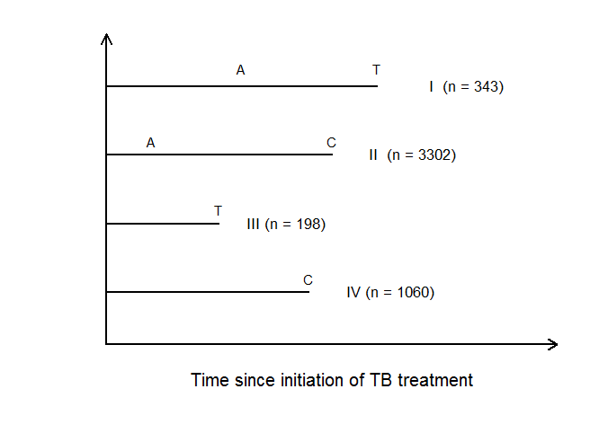
Figure 1: Patterns of observed information on ART initiation time $A$ and death time $T$. Either or both may be right censored prior to one year at time $C$.

To address these issues, we formulate a structural causal hazard model that captures the effects of both timing and duration of ART on hazard of mortality using unspecified smooth functions, and we derive methods for generating consistent estimates of model parameters under nonrandom treatment allocation and complex censoring patterns. Using output from the fitted model, we generate estimates of the functional causal relationship between ART timing and mortality. Our method can be used to estimate the survival distribution — and therefore any functional of the survival distribution — associated with any specific ART initiation time. Our analyses of the AMPATH data uses one-year survival as the primary endpoint because it is consistent with one of the major randomized trials (Havlir et al., 2011), but any functional of the survival distribution could be used.

This paper is organized as follows: the remainder of Section 1 provides additional background on issues related to HIV/TB co-infection and reviews statistical approaches related to estimating causal effect of treatment timing. Section 2 describes notation, defines optimal initiation time, and provides detailed specification of our marginal structural proportional hazards model. Section 3 develops the methods for fitting the model to observational data where both treatment timing and death time are subject to censoring. Section 4 presents results from applying our analysis of AMPATH data, with emphasis on new insights that can be gained, relative to findings from randomized trials. Section 5 summarizes a simulation study that examines properties of model-based inferences. In Section 6 we put the results in context by comparing them with RCT findings and current treatment guidelines, and outline directions for further research.

1.2 Treatment of Individuals Co-infected with HIV and Tuberculosis

Generally, treatment of TB itself is a 6-month regimen. The World Health Organization (WHO) recommends that TB treatment should be initiated first, with ART initiated within the first 8 weeks for all patients and within the first 2 weeks for those with CD4 less than 50. However, complications associated with early initiation of ART may discourage treatment adherence and cause adverse effects resulting from drug interactions and IRIS (WHO, 2013).

Recent RCTs provide an evidence base for these recommendations. For brevity, ART initiation time is hereafter defined relative to the start of TB treatment, and measured in weeks. The AACTG study A5221 found reduced 48-week mortality in the CD4$<$50 subgroup, comparing the early ($0-2$) to the late ($8-12$) initiation arm (Havlir et al., 2011). The SAPIT trial recorded significantly higher mortality rate for the initiating interval $24-28$ compared to $0-4$ or $8-12$ (Abdool Karim et al., 2011). In the CAMELIA trial, significantly reduced hazard of death was found in the early initiation arm (2 versus 8) (Blanc et al., 2011).

The question of ART timing has also been examined in at least three observational studies. An analysis of 322 co-infected patients from Spain showed longer survival for those starting ART in the first 2 months of TB treatment, compared to 3 months (Velasco et al., 2009). A prospective cohort study of 667 individuals in Thailand demonstrated an increased risk of death with longer delays in ART initiation (Varma et al., 2009). An analysis of 308 co-infected adults in Rwanda concluded that early ART initiation reduced mortality in persons with CD4 count below 100 (Franke et al., 2011).

1.3 Data Source: AMPATH Medical Record System (AMRS)

AMPATH provides care to over 160,000 HIV-positive individuals at 143 sites in western Kenya. The AMPATH Medical Record System (AMRS), one of the largest of its kind in sub-Saharan Africa, contains more than 100 million clinical observations from over 300,000 enrolled patients (Rachlis et al., 2015). Our analysis makes use of clinical encounter data from 4903 adults with HIV/TB co-infection drawn from the AMRS between March 1, 2004 and April 18, 2008. The dataset contains individual-level information at baseline on the following variables: age, gender, WHO stage (a 4-level ordinal diagnostic indicator of HIV severity), weight, CD4 count, clinic visit (urban versus rural), marital status and post-primary education. The dataset includes also longitudinal information on ART initiation status, death, and CD4 count. Among all patients presenting with HIV/TB co-infection, 26% have incomplete information on ART initiation time (case III and IV in Figure 1).

These data were generated before the findings from the studies referenced above were released; this, combined with the exercise of clinical judgment in making treatment decisions, yields significant variation in ART initiation time, even among those whose clinical profiles are similar in terms of recorded information.

1.4 Statistical Methods for Treatment Duration and Timing

Our methods address inference about causal effect of treatment initiation time on a survival distribution. The related problem of causal effect of treatment duration (assuming initiation time is the same for everyone) has been investigated in two papers by Johnson and Tsiatis (2004, 2005); the first considers the case where duration is discrete and the second extends to the more complex case of continuous time. In both cases, duration time is subject to censoring that may be related to measured covariates, and inverse probability weighting is used to address nonrandom treatment allocation. Both papers restrict attention to the mean or regression function related to a single endpoint; in our setting, we use survival time as the endpoint, which introduces the need to deal with censoring of both the exposure and the endpoint. Our approach to inference builds on Johnson and Tsiatis (2004, 2005), particularly as it relates to the use of a Radon-Nikodym derivative for deriving appropriate weight functions (see also Murphy et al., 2001). Work by Xiao et al. (2014) uses regression splines to model the weighted sum of treatment duration and estimate the effect of cumulative exposure to ART. Our model includes a term for treatment duration as a function of time, separately captures effect of timing, and allows the effect of duration to depend on timing (provided sufficient data are available).

The analysis by Franke et al. (2011), referenced above, uses a model that has a similar formulation to ours. They use pooled logistic regression with inverse probability weights to fit a marginal structural model to a sample from 308 individuals. Our paper formalizes that approach for continuous-time settings and considerably relaxes distributional assumptions about the underlying potential outcomes distributions.

The fitted model can be used to estimate the entire distribution of potential outcomes corresponding to a given initiation time. The estimated causal relationships are highly data-driven in the sense that key parts of the structural model are left unspecified, including the baseline hazard function, the instantaneous effect of treatment as a function of initiation time, and the effect of treatment duration once initiated. The added versatility of our model is motivated by the desire to take full advantage of the information available in our much larger cohort (which, to our knowledge, is larger than any cohort associated with a published analysis on HIV/TB co-infection).

2 Formulation of Potential Outcomes Model

2.1 Notation for Potential Outcomes and Observed Data

Let $t$ denote time elapsed from the initiation of TB therapy, and let $t_{\rmn{max}}$ denote maximum follow-up time. Let $T_{a}>0$ denote the potential outcome corresponding to time of death under the scenario that ART is initiated at time $a$, where $a\geq 0$ is continuous. We use $T_{\infty}$ to denote death time corresponding to any $a>t_{\rmn{max}}$.

Information on potential outcomes is observed according to the cases depicted in Figure 1. Let $A$ be the random variable representing ART initiation time and let $T=T_{A}$ denote the survival time corresponding to initiating ART at $A$. Let $C$ denote a censoring time. As shown in Figure 1, either or both of $A$ and $T_{A}$ may be right censored, for example due to loss to follow up. The observed data available for drawing inference about the distribution of potential outcomes are as follows: the observed follow up time for the mortality outcome is $T^{*}=\min(T,C)$, with event indicator $\Delta^{T}=I(T<C)$. Similarly, the observed follow up time for ART initiation time is $A^{*}=\min(A,T^{*})=\min(A,T,C)$, with event indicator $\Delta^{A}=I(A<T^{*})$. Notice that $A$ can be right censored by $T$, as shown in Case II of Figure 1. Because large ART initiation times are infrequently observed in our data, we administratively censor $A$ and $T^{*}$ at $t_{\rmn{max}}$ for cases where $A\geq t_{\rmn{max}}$ and $T^{*}>t_{\rmn{max}}$, respectively.

Each individual has $p$ covariates, some of which may be time varying. We use $L(t)$, $t\geq 0$ to denote the $p\times 1$ vector containing the most recently observed value of each covariate at time $t$, with $\overline{L}(t)=\{L(s):0\leq s<t\}$ representing the observed covariate history up to but not including $t$. For each individual, therefore, we observe a copy of $\left\{\overline{L}(A^{*}),T^{*},\Delta^{T},A^{*},\Delta^{A}\right\}$. The letter $A$ was originally used for AZT (zidovudine) and $L$ for lymphocyte cell count in earlier causal inference literature (Miguel Hernan, personal communication).

2.2 Marginal Structural Model for Mortality

We assume $T_{a}$ follows a marginal structural proportional hazards model of the form

$$\lambda_{a}(t) = \lambda_{\infty}(t)\;r(t,a),$$ (1)

where $\lambda_{a}(t)$ is the hazard function for $T_{a}$, $\lambda_{\infty}(t)$ is the reference hazard for $T_{\infty}$, and $r(t,a)>0$ is the (time-dependent) hazard ratio function. We parameterize $r(t,a)$ in terms of three functions, $g_{1}(a)$, $g_{2}(t-a)$ and $g_{3}(a(t-a))$, respectively denoting effects of timing, duration, and timing-duration interaction. Specifically, we assume

$$r(t,a) = \exp\left[I(a<t)\left\{g_{1}(a)+g_{2}(t-a)+g_{3}(a(t-a))\right\}\right],$$ (2)

where $g_{1}(\cdot)$, $g_{2}(\cdot)$ and $g_{3}(\cdot)$ are unspecified smooth functions that are twice continuously differentiable, with the second derivative set to zero at the interval boundaries for $a$, $t-a$ and $a(t-a)$. The hazard function $\lambda_{a}(t)$ can depend on baseline covariates $L(0)$ by elaborating model (2) or by using a stratified version of $\lambda_{\infty}(t)$, as demonstrated in Section 4.

The model can be understood by considering some simple cases. Figure 2 illustrates three simplified versions of the hazard model and the corresponding survival models. For clarity, models in Figure 2 assume $\lambda_{\infty}(t)$ is constant (our model allows it to remain unspecified) and assumes $g_{3}(a(t-a))=0$ (no interaction between $a$ and $t-a$). In Figure 2(a), we set $g_{1}(a)=\beta_{1}$ and $g_{2}(t-a)=0$, which implies the log hazard of mortality is $\log\{\lambda_{\infty}(t)\}$ prior to treatment initiation ($t<a$) and $\beta_{1}+\log\{\lambda_{\infty}(t)\}$ thereafter ($t\geq a$). This version assumes the instantaneous effect of initiating ART on hazard of mortality is not a function of initiation timing. In Figure 2(b), we allow $g_{1}(a)$ to vary with $a$, so that the effect of ART initiation does depend on its timing. In Figure 2(c), we additionally set $g_{2}(t-a)=(t-a)\beta_{2}$, where $\beta_{2}$ is a scalar, which implies that the instantaneous effect of initiating ART is $g_{1}(a)$, and that the effect of being on ART at any given time $t$ depends on duration.

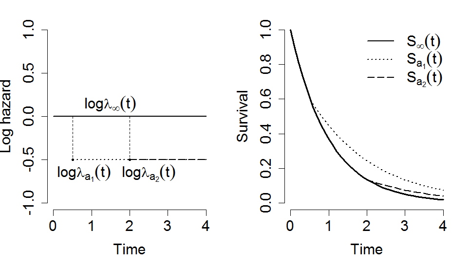
(a) $g_{1}(a_{1})=g_{1}(a_{2})=-.5;\;g_{2}(a)=0$

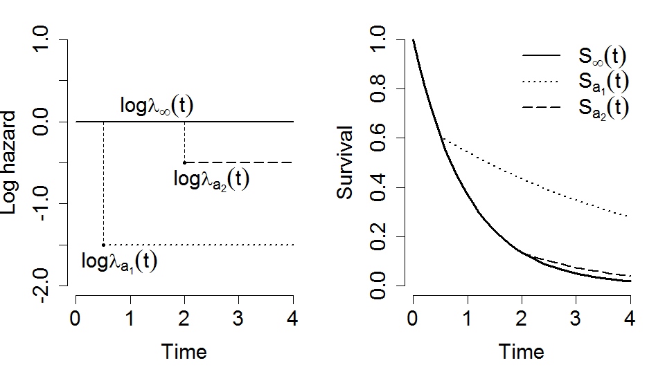
(b) $g_{1}(a_{1})=-1.5;\;g_{1}(a_{2})=-.5;\;g_{2}(a)=0$

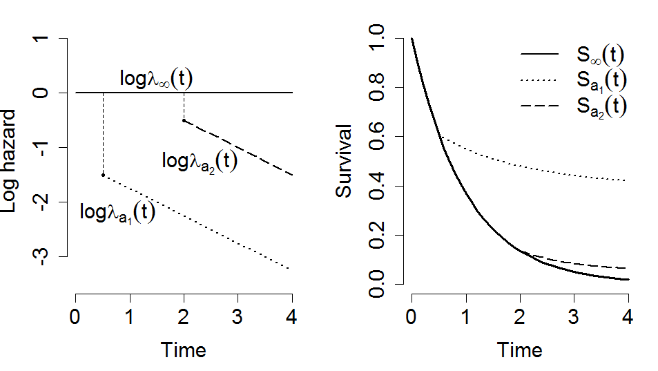
(c) $g_{1}(a_{1})=-1.5;\;g_{1}(a_{2})=-.5;\;g_{2}(a)=-.5(t-a)$

Figure 2: Simple examples of the hazard models and corresponding survival models; Two initialization times are compared: $a_{1}=.5;\;a_{2}=2.$

Turning to the more general formulation, we parameterize $g_{1}(\cdot)$, $g_{2}(\cdot)$ and $g_{3}(\cdot)$ using natural cubic splines constructed from piecewise third-order polynomials that pass through a set of control points, or knots. A natural cubic spline has continuous first and second derivatives at the knots, and is linear beyond the boundary knots. Basis functions generated under these constraints are called B-spline functions (Hastie et al., 2009). Parameterizing (2) in terms of B-splines yields

$$\lambda_{a}(t) = \lambda_{\infty}(t)\exp\left[I(a<t)\left\{b_{1}^{\top}(a)\beta_{1}+b_{2}^{\top}(t-a)\beta_{2}+b_{3}^{\top}(a(t-a))\beta_{3}\right\}\right],$$ (3)

where $b_{1}(\cdot)=(b_{\!{}_{11}}(\cdot),\ldots,b_{\!{}_{1K_{1}}}(\cdot))^{\top}$ is a $K_{1}\times 1$ vector representing a B-spline basis function of degree $K_{1}$ in $a$, and $b_{2}(\cdot)=(b_{\!{}_{21}}(\cdot),\ldots,b_{\!{}_{2K_{2}}}(\cdot))^{\top}$ and $b_{3}(\cdot)=(b_{\!{}_{31}}(\cdot),\ldots,b_{\!{}_{3K_{3}}}(\cdot))^{\top}$, having dimension $K_{2}\times 1$ and $K_{3}\times 1$, respectively, are defined similarly as functions of $t-a$ and $a(t-a)$. The parameters $\beta_{1}$, $\beta_{2}$ and $\beta_{3}$ are, respectively, $K_{1}\times 1$, $K_{2}\times 1$ and $K_{3}\times 1$ vectors of coefficients for the basis functions $b_{1}(\cdot)$, $b_{2}(\cdot)$ and $b_{3}(\cdot)$. The model for the risk function can be written in compact form as $r(t,a)=\exp\{X^{\top}(a,t)\beta\},$ where

$$X(a,t)~\!{}_{(K_{1}+K_{2}+K_{3})\times 1}=I(a<t)[b_{1}^{\top}(a),b_{2}^{\top}(t-a),b_{3}^{\top}(a(t-a))]^{\top}$$ (4)

and $\beta~\!{}_{(K_{1}+K_{2}+K_{3})\times 1}=(\beta_{1}^{\top},\beta_{2}^{\top},\beta_{3}^{\top})^{\top}$. The causal effect of ART initiation time on the survival distribution is therefore encoded in $\beta$, and the formulation in terms of B-spline basis functions allows the use of weighted proportional hazards regression methods to obtain consistent estimates of $\beta$.

3 Estimation of Structural Model and Optimal Initiation Time

3.1 Overview

In our data, the decision to initiate ART depends on information available to the physician, and is therefore not randomly allocated. Moreover, $A$ will be right censored when an individual dies or leaves the study before treatment initiation. We propose to estimate $\beta$ by maximizing an inverse-probability-weighted partial likelihood score function. We show how to construct and estimate weights that lead to consistent estimates of $\beta$ under specific assumptions about treatment allocation and censoring, and in Web Appendix Section 1, we provide a heuristic justification based on the use of Radon-Nikodym derivatives (Murphy et al., 2001).

In deriving the weighted estimating equations for $\beta$, we first consider the hypothetical case where $A$ is not randomized and where $T$ is always observed. Next, we move to the case where $A$ may be censored by $T$ (i.e., where death occurs prior to treatment initiation), but there is no censoring by $C$. We then describe the case where $A$ is not randomized, and possibly censored by $T$. Finally, we generalize our approach to allow for censoring by $C$. We then show how to construct causal contrasts between different treatment initiation times using output from the fitted model.

3.2 Randomized Treatment Assignment

If treatment is randomly allocated according to a known probability density $f^{A}(\cdot)$, we can use the standard partial likelihood score equations to derive consistent estimators of $\beta$. For this simple case we assume $A$ is observed for everyone and there is no censoring by $C$. For $t>0$, let $N^{T}(t)=I\left\{T\leq t,\Delta^{T}=1\right\}$ denote the zero-one counting process associated with $T$. Let $Y(t)=1$ if an individual is still at risk for death and under observation at $t$, and $Y(t)=0$ otherwise. The partial likelihood score equations can be written $\sum_{i=1}^{n}D_{i}(\beta)=0$, where

$$D_{i}(\beta) = D(A_{i},T_{i};\beta)$$ (5)

$$= \int_{0}^{\infty}\left\{X(A_{i},t)-\overline{X}(t,\beta)\right\}dN^{T}_{i}(t),$$

where $X(A_{i},t)$ is the design matrix based on (4) and

$$\overline{X}(t,\beta) = \frac{\sum_{k}X(A_{k},t)Y_{k}(t)r(A_{k},t;\beta)}{\sum_{k}Y_{k}(t)r(A_{k},t;\beta)}.$$

Let $E_{R}(\cdot)$ denote expectation under randomized treatment assignment. Under randomization of $A$, $n^{-1}\sum_{i}D(A_{i},T_{i};\beta)$ is an unbiased estimator of $E_{R}\left\{D(A,T;\beta)\right\}$. The estimating function $\sum_{i}D_{i}(\beta)$ is a stochastic integral of a predictable process with respect to a martingale, and as such $E_{R}\left\{D(A,T;\beta_{0})\right\}=0$ at the true value $\beta_{0}$ of $\beta$; hence, the root $\widehat{\beta}$ of the estimating equation $\sum_{i=1}^{n}D_{i}(\beta)=0$ is a consistent estimator of $\beta$ (Fleming and Harrington, 2005, pp. 297-298).

Now consider the case where $A$ is still randomly allocated, but death may occur before initiation of treatment, so that $A^{*}=\min(A,T)$ and $\Delta^{A}=I(A<T)$. We continue to assume no censoring by $C$. Following Johnson and Tsiatis (2005), the mean of an individual score contribution can be represented as the sum of contributions from those with observed and censored values of $A$; i.e., $E_{R}\left\{D(A_{i},T_{i};\beta)\right\}=E_{R}\left\{\Delta^{A}_{i}D(A_{i},T_{i};\beta)+(1-\Delta^{A}_{i})D(A_{i},T_{i};\beta)\right\}$. Contributions corresponding to censored values of $A$ have expectation

$$E_{R}\left\{(1-\Delta^{A}_{i})D(A_{i},T_{i};\beta)\right\} = E_{R}\left[E_{R}\left\{(1-\Delta^{A}_{i})D(A_{i},T_{i};\beta)\,\left|\,\Delta^{A}_{i},A^{*}_{i}\right.\right\}\right]$$ (6)

$$= E_{R}\left[(1-\Delta^{A}_{i})E_{R}\left\{D(A_{i},T_{i};\beta)\,\left|\,\Delta^{A}_{i},A^{*}_{i}\right.\right\}\right]$$

$$= E_{R}\left\{(1-\Delta^{A}_{i})\int_{A^{*}_{i}}^{\infty}D(a,T_{i},\beta)dF^{A{\,|\,}A>A^{*}_{i}}(a)\right\}$$

$$= E_{R}\left\{\frac{(1-\Delta^{A}_{i})}{1-F^{A}(A^{*}_{i})}\int_{A^{*}_{i}}^{\infty}D(a,T_{i},\beta)dF^{A}(a)\right\}.$$

To evaluate (6), note that $D(a,T_{i};\beta)=\int_{0}^{\infty}\{X(a,t)-\overline{X}(t,\beta)\}dN^{T}_{i}(t)$, and recall that $X(a,t)=I(a<t)[b_{1}^{\top}(a),b_{2}^{\top}(t-a),b_{3}^{\top}(a(t-a))]^{\top}$, so that $X(a,t)=0$ for $a\geq t$. This implies $D(a,T_{i},\beta)$ is a constant function of $a$, with $D(a,T_{i},\beta)=-\overline{X}(T_{i},\beta)$ for $a\geq A_{i}^{*}$ and 0 otherwise. The integral in (6) therefore reduces to $-\overline{X}(T_{i},\beta)\{1-F^{A}(A^{*})\}$, and the expectation itself reduces to $E_{R}\left\{-(1-\Delta^{A}_{i})\overline{X}(T_{i},\beta)\right\}$.

Pulling this all together, we see that when death may occur before treatment initiation, and when there is no censoring by $C$, $n^{-1}\sum_{i}D_{i}(\beta)$ is an unbiased estimator of
$E_{R}\left\{\Delta^{A}D(A,T;\beta)-(1-\Delta^{A})\overline{X}(T,\beta)\right\}$, which implies that the solution $\widehat{\beta}$ to the modified estimating equations

$$\sum_{i=1}^{n}\left\{\Delta_{i}^{A}D(A_{i},T_{i};\beta)-(1-\Delta_{i}^{A})\overline{X}(T_{i},\beta)\right\} = 0$$ (7)

will yield a consistent estimator of $\beta$.

3.3 Non-random Allocation of Treatment

Suppose now that $A$ is not randomly allocated, but that treatment allocation can be considered ignorable in the sense that

$$\lambda^{A}(t{\,|\,}\overline{L}(t),\mathscr{T}_{\{a\geq t\}}) = \lambda^{A}(t{\,|\,}\overline{L}(t)),$$ (8)

where $\mathscr{T}_{\{a\geq t\}}=\{T_{a}:a\geq t\}$ is the set of potential failure times associated with initiation times beyond $t$. This assumption states that initiation of treatment at time $t$ is sequentially randomized in the sense that it is independent of future potential outcomes, conditionally on observed covariate history $\overline{L}(t)$ (Robins, 1999).

Let $\mathbb{P}_{R}(\cdot)$ denote the data distribution under randomized treatment, and let $\mathbb{P}_{O}(\cdot)$ denote the same under non-random allocation of treatment. Recall that the observable data for each individual, under either randomized or non-randomized allocation of treatment, is $\{A^{*},\Delta^{A},T^{*},\Delta^{T}\}$. Following Murphy et al. (2001) and Johnson and Tsiatis (2005), under the sequential randomization assumption in (8) and some regularity conditions, including the positivity assumption referenced in Web Appendix Section 1, the distribution of $\{A^{*},\Delta^{A},T^{*},\Delta^{T}\}$ under $\mathbb{P}_{R}(\cdot)$ is absolutely continuous with respect to the distribution of $\{A^{*},\Delta^{A},T^{*},\Delta^{T}\}$ under $\mathbb{P}_{O}(\cdot)$, and a version of the Radon-Nikodym (R-N) derivative is

$$E_{O}\left\{\left.\frac{\Delta^{A}\,f^{A}(A^{*})}{f^{A}(A^{*}{\,|\,}\overline{L}(A^{*}))}+\frac{(1-\Delta^{A})(1-F^{A}(A^{*}))}{1-F^{A}(A^{*}{\,|\,}\overline{L}(A^{*}))}\,\right|\,A^{*}=a,\Delta^{A}=\delta^{A},T^{*}=t,\Delta^{T}=\delta^{T}\right\}.$$ (9)

An estimating equation that is a function of observed data and is unbiased under the distribution of $\mathbb{P}_{R}(\cdot)$ can be re-weighted by the R-N derivative to obtain an unbiased estimating equation using the same observed data, but now under the distribution $\mathbb{P}_{O}(\cdot)$ (Murphy et al., 2001). Define weights $W_{1i}^{A}$ and $W_{2i}^{A}$ as

$$W_{1i}^{A}(t) = \frac{f^{A}(t)}{f^{A}(t{\,|\,}\overline{L}_{i}(t))},\;\;\;W_{2i}^{A}(t)\;=\;\frac{1-F^{A}(t)}{1-F^{A}(t{\,|\,}\overline{L}_{i}(t))}.$$

The R-N derivative in (9) suggests using the weighted estimating equation

$$\sum_{i=1}^{n}\Delta_{i}^{T}\left\{\Delta_{i}^{A}D^{*}(A_{i},T_{i};\beta)W_{1i}^{A}(A_{i})-(1-\Delta_{i}^{A})\overline{X}^{*}(T_{i};\beta)W_{2i}^{A}(T_{i})\right\} = 0,$$ (10)

where $D^{*}$ and $\overline{X}^{*}$ are evaluated using weighted risk set indicators

$$Y^{*}_{i}(t) = Y_{i}(t)\left\{I(A_{i}<t)W_{1i}^{A}(A_{i})+I(A_{i}\geq t)W_{2i}^{A}(t)\right\}.$$

Up to now we have assumed no censoring by $C$. Let $N^{A}(t)=I\{A\leq t,\Delta^{A}=1\}$, for $t>0$, denote the zero-one counting process for treatment initiation, with $\overline{N}^{A}(t)$ representing treatment history information up to time $t$. Similarly, define $N^{C}(t)=I(C\leq t,\Delta^{T}=0)$. We assume that censoring at $t$ can depend on covariate and treatment history, but conditionally on these is independent of future potential outcomes. This assumption can be expressed formally in terms of the hazard function associated with $N^{C}(t)$,

$$\lambda^{C}(t{\,|\,}\overline{N}^{A}(t),\;\overline{L}(t),\;\mathscr{T}_{\{a\geq t\}}) = \lambda^{C}(t{\,|\,}\overline{N}^{A}(t),\;\overline{L}(t)).$$ (11)

As with the treatment initiation process, we can define a weight function associated with censoring,

$$W^{C}_{i}(t) = \frac{1-F^{C}(t)}{1-F^{C}(t{\,|\,}\overline{N}^{A}(t),\overline{L}_{i}(t))}.$$

This leads to a final modification of the estimating equations for $\beta$ to accommodate covariate- and treatment-dependent censoring,

$$U_{n}(\beta) = \sum_{i=1}^{n}\Delta_{i}^{T}~{}W^{C}_{i}(T_{i})\left\{\Delta_{i}^{A}D^{**}(A_{i},T_{i};\beta)W_{1i}^{A}(A_{i})-(1-\Delta_{i}^{A})\overline{X}^{**}(T_{i};\beta)W_{2i}^{A}(T_{i})\right\},$$ (12)

where $D^{**}$ and $\overline{X}^{**}$ are evaluated using weighted risk set indicators

$$Y^{**}_{i}(t) = Y_{i}(t)\,W_{i}^{C}(t)\left\{I(A_{i}<t)W_{1i}^{A}(A_{i})+I(A_{i}\geq t)W_{2i}^{A}(t)\right\}.$$

Writing (12) in terms of counting process notation used in (5) makes the distinct contributions of the four observation patterns in Figure 1 more transparent,

$$U_{n}(\beta) = \sum_{i=1}^{n}\int_{0}^{\infty}W^{C}_{i}(t)\left[\Delta_{i}^{A}\,W_{1i}^{A}(A_{i})\left\{X(A_{i},t)-\overline{X}^{**}(t;\beta)\right\}-(1-\Delta_{i}^{A})\,W_{2i}^{A}(t)\,\overline{X}^{**}(t;\beta)\right]dN_{i}^{T}(t).$$

In particular all individuals censored by $C$, either before or after initiating treatment (cases II and IV in Figure 1), contribute information about $\beta$ via contributions to the risk set up to the observed censoring time $C$.

3.4 Estimation of the Weights

The weights in (12) depend on the marginal and conditional density functions of $A$ and $C$, which can be estimated from fitted models of the marginal and conditional intensity processes associated with $N^{A}(t)$ and $N^{C}(t)$. To estimate $f^{A}(t{\,|\,}\overline{L}(t))$, we assume $\lambda^{A}(t{\,|\,}\overline{L}(t))$ follows a proportional hazards regression parameterized using a finite-dimensional parameter $\alpha^{A}$,

$$\lambda^{A}(t{\,|\,}\overline{L}(t)) = \lambda_{0}^{A}(t)\,r^{A}(\overline{L}(t);\,\alpha^{A}),$$ (13)

where $r$ is a user-specified regression function. (We use a proportional hazards formulation for convenience, but any regression formulation can be used here). The conditional density function $f^{A}(t{\,|\,}\overline{L}(t))$ can be estimated using the empirical cumulative hazard,

$$\Lambda^{A}(t{\,|\,}\overline{L}(t),\widehat{\alpha}^{A}) = \int_{0}^{t}\dfrac{r^{A}(L(s);\,\widehat{\alpha}^{A})dN(s)}{\sum_{j}Y_{j}(s)r^{A}(L(s);\,\widehat{\alpha}^{A})}$$

$$1-F^{A}(t{\,|\,}\overline{L}(t),\widehat{\alpha}^{A}) = \exp\left\{-\Lambda^{A}(t{\,|\,}\overline{L}(t),\widehat{\alpha}^{A})\right\},$$

$$\widehat{f}^{A}(t{\,|\,}\overline{L}(t)) = \lambda^{A}(t{\,|\,}\overline{L}(t),\widehat{\alpha}^{A})\left\{1-F^{A}(t{\,|\,}\overline{L}(t),\widehat{\alpha}^{A})\right\},$$

where $\widehat{\alpha}^{A}$ is the maximum partial likelihood estimator for model (13).

To estimate the unknown marginal probability density $f^{A}(t)$, we use the Nelson-Aalen estimator $\widehat{\Lambda}^{A}(t)=\sum_{i}\int_{0}^{t}\,dN_{i}^{A}(s)/Y_{i}(s)$ for the cumulative hazard function and $\widehat{\lambda}^{A}(t)=d\widehat{\Lambda}^{A}(t)$ for the hazard function. The estimated CDF and density functions are obtained using $\widehat{F}^{A}(t)=1-\exp\{-\widehat{\Lambda}^{A}(t)\}$ and $\widehat{f}^{A}(t)=\widehat{\lambda}^{A}(t)\{1-\widehat{F}^{A}(t)\}$, respectively. The weight estimators are therefore a function of $\widehat{F}^{A}$, $\widehat{f}^{A}$, and $\widehat{\alpha}^{A}$,

$$\widehat{W}_{1i}^{A}(t) = \frac{\widehat{f}^{A}(t)}{\widehat{f}^{A}(t{\,|\,}\overline{L}_{i}(t))},\;\;\;\widehat{W}_{2i}^{A}(t)\;=\;\frac{1-\widehat{F}^{A}(t)}{1-F^{A}(t{\,|\,}\overline{L}_{i}(t),\widehat{\alpha}^{A})}.$$

The weights $W_{i}^{C}(t)$ can be estimated in a similar fashion by specifying and fitting a regression model of the form $\lambda^{C}(t{\,|\,}\overline{N}^{A}(t),\,\overline{L}(t))=\lambda_{0}^{C}(t)\,r^{C}(\overline{N}^{A}(t),\,\overline{L}(t),\,\alpha^{C})$ to obtain estimates of $f^{C}(t{\,|\,}\overline{N}^{A}(t),\overline{L}(t))$ and $F^{C}(t{\,|\,}\overline{N}^{A}(t),\overline{L}(t))$, and using the Nelson-Aalen estimator
$\widehat{\Lambda}^{C}(t)=\sum_{i}{\int_{0}^{t}}\,dN_{i}^{C}(s)/Y_{i}(s)$ to obtain estimates of $f^{C}(t)$ and $F^{C}(t)$.

3.5 Optimal Initiation Time

Referring back to our structural hazard model (2), the survival function for the potential outcome $T_{a}$ corresponding to initiation time $a$ is $S_{a}(t)=\exp\{-\Lambda_{a}(t)\}$, where

$$\Lambda_{a}(t) = I(t<a)\Lambda_{\infty}(t)$$ (14)

$$+ I(t\geq a)\left[\Lambda_{\infty}(a)+\int_{a}^{t}\exp\{g_{1}(a)+g_{2}(u-a)+g_{3}(a(u-a))\}\mathrm{d}\Lambda_{\infty}(u)\right].$$

The $g$ functions are estimated using weighted partial likelihood score as described above, and the baseline cumulative hazard $\Lambda_{\infty}(t)$ is estimated using the (weighted) Breslow estimator that arises from the fitting process. The survivor function $S_{a}(t)$ can therefore be estimated for any combination of $a$ and $t$, enabling estimation of specific causal contrasts such as mortality ratios $S_{a}(t)/S_{a^{\prime}}(t)$ for $a\neq a^{\prime}$.

With sufficient amounts of data, we also can use model output to infer optimal timing for treatment initiation. An optimal initiation time is defined as the value of $a$ that maximizes an objective function written in terms of a functional of the distribution of potential outcomes. Specifically, let $F_{a}(t)=P(T_{a}\leq t)$ denote the CDF associated with $T_{a}$, and let $\theta_{a}=\theta(F_{a})$ denote a scalar functional of $F_{a}$ (e.g., the mean $\int t\;dF_{a}(t)$ or median $F_{a}^{-1}({\textstyle\frac{1}{2}})$). For a given functional $\theta_{a}$, the optimal initiation time is $a_{\text{opt}}=\arg\max_{a}\theta_{a}$.

In our application we use one-year survival $\theta_{a}=1-F_{a}(t_{0})$, with $t_{0}$ set to 52 weeks, as the primary endpoint. Our estimates of $a_{\text{opt}}$ were somewhat unstable because the one-year mortality curve as a function of initiation time appears to be monotone increasing from zero (i.e., nonconvex). Alternatively, we compare mortality rates for contextually motivated initiation time intervals (trials referenced in Section 1) to draw inferences about optimal timing. We elaborate in Section 4.

4 Application to AMPATH data

Our analysis dataset contains 4903 HIV/TB co-infected patients who had TB therapy initiated and had a CD4 count below 350 at the start of TB therapy. Under guidelines in place at the time, these patients were eligible for ART initiation. Baseline ($t=0$) is defined as the time of TB treatment initiation. The total number of deaths is 541. To avoid influence of sparsely distributed large values of ART initiation times, we administratively censor the data at 1.5 years ($t_{\text{max}}$). Of the 3302 patients in case II and 1060 patients in case IV of Figure 1, 1335 and 38 were administratively censored at $t_{\text{max}}$, respectively.

At the time when these data were collected, baseline CD4 was a key marker used to decide ART initiation time. To be consistent with AMPATH guidelines, we divide baseline CD4 count into groups defined by the intervals $[0,50]$, $(50,200]$, $(200,350]$. Median weeks to ART initiation is 4 for CD4 $\leq$ 50, 8 for CD4 $\in(50,200]$ and 12 for CD4 $\in(200,350]$.

Baseline covariates and time-varying CD4 count (1.9 CD4 measures per year per person) were used to fit the hazard models $\lambda^{A}(t{\,|\,}\overline{L}(t))$ and $\lambda^{C}(t{\,|\,}\overline{N}^{A}(t),\overline{L}(t))$ leading to treatment and censoring weights. Each model included the main effect of each covariate; higher-order polynomial terms for continuous variables were tested and found not to add information. Estimated model coefficients are summarized in Web Table 2. Bootstrap re-sampling with 1000 replicates is used to estimate standard errors of the estimated mean one-year survival; censoring and ART initiation time models are re-fit within each bootstrap sample.

All calculations are carried out in R. The hazard models for ART initiation time and censoring time are fitted using R function coxph. The structural model given by (3) is fitted using weighted partial likelihood, also using coxph (Therneau, 2015), with spline basis functions for $g_{1}(a)$, $g_{2}(t-a)$ and $g_{3}(a(t-a))$ generated using the R function ns. We place knots at the 25th, 50th and 75th percentile of the uncensored values of $A^{*}$ for $g_{1}(\cdot)$; $T^{*}-A^{*}$ for $g_{2}(\cdot)$; and $A^{*}(T^{*}-A^{*})$ for $g_{3}(\cdot)$.

In Web Appendix Section 3, we describe steps of fitting the structural model (3), show plots of each estimated $g$ function, and summarize key findings from the plots. Plots of $g$ functions for the CD$\leq$50 subgroup appear in Figure 3.

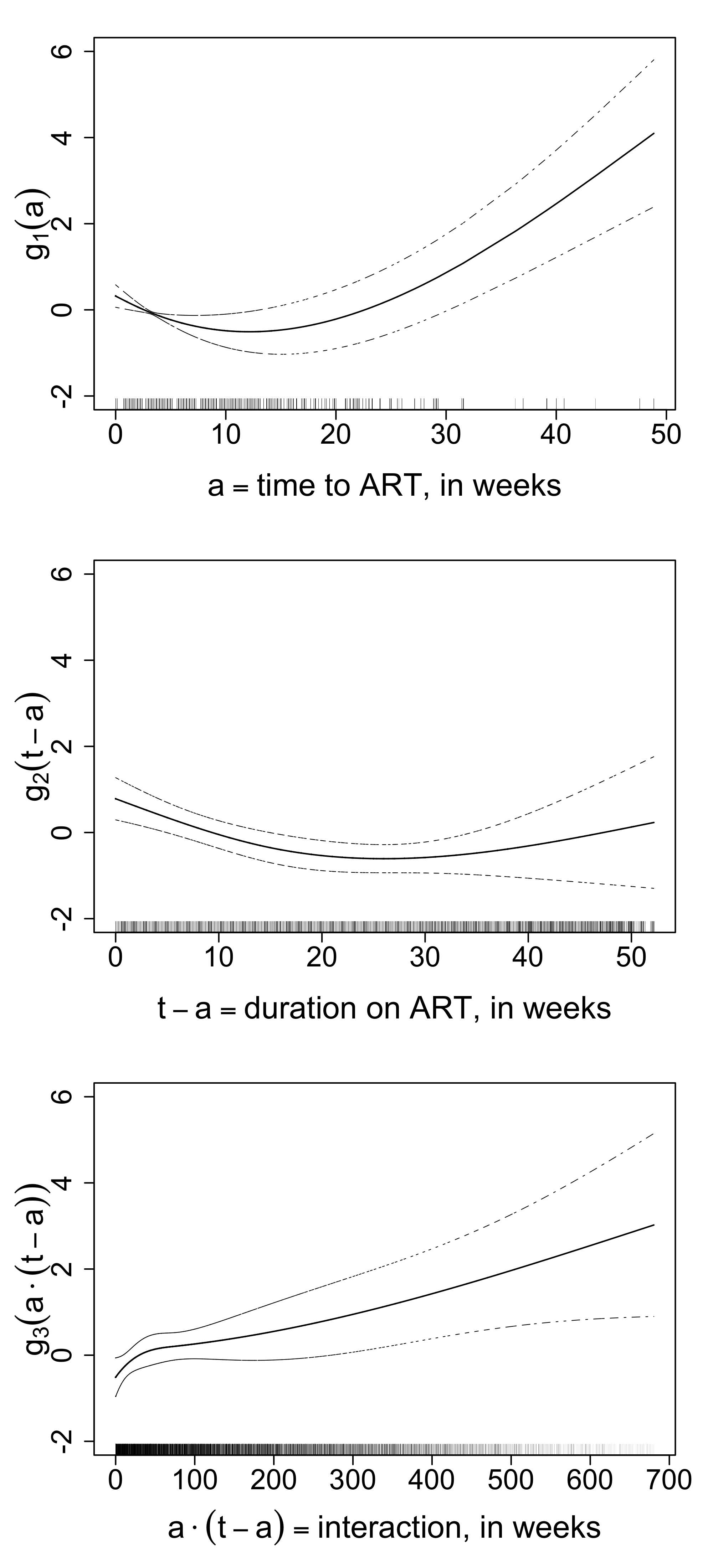
Figure 3: Fitted curves $g_{1}(a)$, $g_{2}(t-a)$ and $g_{3}(a(t-a))$, for baseline CD4$\leq$50. See model (2).

The plot of $\widehat{g}_{1}(a)$ in the first panel of Figure 3 shows that the instantaneous effect of ART initiation is U-shaped, with maximum benefit (lowest mortality hazard) just after 10 weeks, and lower effectiveness with longer delays. In the second panel, $\widehat{g}_{2}(t-a)$ depicts the effect of treatment duration, and generally indicates that longer duration times are associated with lower mortality hazard. The increasing trend in the interaction term $\widehat{g}_{3}(a(t-a))$ suggests that delayed ART initiation reduces the effect of duration on treatment. The quadratic trend in $\widehat{g}_{1}(a)$ supports the notion that immediate treatment initiation carries some risk of elevated mortality that is possibly balanced out by the benefit of remaining on treatment longer. The net causal effect is summarized in plots comparing one-year mortality rate between regimes $a$ and $a^{\prime}$, where $a=0$ and $a^{\prime}>0$ (Figure 5, described below).

Figure 4 shows estimated mortality curves, derived using (14), for selected ART initiation times $a\in\{0,8,24,\infty\}$ and stratified by baseline CD4 subgroup. Differences between these curves are causal contrasts. For each distinct value of $a$, mortality rate is clearly highest for those with baseline CD4 $\in[0,50]$. Looking within CD4 strata, comparing curves for $a=0$ and $a=8$ to those with $a>8$ suggests a benefit of early initiation for all groups, with greatest benefit for those in the lowest CD4 stratum. Figure 5 shows one-year mortality and the causal treatment effect $\widehat{S}_{a}(52)-\widehat{S}_{0}(52)$ as a function of treatment initiation time, stratified by baseline CD4 subgroup. The effect of early initiation is most pronounced for CD4 $\leq 50$. The results suggest immediate initiation for CD4$\leq 200$. Diagnostic plots suggest the model fits the data well (Web Figure 4).

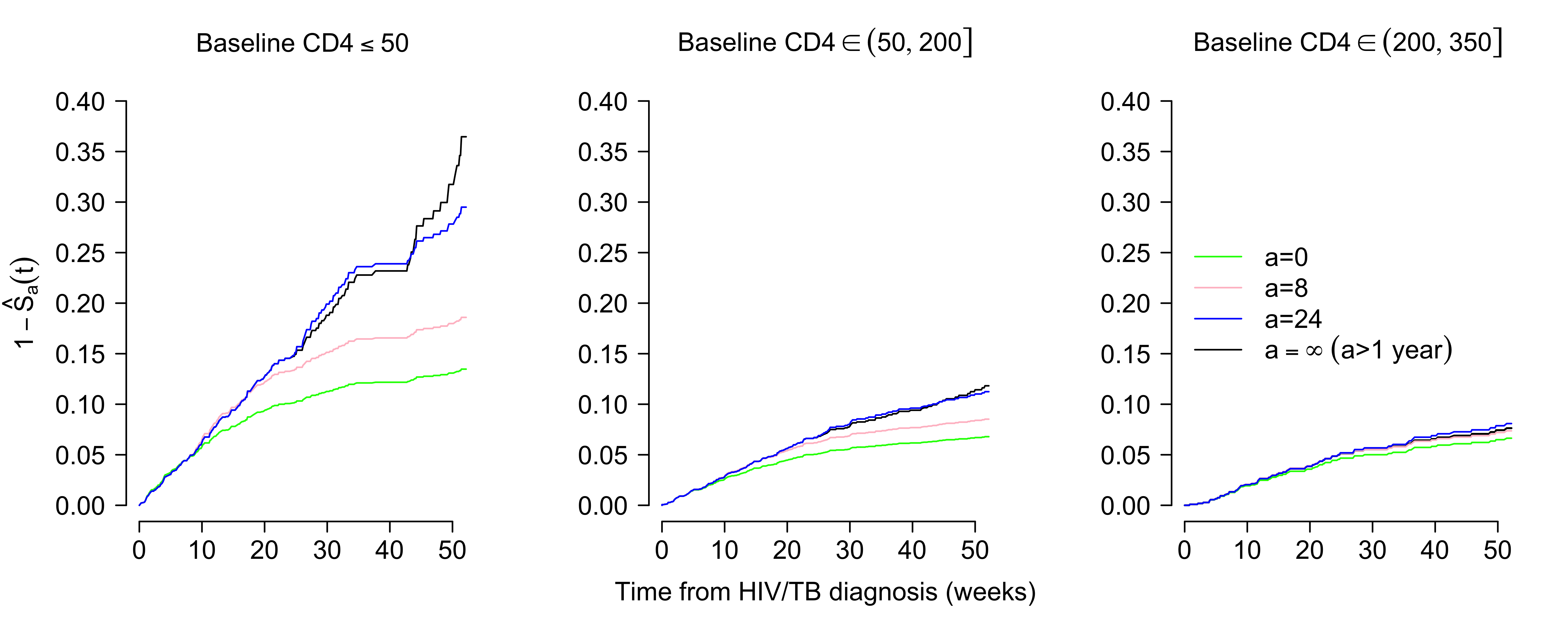
Figure 4: Estimated mortality functions $1-\widehat{S}_{a}(t)$ corresponding to ART initiation times $a\in\{0,\;8,\;24,\;\infty$}.

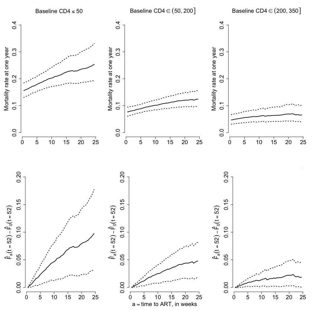
Figure 5: Top panel: causal effect of ART initiation: one-year mortality as a function of ART initiation time. Bottom panel: difference in one-year mortality between initiating ART at time $a$ and concomitant initiation with TB treatment. Stratified by baseline CD4 count.

Finally, we can emulate comparisons between regimens reported in the randomized trials cited earlier. We can mimic random allocation of treatment initiation time to specific intervals by assuming a distribution for $A$ that is independent of outcomes and covariates, and compare interval-specific mortality rates to draw inferences about treatment timing. In our data example, we assume $A$ follows a uniform distribution, and calculate one-year survival probability associated with initiating in a given interval $[t_{1},t_{2})$ via $\int_{a\in[t_{1},t_{2})}\{1-\widehat{F}_{a}(t_{0})\}dF^{U}(a)$, where $F^{U}(\cdot)$ is the CDF of the uniform distribution on $[0,t_{\text{max}}]$. To illustrate, following the SAPIT trial, we compare one-year mortality for initiating intervals $[0,4]$ and $[8,12]$ weeks. For those with CD4 $\leq 50$ ($n=1540$), our model estimated the mean mortality rate to be .16 $(.14,.19)$ for $[0,4]$ and .20 $(.17,.24)$ for $[8,12]$, with a $p$-value of .02 for the difference between the means, as compared to .10 and .20 respectively for the two regimens from the trial ($n=72$), with a $p$-value of .17 for the incidence-rate ratio.

Our results suggest ART should be initiated within 8 weeks of the initiation of TB therapy for AMPATH patients with CD4 counts lower than 200. There is a marked increase in expected one-year mortality when ART is initiated after 8 weeks (see Figure 5). For patients with CD4 $\in(200,350]$, while early initiation still results in lowest one-year mortality, there is not strong statistical evidence to support the conclusion that a specific ART initiation time (or time interval) will lead to reduced one-year mortality. Our results are consistent with AMPATH guidelines (Web Table 3) in treating HIV/TB co-infected patients, and are consistent with general findings of randomized controlled trials.

5 Simulation

We conducted a simulation to study properties of our weighted estimator when the model is correctly specified and to evaluate sensitivity of the weighted estimator to violations of the no unmeasured confounding assumption. We simulate data from a simplified version of our structural model (1). We examine bias, variability and confidence interval coverage rates related to estimates of one-year mortality for different choices of $a$ under three scenarios: 1) under random allocation of treatment; 2) with measured confounding and 3) in the presence of unmeasured confounding. The simulation results show near-zero bias and nominal coverage probability for Scenario 1. In the presence of measured confounding (Senario 2), the weighted estimator eliminates nearly all the bias and coverage probabilities are close to nominal levels as compared to the unweighted estimator. Unmeasured confounding (Scenario 3) produces bias in proportion to the degree of confounding. We provide details about the data generation algorithm, the parameter values and results in Web Appendix Section 2.

6 Summary and Discussion

Timing of ART initiation is important in HIV/TB co-infection. Determining the optimal ART initiation time is difficult because of the need to achieve balance between the risk for mortality and potential adverse events associated with early antiviral therapy initiation. Three randomized controlled trials (AACTG, SAPIT, and CAMELIA) support earlier initiation of ART for those with very low CD4 count, but initiation times are quantified on an interval scale. Our data, derived from electronic health records, allow higher-resolution inference for initiation time on a continuous scale, are sampled from a well-defined population, and reflect outcomes from actual clinical practice.

Our results are largely consistent with the findings of the clinical trials, and provide important reinforcement and elaboration of those findings. Our model provides estimates of mortality for any potential initiation time ranging from 0 to 40 weeks, and moreover it captures the separate effects of ART initiation and ART duration. This latter feature enables examination of the potential trade-offs associated with early initiation, illustrated in Figure 3. In addition to reinforcing the findings from recent trials, inference about grouped-interval-based optimal initiation times for ART are consistent with current AMPATH guidelines.

Our model assumes that both treatment initiation and censoring are independent of potential mortality outcomes, conditionally on baseline and time-dependent covariates. Given that treatment decisions are based on clinical indicators that we included in our weight model, the treatment ignorability assumption has substantive justification. It is possible that censoring could be associated with higher death rate. In the future, we will develop formal representations of potential selection biases, and use those as a basis for examining sensitivity to violations of assumptions about ignorable treatment assignment and censoring.

Our model, though flexible, can be extended in several directions. First, an important structural assumption is that the effects of initiation, duration and their interaction are additive on the log hazard scale; this requirement could be relaxed by introducing a multi-dimensional spline function. Fitting this sort of model would likely require a larger dataset. Second, our model considers regimens that are static in the sense that they are dependent on a baseline covariate (here, CD4 count). A potential topic of further research is comparison of dynamic treatment regimes, which are defined in terms of an individual’s evolving history; e.g., ‘initiate ART when CD4 first drops below $x$’ (Robins et al., 2008). Although we considered this approach, in AMPATH — as in most resource-constrained HIV care environments — data needed for these comparisons are limited because CD4 and other HIV disease markers are measured infrequently (typically every six months, but sometimes less often).

Finally, focused clinical questions that have generated considerable data from both randomized trials and observational studies are potentially fertile ground for development of new methods that combine, synthesize or compare available evidence. This activity has particular importance in the field of HIV, where large observational databases are forming the basis for important and far-reaching policy related to treatment and policy interventions (Günthard et al., 2016).

Supplementary Materials

Web Appendices, Tables, and Figures referenced in Sections 3, 4, 5, and the R code used to implement our approach are available with this paper at the Biometrics website on Wiley Online Library.

References

- Abdool Karim et al. (2010) Abdool Karim, S. S., Naidoo, K., Grobler, A., et al. (2010). Timing of initiation of antiretroviral drugs during tuberculosis therapy. New England Journal of Medicine 362, 697–706.
- Abdool Karim et al. (2011) Abdool Karim, S. S., Naidoo, K., Grobler, A., et al. (2011). Integration of antiretroviral therapy with tuberculosis treatment. New England Journal of Medicine 365, 1492–1501.
- Blanc et al. (2011) Blanc, F. X., Sok, T., Laureillard, D., et al. (2011). Earlier versus later start of antiretroviral therapy in HIV-infected adults with tuberculosis. New England Journal of Medicine 365, 1471–1481.
- Einterz et al. (2007) Einterz, R. M., Kimaiyo, S., Mengech, H. N., et al. (2007). Responding to the HIV pandemic: the power of an academic medical partnership. Academic Medicine 82, 812–818.
- Fleming and Harrington (2005) Fleming, T. R. and Harrington, D. P. (2005). Counting Processes and Survival Analysis. John Wiley & Sons, 2nd edition.
- Franke et al. (2011) Franke, M. F., Robins, J. M., Mugabo, J., et al. (2011). Effectiveness of early antiretroviral therapy initiation to improve survival among HIV-infected adults with tuberculosis: a retrospective cohort study. PLoS Medicine 8, e1001029.
- Günthard et al. (2016) Günthard, H., Saag, M., Benson, C., et al. (2016). Antiretroviral drugs for treatment and prevention of HIV infection in adults: 2016 recommendations of the International Antiviral Society–USA Panel. Journal of the American Medical Association 316, 191–210.
- Hastie et al. (2009) Hastie, T., Tibshirani, R., and Friedman, J. (2009). The Elements of Statistical Learning: Data Mining, Inference, and Prediction. Springer.
- Havlir et al. (2011) Havlir, D. V., Kendall, M. A., Ive, P., et al. (2011). Timing of antiretroviral therapy for HIV-1 infection and tuberculosis. New England Journal of Medicine 365, 1482–1491.
- Johnson and Tsiatis (2004) Johnson, B. A. and Tsiatis, A. A. (2004). Estimating mean response as a function of treatment duration in an observational study, where duration may be informatively censored. Biometrics 60, 315–323.
- Johnson and Tsiatis (2005) Johnson, B. A. and Tsiatis, A. A. (2005). Semiparametric inference in observational duration-response studies, with duration possibly right-censored. Biometrika 92, 605–618.
- Murphy et al. (2001) Murphy, S., Van Der Laan, M., and Robins, J. (2001). Marginal mean models for dynamic regimes. Journal of the American Statistical Association 96, 1410–1423.
- Rachlis et al. (2015) Rachlis, B., Ochieng, D., Geng, E., et al. (2015). Evaluating outcomes of patients lost to follow-up in a large comprehensive care treatment program in western kenya. Journal of Acquired Immune Deficiency Syndromes 68, e46.
- Robins et al. (2008) Robins, J., Orellana, L., and Rotnitzky, A. (2008). Estimation and extrapolation of optimal treatment and testing strategies. Statistics in Medicine 27, 4678–4721.
- Robins (1999) Robins, J. M. (1999). Marginal structural models versus structural nested models as tools for causal inference. Statistical Models in Epidemiology, the Environment and Clinical Trials 116, 95–133.
- Therneau (2015) Therneau, T. M. (2015). A Package for Survival Analysis in S. version 2.38.
- Varma et al. (2009) Varma, J. K., Nateniyom, S., Akksilp, S., et al. (2009). HIV care and treatment factors associated with improved survival during TB treatment in Thailand: an observational study. BMC Infectious Diseases 9:42,.
- Velasco et al. (2009) Velasco, M., Castilla, V., Sanz, J., et al. (2009). Effect of simultaneous use of highly active antiretroviral therapy on survival of HIV patients with tuberculosis. Journal of Acquired Immune Deficiency Syndromes 50, 148–152.
- WHO (2013) WHO (2013). Consolidated guidelines on the use of antiretroviral drugs for treating and preventing HIV infection. World Health Organization.
- Xiao et al. (2014) Xiao, Y., Abrahamowicz, M., Moodie, E. E., Weber, R., and Young, J. (2014). Flexible marginal structural models for estimating the cumulative effect of a time-dependent treatment on the hazard: reassessing the cardiovascular risks of didanosine treatment in the swiss HIV cohort study. Journal of the American Statistical Association 109, 455–464.