Semi-algebraic approximation using Christoffel-Darboux kernel
Abstract
We provide a new method to approximate a (possibly discontinuous) function using Christoffel-Darboux kernels. Our knowledge about the unknown multivariate function is in terms of finitely many moments of the Young measure supported on the graph of the function. Such an input is available when approximating weak (or measure-valued) solution of optimal control problems, entropy solutions to non-linear hyperbolic PDEs, or using numerical integration from finitely many evaluations of the function. While most of the existing methods construct a piecewise polynomial approximation, we construct a semi-algebraic approximation whose estimation and evaluation can be performed efficiently. An appealing feature of this method is that it deals with non-smoothness implicitly so that a single scheme can be used to treat smooth or non-smooth functions without any prior knowledge. On the theoretical side, we prove pointwise convergence almost everywhere as well as convergence in the Lebesgue one norm under broad assumptions. Using more restrictive assumptions, we obtain explicit convergence rates. We illustrate our approach on various examples from control and approximation.
In particular we observe empirically that our method does not suffer from the the Gibbs phenomenon when approximating discontinuous functions.
Keywords: approximation theory, convex optimization, moments, positive polynomials, orthogonal polynomials.
2020 MSC: 42C05, 47B32, 41A30
1 Introduction
In this paper we address the following generic inverse problem. Let
be a bounded measurable function from a given compact set to a given compact set , with . We assume that is equal to the closure of its interior.
Given , consider a vector of polynomials of total degree at most
where which is understood as the binomial coefficient. For example, may be a vector whose entries are the polynomials of the canonical monomial basis or any orthonormal polynomial basis, e.g. Chebyshev or Legendre. Associated to and , let
be the moment matrix of degree , where the integral is understood entry-wise.
Problem 1 (Graph inference from moment matrix).
Given the moment matrix of degree , compute an approximation of the function , with convergence guarantees when degree tends to infinity.
1.1 Motivation
Inverse Problem 1 is encountered in several interesting situations. In the weak (or measure-valued) formulation of Optimal Control problems (OCP) [39, 17, 23], Markov Decision Processes [18], option pricing in finance [24], stochastic control and optimal stopping [37], and some non-linear partial differential equations (PDEs) [8], non-linear non-convex problems are formulated as linear programming (LP) problems on occupation measures. Instead of the classical solution, the object of interest is a measure supported on the graph of the solution. Numerically, we optimize over finitely many moments of this measure.
Following the notation introduced above for stating Problem 1, and letting
the moment matrix of degree reads
corresponding to the measure
| (1) |
supported on the graph
of function , where denotes the indicator function of which takes value on and otherwise, and denotes the Dirac measure at .
For instance, in OCPs an optimal occupation measure is supported on the graphs of optimal state-control trajectories. In order to recover a particular state resp. control trajectory it suffices to consider the moments of the marginal of the occupation measure with respect to time-state resp. time-control. Then with our notation, is time and is a state resp. control coordinate. Similarly, for the measure-valued formulation of non-linear first-order scalar hyperbolic PDEs, an occupation measure is supported on the graph of the unique optimal entropy solution. Then with our notation, is time and space and is the solution. From the knowledge of the moments of the occupation measure, we want to approximate the solution. The measure can be disintegrated into its marginal on and its conditional on given in . The latter is also called a parametrized measure or a Young measure, see e.g. [12].
This weak formulation has been used in a number of different contexts to prove existence and sometimes uniqueness of solutions. It turns out that it can also be used for effective computation as it fits perfectly the LP-based methodology described in [16] and the Moment-SOS (polynomial sums of squares) methodology described in e.g. [23, 21, 22]. In the latter methodology one may thus approximate the optimal solution of the measure-valued formulation by solving a hierarchy of semidefinite relaxations of the problem, whose size increases with ; see e.g. [23] for OCPs and [26] for non-linear PDEs. An optimal solution of each semidefinite relaxation is a finite matrix of pseudo moments (of degree at most ) which approximate those of . This approach allows to approximate values for the corresponding variational problems but it does not provide any information about the underlying minimizing solutions beyond moments of measures supported on these solutions. Therefore an important and challenging practical issue consists of recovering from these moments an approximation of the trajectories of the OCP or PDEs. This is precisely an instance of Problem 1.
Another potential target application of our method is the optimal transportation problem, see e.g. [34, Chapter 1] and references therein. In its original formulation by Monge, it is a highly nonlinear nonconvex optimization problem. Its relaxation by Kantorovich is a linear optimization problem on measures, and hence on moments if the data are semialgebraic. Under convexity assumptions, this linear problem has a unique measure solution called optimal transportation plan, supported on the graph of a function called the optimal transportation map. Our method can be used to approximate separately each coordinate of the transportation map by only considering the submatrix of moments associated with a suitable marginal, extracted from an optimal solution of the semidefinite relaxation (which considers all pseudo-moments up to a given degree). In view of the form of , one still obtains the required convergence guarantees (e.g. pointwise), under appropriate assumptions described in the paper.
More generally, moment information about the unknown function in the format of Problem 1 is available when applying the Moment-SOS hierarchy [22] to solve Generalized Moment Problems where the involved Borel measures are Young measures. The necessary moment information is also given when considering empirical measures [31, 25, 32] if input data points lie on the graph of an unknown function (e.g., as is the case in interpolation). On the other hand, in some other applications like image processing or shape reconstruction, moment information is available only for the measure , i.e. is linear. Finally, our method and results would apply to measures supported on the graph of , different from in (1). Provided that and are mutually absolutely continuous with bounded densities, we would recover similar convergence results modulo constants.
1.2 Contribution
We address Problem 1 by providing an algorithm to approximate a (possibly discontinuous) unknown function from the moment matrix of the measure (1) supported on its graph. The approximation converges to (in a suitable sense described later on) when the number of moments tends to infinity.
Proposed approximation scheme
As is well-known in approximation theory, the sequence of Christoffel-Darboux polynomials associated with a measure is an appropriate tool to approximate accurately the support of the measure, hence the graph of in our case. Christoffel-Darboux kernels and functions are closely related to orthogonal polynomials [38], [10] and approximation theory [28], [6]. Their asymptotic behavior (i.e., when the degree goes to infinity) provides useful and even crucial information on the support and the density of the underlying measure. A quantitative analysis is provided in [27], [15] for single dimensional problem and in [20] in a multivariate setting. Even more recently, in [31], [25] and [32], Christoffel-Darboux polynomials have been used to approximate the support of Borel measures in a multivariate setting in the context of Machine Learning and Data Science.
We propose a simple scheme to approximate the graph of based on the knowledge of the moment matrix of degree of . To that end we first compute the Christoffel-Darboux polynomial using a spectral decomposition of the moment matrix. The Christoffel-Darboux polynomial is an SOS polynomial of degree in variables. For every fixed we define
which is a semi-algebraic function111A semi-algebraic function is a function whose graph is semi-algebraic, i.e. defined with finitely many polynomial inequalities., assuming for the moment for the ease of exposition that the above argmin is uniquely defined. This class of functions is quite large. For example, all polynomials of degree at most can be expressed using this technique: let be a polynomial in of degree , then is a degree SOS polynomial whose partial minimization in yields for all . However, this class contains many more functions, including non-smooth semi-algebraic functions such as signs or absolute values. In particular this class of functions can be used to describe efficiently discontinuous functions, a typical case encountered in e.g. OCP problems with bang-bang controls and solutions with shocks for non-linear PDEs.
Example 1 (Sign function as SOS partial minimum).
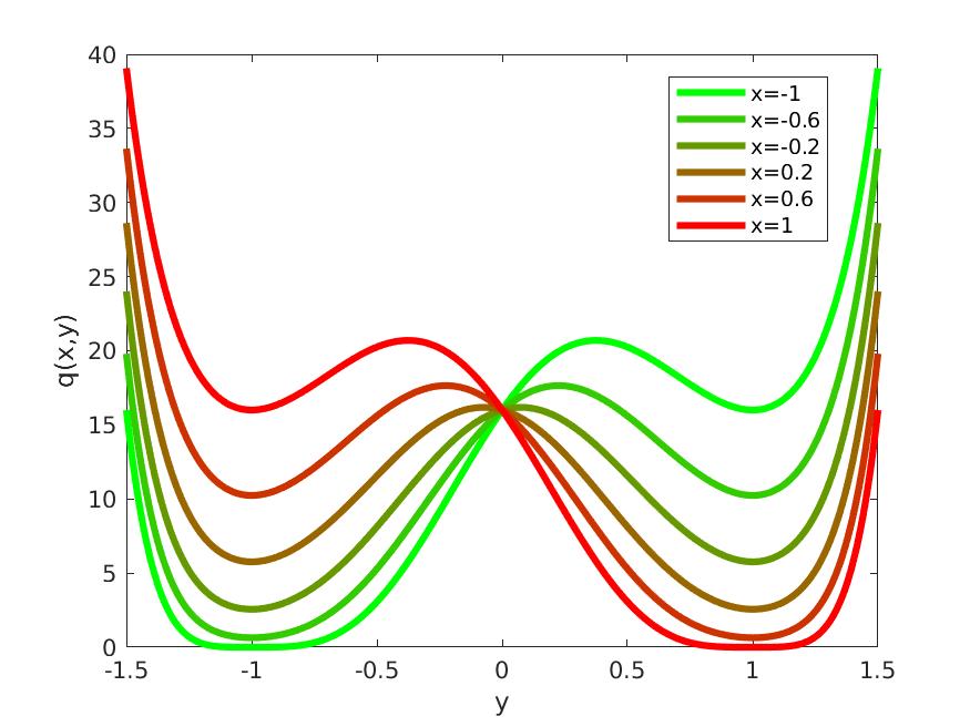
Consider the polynomial
| (2) |
One can easily check that
for any and . Note that since is positive for , it can be squared without changing the argmin in and hence we obtain a similar representation of the sign function in the form of partial minimization in of the degree 8 SOS polynomial , represented in Figure 1.
Example 2 (Absolute value as SOS partial minimum).
The reader may check that the argmin in of the (square of the positive) polynomial is equal to for all .
To the best of our knowledge, this work is the first contribution where this class of semi-algebraic functions is used for graph approximations. The present work shows how these functions may be used to approximate discontinuous functions accurately.
Comparison to existing approximation approaches:
A classical alternative to our approach would be to use -norm Legendre or Chebyshev approximations of the function which are also based on moment information. However these approaches only use moment information on the measure , i.e. is linear. Moreover, the support of this measure is not the graph of .
We claim that the full moment information provides useful additional data on the graph of which we can access using Christoffel-Darboux kernels associated with the measure in (1). Note that in interpolation applications, we have the possibility to estimate the higher order moments of from finitely many evaluations of through Riemann integral approximations or Monte-Carlo approximations for example. However, in situations where we have neither access to higher moments nor pointwise evaluation of , our method cannot be applied; signal processing applications are a typical case of the latter situations.
In general, approximating a discontinuous function is a challenge. Indeed, most well-known techniques suffer from the Gibbs phenomenon, i.e. the approximation produces oscillations at each point of discontinuity of , see e.g. [14] for a good survey on this topic. The main tools usually rely on properties of orthogonal polynomials [38] and the resulting approximations are based on a finite number of Fourier coefficients of the latter functions, i.e., typically first degree moment information on . Projecting a discontinuous function on a class of infinitely smooth functions is the typical mechanism producing Gibbs phenomenon. In order to get rid of such a curse, additional techniques and prior information is needed. A possible approach is reported in [11] in the univariate case ( in our notations), where a good approximation of locations of discontinuity points and jump magnitude is obtained by solving an appropriate (univariate) polynomial equation. Recent developments have effectively shown that such approaches may tame the Gibbs phenomenon [3, 4]. Iterative numerical methods can also be used to identify the points of discontinuities of (and of its derivatives) so as to construct accurate approximations locally in each identified interval, see e.g. [30] in the case of Chebyshev polynomials. However such ad-hoc techniques are very specific to the univariate setting.
On the contrary, our approach is not based on projection on a subspace of smooth functions, or identification of points of discontinuities of the function to be approximated. It is based on geometric approximation of the support of a singular measure using semi-algebraic techniques. An important feature of this approach is that the resulting approximant functions are not necessarily smooth, and furthermore, discontinuities (if any) can be treated implicitly only based on the whole moment information. As a result, we obtain a single approximation scheme, which (i) may adapt to the smoothness features of the target function without requiring prior knowledge of it, and (ii) can be used for multivariate , both points being important challenges regarding numerical approximation.
Description of our contribution
-
1.
We first provide a numerical scheme which allows to approximate the compact support of a measure which is singular with respect to the Lebesgue measure. We need to adapt the strategy of [25] which covered the absolutely continuous case. This result may be considered of independent interest and will be instrumental to providing convergence guarantees for our approach.
-
2.
Next, given a degree , we provide an approximation of the function and prove that the sequence converges pointwise to almost everywhere as well as in -norm as goes to infinity (under broad assumptions on ). Furthermore, if we assume more regularity on , then we also provide estimates for the rate of convergence. More precisely, we obtain for multivariate Lipschitz functions and for univariate functions of bounded variation.
-
3.
Finally, we provide some numerical examples to illustrate the efficiency of the method. We first use our algorithm to approximate discontinuous or non-smooth solutions of OCP or PDE problems based on the Moment-SOS hierarchy. These experiments empirically demonstrate the absence of Gibbs phenomena. We also provide an example where only samples of the measure under consideration are given and show that our algorithm also works well, even for moderate size samples, showing that moment input data could in principle be approximated using numerical integration methods.
Example 3 (Sign function).
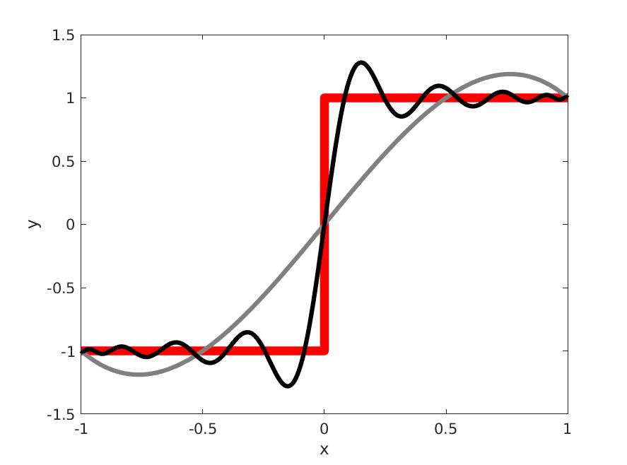
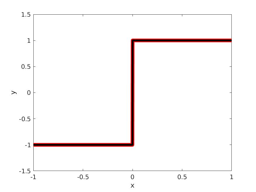
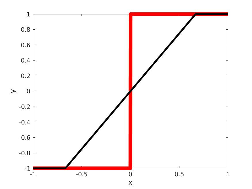
To give a flavor of what can be obtained numerically, consider the measure (1) supported on the graph of the function , with . In Figure 2 (right) the resulting approximation with a moment matrix of size and degree (i.e. moments) cannot be distinguished from . On the other hand, on the left, their Chebsyhev interpolants of degrees 4 and 20 (obtained with chebfun [9]) illustrate the typical Gibbs phenomenon, namely oscillations near the discontinuity points that cannot be attenuated by increasing the degree. This phenomenon can be reduced or suppressed by identifying the discontinuity points and splitting into intervals (as in e.g. [30] and also implemented in chebfun), but this strategy works only in the univariate case. In contrast, our algorithm does not attempt to approximate directly a univariate function with one or several univariate polynomials of increasing degree, but with the argmin of a bivariate polynomial of increasing degree. Moreover, our algorithm works also for multivariate functions, as shown by numerical examples later on.
1.3 Organization of the paper
Section 2 introduces the Christoffel-Darboux polynomial, its regularized version and our semi-algebraic approximant. In Section 3 the main results of the paper are collected, while their proofs are provided in Section 4. More precisely, we first give some quantitative estimates on the support of the measure and then prove the convergence of our approximant. Section 5 discusses computational issues and with the help of a simple Matlab prototype it illustrates the efficiency of our method on some examples. Finally, Section 6 collects some concluding remarks together with further research lines to be followed.
Notation
The Euclidean space of real-valued symmetric matrices of size is denoted by . Given a set in Euclidean space, its diameter is denoted by and its volume, or Lebesgue measure, is denoted by . For , the Lebesgue space consists of functions on whose -norms are bounded. Given a positive Borel measure , we denote by its support, defined as the smallest closed subset whose complement has measure zero.
Throughout the paper, denotes the dimension of the ambient space. Consistently with the notations introduced in Section 1 for stating Problem 1, we let . We denote by the algebra of multivariate polynomials of with real coefficients. For a given degree , the dimension of the vector space of polynomials of degree less than or equal to is denoted by .
2 Christoffel-Darboux approximation
This section describes our main approximant based on the Christoffel-Darboux kernel. We first introduce notations and definitions, describe our regularization scheme for the Christoffel-Darboux kernel and then describe our functional approximant based on moments.
2.1 Polynomials and moments
Following the notations introduced for stating Problem 1, any polynomial of degree can be expressed in the polynomial basis as with denoting its vector of coefficients. Recall that the moment matrix of degree of the measure reads
Since is positive semi-definite, it has a spectral decomposition
| (3) |
where is an orthonormal matrix whose columns are denoted , , and satisfy and if , and is a diagonal matrix whose diagonal entries are eigenvalues of the moment matrix. Each column is the vector of coefficients of a polynomial , , so that
| (4) |
2.2 Approximating the support from moments
Let us assume for now that the support of the measure has nonempty interior, then is positive definite for any , i.e., , . In this case, one can define the Christoffel-Darboux polynomial
| (5) |
It is known that sublevel sets of can be used to recover the support of for large , see for example [25] for an overview.
The goal of this work is to approximate the function . From a set theoretic perspective, this amounts to approximating the graph of whose closure is actually the support of the measure in (1). Hence the sublevel sets of are interesting candidates for this goal. However, in the case of the graph of a function, the construction given in (5) is not valid anymore since this graph is a singular set so that may not be positive definite and invertible. In this singular setting, one should ideally consider the following extended value Christoffel-Darboux polynomial:
| (6) |
where denotes the Moore-Penrose pseudo inverse. This is a natural extension of the Christoffel-Darboux polynomial to the singular case [32] and amounts to working in the Zariski closure of the graph of .
2.3 Regularization scheme
Spectral filtering:
Computing an object such as in (6) can be numerically sensitive since it essentially relies on pseudo-inverse which requires an eigenvalue thresholding scheme. This means that small perturbations of the moment matrix may lead to large changes of the output. Furthermore the candidate function takes finite values only on an algebraic set, and this situation is difficult to handle in finite precision arithmetic. One may rewrite the extended value polynomial (6) in the following form
where with for any and . One approach to restore stability is to use regularization techniques which replace the pseudo-inversion expressed through the function , by spectral filtering expressed through a different spectral function (see for example [7] for an illustration in the context of support estimation). Since the function is not regular, instead of studying the above defined extended value polynomial, one rather looks at the following polynomial
| (7) |
where is a parametrized family of spectral filtering regular functions satisfying, for any , . Common examples include
| Tikhonov regularization: | |||
| Spectral cut-off: | |||
| Ideal low-pass: |
We choose to work with the Tikhonov regularization as it has an intuitive measure space intepretation. We believe that our results can be generalized to different spectral filters.
Tikhonov regularization and measures:
Applying the Tikhonov spectral filter to (7) yields the following polynomial
| (8) |
where denotes the identity matrix of size . In order to use analytic tools, we need to provide an interpretation of the addition of diagonal elements in terms of measures. One therefore has to choose a polynomial basis for which the diagonal matrix is the moment matrix of a reference Borel measure on that we will denote . We make the following assumption which will be standing throughout the paper.
Assumption 1 (Reference measure and polynomial basis).
-
•
The reference measure is absolutely continuous with respect to the Lebesgue measure and it has compact support.
-
•
The polynomial basis is orthonormal with respect to the bilinear form induced by , that is if and otherwise.
The first part of Assumption 1 ensures that the moment matrix of is always positive definite. The second part of Assumption 1 provides the following relation:
| (9) |
An easy example of such a measure should be the following: considering a function whose domain of definition is contained in the unit cube of dimension and which takes values in , one might pick the uniform measure on the unit cube of dimension , for which moments are easy to compute.
Most importantly, using the notation in (5), this allows to express the polynomial of interest (8) as follows.
Definition 1 (Regularized Christoffel-Darboux polynomial).
The regularized Christoffel-Darboux polynomial is the SOS
| (10) |
This provides a geometric interpretation of the regularization parameter as a combination of two measures: which is supported on the graph of the function of interest and which is a reference measure, used for regularization purposes. The supported boundedness hypothesis in Assumption 1 will allow to provide quantitative estimates in further sections and it could in principle be replaced by a fast decreasing tail condition. An important example for measures satisfying Assumption 1 is the restriction of Lebesgue measure to the unit hypercube together with Legendre polynomials which form an orthonormal basis.
Making Assumption 1 is a slight restriction for which a few comments are in order. Firstly, this could be relaxed in various ways to remove the restriction on the polynomial basis, for example:
-
•
Replace the identity matrix by the moment matrix of ;
-
•
Add assumption on the spectrum of the moment matrix .
These would lead to a lot of technical complications and we find our results clearer and easier to state under Assumption 1. Secondly, working numerically with polynomials in the standard monomial basis is problematic in many situations. Better conditioned polynomial bases are often those enjoying orthonormality properties with respect to a certain reference measure, such as e.g. Chebyshev or Legendre polynomials. We would like to argue here that the restrictions induced by Assumption 1 are quite benign since it is already common in practice to work in such polynomial bases for numerical reasons.
2.4 Semi-algebraic approximant
Definition 2 (Semi-algebraic approximant).
The regularized Christoffel-Darboux semi-algebraic approximant is defined as follows:
| (11) |
Remark 1.
If and are semi-algebraic, then the set-valued map which associates to each the set
is semi-algebraic. Recall that a map is semi-algebraic if its graph is semi-algebraic. By the Tarski–Seidenberg Theorem (see for example [5, Theorem 2.6]), any first order formula involving semi-algebraic sets describes a semi-algebraic set. Since minima are described by first order formulas, the argmin of a polynomial on the compact semi-algebraic set is a compact semi-algebraic subset of , which is itself a subset of the real line. Hence the argmin set has a minimal element and the function in (11) is well defined.
Remark 2.
For clarity of exposition we describe our main results by considering that the partial minimization in over is exact. As will be seen from arguments in the proof, especially in the proof of Lemma 31, approximate minimization up to a factor of the order enjoys similar approximation properties. Indeed, in Remark 5, we mention the precision , where is chosen later on with more justifications in (14) to be of order .
The two parameters and control the behavior of the approximant . In latter sections, we describe an explicit dependency between and which allows to construct a sequence of regularization parameters , and we investigate the asymptotic properties of the sequence of approximants .
3 Main results
Our main theoretical contribution is an investigation of the relations between the function to be approximated and its regularized Christoffel-Darboux approximant under Assumption 1. In particular we are interested in building an explicit sequence and investigating the convergence for , fixed, as well as the convergence , when .
3.1 Convergence under continuity assumptions
The following section describes our main result regarding convergence of the approximant in (11) under different regularity assumptions for the function to be approximated. Let us define
Theorem 1.
Remark 3.
- •
-
•
Thanks to Egorov’s Theorem, pointwise convergence almost everywhere implies almost uniform convergence, that is uniform convergence up to a subset of whose measure can be taken arbitrarily small. Since we manipulate bounded functions, this in turn implies convergence in .
-
•
For Lipschitz continuous functions, we obtain an convergence rate in norm by setting .
-
•
The convergence rate for Lipschitz functions is slow and we observe in practice a much faster convergence. We conjecture that faster rates can be obtained for special classes of functions.
3.2 Convergence for univariate functions of bounded variation
Spaces of functions of bounded variations are of interest because many PDE problems are formulated on such spaces, see [1] for an introduction. Modern construction of such spaces is done by duality through measure theoretic arguments. Our main proof mechanisms rely on pointwise properties of the function , which are not completely captured by the measure theoretic construction.
We prove convergence for univariate bounded variation functions. The reason we are limited to the univariate setting is that we can use the classical definition of total variation which is directly connected to pointwise properties of the function of interest. We conjecture that the proposed approximation scheme is also convergent for multivariate functions of bounded variation, but we leave this question for future work.
Definition 3.
Let be a measurable function. The (Jordan) total variation norm of is given by
Theorem 2.
We remark that we obtain a convergence rate in . This result is a special case of a more general result described in Theorem 4 and proven later on.
3.3 Robustness to small perturbations
In many situations, one only has access to an approximation of the regularized Christoffel-Darboux polynomial. This is for example the case when applying the Moment-SOS hierarchy. At the end, one indeed obtains pseudo-moments of the measure under consideration, i.e. a vector of real numbers close to the actual moments of the measure. The moment matrix is then not as in (9) but a matrix close to it. The effect of this perturbation on the Christoffel-Darboux polynomial is captured by the following result.
Lemma 1.
Assume that the approximate moment matrix is positive definite and let
where we used the matrix operator norm. Then the polynomial satisfy
Proof: For any , we have
Remark 4 (Accuracy of the moments).
In this paper, we assume the existence of a positive number which makes the link between an approximated moment matrix and the real one, which exists in general, but estimates for are not known in general. Such an analysis has been performed for the moments themselves in [29], but not for moment matrices. Indeed, the bounds linking moment matrices and their corresponding depend nonlinearly on too many variables to obtain easily bounds on the approximated moment matrix and the real one. This is a topic of further investigation.
More generally, we can consider a robust Christoffel-Darboux function satisfying the following inequality.
Assumption 2.
For a given , let be a sequence of positive numbers and be a sequence of continuous functions over such that for any and any , we have
Note that Assumption 2 ensures that
| (12) |
Furthermore, one can always choose and which corresponds to the nominal case. The robust approximant is then defined similarly as in Definition 2.
Definition 4 (Robust semi-algebraic approximant).
Given a degree , a regularizing parameter , and a scalar , our robust approximant is defined as follows:
| (13) |
The main technical result of this paper is the following from which Theorem 1 directly follows.
Theorem 3.
Furthermore, we have the following robust convergence result for univariate functions of bounded variation, from which Theorem 2 directly follows.
Theorem 4.
The next section is dedicated to the proof of these theorems.
4 Proofs
This section is divided into several subsections. Subsection 4.1 gives some quantitative results on the estimation of the support of which does not depend on the nature of and could be of independent interest. More precisely, we show that the regularized Christoffel-Darboux polynomial takes large values outside the support of and smaller values inside. This is expressed by describing properties of certain sublevel sets of the polynomial being close to the support of . In subsection 4.2 we translate these geometric results in functional terms. In subsection 4.3, we prove our main results: the argument of the minimum of the regularized Christoffel-Darboux polynomial is close to the graph of the function .
4.1 Estimation of the support
In this section we build a polynomial sublevel set that will be instrumental for our proofs of convergence in functional terms. Note that in practice this sublevel set is not computed: we just focus on the argmin of the regularized Christoffel-Darboux polynomial. The contents of this section may be considered of independent interest.
For any and such that and for any , define
| (14) |
and
| (15) |
We aim at proving that the sublevel set is approaching the support of as goes to infinity, with a given convergence rate. It is precisely quantified with the following result which is illustrated in Figure 3.
Theorem 5.
For it holds
-
(i)
-
(ii)
For any ,
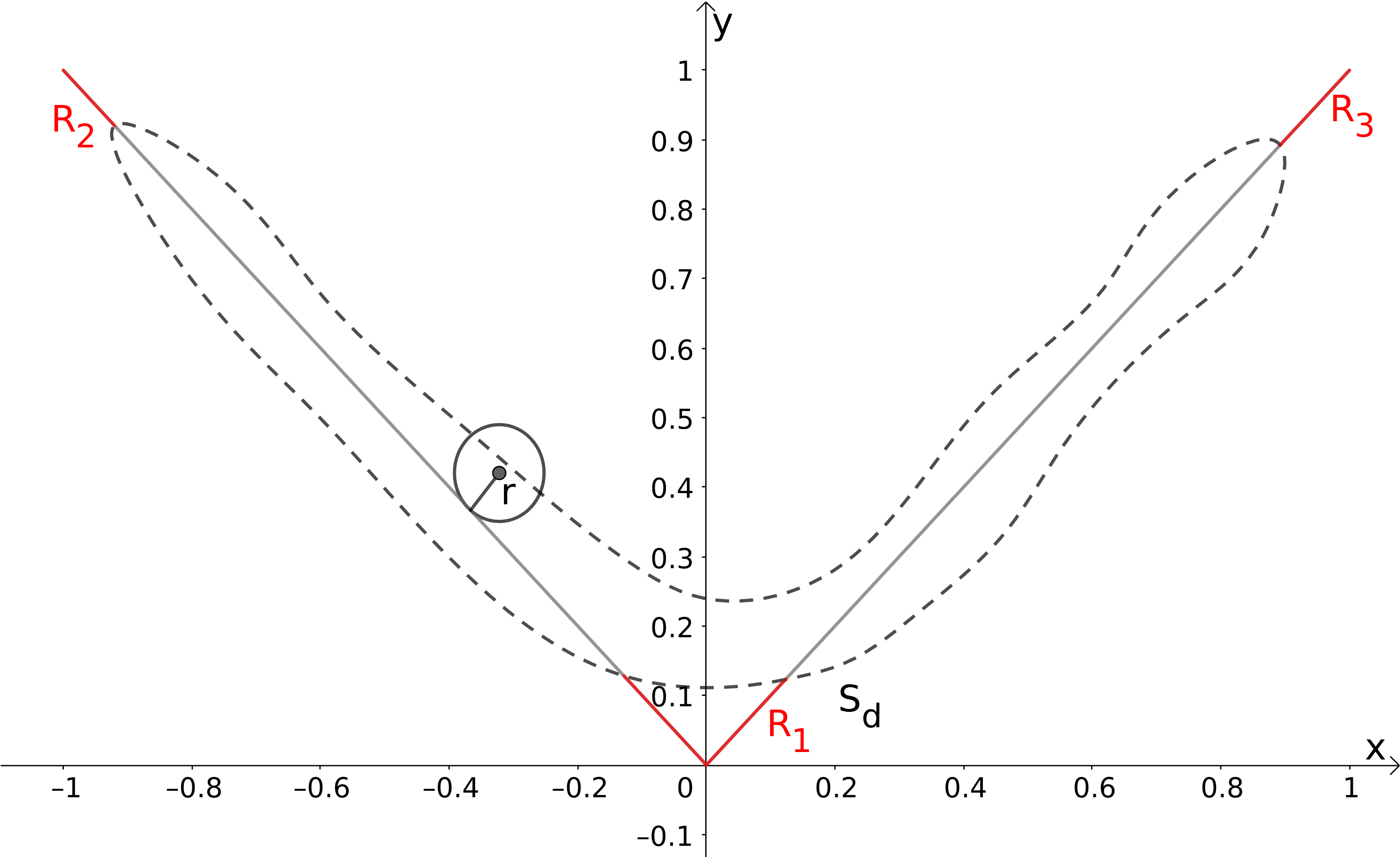
The results and techniques that we will use to prove this theorem are adapted from [25] which considers the absolutely continuous setting without regularization.
Proof of Theorem 5 (i) Using (10) and (4), we obtain
| (16) |
where the last inequality is given in [25, Lemma 6.5]. Using Markov’s inequality [36, Page 91] and (16) yields
| (17) |
Now using (12) and (15), we have the following implications
Hence . Using the expression of in (14) and the inequality (17), one has:
which concludes the proof of item of Theorem 5.
To carry out the proof of Theorem 5 (ii), we begin with a few lemmas. The following result is classical, see e.g. [25, Remark 3.6.] and [20, Equation (1.1.)].
Lemma 2.
Let , , , and be a polynomial of degree at most . Then
The following Lemma defines the needle polynomial, introduced first in [20], and gives a quantitative result crucial for our analysis.
Lemma 3 (Existence of a needle polynomial).
Let denote the euclidean ball of radius . Then, for all and , , there exists a polynomial of degree such that
| (18) |
A detailed proof is provided in [25, Lemma 6.3]. Thanks to the latter lemma, we can characterize the behavior of the regularized Christoffel-Darboux polynomial outside the support of :
Lemma 4.
Let , and . Recall that . Assume that . Then
| (19) |
Proof of Lemma 4: Let , , . Let and , arbitrary for the moment. Consider the affine map . Let be the degree polynomial given as in Lemma 3 such that
| (20) |
Let . The polynomial satisfies
| (21) |
Using Lemma 2 and the fact that we obtain
| (22) |
and
| (23) |
From (21), we deduce
| (24) |
| (25) |
Combining (22), (23) , (24) and (25), we obtain the following bounds
| (26) |
Recall that and were arbitrary. Now we can choose , in one of the identities in (26) (depending on the parity of ) to obtain
| (27) |
where the last inequality follows because the right hand side is strictly increasing as a function of and . This proves the desired result.
Let us give two additional simple technical lemmas.
Lemma 5.
For any ,
Proof of Lemma 5:
A simple analysis shows that the minimum is attained at . The lower bound follows because .
Lemma 6.
For any , we have
Proof of Lemma 6: Using the definition of in (14), we have
| (28) |
where the inequality follows from Lemma 5 with . This proves the desired result.
Proof of Theorem 5 (ii): We prove the result by contraposition. We have the following chain of implications for ,
| (29) |
where the first implication is from Lemma 4, the second implication is due to Lemma 6, the third implication is deduced from (12) and the last implication is from the definition of in (15).
4.2 Estimation of functions
We now translate Theorem 5 in functional terms. Considering that can be written as follows , let us introduce a specific set which will be of interest throughout the proof:
| (30) |
Lemma 7.
Suppose that . Then, we have
| (31) |
Proof of Lemma 31: For all and all measurable, one has
| (32) |
and hence
| (33) |
where . One can see from (30) that implies that and hence where denotes the complement of given in (15). We deduce that
| (34) |
and the result follows from Item (i) of Theorem 5.
Remark 5.
Thanks to Lemma 31, it is sufficient to prove the convergence of the approximated function in the set .
Proposition 1.
4.3 Proofs of the main theorems
We are now in position of proving Theorem 3. We start with the Lipschitz case, which is the simplest and conveys most of the ideas.
Proof of Theorem 3 (ii) Using Proposition 1: It remains to bound the term
| (36) |
For any define
| (37) |
with an arbitrary choice in the case where the argmin is not unique. Note that by continuity, the graph of is closed so that the minimum is attained. Using the definition of in (30), the fact that implies that
| (38) |
Moreover, Theorem 5 implies that
| (39) | ||||
where denotes the usual Euclidean distance in . Therefore, using Lipschitz continuity of , we have, for any ,
| (40) |
We deduce that
| (41) |
which concludes the proof.
We now turn to case (i), starting with the pointwise convergence.
Proof of Theorem 3 (i): We rely on a slighlty different use of Lemma 31. Choose and let
| (42) |
Lemma 31 ensures that so that
We have . This means that we have the two following properties, for almost every :
-
•
is continuous at (by assumption),
-
•
, , , (because .
Fix any such and for any consider
| (43) |
with an arbitrary choice when the argmin is not unique. Note that the support of is actually the closure of the graph of so that the minimum is attained. Using the definition of in (30), we have that for all which implies that
| (44) |
and Theorem 5 implies that
Since and is the closure of the graph of , there exists , such that
| (45) |
This concludes the proof of pointwise convergence since
and both terms tend to as , using (45) and continuity of at .
Convergence in follows from Egorov’s Theorem (see e.g. [33, chapter 18]): for any , there exists , measurable, of Lebesgue measure smaller than such that uniformly on . We have
By uniform convergence the second term goes to as , this shows that
Moreover, since was arbitrary, the limit is .
We now turn to the proof of convergence in norm for univariate functions of bounded variation.
Lemma 8.
Let be such that is finite and vanishes outside a segment . Let be positive constants. Let
Then
Proof of Lemma 8: This is a packing argument. Let and follow the recursive process, for , ,
This process must stop after a finite number of iterations. Indeed, the set consists of a finite union of intervals. At iteration , either one of these intervals is a subset of and then it is removed entirely from , or otherwise is contained in an interval which contains either or and the Lebesgue measure of is reduced by at least compared to , possibly creating a new interval.
Let be the last iteration, so that . By the iterative process, at each step, the measure of is reduced by at most and we have
so that
Finally, since the intervals , are disjoint, we have
which proves the desired result.
Proof of Theorem 4: For any consider
By Lemma 8, for any we have
| (46) |
Choose any and any such that and . Consider
| (47) |
with an arbitrary choice when the argmin is not unique.
Note that the support of is actually the closure of the graph of so that the minimum is attained. Using the definition of in (30), implies that
| (48) |
and Theorem 5 implies that
Since and is the closure of the graph of , there exists , such that
| (49) |
Now since and , we have . This entails
The latter expression does not depend on which was arbitrarily chosen outside of and . We deduce that
and the result follows by invoking Lemma 31 and using Inequality (46).
5 Numerical examples
5.1 Computational tractability
Working with a large class of approximation functions may pose computational difficulties. An advantage of our Christoffel-Darboux semi-algebraic approximant is that it can be computed efficiently.
If the input moments are exactly known and given in rational form, the Christoffel-Darboux polynomial to be partially minimized is obtained through formal inversion of the moment matrix. This operation has efficient implementations, namely polynomial time algorithms over rational entries, an example is given in [2].
In most of the applications, the moments are however known only approximately, and the Christoffel-Darboux polynomial is constructed via the numerical eigenvalue decomposition of the approximate moment matrix. Since the moment matrix is symmetric, its eigenvalue decomposition can be computed efficiently with numerically stable algorithms in floating point arithmetic [13].
In addition, the computational overhead of evaluating the semi-algebraic approximant at a given point is that of minimizing a univariate polynomial over the segment . The Lipschitz constant of a univariate polynomial with coefficients over is at most and hence grid search finds an -accurate solution to this problem using evaluations. In our case the entries of are polynomials in which are deduced from moment data so that for a fixed estimating and evaluating our semi-algebraic approximant up to a fixed arbitrary precision with rational inputs (moment matrix and ) can be done in polynomial time. Note also that our analysis shows that a level of precision of the order is sufficient so that the cost of the overall procedure has a complexity which is polynomial in the bit size of the moment matrix, the target evaluation point , as well as in , the degree bound.
5.2 Prototype code
We provide a simple Matlab prototype to validate our algorithm. All the examples described below are reproducible, and the Matlab scripts can be found at
homepages.laas.fr/henrion/software/momgraph
The calling syntax of the main routine is
[Y,P] = momgraph(M,X)
It takes as an input an approximate moment matrix
(in Matlab floating point format) for the monomial basis vector (in grevlex ordering), and a collection of points
(in Matlab floating point format) with . It outputs an approximation
(in Matlab floating point format) of the values , as well as a matrix of coefficients (in Matlab floating point format) of the vector of polynomials whose sum of squares yields the Christoffel-Darboux polynomial.
Our implementation is straightforward, not optimized for efficiency. The regularization parameter is set to the default value of , and the Christoffel-Darboux polynomial is computed from the eigenvalue decomposition (Matlab’s command eig) of the approximate moment matrix .
5.3 Sign function
Consider the measure supported on the graph of the sign function whose moments in the monomial basis on are
for . Here is an example of the use of momgraph to recover the sign function from the (floating point approximations) of the (exact) moments:
>> M % moment matrix of degree 4 for the sign function
M =
2.0000 0 0 0.6667 1.0000 2.0000
0 0.6667 1.0000 0 0 0
0 1.0000 2.0000 0 0 0
0.6667 0 0 0.4000 0.5000 0.6667
1.0000 0 0 0.5000 0.6667 1.0000
2.0000 0 0 0.6667 1.0000 2.0000
>> X = linspace(-1,1,1e3)’; % samples for evaluation
>> [Y,P] = momgraph(M,X); % Christoffel-Darboux approximation
>> plot(X,graph(X),’-r’,’linewidth’,6); hold on; % exact graph
>> plot(X,Y,’-k’,’linewidth’,3); xlabel(’x’); ylabel(’y’); % approximate graph
This code corresponds to a degree 4 approximation from a moment matrix of size 6 with 15 moments. A degree 2 approximation can be obtained from its 3 by 3 submatrix
>> M(1:3,1:3)
ans =
2.0000 0 0
0 0.6667 1.0000
0 1.0000 2.0000
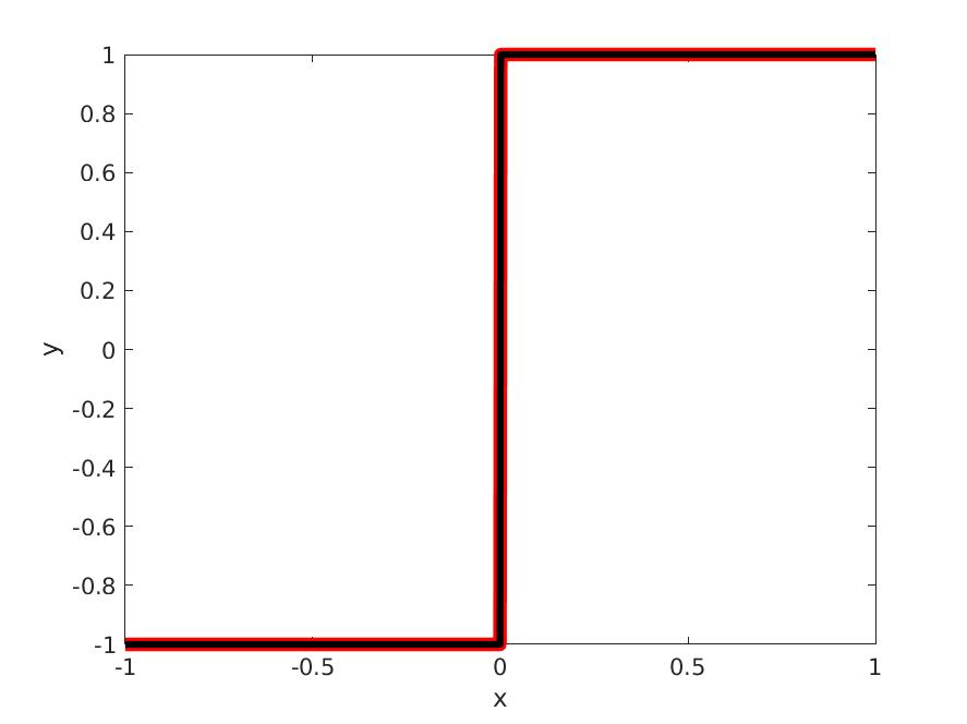
On Figure 4 we see that the resulting degree 4 semi-algebraic approximation cannot be distinguished from the graph of the sign function. Our semi-algebraic approximant is with the Christoffel-Darboux polynomial constructed as the sum of squares of the polynomials returned by the momgraph function:
>> mpol x y; b = mmon([x y],2); % GloptiPoly monomial vector of degree 2 >> P*b 6-by-1 polynomial vector (1,1):7071.0678-7071.0678y^2 (2,1):0.86713+9.4x^2-9.7305xy+0.86713y^2 (3,1):2.4315x-1.3013y (4,1):-0.53517+1.2757x^2+1.137xy-0.53517y^2 (5,1):0.29635x+0.55374y (6,1):0.29443+0.10761x^2+0.15643xy+0.29443y^2
We see in particular that the first polynomial is with a large scaling factor. This polynomial vanishes on the graphs of the functions and . The other polynomials are instrumental to determining which one of the two graphs corresponds to a given value of .
5.4 Discontinuous functions
Let us revisit the discontinuous univariate examples of [11]. Since in this case we do not have the analytic moments of the measure supported on the graph of the function to input to our algorithm, we use the empirical moment matrix computed by uniform sampling, i.e.
| (50) |
for sufficiently large, i.e. , and the monomial basis vector. Degree 10 semi-algebraic approximations are reported on Figure 5 for three benchmarks [11, Examples 65, 66, 67] of discontinuous functions , appropriately scaled in .
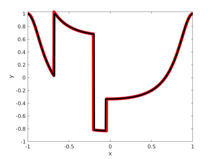
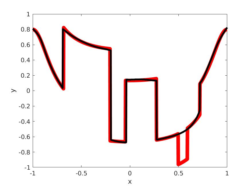
We observe that the second rightmost discontinuity in the middle example is not detected. Increasing the degree of the approximations does not fix the issue, and we believe that it is due to the poor resolution of the monomial basis. It would be more appropriate to use here a complex exponential basis (i.e. Fourier coefficients) or an orthogonal basis (e.g. Chebyshev or Legendre polynomials).
5.5 Interpolation


Suppose now that we have access only to the values of the function to be approximated at given sampling points , for small. Our algorithm takes as input the empirical moment matrix (50). On Figure 6, we revisit [11, Example 65] to study the effect of the number of samples on the quality of the approximation, for a uniform distribution of samples. We see that with 20 samples the function is already well approximated.
5.6 Recovering trajectories for optimal control
In [23], the moment-SOS hierarchy is applied to solve numerically non-linear optimal control of ODEs with polynomial data and semi-algebraic state and control constraints. Non-linear optimal control is formulated as a linear problem on moments of occupation measures supported on optimal trajectories. Let us show how numerical approximations of these moments obtained by semidefinite programming can be input to our algorithm to approximate optimal state and control trajectories.
Let us revisit the state-constrained double integrator problem of [23, Section 5.1] to approximate the time optimal trajectories. After a scaling of time, state and control, we use the Matlab interface GloptiPoly 3 and the conic solver MOSEK to compute the pseudo-moments of the occupation measure of degree up to 8. This can be achieved in less than 2 seconds on a standard desktop computer. From this output, we construct the 45-by-45 moment matrices of the control and state marginals, conditioned w.r.t. time. Using our notations, the independent variable is time, while the dependent variable is respectively the control, the first state and the second state. For this example, the analytic trajectories are available for comparison.
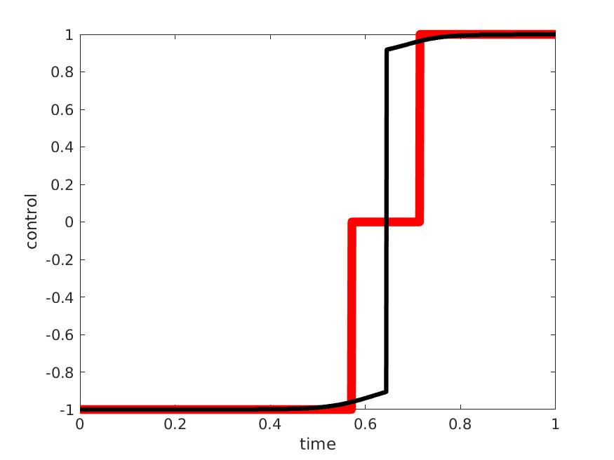

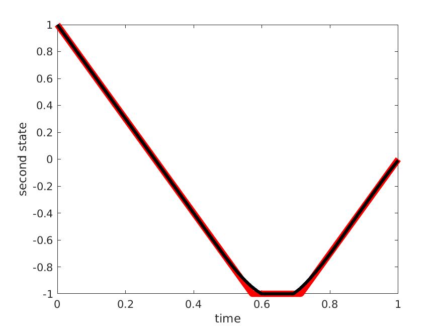
We see on Figure 7 that the state trajectory approximations are tight, whereas the control trajectory approximation misses partly the central region corresponding to the saturation of the second state. Indeed, since it is obtained by solving numerically the degree 8 semidefinite relaxation of the moment-SOS hierarchy, the approximated moment matrix differs from the exact moment matrix, and this has an impact on the quality of the Christoffel-Darboux approximation.

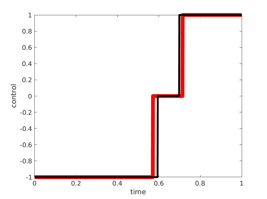
For this example, we can construct analytically the exact moment matrix of the control trajectory and observe that indeed its Christoffel-Darboux semi-algebraic approximation of degree 8 identifies well the optimal control trajectory switching times, see Figure 8.
5.7 Bivariate examples
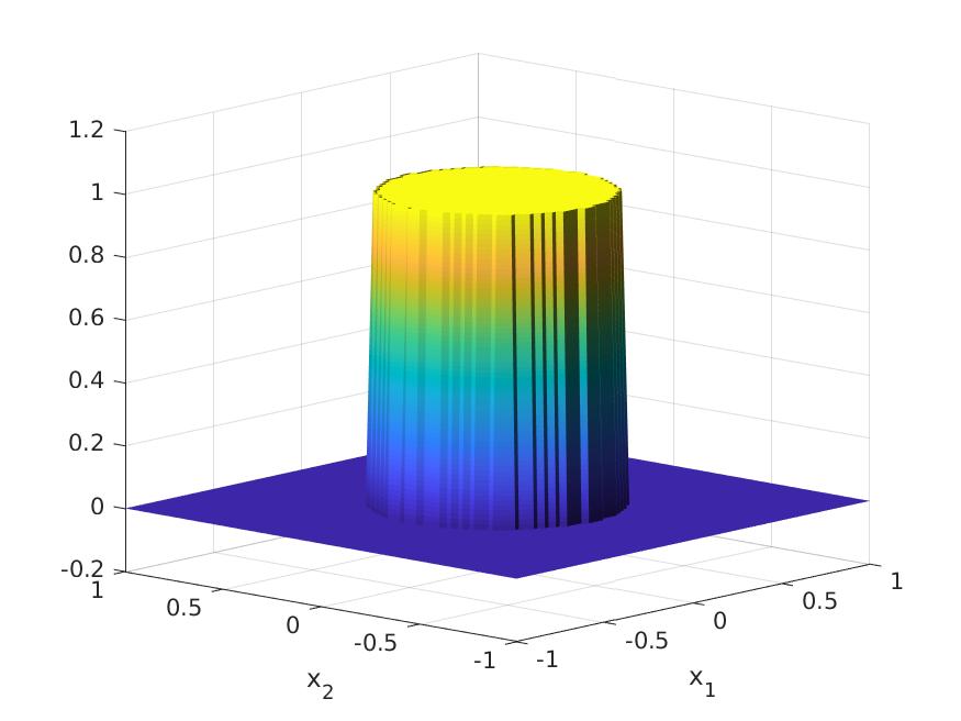
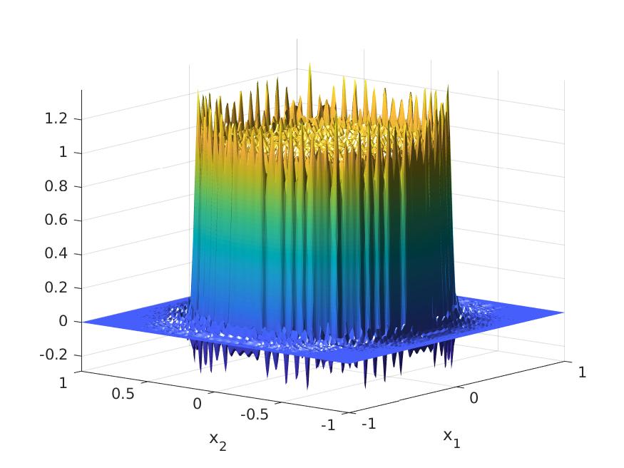
Consider the indicator function
of a centered disk of radius . We compute the emprical moments obtained by sampling points on a uniform grid of . With this input, our algorithm computes the degree 8 semi-algebraic approximation reported on Figure 9, to be compared with the Chebyshev polynomial approximation obtained from points by the chebfun2 command, showing the typical Gibbs phenomenon.
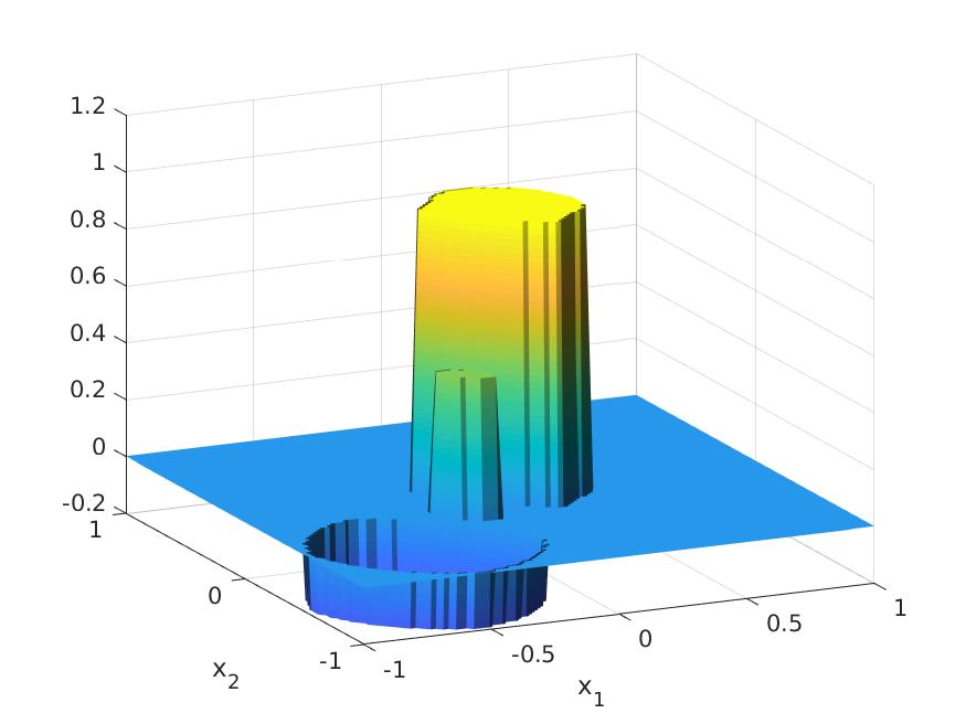
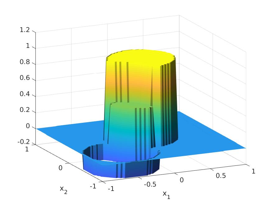
We perform the same computations for the piecewise constant function
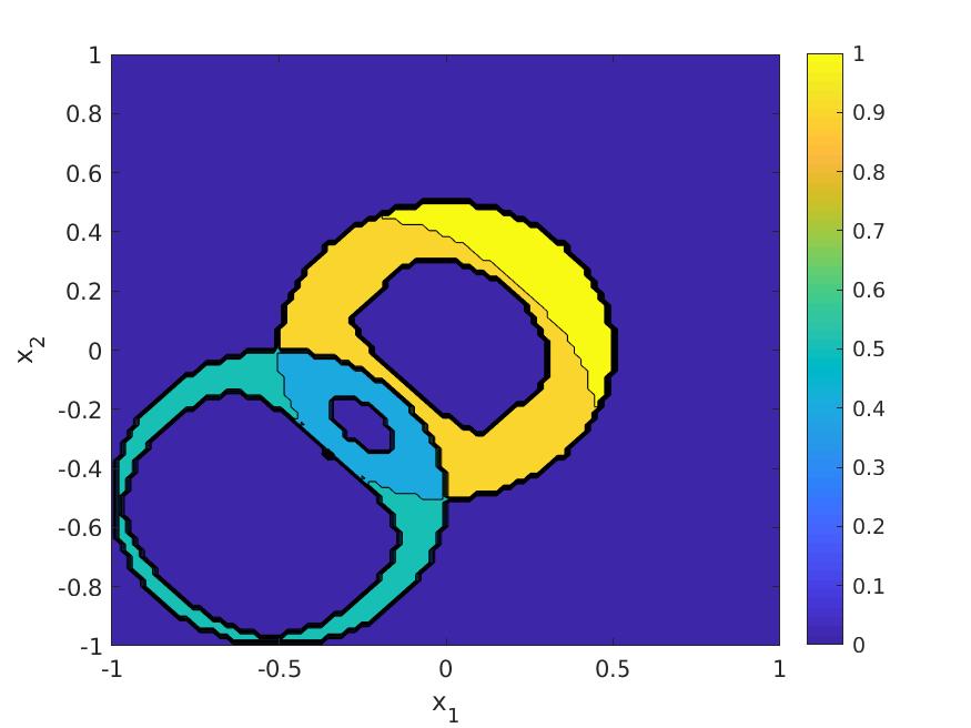
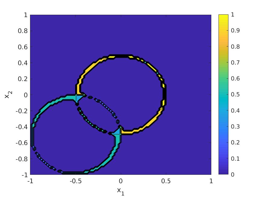
obtained as a superposition of signed indicator functions of two disks. Its degree 8 and 16 semi-algebraic approximations are reported on Figure 10. The absolute pointwise error between the approximations and the original function is displayed on Figure 11.
5.8 Discontinuous solutions of non-linear PDEs
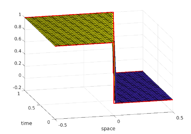

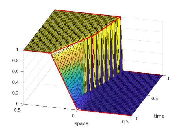
In [26], the moment-SOS hierarchy is applied to solve numerically a class of non-linear PDEs for which we known that classical (i.e. differentiable) solutions do not exist. The advantage of optimizing over occupation measures is that they can be supported on graphs of weak (i.e. possibly discontinuous) solutions. Let us show how approximate moments of these measures computed by semidefinite programming can be processed by our algorithm so as to recover these discontinuous solutions.
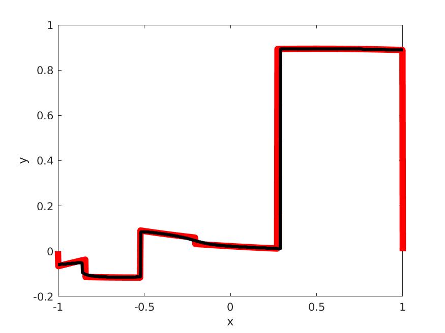
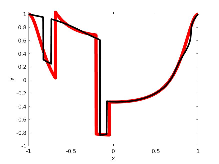
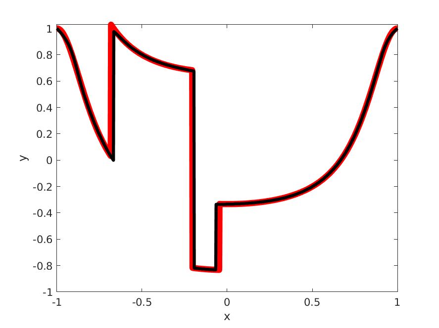
We focus on the Burgers equation and choose the initial data (a function of one space coordinate, at time zero) in a way that at a given time a shock appears, i.e. the solution becomes a discontinuous function of the space coordinate. Once the shock appeared, it propagates through, i.e. the discontinuity remains but its location varies. In Figures 12, 13, and 14 we show the graphs obtained from the moment relaxations proposed in [26]. In all cases we use the 969 triviate moments of degree 16 of the occupation measure (supported on time, space, and solution) to recover the graph of the approximated solution. For comparison we also sketch the analytic solution with red lines.
For the graphs in Figures 12 and 13, the approximated moments match the analytic moments up to an error of the order of . Our semi-algebraic approximations are almost identical to the analytic solution.
For the graph in Figure 14 the approximated moments are noticeably incorrect, i.e., the error is of order . Nevertheless, our semi-algebraic approximation is able to reproduce the graph of the solution quite accurately. In particular the propagation of the shock is retrieved from the moment data. However, the approximation is erroneous when the solution passes over from its continuous to its discontinuous part.
6 Conclusion
In this paper, we describe a new technique to estimate discontinuous functions from moment data, based on Christoffel-Darboux kernels. Instead of using polynomial or piecewise polynomial approximants, we use a class of semi-algebraic approximants, namely arguments of minima of polynomials. This is another occurrence of a lifting technique: instead of using only moments depending linearly on the function so as to recover directly the function, we use also moments depending non-linearly on the function so as to approximate the support of a measure concentrated on the graph of the function. We provide functional analytic and geometric convergence proofs. Finally, some numerical examples illustrate the efficiency of our algorithm.
We believe that this work opens the way to many other further research lines:
-
•
When applying the Moment-SOS hierarchy, the moments are numerical approximations of the real ones. It would be interesting to provide a sensibility analysis of the application of our algorithm for the real moments and the approximated ones. We believe that such an analysis can be performed, since promising results were achieved recently in [19] for the case of zero dimensional manifolds, i.e. unions of finitely many points.
-
•
It could also be interesting to investigate in a more quantitative way why the Gibbs phenomenon might be avoided or at least attenuated with the technique we provide. We believe that it is mainly due to the semi-algebraic point of view we are following.
-
•
We could also check whether our algorithm works as well when considering only the knowledge of Fourier coefficients, namely moments depending linearly on the function that we want to approximate. In many problems, this is the only measurement that we might have. This is therefore a partial moment information, and we may want to complement it with estimates of higher degree moments. This makes the problem challenging.
7 Acknowledgments
We are grateful to Quentin Vila for his technical input on discontinuous solutions of PDEs, and to Milan Korda, Victor Magron and Matteo Tacchi for interesting discussions. This work was partly funded by the ERC Advanced Grant Taming and was also conducted in the framework of the regional programme ”Atlanstic 2020, Research, Education and Innovation in Pays de la Loire, supported by the French Region Pays de la Loire and the European Regional Development Fund. E. Pauwels and J.B. Lasserre are also partially supported by the AI Interdisciplinary Institute ANITI funding through the french program “Investing for the Future PIA3”, under the Grant agreement number ANR-19-PI3A-0004.
References
- [1] L. Ambrosio, N. Fusco, D. Pallara. Functions of bounded variation and free discontinuity problems. Clarendon Press, Oxford, 2000.
- [2] E. H. Bareiss. Sylvester’s identity and multistep integer-preserving gaussian elimination. Math. Comput., 22(103):565–578, 1968.
- [3] D. Batenkov, Y. Yomdin. Algebraic Fourier reconstruction of piecewise smooth functions. Math. Comput., 81(277):277–318, 2012.
- [4] D. Batenkov. Complete algebraic reconstruction of piecewise-smooth functions from Fourier data. Math. Comput., 84(295):2329–2350, 2015.
- [5] M. Coste. An introduction to semialgebraic geometry. RAAG Network School, 145:30, 2002.
- [6] S. De Marchi, A. Sommariva, M. Vianello. Multivariate Christoffel functions and hyperinterpolation. Dolomites Research Notes on Approximation, 7, 2014.
- [7] E. De Vito, L. Rosasco, A. Toigo. Learning sets with separating kernels. Appl. Comput. Harmon. An., 37(2):185 – 217, 2014.
- [8] R. J. DiPerna. Measure-valued solutions to conservation laws. Arch. Ration. Mech. An., 88(3):223–270, 1985.
- [9] T. A. Driscoll, N. Hale, L. N. Trefethen (Editors). Chebfun Guide. Pafnuty Publications, Oxford, 2014.
- [10] C. F. Dunkl, Y. Xu. Orthogonal polynomials of several variables. Cambridge Univ. Press, 2014.
- [11] K. S. Eckhoff. Accurate and efficient reconstruction of discontinuous functions from truncated series expansions. Math. Comput., 61(204):745–763, 1993.
- [12] H. O. Fattorini. Infinite dimensional optimization and control theory, Cambridge Univ. Press, 1999.
- [13] G. H. Golub, C. F. Van Loan. Matrix Computations. 3rd Edition, The Johns Hopkins University Press, 1996.
- [14] D. Gottlieb, C.-W. Shu. On the Gibbs phenomenon and its resolution. SIAM Review, 39(4):644–668, 1997.
- [15] B. Gustafsson, M. Putinar, E.B. Saff, N. Stylianopoulos. Bergman polynomials on an archipelago: estimates, zeros and shape reconstruction. Adv. Math., 222(4):1405–1460, 2009.
- [16] K. Helmes, S. Röhl, R. H. Stockbridge. Computing moments of the exit time distribution for Markov processes by Linear Programming. Oper. Res., 49:516–530, 2001.
- [17] D. Hernández-Hernández, O. Hernández-Lerma, M. Taksar. The linear programming approach to deterministic optimal control problems. Applicationes Mathematicae, 24:17–33, 1996.
- [18] O. Hernández-Lerma, J. B. Lasserre. The Linear Programming Approach, pages 377–407 of Handbook of Markov Decision Processes, Springer, Boston, 2002.
- [19] I. Klep, J. Povh, J. Volčič. Minimizer extraction in polynomial optimization is robust. SIAM J. Optim., 28(4):3177-3207, 2018.
- [20] A. Kroó, D. S. Lubinsky. Christoffel functions and universality in the bulk for multivariate orthogonal polynomials. Can. J. Math., 65(3):600–620, 2012.
- [21] J. B. Lasserre. Moments, positive polynomials and their applications. World Scientific, 2010.
- [22] J.B. Lasserre. The Moment-SOS Hierarchy. Proceedings of the International Congress of Mathematicians (ICM), 4:3773–3794, 2018.
- [23] J. B. Lasserre, D. Henrion, C. Prieur, E. Trélat. Nonlinear optimal control via occupation measures and LMI relaxations. SIAM J. Control Optim., 47(4):1643–1666, 2008.
- [24] J. B. Lasserre, T. Prieto-Rumeau, M. Zervos. Pricing a class of exotic options via moments and SDP relaxations. Math. Finance, 16:469–494, 2006.
- [25] J.B. Lasserre, E. Pauwels. The empirical Christoffel function with applications in data analysis. Adv. Comp. Math. 45:1439–1468, 2019.
- [26] S. Marx, T. Weisser, D. Henrion, J. B. Lasserre. A moment approach for entropy solutions to nonlinear hyperbolic PDEs. Math. Control. Related Fields, 10:113–140, 2019.
- [27] A. Máté, P. G. Nevai. Bernstein’s inequality in for and bounds for orthogonal polynomials. Ann. Math., 111:145–154, 1980.
- [28] P. G. Nevai. Géza Freud, orthogonal polynomials and Christoffel functions. a case study. J. Approx. Theory, 48(1):3–167, 1986.
- [29] J. Nie and M. Schweighofer On the complexity of Putinar’s Positivstellensatz. Journal of Complexity, 23(1):135–150, 2007.
- [30] R. Pachón, R. B. Platte, L. N. Trefethen. Piecewise-smooth chebfuns. IMA J. Numer. Anal. 30(4):898–916, 2010.
- [31] J. B. Lasserre, E. Pauwels. Sorting out typicality with the inverse moment matrix sos polynomial. In Advances in Neural Information Processing Systems, pages 190–198, 2016.
- [32] E. Pauwels, M. Putinar, J.B. Lasserre. Data analysis from empirical moments and the Christoffel function. To appear in Found. Comp. Math., 2020.
- [33] H. Royden, P. Fitzpatrick. Real Analysis. 4th Edition, Pearson Education, 2010.
- [34] F. Santambrogio. Optimal Transport for Applied Mathematicians - Calculus of Variations, PDEs, and Modeling. Birkhäuser, 2015.
- [35] L. Silvestre Oscillation properties of scalar conservation laws Communications on Pure and Applied Mathematics 72(6):1321–1348, 2019
- [36] E. M. Stein, R. Shakarchi. Real analysis: measure theory, integration, and Hilbert spaces. Princeton Univ. Press, 2009.
- [37] R. H. Stockbridge. Discussion of dynamic programming and linear programming approaches to stochastic control and optimal stopping in continuous time. Metrika, 77(1):137–162, 2014.
- [38] G. Szegö. Orthogonal polynomials, Vol. 23. Amer. Math. Soc., 1939.
- [39] R. Vinter. Convex duality and nonlinear optimal control. SIAM J. Control. Optim., 31(2):518–538, 1993.