A Fundamental Plane for Gamma-Ray Pulsars

Abstract

We show that the $\gamma$-ray pulsar observables, i.e., their total $\gamma$-ray luminosity, $L_{\gamma}$, spectral cut-off energy, $\epsilon_{\rm cut}$, stellar surface magnetic field, $B_{\star}$, and spin-down power $\dot{\mathcal{E}}$, obey a relation of the form $L_{\gamma}=f(\epsilon_{\rm cut},B_{\star},\dot{\mathcal{E}})$, which represents a 3D plane in their 4D log-space. Fitting the data of 88 pulsars of the second Fermi pulsar catalog, we show this relation to be $L_{\gamma}\propto\epsilon_{\rm cut}^{1.18\pm 0.24}B_{\star}^{0.17\pm 0.05}\dot{\mathcal{E}}^{0.41\pm 0.08}$, a pulsar fundamental plane (FP). We show that the observed FP is remarkably close to the theoretical relation $L_{\gamma}\propto\epsilon_{\rm cut}^{4/3}B_{\star}^{1/6}\dot{\mathcal{E}}^{5/12}$ obtained assuming that the pulsar $\gamma$-ray emission is due to curvature radiation by particles accelerated at the pulsar equatorial current sheet just outside the light cylinder. Interestingly, the FP seems incompatible with emission by synchrotron radiation. The corresponding scatter about the FP is $\sim 0.35$dex and can only partly be explained by the observational errors while the rest is probably due to the variation of the inclination and observer angles. We predict also that $\epsilon_{\rm cut}\propto\dot{\mathcal{E}}^{7/16}$ toward low $\dot{\mathcal{E}}$ for both young and millisecond pulsars implying that the observed death-line of $\gamma$-ray pulsars is due to $\epsilon_{\rm cut}$ dropping below the Fermi-band. Our results provide a comprehensive interpretation of the observations of $\gamma$-ray pulsars, setting requirement for successful theoretical modeling.

1. Introduction

Since its launch in 2008, the Fermi Gamma-Ray Space Telescope, has increased by many-fold the number of $\gamma$-ray pulsars. More specifically, Fermi has detected over 230 new $\gamma$-ray pulsars to date (117 of which are included in the Second Fermi Pulsar Catalog (2PC), Abdo et al., 2013). The large number of newly discovered $\gamma$-ray pulsars show a number of trends and correlations among their observed properties, which probe the underlying physics connected to their emission.

On the theoretical side, there has been tremendous progress in modeling global pulsar magnetospheres. The Force-Free (FF) solutions (Contopoulos et al., 1999; Timokhin, 2006; Spitkovsky, 2006; Kalapotharakos & Contopoulos, 2009) despite their ideal (i.e., dissipationless) character revealed that the equatorial-current-sheet (ECS), which emerges at and beyond the light-cylinder (LC) is a good candidate for the observed $\gamma$-ray pulsar emission (Contopoulos & Kalapotharakos, 2010; Bai & Spitkovsky, 2010).

Later studies of dissipative macroscopic solutions (Kalapotharakos et al., 2012; Li et al., 2012) confirmed, that near FF-conditions, the ECS is indeed the main dissipative region with high accelerating electric-field components, $E_{\rm acc}$. More recently, the approach of kinetic particle-in-cell (PIC) simulations (Philippov & Spitkovsky 2014; Chen & Beloborodov 2014; Cerutti et al. 2016[C16]; Philippov & Spitkovsky 2018[PS18]; Kalapotharakos et al. 2018[K18]; Brambilla et al. 2018) confirmed the general picture that $\gamma$-ray pulsars possess a field structure resembling the FF one while the high-energy emission takes place near the ECS outside the LC. The advantage of the latter approach is that it provides particle distributions that are consistent with the corresponding field structures.

Kalapotharakos et al. (2014), Brambilla et al. (2015), and Kalapotharakos et al. (2017) assuming curvature radiation (CR) emission from test particles in dissipative macroscopic solutions were able to reproduce the radio-lag $\delta$ vs. peak-separation $\Delta$ correlation of the $\gamma$-ray profiles depicted in 2PC while a comparison between the model and the observed cutoff energies, $\epsilon_{\rm cut}$, revealed a relation between the plasma conductivity of the broader ECS region as a function of the spin-down power, $\dot{\mathcal{E}}$.

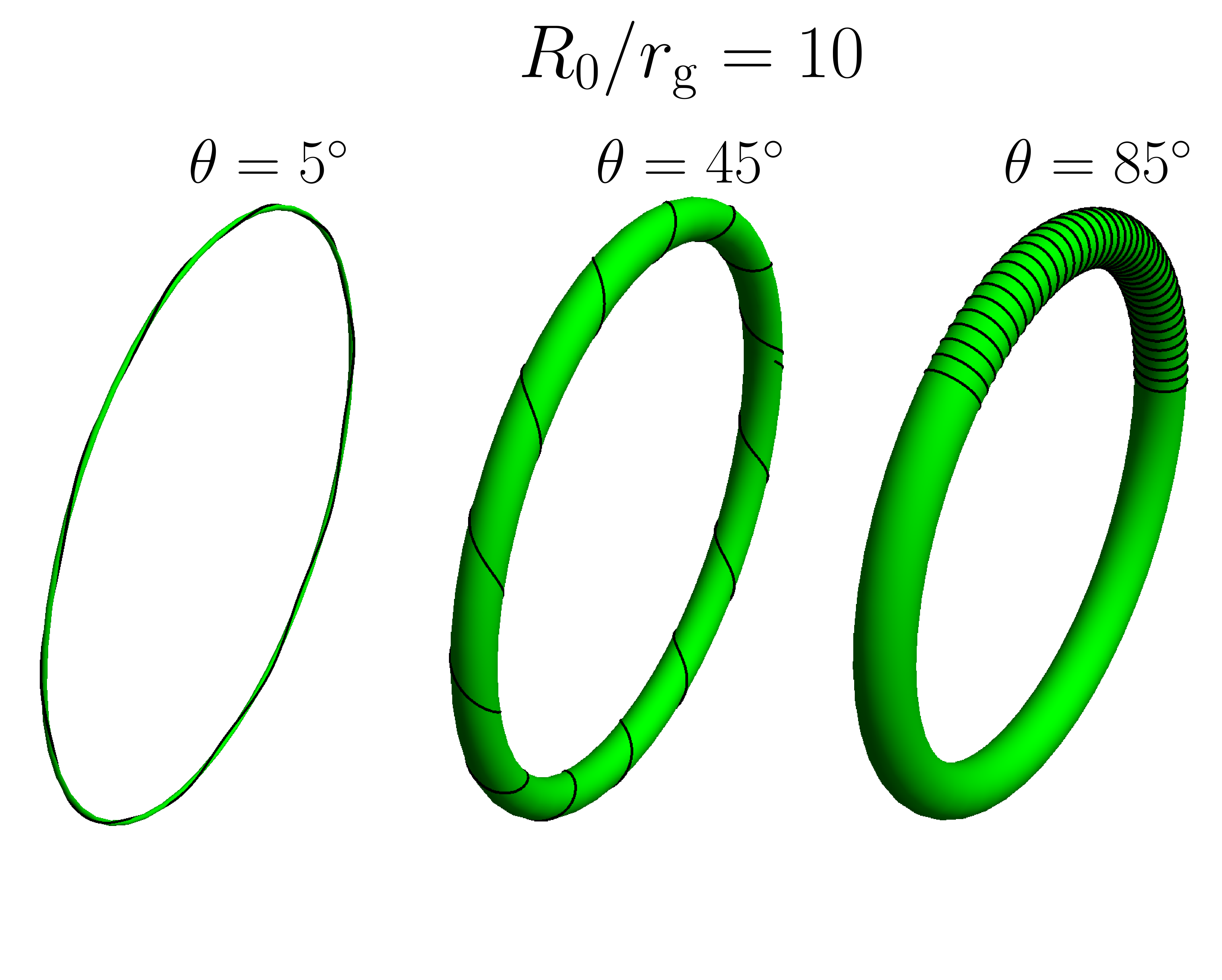
Figure 1.— The particle orbit for the indicated pitch-angle, $\theta$-values. The corresponding motion takes place on a torus with radii $R_{0}$ and $r_{\rm g}\sin\theta$. For $\theta\to 0^{\circ}$, $R_{\rm C}\to R_{0}$ while for $\theta\to 90^{\circ}$, $R_{\rm C}\to r_{\rm g}$.

The PIC simulations of K18, taking into account the contribution of CR (by appropriately rescaling the particle energies to realistic values), revealed a relation between the particle injection rate and $\dot{\mathcal{E}}$ that reproduces the observed range of $\epsilon_{\rm cut}$-values (i.e., $1-6\leavevmode\nobreak\ \rm{GeV}$).

C16 and PS18 presented PIC simulations of single particle injection rates and claimed that the corresponding high-energy emission is due to synchrotron radiation (SR).

Thus, even though there is consensus that the main component of the observed pulsar $\gamma$-ray emission originates from regions near the ECS there still is an open question about which radiative process dominates in the Fermi band. Moreover, the recent detections by MAGIC and HESSII of very high energy (VHE) emission from the Crab (Ansoldi et al., 2016), Vela (Djannati-Ataï et al., 2017), and Geminga (Lopez et al., 2018) pulsars imply an additional emission component, and inverse Compton (IC) seems to be the most reasonable candidate (Rudak & Dyks, 2017; Harding et al., 2018). In any case, the multi-TeV photon energies detected imply very high particle energies ($\gamma_{\rm L}>10^{7}$), which favors CR over SR.

In this letter, we explore the effectiveness of CR and SR to explain the Fermi spectra, mainly under the assumption that the acceleration and radiative energy loss occurs in the same location. This is a different SR-regime from that in C16 and PS18, who assume that acceleration and radiation, due to reconnection in the ECS, are spatially uncoupled. Our results show that the observables of all the Fermi pulsars, i.e., young (YP) and millisecond (MP), are consistent with CR emission. More specifically, our analysis shows that the Fermi YPs and MPs lie on a 3D fundamental plane (FP) embedded in the 4D space of the total $\gamma$-ray luminosity, $L_{\gamma}$, $\epsilon_{\rm cut}$, the stellar surface magnetic-field, $B_{\star}$, and $\dot{\mathcal{E}}$. This FP is in full agreement with the theoretical predictions of CR-regime emission.

2. Reverse Engineering

The $\epsilon_{\rm cut}$-values observed by Fermi provide an excellent model diagnostic tool. Their variation is small while their value determination is robust. We note, however, that the $\epsilon_{\rm cut}$-values depend on the adopted spectral fitting model, which in the 2PC reads $dN/d\epsilon\propto\epsilon^{-\Gamma}\exp(-\epsilon/\epsilon_{\rm cut})$, where $\Gamma$ is the spectral index. Nonetheless, the apex energies, $\epsilon_{\rm A}$ of the spectral energy distributions are not much different than the $\epsilon_{\rm cut}$-values corresponding to the model adopted in 2PC. Actually, $\epsilon_{\rm A}=(2-\Gamma)\epsilon_{\rm cut}$ and therefore, only for $\Gamma\approx 2$, $\epsilon_{\rm A}$ deviates considerably from $\epsilon_{\rm cut}$. A detailed discussion about the best fitting function-model goes beyond the scope of this study. For the rest of the letter, we assume the $\epsilon_{\rm cut}$-values presented in the 2PC, which we believe accurately reflect the characteristic emission energies.

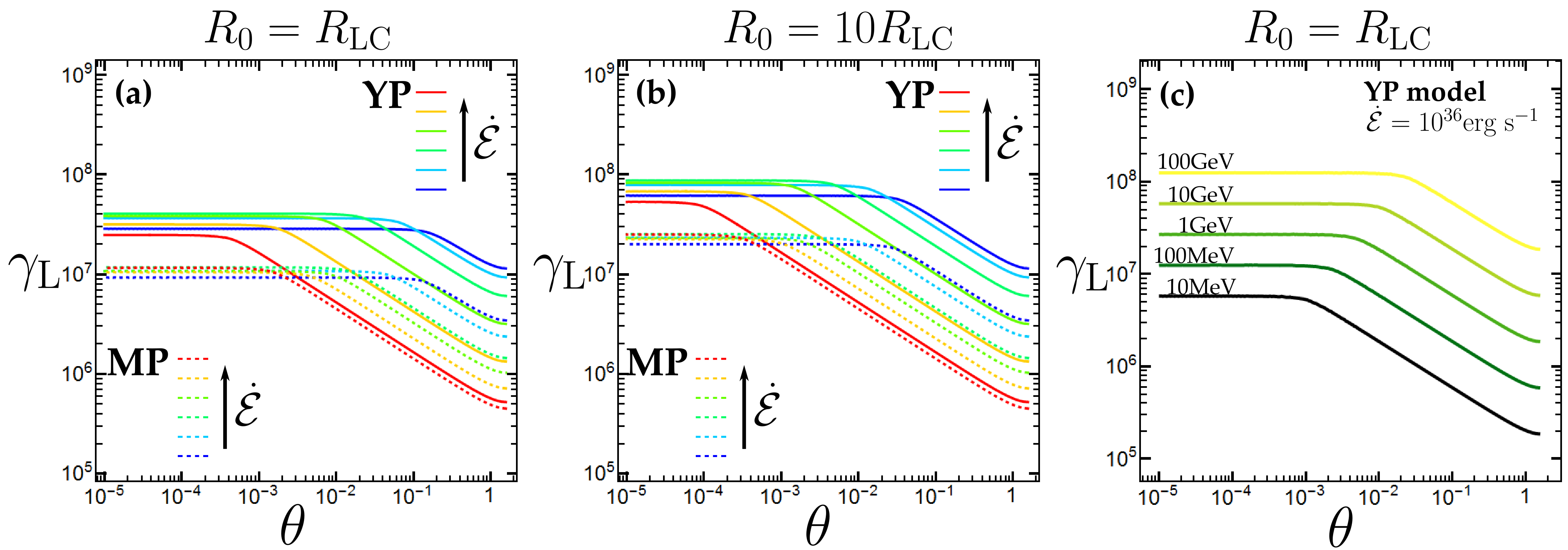
Figure 2.— (a) The $\gamma_{\rm L}$ vs. $\theta$ relations that reproduce the $\epsilon_{\rm cut}$-values corresponding to the different $\dot{\mathcal{E}}$-values (different colors) for YPs (solid lines) and MPs (dashed lines). These relations assume motion at the LC and $R_{0}=R_{\rm LC}$. (b) Similar to (a) but for $R_{0}=10R_{\rm LC}$. (c) The $\gamma_{\rm L}$ vs. $\theta$ relations for the YP model with $\dot{\mathcal{E}}=10^{36}{\rm erg\;s^{-1}}$ that reproduce the indicated $\epsilon_{\rm cut}$-values.

We consider a charged particle that is moving in an arbitrary electromagnetic field. In Appendix A, we show that the trajectory radius of curvature, $R_{\rm C}$, depends mainly on the maximum field value ($\max(E,B)$) and the generalized pitch-angle, $\theta$ that measures the deviation of particle velocity from the locally defined asymptotic trajectory. Below, we assume a magnetically-dominated field structure where the local $R_{\rm C}$ of the asymptotic flow, which in this case is the guiding-center trajectory, is $R_{\rm 0}$. The position vector $\mathbf{r}=(x,y,z)$ of a relativistic particle, without loss of generality, can be locally described by

$$\begin{split}x&=r_{\rm g}\sin\theta\;\sin\omega_{\rm g}t\\ y&=(R_{\rm 0}+r_{\rm g}\sin\theta\;\cos\omega_{\rm g}t)\cos\left(\frac{c}{R_{\rm 0}}\cos\theta\;t\right)\\ z&=(R_{\rm 0}+r_{\rm g}\sin\theta\;\cos\omega_{\rm g}t)\sin\left(\frac{c}{R_{\rm 0}}\cos\theta\;t\right)\end{split}$$ (1)

with $r_{\rm g}$ the gyro-radius, $\omega_{\rm g}=c/r_{\rm g}$, the gyro-frequency, and $t$ the time. The motion corresponding to Eqs.(1) takes place on a 2D torus with radii $R_{\rm 0}$ and $r_{\rm g}\sin\theta$. Thus, the orbital $R_{\rm C}$ is a function of $\theta$. As $\theta$ goes from 0 to $\pi/2$, $R_{\rm C}$ goes from $R_{\rm 0}$ to $r_{\rm g}$, respectively (see Fig.1). We note that particle trajectories corresponding to different field configurations have similar $(R_{\rm C},\theta)$-relations taking always into account that the generalized $r_{\rm g}$ is determined by the corresponding maximum field-value (Appendix A). The $\epsilon_{\rm cut}$-value of the corresponding spectrum reads

$$\epsilon_{\rm cut}=\frac{3}{2}c\hbar\frac{\gamma_{\rm L}^{3}}{R_{C}(\theta)}$$ (2)

where $\hbar$ is the reduced Planck constant.

Assuming motion near the LC, we set $R_{\rm 0}=R_{\rm LC}$ and $B=B_{\rm LC}$. In Fig.2a, we plot $\gamma_{\rm L}$ vs. $\theta$, for different $\dot{\mathcal{E}}$-values of YPs and MPs that reproduce the $\epsilon_{\rm cut}$ corresponding to the empirical $\epsilon_{\rm cut}-\dot{\mathcal{E}}$ relations

$$\begin{split}\epsilon_{\rm cutYP}&=10^{-103.5+5.75\log\dot{\mathcal{E}}-0.0795\log^{2}\dot{\mathcal{E}}}\\ \epsilon_{\rm cutMP}&=10^{-12.47+0.5708\log\dot{\mathcal{E}}-0.00571\log^{2}\dot{\mathcal{E}}}\\ (\epsilon_{\rm cutYP}&,\;\epsilon_{\rm cutMP}\;\text{in GeV and }\dot{\mathcal{E}}\text{ in }\rm{erg\;s^{-1}})\end{split}$$ (3)

presented in Kalapotharakos et al. (2017). Each line corresponds to different combinations of stellar surface magnetic-field, $B_{\star}$ and period, $P$ (i.e., different $\dot{\mathcal{E}}$) for YPs (solid lines) and MPs (dashed lines). The adopted cases (i.e., $B_{\star},P$ values) are the same as those presented in Table 2 of K18. More specifically, the $\dot{\mathcal{E}}$-values corresponding to the 6 YP curves are

$$\sim(10^{33},\leavevmode\nobreak\ 10^{34},\leavevmode\nobreak\ 10^{35},\leavevmode\nobreak\ 10^{36},\leavevmode\nobreak\ 10^{37},\leavevmode\nobreak\ 10^{38})\;\rm erg\;s^{-1}$$

while those corresponding to the 6 MP curves are

$$\sim(10^{32},\leavevmode\nobreak\ 10^{33},\leavevmode\nobreak\ 10^{34},\leavevmode\nobreak\ 4\times 10^{34},\leavevmode\nobreak\ 10^{35},\leavevmode\nobreak\ 10^{36})\;\rm erg\;s^{-1}.$$

For each case, a particle should either lie on a point of these lines or move along these lines in order to emit at the corresponding $\epsilon_{\rm cut}$-value. The $\gamma_{\rm L}$-value for $\theta\rightarrow 0$ (i.e., CR-regime) does not vary significantly with $\dot{\mathcal{E}}$ but is always higher than the value corresponding to $\theta\rightarrow\pi/2$ (i.e., SR-regime). Moreover, the ratio between the $\gamma_{\rm L}$-values corresponding to the two regimes increases with $\dot{\mathcal{E}}$.

In Fig.2b, we show the $\gamma_{\rm L}-\theta$ relations corresponding to $R_{\rm 0}=10R_{\rm LC}$. The $\gamma_{\rm L}$-ratio between the CR and SR regimes increase by a factor of $\sqrt[3]{10}$. In Fig.2c, we plot the $\gamma_{\rm L}-\theta$ relations for the fourth case of YPs (i.e., $\dot{\mathcal{E}}\approx 10^{36}\rm erg\;s^{-1}$) that produce the indicated $\epsilon_{\rm cut}$-values. We see that small deviations of $\gamma_{\rm L}$ and $\theta$ can significantly change the spectrum $\epsilon_{\rm cut}$-value.

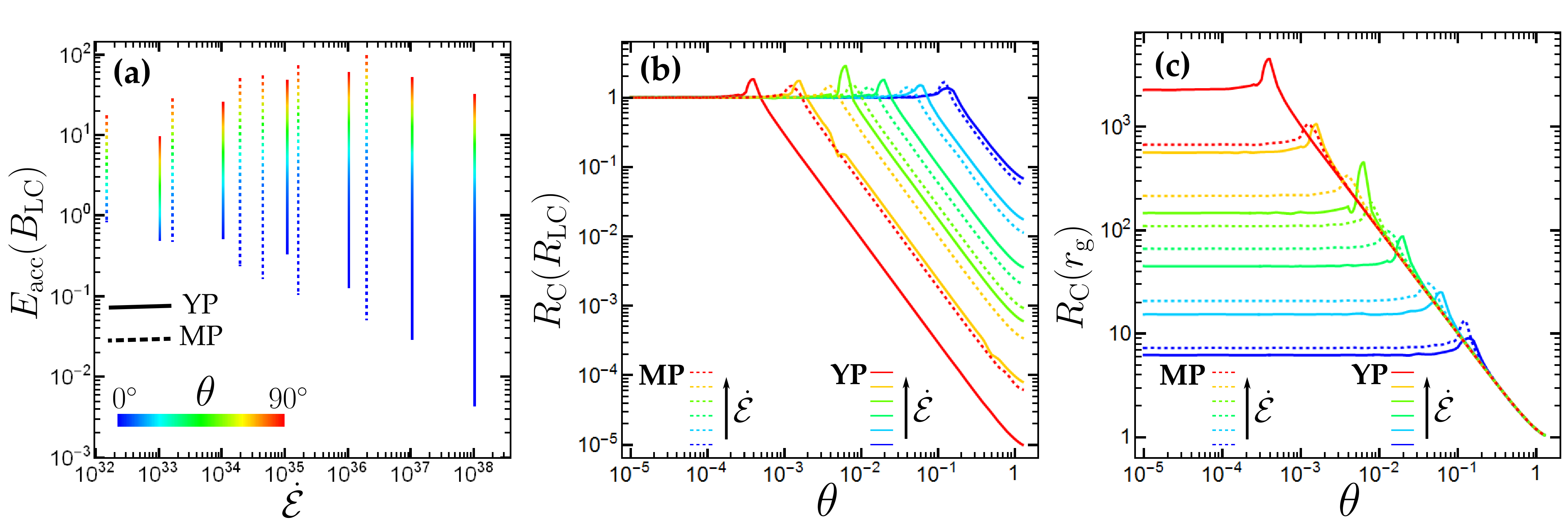
Figure 3.— (a) The $E_{\rm acc}$ in the corresponding $B_{\rm LC}$ units as a function of $\dot{\mathcal{E}}$ for MPs (dashed lines) and YPs (solid lines). The colors along the lines denote the $\theta$-value according to the indicated color-bar. (b) The $R_{\rm C}$ in $R_{\rm LC}$ units as a function of $\theta$ for the different YP and MP models. (c) Similar to (b) but the $R_{\rm C}$ is measured in $r_{\rm g}$ units. For all the cases, $R_{0}=R_{\rm LC}$ is assumed.

In order for particles to continue emitting at the desired $\epsilon_{\rm cut}$, the $\gamma_{\rm L}-\theta$ constraint should be sustained. In regions of high acceleration, $\theta$ normally decreases not only because of the relative rapid decrease of the perpendicular momentum component, which is the result of the radiation-reaction but also because of the increase of the parallel momentum component, which is the result of acceleration. The corresponding $\gamma_{\rm L}$ may increase or decrease depending on the balance between the radiation-reaction and the accelerating forces. These variations make the particles divert from the corresponding $\gamma_{\rm L}-\theta$ line. Balancing the radiation losses with the energy gain due to the accelerating fields,

$$\frac{2q_{\rm e}^{2}\gamma_{\rm L}^{4}}{3m_{\rm e}cR_{\rm C}(\theta)^{2}}=\frac{q_{\rm e}\mathbf{v}\cdot\mathbf{E}}{m_{\rm e}c^{2}}$$ (4)

can preserve $\gamma_{\rm L}$ but not $\theta$. This does not affect the CR-regime, but for the decreasing segment of the lines (Fig.2) the corresponding rapid decrease of $\theta$ (i.e., increase of $R_{\rm C}$) tends to destroy the balance and therefore the $\epsilon_{\rm cut}$. Thus, the $\theta$-value should be sustained by another mechanism (e.g. a heating process). In such a case, the development of noisy/fluctuating electric components in the perpendicular direction could in principle sustain $\theta$.

Taking into account the above assumptions, we can calculate the $E_{\rm acc}$ corresponding to each $\theta$-value (assuming preserved $\gamma_{\rm L},\leavevmode\nobreak\ \theta$ values). In Fig.3a, we plot the $E_{\rm acc}$ (in $B_{\rm LC}$ units) for the different YP and MP models (i.e., different $\dot{\mathcal{E}}$) and for the different $\theta$-values. For small $\theta$ (i.e., CR-regime), $E_{\rm acc}$ decreases with $\dot{\mathcal{E}}$ and it saturates for smaller $\dot{\mathcal{E}}$ to a value $\approx B_{\rm LC}$. For higher $\theta$, the $E_{\rm acc}$ increases considerably to a value even above $B_{\rm LC}$. In this case, the problem is that the required $E_{\rm acc}$-value is well above its upper limit, which is determined by the surrounding $B$-field (i.e., $B_{\rm LC}$). Nonetheless, for $R_{0}>R_{\rm LC}$ the lower envelope of Fig. 3a moves towards lower values allowing larger parts of $\theta>0$ with $E_{\rm acc}<B_{\rm LC}$.

In Figs.3b,c, we plot the $R_{\rm C}$ as a function of $\theta$ in units of the corresponding $R_{\rm LC}$ and $r_{\rm g}$, respectively. We see that $R_{\rm C}$ becomes a certain fraction of $R_{\rm LC}$ ($r_{\rm g}$), for all $\dot{\mathcal{E}}$-values, for $\theta\lesssim 10^{-3}$ ($\theta\gtrsim 10^{-1}$). Thus, in the pure CR-regime $R_{\rm C}\propto R_{\rm LC}$ while in the pure SR-regime $R_{\rm C}\propto r_{\rm g}$.

3. The Fundamental Plane of Gamma-Ray Pulsars

In Appendix B, we present, for both the CR and SR processes, relations between $L_{\gamma},\leavevmode\nobreak\ \epsilon_{\rm cut},\leavevmode\nobreak\ B_{\star}$, and $\dot{\mathcal{E}}$, always assuming emission at the LC near the ECS. These relations imply the existence of a 3D or 2D (depending on the regime) FP embedded in the 4D or 3D variable-space.

The Fermi-data allows the investigation of the actual behavior of the $\gamma$-ray pulsar population. We consider the function model $L_{\gamma}=A\;\epsilon_{\rm cut}^{a}\;B_{\star}^{b}\;\dot{\mathcal{E}}^{d}$ and we calculate the best-fit parameter-values taking into account the 88 2PC YPs and MPs with published $L_{\gamma}$ and $\epsilon_{\rm cut}$ values. Applying the least-squares method in $\log$-space, considering the same weight for every point, we get the best-fit relation

$$L_{\gamma(3D)}=10^{14.2\pm 2.3}\;\epsilon_{\rm cut}^{1.18\pm 0.24}\;B_{\star}^{0.17\pm 0.05}\;\dot{\mathcal{E}}^{0.41\pm 0.08}$$ (5)

where $\epsilon_{\rm cut}$ is measured in MeV, $B_{\star}$ in G, and $L_{\gamma},\leavevmode\nobreak\ \dot{\mathcal{E}}$ in $\rm erg\;s^{-1}$. We note that the $B_{\star}$-values have been derived assuming the FF $\dot{\mathcal{E}}$-relation for the inclination-angle, $\alpha=45^{\circ}$, i.e., $B_{\star}=\sqrt{\dot{\mathcal{E}}c^{3}P^{4}/4\pi^{4}r_{\star}^{6}(1+\sin^{2}45^{\circ})}$, where $r_{\star}=10^{6}$cm is the stellar radius. The best-fit parameters in Eq.(5) are extremely close to those predicted for the CR-regime, $a=4/3,\leavevmode\nobreak\ b=1/6,\leavevmode\nobreak\ d=5/12$ (see Eq.B8).

The FP described by Eq.(5) applies to the entire population of $\gamma$-ray pulsars (i.e., YPs and MPs). Moreover, since the 3D-FP, described by Eq.(5), is embedded inside a 4D space, it cannot be easily visualized. In Fig.4a, we show the distributions of the signed distances of the observed objects from this FP for YPs and MPs. The scattering around the FP is similar for the two classes with a standard deviation of $\sim 0.35\rm dex$.

The theoretical approach presented in Appendix B clearly suggests that the dimension of the FP is 3 since it involves 4 variables. Nonetheless, even though our data analysis, which was motivated by the theoretical findings, resulted in relation (5), this doesn’t necessary mean that the effective dimensionality of the data is 3 (i.e., that all the four variables are necessary to explain the observed data variation). A quick look at the values of the different variables makes clear that the range of $\epsilon_{\rm cut}$ is intrinsically much smaller than that of the other variables. Thus, a question that arises is whether the consideration of $\epsilon_{\rm cut}$ provides a better interpretation of the data-variation.

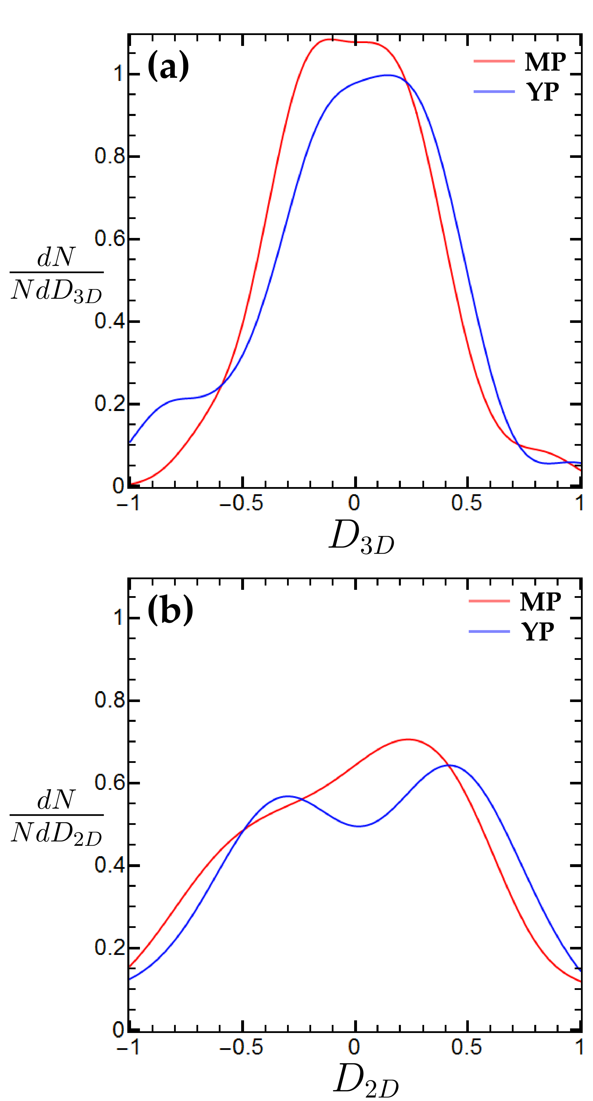
Figure 4.— (a) Smoothed out distributions of the distances $D_{\rm 3D}$ from the 3D-FP (Eq.5) for the 2PC MPs (red color) and YPs (blue color). (b) Similar to (a) but for the 2D-FP (Eq.6).

Taking into account the above, we considered a relation $L_{\gamma}=A\;B_{\star}^{b}\;\dot{\mathcal{E}}^{d}$ that excludes $\epsilon_{\rm cut}$. Then, the best-fit relation becomes

$$L_{\gamma(2D)}=10^{15.0\pm 2.6}\;B_{\star}^{0.11\pm 0.05}\;\dot{\mathcal{E}}^{0.51\pm 0.09}\leavevmode\nobreak\ .$$ (6)

In order to compare the two models, we use the Akaike information criterion (AIC; Akaike, 1974) and the Bayesian information criterion (BIC; Schwarz, 1978). Both AIC and BIC measure the goodness of the fit while they penalize the addition of extra model parameters. The lower the values of AIC and BIC the more preferable the model is. For the adopted models, the corresponding AIC, BIC values read

$$\begin{split}\rm AIC_{3D}&=159,\;\;\;\;\rm AIC_{2D}=180\\ \rm BIC_{3D}&=172,\;\;\;\;\rm BIC_{2D}=189\leavevmode\nobreak\ \end{split}$$ (7)

which indicate that the 3D model (i.e., the one that includes $\epsilon_{\rm cut}$) is strongly preferred over the 2D one although the 3D model has an additional parameter. We note that it is the difference in AIC and BIC values between the two models that is important rather than their actual values. The specific AIC difference implies that the observed sample of data is $e^{(159-180)/2}=e^{-21/2}\approx 10^{-5}$ times less probable to have been produced by the 2D model than the 3D one. For the BIC any difference greater than ten indicates a very strong evidence in favor of the model with the lower value.

In Fig.4b, we plot similarly to what we did for the 3D-plane, the distributions of the distances of the sample-points from the 2D-plane (6). We see that these distributions are not only broader than those of the 3D-model but they also deviate considerably from the Gaussian shape. We note that a relation $L_{\gamma}=A\dot{\mathcal{E}}^{d}$ provides results similar to those of relation (6).

The last approach provides an unbiased treatment in the sense that it is data-oriented and dissociated from any theoretical assumptions. Therefore, the FP, described by Eq.(5), is supported by the data and could have, in principle, been discovered without the theory guidance. Nonetheless, the almost perfect agreement with the theoretical FP, described by Eq.(B8) corresponding to the CR-regime, provides a solid description in simple terms of the physical processes that are responsible for the phenomenology of $\gamma$-ray pulsars.

In Fig.5, we reproduce the $L_{\gamma}$ vs. $\dot{\mathcal{E}}$ diagram by calculating the $L_{\gamma}$-values from the FP-relation (5). Thus, the red and blue points correspond to the YPs and MPs, respectively, and have been derived using the corresponding (observed) $B_{\star}$, $\dot{\mathcal{E}}$, and $\epsilon_{\rm cut}$ values. The black and gray points show the moving average values (five points along $\dot{\mathcal{E}}$) of 2PC for YPs and MPs, respectively. Finally, the blue (YPs) and red (MPs) lines have been derived assuming the empirical $\epsilon_{\rm cut}-\dot{\mathcal{E}}$ relations (3). The two lines (of the same color) and the shaded region between them cover the range of the different $B_{\star}$-values (i.e., $B_{\star}=10^{8}-10^{9}$G for MPs and $B_{\star}=10^{11.8}-10^{13}$G for YPs). We see that the FP-relation reproduces the observed behavior of $L_{\gamma}$ very well. Actually, it reproduces the trend of YPs having (on average) slightly higher $L_{\gamma}$-values than those of MPs for the same $\dot{\mathcal{E}}$ as well as the softening of the $L_{\gamma}$ vs. $\dot{\mathcal{E}}$ at high $\dot{\mathcal{E}}$ for the YPs.

Finally, our results indicate that for the CR-regime $E_{\rm acc}/B_{\rm LC}$ saturates towards low $\dot{\mathcal{E}}$-values (see Fig.3a and fig.2b in Kalapotharakos et al. 2017). Assuming that this trend persists for lower $\dot{\mathcal{E}}$, from Eqs.(2) and (B5) and taking into account the Eqs.(B1), (B3) for the CR-regime, we get

$$\epsilon_{\rm cut}\propto B_{\star}^{-1/8}\dot{\mathcal{E}}^{7/16}$$ (8)

which is a generalization of the eq.(A7) of Kalapotharakos et al. (2017). Taking into account the weak dependence on $B_{\star}$ and that $B_{\star}$ can be considered more or less constant for each population (YP or MP), we get $\epsilon_{\rm cut}\propto\dot{\mathcal{E}}^{7/16}$, which is not much different than the empirical behaviors (for low-$\dot{\mathcal{E}}$) reflected in the expressions in Eq.(3). The implied decrease of $\epsilon_{\rm cut}$ towards smaller $\dot{\mathcal{E}}$-values where Fermi becomes less sensitive combined with the correspondingly smaller $L_{\gamma}$ provide a viable interpretation of the (to-date) observed $\gamma$-ray pulsar death-line (see Smith et al., 2019). Equation (B8) (for the CR-regime) and Eq.(8) provide the asymptotic behavior $L_{\gamma}\propto\dot{\mathcal{E}}$, toward low-$\dot{\mathcal{E}}$. These claims could be tested and further explored with a telescope with better sensitivity in the MeV-band like AMEGO.

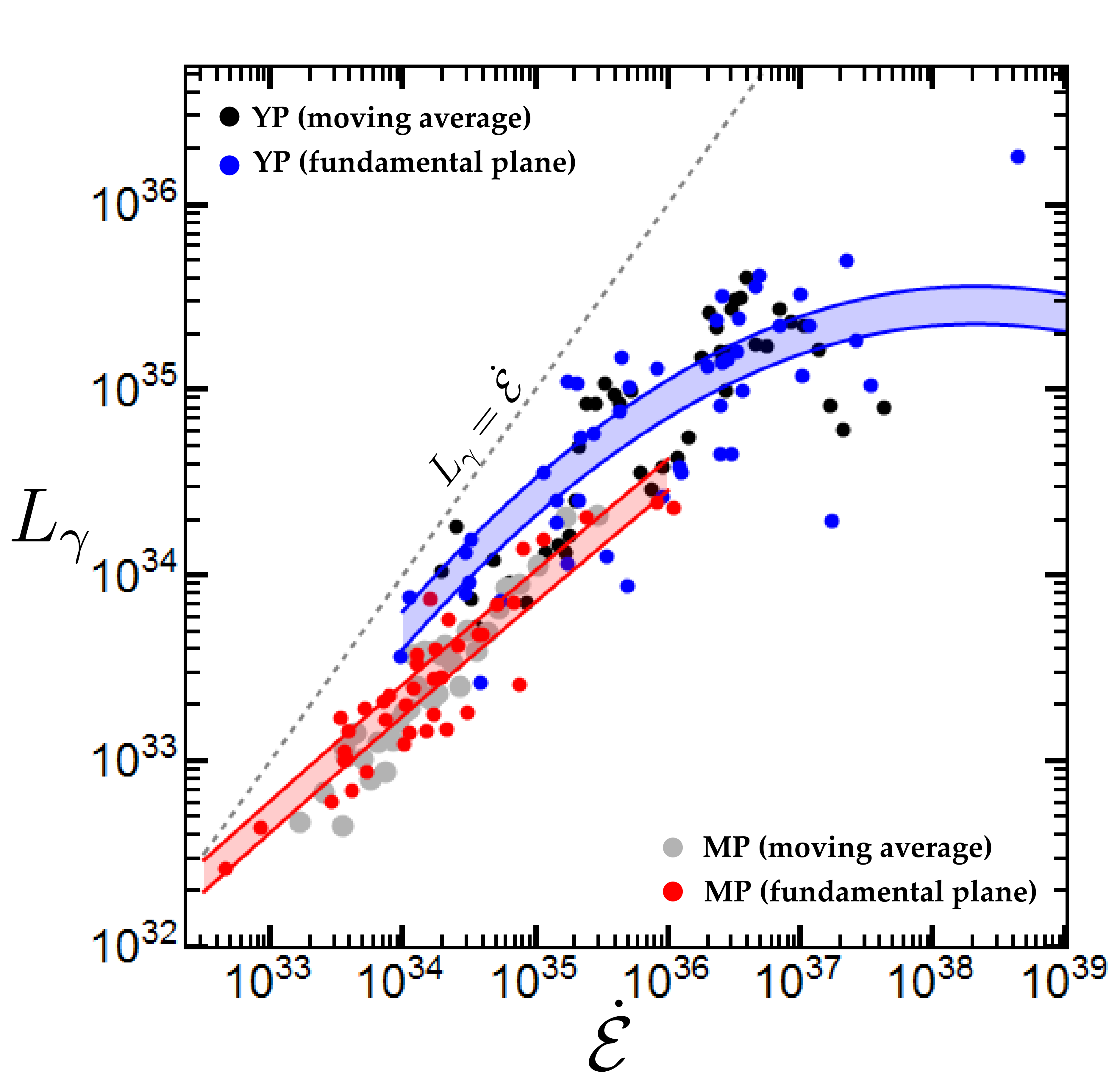
Figure 5.— The $L_{\gamma}$ vs $\dot{\mathcal{E}}$ diagram. The black and gray points denote the moving-average values of 2PC YPs and MPs, respectively. The blue (2PC-YPs) and red (2PC-MPs) points denote $L_{\gamma}$ values that have been calculated by the FP-relation (Eq.5) taking into account the observed $\dot{\mathcal{E}}$, $\epsilon_{\rm cut}$, and $B_{\star}$ values. The blue (YPs) and red (MPs) zones map the FP-relation (Eq.5) assuming that $\epsilon_{\rm cut}$ is given by Eqs.(3) and $B_{\star}$ ranges $10^{8}-10^{9}$G (for MPs) and $10^{11.8}-10^{13}$G (for YPs).

4. Discussion and Conclusions

In this letter, we explore the behavior of particle orbits, for the entire spectrum of regimes from the pure CR to the pure SR one, which are consistent with the observed photon energies, adopting the current consensus that the $\gamma$-rays are produced near the ECS. The particle $\gamma_{\rm L}$-values in the CR-regime reach up to $10^{7}-10^{8}$ while in the SR-regime and especially for the high $\dot{\mathcal{E}}$-values are 2-3 orders of magnitude lower.

Kinetic PIC models also agree with this picture. K18 demonstrated that in PIC global models, CR emission is produced by particles with realistic $\gamma_{\rm L}$-values that reach up to these levels (i.e., $10^{7}-10^{8}$). Moreover, PS18 claimed that particle emission at GeV energies is due to SR. Nonetheless, in PS18, the potential drops and the corresponding $E_{\rm acc}$ as are reflected in the presented proton energies (see fig.6 of PS18) are (scaled to the actual pulsar environment values) sufficient to support the $e^{+},e^{-}$ energies required for the CR-regime.

We have derived fundamental relations between $L_{\gamma}$, $\epsilon_{\rm cut}$, $B_{\star}$, and $\dot{\mathcal{E}}$ for the pure CR and SR assuming emission near the LC at the radiation-reaction regime. Remarkably, the Fermi-data reveal that the entire pulsar population (YPs and MPs) lie on a FP that is totally consistent with emission in the CR-regime. On the other hand, SR seems to fail at least under the assumed considerations. Even though SR may work under different conditions (e.g., acceleration and cooling may occur at different places), it seems that in such a case, a fine-tuning is needed to lock not only $E_{\rm acc}$, the acceleration lengths, the $B$-values, and the corresponding $\theta$-values where the cooling takes place but also their dependence on $\dot{\mathcal{E}}$ that reproduces the observed correlations.

The decrease of the accelerating electric fields (in $B_{\rm LC}$ units) with $\dot{\mathcal{E}}$ implies an increasing number of particles that more efficiently short-out $E_{\rm acc}$. However, our analysis shows that for CR the best agreement with observations is achieved when the number of emitting particles is scaled with the Goldreich-Julian number-density, $n_{\rm GJ\star}$. Apparently, based on our considerations in Appendix B, this implies that even though the relative particle number-density increases with $\dot{\mathcal{E}}$, the corresponding relative volume decreases in inverse proportion.

The scatter around the FP has a standard deviation $\sim 0.35$dex and is typically larger than the corresponding observational errors (mainly owing to distance measurement errors). This implies that the scatter is due to some other systematic effects. Other unknown parameters (i.e., $\alpha$, observer-angle, $\zeta$) may be responsible for the thickening of the FP. We note that the calculation of $L_{\gamma}$ in 2PC is based on the observed flux, $G_{\gamma}$, assuming that the beaming-factor $f_{\rm b}$ (see Romani & Watters 2010; 2PC) is 1 (i.e., the same) for all the detected pulsars. However, our macroscopic and kinetic PIC simulations show a variation of $f_{\rm b}$ with $\zeta$, which in combination with the various $\alpha$-values could explain the observed scatter. Therefore, the $L_{\gamma}$-values provided by 2PC, are essentially effective values, $L_{\rm\gamma\;eff}$, since they are based on the assumption that the corresponding $f_{\rm b}$ are uniformly distributed.

The theoretical analysis, presented in this letter, provides a simple physical justification of the observed FP based on the assumption that $R_{\rm C}$ is a certain fraction/multiple of the corresponding $R_{\rm LC}$, for all $\dot{\mathcal{E}}$. Nonetheless, the particle orbits corresponding to different $\alpha$ and $\zeta$ values have different $R_{\rm C}$ values. This implies that the proportionality factor between $R_{\rm C}$ and $R_{\rm LC}$ varies with $\alpha$ and $\zeta$, which consequently implies the existence of different (though parallel) FPs. Thus, the relative position of a pulsar with respect to the FP may constrain $\alpha$ and $\zeta$.

Any theoretical modeling should be able not only to reproduce the uncovered relations but also to provide justifications of the observed scatter. In a forthcoming paper, we will present under what conditions kinetic PIC models reproduce the revealed $\gamma$-ray pulsar sequence.

Appendix A The Radius of Curvature Behavior in Arbitrary Electromagnetic Field Structure

In an electromagnetic field, an asymptotic trajectory is always locally defined by the so-called Aristotelian electrodynamics (Gruzinov 2012; Kelner et al. 2015; K18)

$$\boldsymbol{\mathrm{v_{A}}}=\frac{\mathbf{E}\times\mathbf{B}\pm(B_{0}\mathbf{B}+E_{0}\mathbf{E})}{B^{2}+E_{0}^{2}}c$$ (A1)

where $E_{0}B_{0}=\mathbf{E}\cdot\mathbf{B},\;\;E_{0}^{2}-B_{0}^{2}=E^{2}-B^{2}$.

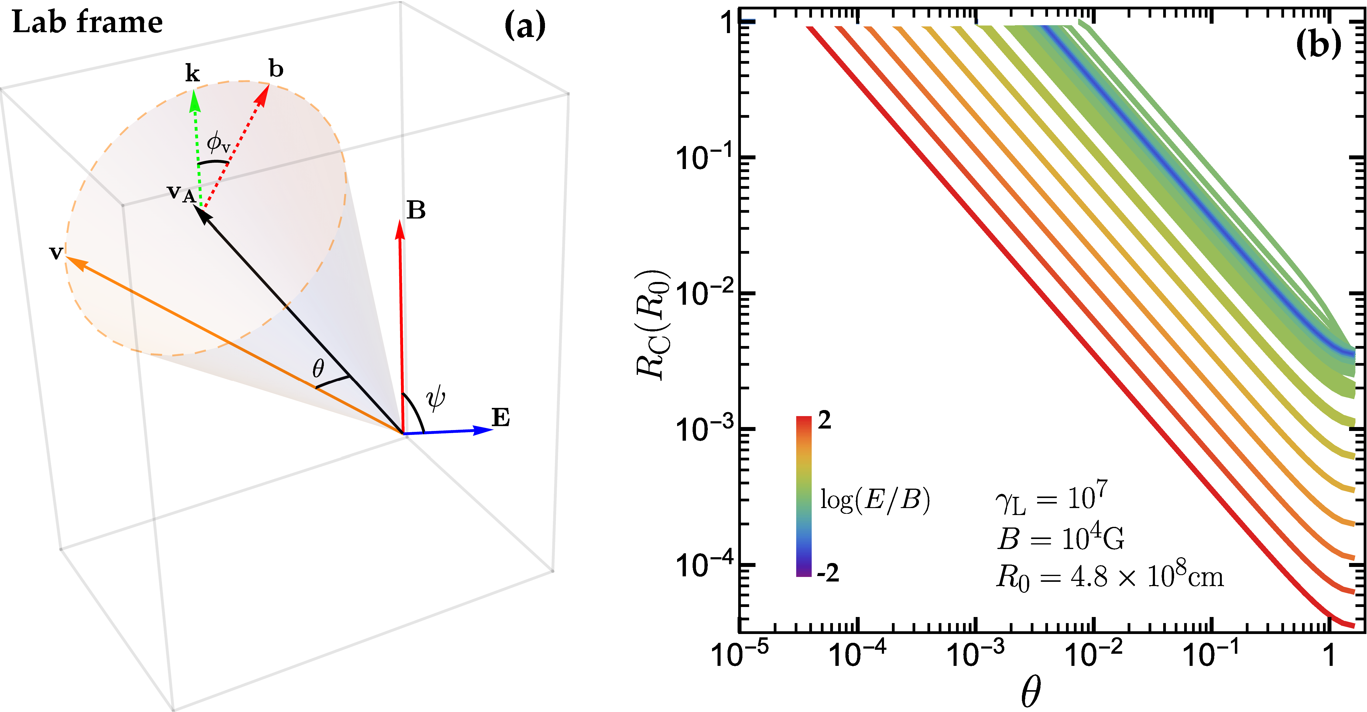
Figure 6.— (a) The relative orientation between $\mathbf{v}$ and $\mathbf{v_{A}}$ is determined by the angles $\theta$ and $\phi_{\rm v}$ where $\mathbf{b}$, $\mathbf{k}$ denote the perpendicular projection of $\mathbf{B}$ to $\mathbf{v_{A}}$ and the $\mathbf{v}\times\mathbf{v_{A}}$ direction, respectively. (b) The average (over $\phi_{\rm v}$) $R_{\rm C}$ for the indicated parameter values, $E/B$-ratio, and various $\psi$-values. For $E\ll B$ and $E\gg B$, the effect of $\psi$ is negligible (thin single color regions) while for $E\approx B$, $\psi$ slightly modulates $R_{\rm C}$ (green line zones).

The particle velocity $\mathbf{v}$ continuously approaches $\mathbf{v_{A}}$ (i.e., the generalized pitch-angle $\theta$ decreases). The particle energy loss-rate is determined by the local $R_{\rm C}={\gamma_{\rm L}m_{\rm e}c^{2}}/{(q_{e}B_{\rm eff})}$, where $\gamma_{\rm L},\leavevmode\nobreak\ m_{\rm e},\leavevmode\nobreak\ q_{\rm e}$ are the Lorentz factor, the mass, and the charge of the particle, respectively, $c$ the speed-of-light, and $B_{\rm eff}$ reads (C16)

$$B_{\rm eff}=\sqrt{(\mathbf{E}+\mathbf{v}\times\mathbf{B}/c)^{2}-(\mathbf{v}\cdot\mathbf{E}/c)^{2}}\leavevmode\nobreak\ .$$ (A2)

Figure 6a shows that $R_{\rm C}$ depends on $E,B$, the angles $\psi$, $\theta$, and the relative orientation of $\mathbf{v}$ on the $\theta$-cone (i.e., $\phi_{\rm v}$). On the one hand, the lowest $R_{\rm C}$-value, $r_{\min}$, which is achieved for high $\theta$ is mainly determined by the order of magnitude of the highest field value ($B_{\rm eff}=\max(E,B)$) while the variation of $\psi$ and $\phi_{\rm v}$ produces a modulation around a mean value (Fig.6b). On the other hand, for $\mathbf{v}=\mathbf{v_{A}}$, $B_{\rm eff}=0$. Assuming that $R_{\rm 0}$ is the $R_{\rm C}$-value corresponding to the asymptotic flow, a small velocity component perpendicular to $\mathbf{v_{A}}$ (i.e., small $\theta$) is developed that imposes $R_{\rm C}=R_{0}$. For motion near the LC, the fields are $\sim B_{\rm LC}$ and therefore $r_{\min}\sim r_{\rm g}$.

Appendix B Derivation of the Theoretical Fundamental Plane Relations

The spin-down power for a dipole field reads

$$\dot{\mathcal{E}}\propto B_{\star}^{2}P^{-4}\leavevmode\nobreak\ .$$ (B1)

Assuming

1. emission at the LC near the ECS (i.e., fields of the order of $B_{\rm LC}$) and taking into account that

   $$B_{\rm LC}\propto B_{\star}R_{\rm LC}^{-3}\propto B_{\star}P^{-3}$$ (B2)

   and $R_{\rm LC}\propto P$, we get

   $$R_{\rm C}\propto\begin{cases}R_{\rm LC}\propto P&\text{CR-regime}\\ r_{\rm g}\propto\gamma_{\rm L}P^{3}B_{\star}^{-1}&\text{SR-regime}\end{cases}$$ (B3)

   and then from Eq.(2) and (B3), we get

   $$\gamma_{\rm L}\propto\begin{cases}\epsilon_{\rm cut}^{1/3}P^{1/3}&\text{CR-regime}\\ \epsilon_{\rm cut}^{1/2}P^{3/2}B_{\star}^{-1/2}&\text{SR-regime}\end{cases}$$ (B4)

2. a balance between acceleration and radiative losses

   $$E_{\rm BLC}B_{\rm LC}\propto\gamma_{\rm L}^{4}R_{\rm C}^{-2}$$ (B5)

   where $E_{\rm BLC}$ is the $E_{\rm acc}$ in $B_{\rm LC}$ units. From Eqs.(B2)-(B5), we get

   $$E_{\rm BLC}\propto\begin{cases}\epsilon_{\rm cut}^{4/3}P^{7/3}B_{\star}^{-1}&\text{CR-regime}\\ \epsilon_{\rm cut}&\text{{SR-regime}}\end{cases}$$ (B6)

   and consequently the luminosity of one-particle reads

   $$L_{\gamma 1}\propto E_{\rm BLC}B_{\rm LC}\propto\begin{cases}\epsilon_{\rm cut}^{4/3}P^{-2/3}&\text{CR-regime}\\ \epsilon_{\rm cut}B_{\star}P^{-3}&\text{{SR-regime}}\end{cases}$$ (B7)

3. that the total $\gamma$-ray luminosity $L_{\gamma}$ scales with the number of emitting particles in the dissipative region, $N_{d}=n_{\rm GJ\mathchar 45\relax LC}\;V_{d}$, where $n_{\rm GJ\mathchar 45\relax LC}$ is the Goldreich-Julian number-density at the LC, $n_{\rm GJ\mathchar 45\relax LC}\propto n_{\rm GJ\star}R_{\rm LC}^{-3}\propto B_{\star}P^{-1}R_{\rm LC}^{-3}$ where $n_{\rm GJ\star}$ is the Goldreich-Julian number-density on the stellar surface and $V_{d}$ the volume of the dissipative region, which we assume that $V_{d}\propto R_{\rm LC}^{3}$. Thus, $N_{d}\propto n_{\rm GJ\star}\propto B_{\star}P^{-1}$ and taking into account Eq.(B1), we get

   $$L_{\gamma}\propto L_{\gamma 1}B_{\star}P^{-1}\propto\begin{cases}\epsilon_{\rm cut}^{4/3}B_{\star}^{1/6}\dot{\mathcal{E}}^{5/12}&\text{CR-regime}\\ \epsilon_{\rm cut}\;\dot{\mathcal{E}}&\text{{SR-regime}}\end{cases}$$ (B8)

We note that according to Eqs.(B1) and (B8), $L_{\gamma}$ may be a function of any 2-combinations of the $(\dot{\mathcal{E}},\leavevmode\nobreak\ B_{\star},\leavevmode\nobreak\ P)$ variable-set. Moreover, taking into account that $\dot{\mathcal{E}}\propto P^{-3}\dot{P}$, $L_{\gamma}$ may also be expressed as a function of the directly observable quantities

$$L_{\gamma}\propto\begin{cases}\epsilon_{\rm cut}^{4/3}P^{-7/6}\dot{P}^{1/2}&\text{CR-regime}\\ \epsilon_{\rm cut}\;P^{-3}\dot{P}&\text{{SR-regime}}\end{cases}$$ (B9)

Nonetheless, any of these relations are equivalent.

References

- Abdo et al. (2013) Abdo, A. A., Ajello, M., Allafort, A., et al. 2013, ApJS, 208, 17 (2PC)
- Akaike (1974) Akaike, H. 1974, IEEE Transactions on Automatic Control, 19, 716
- Ansoldi et al. (2016) Ansoldi, S., Antonelli, L. A., Antoranz, P., et al. 2016, A&A, 585, A133
- Bai & Spitkovsky (2010) Bai, X.-N., & Spitkovsky, A. 2010, ApJ, 715, 1282
- Brambilla et al. (2015) Brambilla, G., Kalapotharakos, C., Harding, A. K., & Kazanas, D. 2015, ApJ, 804, 84
- Brambilla et al. (2018) Brambilla, G., Kalapotharakos, C., Timokhin, A. N., Harding, A. K., & Kazanas, D. 2018, ApJ, 858, 81
- Cerutti et al. (2016) Cerutti, B., Philippov, A. A., & Spitkovsky, A. 2016, MNRAS, 457, 2401 (C16)
- Chen & Beloborodov (2014) Chen, A. Y., & Beloborodov, A. M. 2014, ApJ, 795, L22
- Contopoulos & Kalapotharakos (2010) Contopoulos, I., & Kalapotharakos, C. 2010, MNRAS, 404, 767
- Contopoulos et al. (1999) Contopoulos, I., Kazanas, D., & Fendt, C. 1999, ApJ, 511, 351
- Djannati-Ataï et al. (2017) Djannati-Ataï, A., Giavitto, G., Holler, M., et al. 2017, in American Institute of Physics Conference Series, Vol. 1792, 6th International Symposium on High Energy Gamma-Ray Astronomy, 040028
- Gruzinov (2012) Gruzinov, A. 2012, arXiv e-prints, arXiv:1205.3367
- Harding et al. (2018) Harding, A. K., Kalapotharakos, C., Barnard, M., & Venter, C. 2018, ApJ, 869, L18