Batched Multi-armed Bandits Problem

Abstract

In this paper, we study the multi-armed bandit problem in the batched setting where the employed policy must split data into a small number of batches. While the minimax regret for the two-armed stochastic bandits has been completely characterized in PRCS (16), the effect of the number of arms on the regret for the multi-armed case is still open. Moreover, the question whether adaptively chosen batch sizes will help to reduce the regret also remains underexplored. In this paper, we propose the BaSE (batched successive elimination) policy to achieve the rate-optimal regrets (within logarithmic factors) for batched multi-armed bandits, with matching lower bounds even if the batch sizes are determined in an adaptive manner.

1 Introduction and Main Results

Batch learning and online learning are two important aspects of machine learning, where the learner is a passive observer of a given collection of data in batch learning, while he can actively determine the data collection process in online learning. Recently, the combination of these learning procedures has been arised in an increasing number of applications, where the active querying of data is possible but limited to a fixed number of rounds of interaction. For example, in clinical trials Tho (33); Rob (52), data come in batches where groups of patients are treated simultaneously to design the next trial. In crowdsourcing KCS (08), it takes the crowd some time to answer the current queries, so that the total time constraint imposes restrictions on the number of rounds of interaction. Similar problems also arise in marketing BM (07) and simulations CG (09).

In this paper we study the influence of round constraints on the learning performance via the following batched multi-armed bandit problem. Let ${\mathcal{I}}=\{1,2,\cdots,K\}$ be a given set of $K\geq 2$ arms of a stochastic bandit, where successive pulls of an arm $i\in{\mathcal{I}}$ yields rewards which are i.i.d. samples from distribution $\nu^{(i)}$ with mean $\mu^{(i)}$. Throughout this paper we assume that the reward follows a Gaussian distribution, i.e., $\nu^{(i)}={\mathcal{N}}(\mu^{(i)},1)$, where generalizations to general sub-Gaussian rewards and variances are straightforward. Let $\mu^{\star}=\max_{i\in[K]}\mu^{(i)}$ be the expected reward of the best arm, and $\Delta_{i}=\mu^{\star}-\mu^{(i)}\geq 0$ be the gap between arm $i$ and the best arm. The entire time horizon $T$ is splitted into $M$ batches represented by a grid ${\mathcal{T}}=\{t_{1},\cdots,t_{M}\}$, with $1\leq t_{1}<t_{2}<\cdots<t_{M}=T$, where the grid belongs to one of the following categories:

1. Static grid: the grid ${\mathcal{T}}=\{t_{1},\cdots,t_{M}\}$ is fixed ahead of time, before sampling any arms;

2. Adaptive grid: for $j\in[M]$, the grid value $t_{j}$ may be determined after observing the rewards up to time $t_{j-1}$ and using some external randomness.

Note that the adaptive grid is more powerful and practical than the static one, and we recover batch learning and online learning by setting $M=1$ and $M=T$, respectively. A sampling policy $\pi=(\pi_{t})_{t=1}^{T}$ is a sequence of random variables $\pi_{t}\in[K]$ indicating which arm to pull at time $t\in[T]$, where for $t_{j-1}<t\leq t_{j}$, the policy $\pi_{t}$ depends only on observations up to time $t_{j-1}$. In other words, the policy $\pi_{t}$ only depends on observations strictly anterior to the current batch of $t$. The ultimate goal is to devise a sampling policy $\pi$ to minimize the expected cumulative regret (or pseudo-regret, or simply regret), i.e., to minimize $\mathbb{E}[R_{T}(\pi)]$ where

$$R_{T}(\pi)\triangleq\sum_{t=1}^{T}\left(\mu^{\star}-\mu^{(\pi_{t})}\right)=T\mu^{\star}-\sum_{t=1}^{T}\mu^{(\pi_{t})}.$$

Let $\Pi_{M,T}$ be the set of policies with $M$ batches and time horizon $T$, our objective is to characterize the following minimax regret and problem-dependent regret under the batched setting:

$$R_{\text{min-max}}^{\star}(K,M,T) \triangleq\inf_{\pi\in\Pi_{M,T}}\sup_{\{\mu^{(i)}\}_{i=1}^{K}:\Delta_{i}\leq\sqrt{K}}\mathbb{E}[R_{T}(\pi)],$$ (1)

$$R_{\text{pro-dep}}^{\star}(K,M,T) \triangleq\inf_{\pi\in\Pi_{M,T}}\sup_{\Delta>0}\Delta\cdot\sup_{\{\mu^{(i)}\}_{i=1}^{K}:\Delta_{i}\in\{0\}\cup[\Delta,\sqrt{K}]}\mathbb{E}[R_{T}(\pi)].$$ (2)

Note that the gaps between arms can be arbitrary in the definition of the minimax regret, while a lower bound on the minimum gaps is present in the problem-dependent regret. The constraint $\Delta_{i}\leq\sqrt{K}$ is a technical condition in both scenarios, which is more relaxed than the usual condition $\Delta_{i}\in[0,1]$. These quantities are motivated by the fact that, when $M=T$, the upper bounds of the regret for multi-armed bandits usually take the form Vog (60); LR (85); AB (09); BPR (13); PR (13)

$$\mathbb{E}[R_{T}(\pi^{1})] \leq C\sqrt{KT},$$

$$\mathbb{E}[R_{T}(\pi^{2})] \leq C\sum_{i\in[K]:\Delta_{i}>0}\frac{\max\{1,\log(T\Delta_{i}^{2})\}}{\Delta_{i}},$$

where $\pi^{1},\pi^{2}$ are some policies, and $C>0$ is an absolute constant. These bounds are also tight in the minimax sense LR (85); AB (09). As a result, in the fully adaptive setting (i.e., when $M=T$), we have the optimal regrets $R_{\text{min-max}}^{\star}(K,T,T)=\Theta(\sqrt{KT})$, and $R_{\text{pro-dep}}^{\star}(K,T,T)=\Theta(K\log T)$. The target is to find the dependence of these quantities on the number of batches $M$.

Our first result tackles the upper bounds on the minimax regret and problem-dependent regret.

Theorem 1.

For any $K\geq 2,T\geq 1,1\leq M\leq T$, there exist two policies $\pi^{1}$ and $\pi^{2}$ under static grids (explicitly defined in Section 2) such that if $\max_{i\in[K]}\Delta_{i}\leq\sqrt{K}$, we have

$$\mathbb{E}[R_{T}(\pi^{1})] \leq\mathsf{polylog}(K,T)\cdot\sqrt{K}T^{\frac{1}{2-2^{1-M}}},$$

$$\mathbb{E}[R_{T}(\pi^{2})] \leq\mathsf{polylog}(K,T)\cdot\frac{KT^{1/M}}{\min_{i\neq\star}\Delta_{i}},$$

where $\mathsf{polylog}(K,T)$ hides poly-logarithmic factors in $(K,T)$.

The following corollary is immediate.

Corollary 1.

For the $M$-batched $K$-armed bandit problem with time horizon $T$, it is sufficient to have $M=O(\log\log T)$ batches to achieve the optimal minimax regret $\Theta(\sqrt{KT})$, and $M=O\left(\log T\right)$ to achieve the optimal problem-dependent regret $\Theta(K\log T)$, where both optimal regrets are within logarithmic factors.

For the lower bounds of the regret, we treat the static grid and the adaptive grid separately. The next theorem presents the lower bounds under any static grid.

Theorem 2.

For the $M$-batched $K$-armed bandit problem with time horizon $T$ and any static grid, the minimax and problem-dependent regrets can be lower bounded as

$$R_{\text{\rm min-max}}^{\star}(K,M,T) \geq c\cdot\sqrt{K}T^{\frac{1}{2-2^{1-M}}},$$

$$R_{\text{\rm pro-dep}}^{\star}(K,M,T) \geq c\cdot KT^{\frac{1}{M}},$$

where $c>0$ is a numerical constant independent of $K,M,T$.

We observe that for any static grids, the lower bounds in Theorem 2 match those in Theorem 1 within poly-logarithmic factors. For general adaptive grids, the following theorem shows regret lower bounds which are slightly weaker than Theorem 2.

Theorem 3.

For the $M$-batched $K$-armed bandit problem with time horizon $T$ and any adaptive grid, the minimax and problem-dependent regrets can be lower bounded as

$$R_{\text{\rm min-max}}^{\star}(K,M,T) \geq cM^{-2}\cdot\sqrt{K}T^{\frac{1}{2-2^{1-M}}},$$

$$R_{\text{\rm pro-dep}}^{\star}(K,M,T) \geq cM^{-2}\cdot KT^{\frac{1}{M}},$$

where $c>0$ is a numerical constant independent of $K,M,T$.

Compared with Theorem 2, the lower bounds in Theorem 3 lose a polynomial factor in $M$ due to a larger policy space. However, since the number of batches $M$ of interest is at most $O(\log T)$ (otherwise by Corollary 1 we effectively arrive at the fully adaptive case with $M=T$), this penalty is at most poly-logarithmic in $T$. Consequently, Theorem 3 shows that for any adaptive grid, albeit conceptually more powerful, its performance is essentially no better than that of the best static grid. Specifically, we have the following corollary.

Corollary 2.

For the $M$-batched $K$-armed bandit problem with time horizon $T$ with either static or adaptive grids, it is necessary to have $M=\Omega(\log\log T)$ batches to achieve the optimal minimax regret $\Theta(\sqrt{KT})$, and $M=\Omega\left(\log T/\log\log T\right)$ to achieve the optimal problem-dependent regret $\Theta(K\log T)$, where both optimal regrets are within logarithmic factors.

In summary, the above results have completely characterized the minimax and problem-dependent regrets for batched multi-armed bandit problems, within logarithmic factors. It is an outstanding open question whether the $M^{-2}$ term in Theorem 3 can be removed using more refined arguments.

1.1 Related works

The multi-armed bandits problem is an important class of sequential optimization problems which has been extensively studied in various fields such as statistics, operations research, engineering, computer science and economics over the recent years BCB (12). In the fully adaptive scenario, the regret analysis for stochastic bandits can be found in Vog (60); LR (85); BK (97); ACBF (02); AB (09); AMS (09); AB (10); AO (10); GC (11); BPR (13); PR (13).

There is less attention on the batched setting with limited rounds of interaction. The batched setting is studied in CBDS (13) under the name of switching costs, where it is shown that $O(\log\log T)$ batches are sufficient to achieve the optimal minimax regret. For small number of batches $M$, the batched two-armed bandit problem is studied in PRCS (16), where the results of Theorems 1 and 2 are obtained for $K=2$. However, the generalization to the multi-armed case is not straightforward, and more importantly, the practical scenario where the grid is adaptively chosen based on the historic data is excluded in PRCS (16). For the multi-armed case, a different problem of finding the best $k$ arms in the batched setting has been studied in JJNZ (16); AAAK (17), where the goal is pure exploration, and the error dependence on the time horizon decays super-polynomially. We also refer to DRY (18) for a similar setting with convex bandits and best arm identification. The regret analysis for batched stochastic multi-armed bandits still remains underexplored.

We also review some literature on general computation with limited rounds of adaptivity, and in particular, on the analysis of lower bounds. In theoretical computer science, this problem has been studied under the name of parallel algorithms for certain tasks (e.g., sorting and selection) given either deterministic Val (75); BT (83); AA (88) or noisy outcomes FRPU (94); DKMR (14); BMW (16). In (stochastic) convex optimization, the information-theoretic limits are typically derived under the oracle model where the oracle can be queried adaptively NY (83); AWBR (09); Sha (13); DRY (18). However, in the previous works, one usually optimizes the sampling distribution over a fixed sample size at each step, while it is more challenging to prove lower bounds for policies which can also determine the sample size. There is one exception AAAK (17), whose proof relies on a complicated decomposition of near-uniform distributions. Hence, our technique of proving Theorem 3 is also expected to be an addition to these literatures.

1.2 Organization

The rest of this paper is organized as follows. In Section 2, we introduce the BaSE policy for general batched multi-armed bandit problems, and show that it attains the upper bounds in Theorem 1 under two specific grids. Section 3 presents the proofs of lower bounds for both the minimax and problem-dependent regrets, where Section 3.1 deals with the static grids and Section 3.2 tackles the adaptive grids. Experimental results are presented in Section 4. The auxiliary lemmas and the proof of main lemmas are deferred to supplementary materials.

1.3 Notations

For a positive integer $n$, let $[n]\triangleq\{1,\cdots,n\}$. For any finite set $A$, let $|A|$ be its cardinality. We adopt the standard asymptotic notations: for two non-negative sequences $\{a_{n}\}$ and $\{b_{n}\}$, let $a_{n}=O(b_{n})$ iff $\limsup_{n\to\infty}a_{n}/b_{n}<\infty$, $a_{n}=\Omega(b_{n})$ iff $b_{n}=O(a_{n})$, and $a_{n}=\Theta(b_{n})$ iff $a_{n}=O(b_{n})$ and $b_{n}=O(a_{n})$. For probability measures $P$ and $Q$, let $P\otimes Q$ be the product measure with marginals $P$ and $Q$. If measures $P$ and $Q$ are defined on the same probability space, we denote by $\mathsf{TV}(P,Q)=\frac{1}{2}\int|dP-dQ|$ and $D_{\text{KL}}(P\|Q)=\int dP\log\frac{dP}{dQ}$ the total variation distance and Kullback–Leibler (KL) divergences between $P$ and $Q$, respectively.

2 The BaSE Policy

In this section, we propose the BaSE policy for the batched multi-armed bandit problem based on successive elimination, as well as two choices of the static grids to prove Theorem 1.

2.1 Description of the policy

The policy that achieves the optimal regrets is essentially adapted from Successive Elimination (SE). The original version of SE was introduced in EDMM (06), and PR (13) shows that in the $M=T$ case SE achieves both the optimal minimax and problem-dependent rates. Here we introduce a batched version of SE called Batched Successive Elimination (BaSE) to handle the general case $M\leq T$.

Given a pre-specified grid ${\mathcal{T}}=\{t_{1},\cdots,t_{M}\}$, the idea of the BaSE policy is simply to explore in the first $M-1$ batches and then commit to the best arm in the last batch. At the end of each exploration batch, we remove arms which are probably bad based on past observations. Specfically, let ${\mathcal{A}}\subseteq{\mathcal{I}}$ denote the active arms that are candidates for the optimal arm, where we initialize ${\mathcal{A}}={\mathcal{I}}$ and sequentially drop the arms which are “significantly” worse than the “best” one. For the first $M-1$ batches, we pull all active arms for a same number of times (neglecting rounding issues) and eliminate some arms from ${\mathcal{A}}$ at the end of each batch. For the last batch, we commit to the arm in ${\mathcal{A}}$ with maximum average reward.

Before stating the exact algorithm, we introduce some notations. Let

$${\bar{Y}}^{i}(t)=\dfrac{1}{|\{s\leq t:\text{arm }i\text{ is pulled at time }s\}|}\sum^{t}_{s=1}Y_{s}\mathbbm{1}{\left\{\text{arm }i\text{ is pulled at time }s\right\}}$$

denote the average rewards of the arm $i$ up to time $t$, and $\gamma>0$ is a tuning parameter associated with the UCB bound. The algorithm is described in detail in Algorithm 1.

Input: Arms ${\mathcal{I}}=[K]$; time horizon $T$; number of batches $M$; grid ${\mathcal{T}}=\{t_{1},...,t_{M}\}$; tuning parameter $\gamma$.

Initialization: ${\mathcal{A}}\leftarrow{\mathcal{I}}$.

for $m\leftarrow 1$ to $M-1$ do

       (a) During the period $[t_{m-1}+1,t_{m}]$, pull an arm from ${\mathcal{A}}$ for a same number of times.

       (b) At time $t_{m}$:

       Let ${\bar{Y}}^{\max}(t_{m})=\max_{j\in{\mathcal{A}}}{\bar{Y}}^{j}(t_{m})$, and $\tau_{m}$ be the total number of pulls of each arm in ${\mathcal{A}}$.

       for $i\in{\mathcal{A}}$ do

             if ${\bar{Y}}^{\max}(t_{m})-{\bar{Y}}^{i}(t_{m})\geq\sqrt{\gamma\log(TK)/\tau_{m}}$ then

                   ${\mathcal{A}}\leftarrow{\mathcal{A}}-\{i\}$.

             end if

            

       end for

      

end for

for t $\leftarrow t_{M-1}+1$ to $T$ do

       pull arm $i_{0}$ such that $i_{0}\in\arg\max_{j\in{\mathcal{A}}}{\bar{Y}}^{j}(t_{M-1})$ (break ties arbitrarily).

end for

Output: Resulting policy $\pi$.

Algorithm 1 Batched Successive Elimination (BaSE)

Note that the BaSE algorithm is not fully specified unless the grid ${\mathcal{T}}$ is determined. Here we provide two choices of static grids which are similar to PRCS (16) as follows: let

$$u_{1}=a, \quad u_{m}=a\sqrt{u_{m-1}},\quad m=2,\cdots,M,\qquad t_{m}=\lfloor u_{m}\rfloor,\quad m\in[M],$$

$$u_{1}^{\prime}=b, \quad u_{m}^{\prime}=bu^{\prime}_{m-1},\quad m=2,\cdots,M,\qquad t_{m}^{\prime}=\lfloor u_{m}^{\prime}\rfloor,\quad m\in[M],$$

where parameters $a,b$ are chosen appropriately such that $t_{M}=t_{M}^{\prime}=T$, i.e.,

$$a=\Theta\left(T^{\frac{1}{2-2^{1-M}}}\right),\qquad b=\Theta\left(T^{\frac{1}{M}}\right).$$ (3)

For minimizing the minimax regret, we use the “minimax” grid defined by ${\mathcal{T}}_{\mathrm{minimax}}=\{t_{1},\cdots,t_{M}\}$; as for the problem-dependent regret, we use the “geometric” grid which is defined by ${\mathcal{T}}_{\mathrm{geometric}}=\{t_{1}^{\prime},\cdots,t_{M}^{\prime}\}$. We will denote by $\pi_{\text{BaSE}}^{1}$ and $\pi_{\text{BaSE}}^{2}$ the respective policies under these grids.

2.2 Regret analysis

The performance of the BaSE policy is summarized in the following theorem.

Theorem 4.

Consider an $M$-batched, $K$-armed bandit problem where the time horizon is $T$. let $\pi^{1}_{\emph{BaSE}}$ be the BaSE policy equipped with the grid ${\mathcal{T}}_{\mathrm{minimax}}$ and $\pi^{2}_{\emph{BaSE}}$ be the BaSE policy equipped with the grid ${\mathcal{T}}_{\mathrm{geometric}}$. For $\gamma\geq 12$ and $\max_{i\in[K]}\Delta_{i}=O(\sqrt{K})$, we have

$$\mathbb{E}[R_{T}(\pi^{1}_{\mathrm{BaSE}})] \leq C\log K\sqrt{\log(KT)}\cdot\sqrt{K}T^{\frac{1}{2-2^{1-M}}},$$ (4)

$$\mathbb{E}[R_{T}(\pi^{2}_{\mathrm{BaSE}})] \leq C\log K\log(KT)\cdot\frac{KT^{1/M}}{\min_{i\neq\star}\Delta_{i}},$$ (5)

where $C>0$ is a numerical constant independent of $K,M$ and $T$.

Note that Theorem 4 implies Theorem 1. In the sequel we sketch the proof of Theorem 4, where the main technical difficulity is to appropriately control the number of pulls for each arm under batch constraints, where there is a random number of active arms in ${\mathcal{A}}$ starting from the second batch. We also refer to a recent work EKMM (19) for a tighter bound on the problem-dependent regret with an adaptive grid.

Proof of Theorem 4.

For notational simplicity we assume that there are $K+1$ arms, where arm $0$ is the arm with highest expected reward (denoted as $\star$), and $\Delta_{i}=\mu_{\star}-\mu_{i}\geq 0$ for $i\in[K]$. Define the following events: for $i\in[K]$, let $A_{i}$ be the event that arm $i$ is eliminated before time $t_{m_{i}}$, where

$$m_{i}=\min\left\{j\in[M]:\text{arm }i\text{ has been pulled at least }\tau_{i}^{\star}\triangleq\frac{4\gamma\log(TK)}{\Delta_{i}^{2}}\text{ times before time }t_{j}\in{\mathcal{T}}\right\},$$

with the understanding that if the minimum does not exist, we set $m_{i}=M$ and the event $A_{i}$ occurs. Let $B$ be the event that arm $\star$ is not eliminated throughout the time horizon $T$. The final “good event" $E$ is defined as $E=(\cap_{i=1}^{K}A_{i})\cap B$. We remark that $m_{i}$ is a random variable depending on the order in which the arms are eliminated. The following lemma shows that by our choice of $\gamma\geq 12$, the good event $E$ occurs with high probability.

Lemma 1.

The event $E$ happens with probability at least $1-\frac{2}{TK}$.

The proof of Lemma 1 is postponed to the supplementary materials. By Lemma 1, the expected regret $R_{T}(\pi)$ (with $\pi=\pi_{\text{BaSE}}^{1}$ or $\pi_{\text{BaSE}}^{2}$) when the event $E$ does not occur is at most

$$\mathbb{E}[R_{T}(\pi)\mathbbm{1}(E^{c})]\leq T\max_{i\in[K]}\Delta_{i}\cdot\mathbb{P}(E^{c})=O(1).$$ (6)

Next we condition on the event $E$ and upper bound the regret $\mathbb{E}[R_{T}(\pi_{\text{BaSE}}^{1})\mathbbm{1}(E)]$ for the minimax grid ${\mathcal{T}}_{\text{minimax}}$. The analysis of the geometric grid ${\mathcal{T}}_{\text{geometric}}$ is entirely analogous, and is deferred to the supplementary materials.

For the policy $\pi_{\text{BaSE}}^{1}$, let ${\mathcal{I}}_{0}\subseteq{\mathcal{I}}$ be the (random) set of arms which are eliminated at the end of the first batch, ${\mathcal{I}}_{1}\subseteq{\mathcal{I}}$ be the (random) set of remaining arms which are eliminated before the last batch, and ${\mathcal{I}}_{2}={\mathcal{I}}-{\mathcal{I}}_{0}-{\mathcal{I}}_{1}$ be the (random) set of arms which remain in the last batch. It is clear that the total regret incurred by arms in ${\mathcal{I}}_{0}$ is at most $t_{1}\cdot\max_{i\in[K]}\Delta_{i}=O(\sqrt{K}a),$ and it remains to deal with the sets ${\mathcal{I}}_{1}$ and ${\mathcal{I}}_{2}$ separately.

For arm $i\in{\mathcal{I}}_{1}$, let $\sigma_{i}$ be the (random) number of arms which are eliminated before the arm $i$. Observe that the fraction of pullings of arm $i$ is at most $\frac{1}{K-\sigma_{i}}$ before arm $i$ is eliminated. Moreover, by the definition of $t_{m_{i}}$, we must have

$$\tau_{i}^{\star}>(\text{number of pullings of arm }i\text{ before }t_{m_{i}-1})\geq\frac{t_{m_{i}-1}}{K}\Longrightarrow\Delta_{i}\sqrt{t_{m_{i}-1}}\leq\sqrt{4\gamma K\log(TK)}.$$

Hence, the total regret incurred by pulling an arm $i\in{\mathcal{I}}_{1}$ is at most (note that $t_{j}\leq 2a\sqrt{t_{j-1}}$ for any $j=2,3,\cdots,M$ by the choice of the grid)

$$\Delta_{i}\cdot\frac{t_{m_{i}}}{K-\sigma_{i}}\leq\Delta_{i}\cdot\frac{2a\sqrt{t_{m_{i}-1}}}{K-\sigma_{i}}\leq\frac{2a\sqrt{4\gamma K\log(TK)}}{K-\sigma_{i}}.$$

Note that there are at most $t$ elements in $(\sigma_{i}:i\in{\mathcal{I}}_{1})$ which are at least $K-t$ for any $t=2,\cdots,K$, the total regret incurred by pulling arms in ${\mathcal{I}}_{1}$ is at most

$$\sum_{i\in{\mathcal{I}}_{1}}\frac{2a\sqrt{4\gamma K\log(TK)}}{K-\sigma_{i}}\leq 2a\sqrt{4\gamma K\log(TK)}\cdot\sum_{t=2}^{K}\frac{1}{t}\leq 2a\log K\sqrt{4\gamma K\log(TK)}.$$ (7)

For any arm $i\in{\mathcal{I}}_{2}$, by the previous analysis we know that $\Delta_{i}\sqrt{t_{M-1}}\leq\sqrt{4\gamma K\log(TK)}$. Hence, let $T_{i}$ be the number of pullings of arm $i$, the total regret incurred by pulling arm $i\in{\mathcal{I}}_{2}$ is at most

$$\Delta_{i}T_{i}\leq T_{i}\sqrt{\frac{4\gamma K\log(TK)}{t_{M-1}}}\leq\frac{T_{i}}{T}\cdot 2a\sqrt{4\gamma K\log(TK)},$$

where in the last step we have used that $T=t_{M}\leq 2a\sqrt{t_{M-1}}$ in the minimax grid ${\mathcal{T}}_{\text{minimax}}$. Since $\sum_{i\in{\mathcal{I}}_{2}}T_{i}\leq T$, the total regret incurred by pulling arms in ${\mathcal{I}}_{2}$ is at most

$$\sum_{i\in{\mathcal{I}}_{2}}\frac{T_{i}}{T}\cdot 2a\sqrt{4\gamma K\log(TK)}\leq 2a\sqrt{4\gamma K\log(TK)}.$$ (8)

By (7) and (8), the inequality

$$R_{T}(\pi_{\text{BaSE}}^{1})\mathbbm{1}(E)\leq 2a\sqrt{4\gamma K\log(TK)}(\log K+1)+O(\sqrt{K}a)$$

holds almost surely. Hence, this inequality combined with (6) and the choice of $a$ in (3) yields the desired upper bound (4). ∎

3 Lower Bound

This section presents lower bounds for the batched multi-armed bandit problem, where in Section 3.1 we design a fixed multiple hypothesis testing problem to show the lower bound for any policies under static grids, while in Section 3.2 we construct different hypotheses for different policies under general adaptive grids.

3.1 Static grid

The proof of Theorem 2 relies on the following lemma.

Lemma 2.

For any static grid $0=t_{0}<t_{1}<\cdots<t_{M}=T$ and the smallest gap $\Delta\in(0,\sqrt{K}]$, the following minimax lower bound holds for any policy $\pi$ under this grid:

$$\sup_{\{\mu^{(i)}\}_{i=1}^{K}:\Delta_{i}\in\{0\}\cup[\Delta,\sqrt{K}]}\mathbb{E}[R_{T}(\pi)]\geq\Delta\cdot\sum_{j=1}^{M}\frac{t_{j}-t_{j-1}}{4}\exp\left(-\frac{2t_{j-1}\Delta^{2}}{K-1}\right).$$

We first show that Lemma 2 implies Theorem 2 by choosing the smallest gap $\Delta>0$ appropriately. By definitions of the minimax regret $R_{\text{min-max}}^{\star}$ and the problem-dependent regret $R_{\text{pro-dep}}^{\star}$, choosing $\Delta=\Delta_{j}=\sqrt{(K-1)/(t_{j-1}+1)}\in[0,\sqrt{K}]$ in Lemma 2 yields that

$$R_{\text{min-max}}^{\star}(K,M,T) \geq c_{0}\sqrt{K}\cdot\max_{j\in[M]}\frac{t_{j}}{\sqrt{t_{j-1}+1}},$$

$$R_{\text{pro-dep}}^{\star}(K,M,T) \geq c_{0}K\cdot\max_{j\in[M]}\frac{t_{j}}{t_{j-1}+1},$$

for some numerical constant $c_{0}>0$. Since $t_{0}=0,t_{M}=T$, the lower bounds in Theorem 2 follow.

Next we employ the general idea of the multiple hypothesis testing to prove Lemma 2. Consider the following $K$ candidate reward distributions:

$$P_{1} ={\mathcal{N}}(\Delta,1)\otimes{\mathcal{N}}(0,1)\otimes{\mathcal{N}}(0,1)\otimes\cdots\otimes{\mathcal{N}}(0,1),$$

$$P_{2} ={\mathcal{N}}(\Delta,1)\otimes{\mathcal{N}}(2\Delta,1)\otimes{\mathcal{N}}(0,1)\otimes\cdots\otimes{\mathcal{N}}(0,1),$$

$$P_{3} ={\mathcal{N}}(\Delta,1)\otimes{\mathcal{N}}(0,1)\otimes{\mathcal{N}}(2\Delta,1)\otimes\cdots\otimes{\mathcal{N}}(0,1),$$

$$\qquad\qquad\qquad\qquad\qquad\quad\vdots$$

$$P_{K} ={\mathcal{N}}(\Delta,1)\otimes{\mathcal{N}}(0,1)\otimes{\mathcal{N}}(0,1)\otimes\cdots\otimes{\mathcal{N}}(2\Delta,1).$$

We remark that this construction is not entirely symmetric, where the reward distribution of the first arm is always ${\mathcal{N}}(\Delta,1)$. The key properties of this construction are as follows:

1. For any $i\in[K]$, arm $i$ is the optimal arm under reward distribution $P_{i}$;

2. For any $i\in[K]$, pulling a wrong arm incurs a regret at least $\Delta$ under reward distribution $P_{i}$.

As a result, since the average regret serves as a lower bound of the worst-case regret, we have

$$\sup_{\{\mu^{(i)}\}_{i=1}^{K}:\Delta_{i}\in\{0\}\cup[\Delta,\sqrt{K}]}\mathbb{E}R_{T}(\pi)\geq\frac{1}{K}\sum_{i=1}^{K}\sum_{t=1}^{T}\mathbb{E}_{P_{i}^{t}}R^{t}(\pi)\geq\Delta\sum_{t=1}^{T}\frac{1}{K}\sum_{i=1}^{K}P_{i}^{t}(\pi_{t}\neq i),$$ (9)

where $P_{i}^{t}$ denotes the distribution of observations available at time $t$ under $P_{i}$, and $R^{t}(\pi)$ denotes the instantaneous regret incurred by the policy $\pi_{t}$ at time $t$. Hence, it remains to lower bound the quantity $\frac{1}{K}\sum_{i=1}^{K}P_{i}^{t}(\pi_{t}\neq i)$ for any $t\in[T]$, which is the subject of the following lemma.

Lemma 3.

Let $Q_{1},\cdots,Q_{n}$ be probability measures on some common probability space $(\Omega,{\mathcal{F}})$, and $\Psi:\Omega\to[n]$ be any measurable function (i.e., test). Then for any tree $T=([n],E)$ with vertex set $[n]$ and edge set $E$, we have

$$\frac{1}{n}\sum_{i=1}^{n}Q_{i}(\Psi\neq i)\geq\sum_{(i,j)\in E}\frac{1}{2n}\exp(-D_{\text{\rm KL}}(Q_{i}\|Q_{j})).$$

The proof of Lemma 3 is deferred to the supplementary materials, and we make some remarks below.

Remark 1.

A more well-known lower bound for $\frac{1}{n}\sum_{i=1}^{n}Q_{i}(\Psi\neq i)$ is the Fano’s inequality CT (06), which involves the mutual information $I(U;X)$ with $U\sim\mathsf{Uniform}([n])$ and $P_{X|U=i}=Q_{i}$. However, since $I(U;X)=\mathbb{E}_{P_{U}}D_{\text{\rm KL}}(P_{X|U}\|P_{X})$, Fano’s inequality gives a lower bound which depends linearly on the pairwise KL divergence rather than exponentially and is thus loose for our purpose.

Remark 2.

An alternative lower bound is to use $\frac{1}{2n^{2}}\sum_{i\neq j}\exp(-D_{\text{\rm KL}}(Q_{i}\|Q_{j}))$, i.e., the summation is taken over all pairs $(i,j)$ instead of just the edges in a tree. However, this bound is weaker than Lemma 3, and in the case where $Q_{i}={\mathcal{N}}(i\Delta,1)$ for some large $\Delta>0$, Lemma 3 with the tree $T=([n],\{(1,2),(2,3),\cdots,(n-1,n)\})$ is tight (giving the rate $(\exp(-O(\Delta^{2}))$) while the alternative bound loses a factor of $n$ (giving the rate $\exp(-O(\Delta^{2}))/n$).

To lower bound (9), we apply Lemma 3 with the star tree $T=([n],\{(1,i):2\leq i\leq n\})$. For $i\in[K]$, denote by $T_{i}(t)$ the number of pulls of arm $i$ anterior to the current batch of $t$. Hence, $\sum_{i=1}^{K}T_{i}(t)=t_{j-1}$ if $t\in(t_{j-1},t_{j}]$. Moreover, since $D_{\text{KL}}(P_{1}^{t}\|P_{i}^{t})=2\Delta^{2}\mathbb{E}_{P_{1}^{t}}T_{i}(t)$, we have

$$\frac{1}{K}\sum_{i=1}^{K}P_{i}^{t}(\pi_{t}\neq i) \geq\frac{1}{2K}\sum_{i=2}^{K}\exp(-D_{\text{KL}}(P_{1}^{t}\|P_{i}^{t}))=\frac{1}{2K}\sum_{i=2}^{K}\exp(-2\Delta^{2}\mathbb{E}_{P_{1}^{t}}T_{i}(t))$$

$$\geq\frac{K-1}{2K}\exp\left(-\frac{2\Delta^{2}}{K-1}\mathbb{E}_{P_{1}^{t}}\sum_{i=2}^{K}T_{i}(t)\right)\geq\frac{1}{4}\exp\left(-\frac{2\Delta^{2}t_{j-1}}{K-1}\right).$$ (10)

Now combining (9) and (10) completes the proof of Lemma 2.

3.2 Adaptive grid

Now we investigate the case where the grid may be randomized, and be generated sequentially in an adaptive manner. Recall that in the previous section, we construct multiple fixed hypotheses and show that no policy under a static grid can achieve a uniformly small regret under all hypotheses. However, this argument breaks down even if the grid is only randomized but not adaptive, due to the non-convex (in $(t_{1},\cdots,t_{M})$) nature of the lower bound in Lemma 2. In other words, we might not hope for a single fixed multiple hypothesis testing problem to work for all policies. To overcome this difficulty, a subroutine in the proof of Theorem 3 is to construct appropriate hypotheses after the policy is given (cf. the proof of Lemma 4). We sketch the proof below.

We shall only prove the lower bound for the minimax regret, where the analysis of the problem-dependent regret is entirely analogous. Consider the following time $T_{1},\cdots,T_{M}\in[1,T]$ and gaps $\Delta_{1},\cdots,\Delta_{M}\in(0,\sqrt{K}]$ with

$$T_{j}=\lfloor T^{\frac{1-2^{-j}}{1-2^{-M}}}\rfloor,\qquad\Delta_{j}=\frac{\sqrt{K}}{36M}\cdot T^{-\frac{1-2^{1-j}}{2(1-2^{-M})}},\qquad j\in[M].$$ (11)

Let ${\mathcal{T}}=\{t_{1},\cdots,t_{M}\}$ be any adaptive grid, and $\pi$ be any policy under the grid ${\mathcal{T}}$. For each $j\in[M]$, we define the event $A_{j}=\{t_{j-1}<T_{j-1},t_{j}\geq T_{j}\}$ under policy $\pi$ with the convention that $t_{0}=0,t_{M}=T$. Note that the events $A_{1},\cdots,A_{M}$ form a partition of the entire probability space. We also define the following family of reward distributions: for $j\in[M-1],k\in[K-1]$ let

$$P_{j,k}={\mathcal{N}}(0,1)\otimes\cdots\otimes{\mathcal{N}}(0,1)\otimes{\mathcal{N}}(\Delta_{j}+\Delta_{M},1)\otimes{\mathcal{N}}(0,1)\otimes\cdots\otimes{\mathcal{N}}(0,1)\otimes{\mathcal{N}}(\Delta_{M},1),$$

where the $k$-th component of $P_{j,k}$ has a non-zero mean. For $j=M$, we define

$$P_{M}={\mathcal{N}}(0,1)\otimes\cdots\otimes{\mathcal{N}}(0,1)\otimes{\mathcal{N}}(\Delta_{M},1).$$

Note that this construction ensures that $P_{j,k}$ and $P_{M}$ only differs in the $k$-th component, which is crucial for the indistinguishability results in Lemma 5.

We will be interested in the following quantities:

$$p_{j}=\frac{1}{K-1}\sum_{k=1}^{K-1}P_{j,k}(A_{j}),\quad j\in[M-1],\qquad p_{M}=P_{M}(A_{M}),$$

where $P_{j,k}(A)$ denotes the probability of the event $A$ given the true reward distribution $P_{j,k}$ and the policy $\pi$. The importance of these quantities lies in the following lemmas.

Lemma 4.

If $p_{j}\geq\frac{1}{2M}$ for some $j\in[M]$, then we have

$$\sup_{\{\mu^{(i)}\}_{i=1}^{K}:\Delta_{i}\leq\sqrt{K}}\mathbb{E}[R_{T}(\pi)]\geq cM^{-2}\cdot\sqrt{K}T^{\frac{1}{2-2^{1-M}}},$$

where $c>0$ is a numerical constant independent of $(K,M,T)$ and $(\pi,{\mathcal{T}})$.

Lemma 5.

The following inequality holds: $\sum_{j=1}^{M}p_{j}\geq\frac{1}{2}.$

The detailed proofs of Lemma 4 and Lemma 5 are deferred to the supplementary materials, and we only sketch the ideas here. Lemma 4 states that, if any of the events $A_{j}$ occurs with a non-small probability in the respective $j$-th world (i.e., under the mixture of $(P_{j,k}:k\in[K-1])$ or $P_{M}$), then the policy $\pi$ has a large regret in the worst case. The intuition behind Lemma 4 is that, if the event $t_{j-1}\leq T_{j-1}$ occurs under the reward distribution $P_{j,k}$, then the observations in the first $(j-1)$ batches are not sufficient to distinguish $P_{j,k}$ from its (carefully designed) perturbed version with size of perturbation $\Delta_{j}$. Furthermore, if in addition $t_{j}\geq T_{j}$ holds, then the total regret is at least $\Omega(T_{j}\Delta_{j})$ due to the indistinguishability of the $\Delta_{j}$ perturbations in the first $j$ batches. Hence, if $A_{j}$ occurs with a fairly large probability, the resulting total regret will be large as well.

Lemma 5 complements Lemma 4 by stating that at least one $p_{j}$ should be large. Note that if all $p_{j}$ were defined in the same world, the partition structure of $A_{1},\cdots,A_{M}$ would imply $\sum_{j\in[M]}p_{j}\geq 1$. Since the occurrence of $A_{j}$ cannot really help to distinguish the $j$-th world with later ones, Lemma 5 shows that we may still operate in the same world and arrive at a slightly smaller constant than $1$.

Finally we show how Lemma 4 and Lemma 5 imply Theorem 3. In fact, by Lemma 5, there exists some $j\in[M]$ such that $p_{j}\geq(2M)^{-1}$. Then by Lemma 4 and the arbitrariness of $\pi$, we arrive at the desired lower bound in Theorem 3.

4 Experiments

This section contains some experimental results on the performances of BaSE policy under different grids. The default parameters are $T=5\times 10^{4},K=3,M=3$ and $\gamma=1$, and the mean reward is $\mu^{\star}=0.6$ for the optimal arm and is $\mu=0.5$ for all other arms. In addition to the minimax and geometric grids, we also experiment on the arithmetic grid with $t_{j}=jT/M$ for $j\in[M]$. Figure 1 (a)-(c) display the empirical dependence of the average BaSE regrets under different grids, together with the comparison with the centralized UCB1 algorithm ACBF (02) without any batch constraints. We observe that the minimax grid typically results in a smallest regret among all grids, and $M=4$ batches appear to be sufficient for the BaSE performance to approach the centralized performance. We also compare our BaSE algorithm with the ETC algorithm in PRCS (16) for the two-arm case, and Figure 1 (d) shows that BaSE achieves lower regrets than ETC. The source codes of the experiment can be found in https://github.com/Mathegineer/batched-bandit.

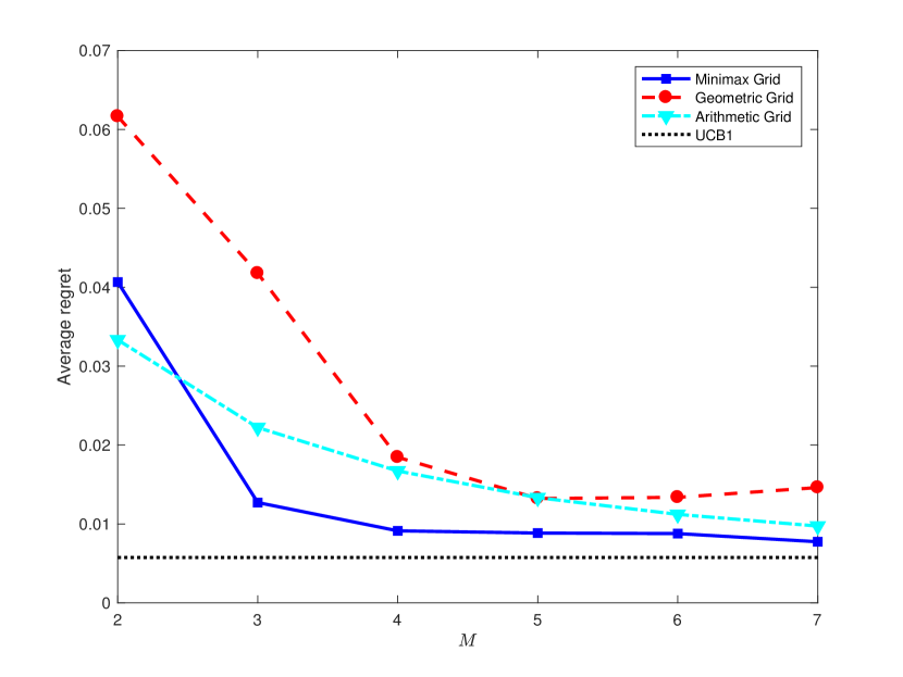
(a) Average regret vs. the number of batches $M$.

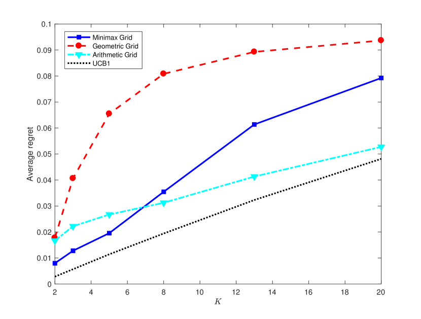
(b) Average regret vs. the number of arms $K$.

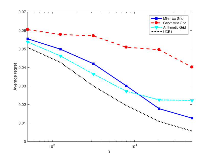
(c) Average regret vs. the time horizon $T$.

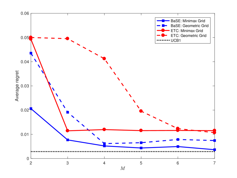
(d) Comparison of BaSE and ETC.

Figure 1: Empirical regret performances of the BaSE policy.

Appendix A Auxiliary Lemmas

The following lemma is a generalization of [33, Lemma 2.6].

Lemma 6.

Let $P$ and $Q$ be any probability measures on the same probability space. Then

$$\mathsf{TV}(P,Q)\leq\sqrt{1-\exp(-D_{\text{\rm KL}}(P\|Q))}\leq 1-\frac{1}{2}\exp\left(-D_{\text{\rm KL}}(P\|Q)\right).$$

Proof.

Observe that the proof of [33, Lemma 2.6] gives

$$\left(\int\min\{dP,dQ\}\right)\left(\int\max\{dP,dQ\}\right)\geq\exp\left(-D_{\text{KL}}(P\|Q)\right).$$

Since

$$\int\min\{dP,dQ\} =1-\mathsf{TV}(P,Q),$$

$$\int\max\{dP,dQ\} =1+\mathsf{TV}(P,Q),$$

the first inequality follows. The second inequality follows from the basic inequality $\sqrt{1-x}\leq 1-x/2$ for any $x\in[0,1]$. ∎

The following lemma presents a graph-theoretic inequality, which is the crux of Lemma 3.

Lemma 7.

Let $T=(V,E)$ be a tree on $V=[n]$, and $x\in\mathbb{R}^{n}$ be any vector. Then

$$\sum_{i=1}^{n}x_{i}-\max_{i\in[n]}x_{i}\geq\sum_{(i,j)\in E}\min\{x_{i},x_{j}\}.$$

Proof.

Without loss of generality we assume that $x_{1}\leq x_{2}\leq\cdots\leq x_{n}$. For any $k\in[n-1]$, we have

$$\sum_{(i,j)\in E}\mathbbm{1}(\min\{x_{i},x_{j}\}\geq x_{k})=|\{(i,j)\in E:i\geq k,j\geq k\}|\leq n-k,$$

where the last inequality is due to the fact that restricting the tree $T$ on the vertices $\{k,k+1,\cdots,n\}$ is still acyclic. Hence,

$$\sum_{i=1}^{n}x_{i}-\max_{i\in[n]}x_{i}=\sum_{i=1}^{n-1}x_{i} =(n-1)x_{1}+\sum_{k=2}^{n-1}(n-k)(x_{k}-x_{k-1})$$

$$\geq(n-1)x_{1}+\sum_{k=2}^{n-1}(x_{k}-x_{k-1})\sum_{(i,j)\in E}\mathbbm{1}(\min\{x_{i},x_{j}\}\geq x_{k})$$

$$=\sum_{(i,j)\in E}\left(x_{1}+\sum_{k=2}^{n-1}(x_{k}-x_{k-1})\mathbbm{1}(\min\{x_{i},x_{j}\}\geq x_{k})\right)$$

$$=\sum_{(i,j)\in E}\min\{x_{i},x_{j}\},$$

where we have used that $|E|=n-1$ for any tree. ∎

Appendix B Proof of Main Lemmas

B.1 Proof of Lemma 1

Recall that the event $E$ is defined as $E=(\cap_{i=1}^{K}A_{i})\cap B$. First we prove that $\mathbb{P}(B^{c})$ is small. Observe that if the optimal arm $\star$ is eliminated by arm $i$ at time $t$, then before time $t$ both arms are pulled the same number of times $\tau$. For any fixed realization of $\tau$, this occurs with probability at most

$$\mathbb{P}\left({\mathcal{N}}(-\Delta_{i},2\tau^{-1})\geq\sqrt{\frac{\gamma\log(TK)}{\tau}}\right)\leq\mathbb{P}\left({\mathcal{N}}(0,2\tau^{-1})\geq\sqrt{\frac{\gamma\log(TK)}{\tau}}\right)\leq\frac{1}{(TK)^{3}}.$$

As a result, by the union bound,

$$\mathbb{P}(B^{c})\leq\sum_{i=1}^{K}\sum_{t=1}^{T}\sum_{1\leq\tau\leq T}\mathbb{P}\left(\text{arm }\star\text{ is eliminated by arm }i\text{ at time }t\text{ with }\tau\text{ pulls}\right)\leq\frac{1}{TK}.$$ (12)

Next we upper bound $\mathbb{P}(B\cap A_{i}^{c})$ for any $i\in[K]$. Note that the event $B\cap A_{i}^{c}$ implies that the optimal arm $\star$ does not eliminate arm $i$ at time $t_{m_{i}}\in{\mathcal{T}}$, where both arms have been pulled $\tau\geq\tau_{i}^{\star}$ times. By the definition of $\tau_{i}^{\star}$, this implies that

$$\Delta_{i}\geq 2\sqrt{\frac{\gamma\log(TK)}{\tau}}.$$

Hence, for any fixed realizations $t_{m_{i}}$ and $\tau$, this event occurs with probability at most

$$\mathbb{P}\left({\mathcal{N}}(\Delta_{i},2\tau^{-1})\leq\sqrt{\frac{\gamma\log(TK)}{\tau}}\right)\leq\mathbb{P}\left({\mathcal{N}}(0,2\tau^{-1})\leq-\sqrt{\frac{\gamma\log(TK)}{\tau}}\right)\leq\frac{1}{(TK)^{3}}.$$

Therefore, by a union bound,

$$\mathbb{P}(B\cap A_{i}^{c}) \leq\sum_{t_{m_{i}}\in{\mathcal{T}}}\sum_{1\leq\tau\leq T}\mathbb{P}(\text{arm }\star\text{ does not eliminate arm }i\text{ at time }t_{m_{i}}\in{\mathcal{T}}\text{ with }\tau\text{ pulls})$$

$$\leq\frac{1}{TK^{2}}.$$ (13)

Combining (12) and (13), we conclude that

$$\mathbb{P}(E^{c})\leq\mathbb{P}(B^{c})+\sum_{i=1}^{K}\mathbb{P}(B\cap A_{i}^{c})\leq\frac{2}{TK}.$$

B.2 Deferred proof of Theorem 4

The regret analysis of the policy $\pi_{\text{BaSE}}^{2}$ under the geometric grid is analogous to Section 2.2. Partition the arms ${\mathcal{I}}={\mathcal{I}}_{0}\cup{\mathcal{I}}_{1}\cup{\mathcal{I}}_{2}$ as before, and let $\Delta=\min\{\Delta_{i}:i\in[K],\Delta_{i}>0\}$ be the smallest gap. We treat ${\mathcal{I}}_{0},{\mathcal{I}}_{1}$ and ${\mathcal{I}}_{2}$ separately.

1. The total regret incurred by arms in ${\mathcal{I}}_{0}$ is at most

   $$b\cdot\max_{i\in[K]}\Delta_{i}=O(b\sqrt{K})=O\left(\frac{bK}{\Delta}\right).$$ (14)

2. The total regret incurred by pulling an arm $i\in{\mathcal{I}}_{1}$ is at most

   $$\Delta_{i}\cdot\frac{t^{\prime}_{m_{i}}}{K-\sigma_{i}}\leq\frac{1}{\Delta}\cdot\frac{t^{\prime}_{m_{i}}\Delta_{i}^{2}}{K-\sigma_{i}}\leq\frac{2b}{\Delta}\cdot\frac{t^{\prime}_{m_{i}-1}\Delta_{i}^{2}}{K-\sigma_{i}}\leq\frac{2b}{\Delta}\cdot\frac{4\gamma K\log(KT)}{K-\sigma_{i}},$$

   where for the last inequality we have used the definition of $m_{i}$. Using a similar argument for $(\sigma_{i}:i\in{\mathcal{I}}_{1})$ as in Section 2.2, the total regret incurred by pulling arms in ${\mathcal{I}}_{2}$ is at most

   $$\sum_{i\in{\mathcal{I}}_{1}}\frac{2b}{\Delta}\cdot\frac{4\gamma K\log(TK)}{K-\sigma_{i}}\leq\frac{8\gamma bK\log K\log(KT)}{\Delta}.$$ (15)

3. The total regret incurred by pulling an arm $i\in{\mathcal{I}}_{2}$ (which is pulled $T_{i}$ times) is at most

   $$\Delta_{i}T_{i}\leq\frac{\Delta_{i}^{2}T_{i}}{\Delta}\leq\frac{4\gamma K\log(TK)}{\Delta}\cdot\frac{T_{i}}{t^{\prime}_{M-1}}\leq\frac{8\gamma bK\log(TK)}{\Delta}\cdot\frac{T_{i}}{T},$$

   and thus the total regret by pulling arms in ${\mathcal{I}}_{2}$ is at most

   $$\sum_{i\in{\mathcal{I}}_{2}}\frac{8\gamma bK\log(TK)}{\Delta}\cdot\frac{T_{i}}{T}\leq\frac{8\gamma bK\log(TK)}{\Delta}.$$ (16)

Now combining (14) to (16) together with the inequality (6) and the choice of $b$ in (3), we arrive at the desired upper bound (5).

B.3 Proof of Lemma 3

It is easy to show that the minimizer of $\frac{1}{n}\sum_{i=1}^{n}Q_{i}(\Psi\neq i)$ is $\Psi^{\star}(\omega)=\arg\max_{i\in[n]}Q_{i}(d\omega)$, and thus

$$\frac{1}{n}\sum_{i=1}^{n}Q_{i}(\Psi\neq i)\geq 1-\frac{1}{n}\int\max\{dQ_{1},dQ_{2},\cdots,dQ_{n}\}=\frac{1}{n}\int\left[\sum_{i=1}^{n}dQ_{i}-\max_{i\in[n]}dQ_{i}\right].$$

By Lemmas 6 and 7, we further have

$$\frac{1}{n}\sum_{i=1}^{n}Q_{i}(\Psi\neq i) \geq\sum_{(i,j)\in E}\frac{1}{n}\int\min\{dQ_{i},dQ_{j}\}$$

$$=\sum_{(i,j)\in E}\frac{1-\mathsf{TV}(Q_{i},Q_{j})}{n}$$

$$\geq\sum_{(i,j)\in E}\frac{1}{2n}\exp(-D_{\text{\rm KL}}(Q_{i}\|Q_{j})),$$

as claimed.

B.4 Proof of Lemma 4

The proof of Lemma 4 relies on the reduction of the minimax lower bound to multiple hypothesis testing. Without loss of generality we assume that $j\in[M-1]$; the case where $j=M$ is analogous. For any $k\in[K-1]$, consider the following family ${\mathcal{P}}_{j,k}=(Q_{j,k,\ell})_{\ell\in[K]}$ of reward distributions: define $Q_{j,k,k}=P_{j,k}$, and for $\ell\neq k$, let $Q_{j,k,\ell}$ be the modification of $P_{j,k}$ where the quantity $3\Delta_{j}$ is added to the mean of the $\ell$-th component of $P_{j,k}$. We have the following observations:

1. For each $\ell\in[K]$, arm $\ell$ is the optimal arm under reward distribution $Q_{j,k,\ell}$;

2. For each $\ell\in[K]$, pulling an arm $\ell^{\prime}\neq\ell$ incurs a regret at least $\Delta_{j}$ under reward distribution $Q_{j,k,\ell}$;

3. For each $\ell\neq k$, the distributions $Q_{j,k,\ell}$ and $Q_{j,k,k}$ only differ in the $\ell$-th component.

By the first two observations, similar arguments in (9) yield to

$$\sup_{\{\mu^{(i)}\}_{i=1}^{K}:\Delta_{i}\leq\sqrt{K}}\mathbb{E}[R_{T}(\pi)]\geq\Delta_{j}\sum_{t=1}^{T}\frac{1}{K}\sum_{\ell=1}^{K}Q_{j,k,\ell}^{t}(\pi_{t}\neq\ell),$$

where $Q_{j,k,\ell}^{t}$ denotes the distribution of observations available at time $t$ under reward distribution $Q_{j,k,\ell}$, and $\pi_{t}$ denotes the policy at time $t$. We lower bound the above quantity as

$$\sup_{\{\mu^{(i)}\}_{i=1}^{K}:\Delta_{i}\leq\sqrt{K}}\mathbb{E}[R_{T}(\pi)] \overset{\rm(a)}{\geq}\Delta_{j}\sum_{t=1}^{T}\frac{1}{K}\sum_{\ell\neq k}\int\min\{dQ_{j,k,k}^{t},dQ_{j,k,\ell}^{t}\}$$

$$\geq\Delta_{j}\sum_{t=1}^{T_{j}}\frac{1}{K}\sum_{\ell\neq k}\int\min\{dQ_{j,k,k}^{t},dQ_{j,k,\ell}^{t}\}$$

$$\overset{\rm(b)}{\geq}\Delta_{j}T_{j}\cdot\frac{1}{K}\sum_{\ell\neq k}\int\min\{dQ_{j,k,k}^{T_{j}},dQ_{j,k,\ell}^{T_{j}}\}$$

$$\geq\Delta_{j}T_{j}\cdot\frac{1}{K}\sum_{\ell\neq k}\int_{A_{j}}\min\{dQ_{j,k,k}^{T_{j}},dQ_{j,k,\ell}^{T_{j}}\}$$

$$\overset{\rm(c)}{=}\Delta_{j}T_{j}\cdot\frac{1}{K}\sum_{\ell\neq k}\int_{A_{j}}\min\{dQ_{j,k,k}^{T_{j-1}},dQ_{j,k,\ell}^{T_{j-1}}\},$$ (17)

where (a) follows by the proof of Lemma 3 and considering a star graph on $[K]$ with center $k$, and (b) is due to the identity $\int\min\{dP,dQ\}=1-\mathsf{TV}(P,Q)$ and the data processing inequality of the total variation distance, and for step (c) we note that when $A_{j}=\{t_{j-1}<T_{j-1},t_{j}\geq T_{j}\}$ holds, the observations seen by the policy at time $T_{j}$ are the same as those seen at time $T_{j-1}$. To lower bound the final quantity, we further have

$$\int_{A_{j}}\min\{dQ_{j,k,k}^{T_{j-1}},dQ_{j,k,\ell}^{T_{j-1}}\} =\int_{A_{j}}\frac{dQ_{j,k,k}^{T_{j-1}}+dQ_{j,k,\ell}^{T_{j-1}}-|dQ_{j,k,k}^{T_{j-1}}-dQ_{j,k,\ell}^{T_{j-1}}|}{2}$$

$$=\frac{Q_{j,k,k}^{T_{j-1}}(A_{j})+Q_{j,k,\ell}^{T_{j-1}}(A_{j})}{2}-\frac{1}{2}\int_{A_{j}}|dQ_{j,k,k}^{T_{j-1}}-dQ_{j,k,\ell}^{T_{j-1}}|$$

$$\overset{\rm(d)}{\geq}\left(Q_{j,k,k}^{T_{j-1}}(A_{j})-\frac{1}{2}\mathsf{TV}(Q_{j,k,k}^{T_{j-1}},Q_{j,k,\ell}^{T_{j-1}})\right)-\mathsf{TV}(Q_{j,k,k}^{T_{j-1}},Q_{j,k,\ell}^{T_{j-1}})$$

$$\overset{\rm(e)}{=}P_{j,k}(A_{j})-\frac{3}{2}\mathsf{TV}(Q_{j,k,k}^{T_{j-1}},Q_{j,k,\ell}^{T_{j-1}}),$$ (18)

where (d) follows from $|P(A)-Q(A)|\leq\mathsf{TV}(P,Q)$, and in (e) we have used the fact that the event $A_{j}$ can be determined by the observations up to time $T_{j-1}$ (and possibly some external randomness). Also note that

$$\frac{1}{K}\sum_{\ell\neq k}\mathsf{TV}(Q_{j,k,k}^{T_{j-1}},Q_{j,k,\ell}^{T_{j-1}}) \leq\frac{1}{K}\sum_{\ell\neq k}\sqrt{1-\exp(-D_{\text{KL}}(Q_{j,k,k}^{T_{j-1}}\|Q_{j,k,\ell}^{T_{j-1}}))}$$

$$=\frac{1}{K}\sum_{\ell\neq k}\sqrt{1-\exp\left(-\frac{9\Delta_{j}^{2}\mathbb{E}_{P_{j,k}}[\tau_{\ell}]}{2}\right)}$$

$$\leq\frac{K-1}{K}\sqrt{1-\exp\left(-\frac{9\Delta_{j}^{2}}{2(K-1)}\sum_{\ell\neq k}\mathbb{E}_{P_{j,k}}[\tau_{\ell}]\right)}$$

$$\leq\frac{K-1}{K}\sqrt{1-\exp\left(-\frac{9\Delta_{j}^{2}T_{j-1}}{2(K-1)}\right)}\leq\frac{3}{\sqrt{K}}\cdot\sqrt{\Delta_{j}^{2}T_{j-1}}\leq\frac{1}{12M},$$ (19)

where the first inequality is due to Lemma 6, the second equality evaluates the KL divergence with $\tau_{\ell}$ being the number of pulls of arm $\ell$ before time $T_{j-1}$, the third inequality is due to the concavity of $x\mapsto\sqrt{1-e^{-x}}$ for $x\geq 0$, the fourth inequality follows from $\sum_{\ell\neq k}\tau_{\ell}\leq T_{j-1}$ almost surely, and the remaining steps follow from (11) and simple algebra.

Combining (17), (B.4) and (B.4), we conclude that

$$\sup_{\{\mu^{(i)}\}_{i=1}^{K}:\Delta_{i}\leq\sqrt{K}}\mathbb{E}[R_{T}(\pi)]\geq\Delta_{j}T_{j}\left(\frac{P_{j,k}(A)}{2}-\frac{1}{8M}\right)\geq\sqrt{K}T^{\frac{1}{2-2^{1-M}}}\cdot\frac{1}{72M}\left(\frac{P_{j,k}(A)}{2}-\frac{1}{8M}\right).$$

Note that the previous inequality holds for any $k\in[K-1]$, averaging over $k\in[K-1]$ yields

$$\sup_{\{\mu^{(i)}\}_{i=1}^{K}:\Delta_{i}\leq\sqrt{K}}\mathbb{E}[R_{T}(\pi)] \geq\sqrt{K}T^{\frac{1}{2-2^{1-M}}}\cdot\frac{1}{72M}\left(\frac{1}{2(K-1)}\sum_{k=1}^{K-1}P_{j,k}(A)-\frac{1}{8M}\right)$$

$$\geq\frac{1}{576M^{2}}\cdot\sqrt{K}T^{\frac{1}{2-2^{1-M}}},$$

where in the last step we have used that $p_{j}\geq\frac{1}{2M}$. Hence, the proof of Lemma 4 is completed.

B.5 Proof of Lemma 5

Recall that the event $A_{j}$ can be determined by the observations up to time $T_{j-1}$ (and possibly some external randomness), the data-processing inequality gives

$$|P_{M}(A_{j})-P_{j,k}(A_{j})|\leq\mathsf{TV}(P_{M}^{T_{j-1}},P_{j,k}^{T_{j-1}}).$$

Note that each $P_{j,k}$ only differs from $P_{M}$ in the $k$-th component with mean difference $\Delta_{j}+\Delta_{M}$, the same arguments in (B.4) yield

$$\frac{1}{K-1}\sum_{k=1}^{K-1}\mathsf{TV}(P_{M}^{T_{j-1}},P_{j,k}^{T_{j-1}}) \leq\frac{1}{K-1}\sum_{k=1}^{K-1}\sqrt{1-\exp(-D_{\text{KL}}(P_{M}^{T_{j-1}}\|P_{j,k}^{T_{j-1}}))}$$

$$=\frac{1}{K-1}\sum_{k=1}^{K-1}\sqrt{1-\exp\left(-\frac{(\Delta_{j}+\Delta_{M})^{2}}{2}\mathbb{E}_{P_{M}}[\tau_{k}]\right)}$$

$$\leq\sqrt{1-\exp\left(-\frac{2\Delta_{j}^{2}}{K-1}\mathbb{E}_{P_{M}}\left[\sum_{k=1}^{K-1}\tau_{k}\right]\right)}$$

$$\leq\sqrt{1-\exp\left(-\frac{2\Delta_{j}^{2}T_{j-1}}{K-1}\right)}\leq\frac{1}{2M},$$

where we define $\tau_{k}$ to be the number of pulls of arm $k$ before the time $T_{j-1}$, and $\sum_{k=1}^{K-1}\tau_{k}\leq T_{j-1}$ holds almost surely. The previous two inequalities imply that

$$|P_{M}(A_{j})-p_{j}|\leq\frac{1}{K-1}\sum_{k=1}^{K-1}|P_{M}(A_{j})-P_{j,k}(A_{j})|\leq\frac{1}{2M},$$

and consequently

$$\sum_{j=1}^{M}p_{j}\geq P_{M}(A_{M})+\sum_{j=1}^{M-1}\left(P_{M}(A_{j})-\frac{1}{2M}\right)\geq\sum_{j=1}^{M}P_{M}(A_{j})-\frac{1}{2}.$$ (20)

Finally note that $\cup_{j=1}^{M}A_{j}$ is the entire probability space, we have $\sum_{j=1}^{M}P_{M}(A_{j})\geq P_{M}(\cup_{j=1}^{M}A_{j})=1$, and therefore (20) yields the desired inequality.

References

- AA [88] Noga Alon and Yossi Azar. Sorting, approximate sorting, and searching in rounds. SIAM Journal on Discrete Mathematics, 1(3):269–280, 1988.
- AAAK [17] Arpit Agarwal, Shivani Agarwal, Sepehr Assadi, and Sanjeev Khanna. Learning with limited rounds of adaptivity: Coin tossing, multi-armed bandits, and ranking from pairwise comparisons. In Conference on Learning Theory, pages 39–75, 2017.
- AB [09] Jean-Yves Audibert and Sébastien Bubeck. Minimax policies for adversarial and stochastic bandits. In COLT, pages 217–226, 2009.
- AB [10] Jean-Yves Audibert and Sébastien Bubeck. Regret bounds and minimax policies under partial monitoring. Journal of Machine Learning Research, 11(Oct):2785–2836, 2010.
- ACBF [02] Peter Auer, Nicolo Cesa-Bianchi, and Paul Fischer. Finite-time analysis of the multiarmed bandit problem. Machine learning, 47(2-3):235–256, 2002.
- AMS [09] Jean-Yves Audibert, Rémi Munos, and Csaba Szepesvári. Exploration–exploitation tradeoff using variance estimates in multi-armed bandits. Theoretical Computer Science, 410(19):1876–1902, 2009.
- AO [10] Peter Auer and Ronald Ortner. UCB revisited: Improved regret bounds for the stochastic multi-armed bandit problem. Periodica Mathematica Hungarica, 61(1-2):55–65, 2010.
- AWBR [09] Alekh Agarwal, Martin J Wainwright, Peter L Bartlett, and Pradeep K Ravikumar. Information-theoretic lower bounds on the oracle complexity of convex optimization. In Advances in Neural Information Processing Systems, pages 1–9, 2009.
- BCB [12] Sébastien Bubeck and Nicolo Cesa-Bianchi. Regret analysis of stochastic and nonstochastic multi-armed bandit problems. Foundations and Trends® in Machine Learning, 5(1):1–122, 2012.
- BK [97] Apostolos N Burnetas and Michael N Katehakis. Optimal adaptive policies for markov decision processes. Mathematics of Operations Research, 22(1):222–255, 1997.
- BM [07] Dimitris Bertsimas and Adam J Mersereau. A learning approach for interactive marketing to a customer segment. Operations Research, 55(6):1120–1135, 2007.
- BMW [16] Mark Braverman, Jieming Mao, and S Matthew Weinberg. Parallel algorithms for select and partition with noisy comparisons. In Proceedings of the forty-eighth annual ACM symposium on Theory of Computing, pages 851–862. ACM, 2016.
- BPR [13] Sébastien Bubeck, Vianney Perchet, and Philippe Rigollet. Bounded regret in stochastic multi-armed bandits. In Proceedings of the 26th Annual Conference on Learning Theory, pages 122–134, 2013.
- BT [83] Béla Bollobás and Andrew Thomason. Parallel sorting. Discrete Applied Mathematics, 6(1):1–11, 1983.
- CBDS [13] Nicolo Cesa-Bianchi, Ofer Dekel, and Ohad Shamir. Online learning with switching costs and other adaptive adversaries. In Advances in Neural Information Processing Systems, pages 1160–1168, 2013.
- CG [09] Stephen E Chick and Noah Gans. Economic analysis of simulation selection problems. Management Science, 55(3):421–437, 2009.
- CT [06] Thomas M. Cover and Joy A. Thomas. Elements of Information Theory. Wiley, New York, second edition, 2006.
- DKMR [14] Susan Davidson, Sanjeev Khanna, Tova Milo, and Sudeepa Roy. Top-k and clustering with noisy comparisons. ACM Transactions on Database Systems (TODS), 39(4):35, 2014.
- DRY [18] John Duchi, Feng Ruan, and Chulhee Yun. Minimax bounds on stochastic batched convex optimization. In Conference On Learning Theory, pages 3065–3162, 2018.
- EDMM [06] Eyal Even-Dar, Shie Mannor, and Yishay Mansour. Action elimination and stopping conditions for the multi-armed bandit and reinforcement learning problems. Journal of machine learning research, 7(Jun):1079–1105, 2006.
- EKMM [19] Hossein Esfandiari, Amin Karbasi, Abbas Mehrabian, and Vahab Mirrokni. Batched multi-armed bandits with optimal regret. arXiv preprint arXiv:1910.04959, 2019.
- FRPU [94] Uriel Feige, Prabhakar Raghavan, David Peleg, and Eli Upfal. Computing with noisy information. SIAM Journal on Computing, 23(5):1001–1018, 1994.
- GC [11] Aurélien Garivier and Olivier Cappé. The kl-ucb algorithm for bounded stochastic bandits and beyond. In Proceedings of the 24th annual conference on learning theory, pages 359–376, 2011.
- JJNZ [16] Kwang-Sung Jun, Kevin G Jamieson, Robert D Nowak, and Xiaojin Zhu. Top arm identification in multi-armed bandits with batch arm pulls. In AISTATS, pages 139–148, 2016.
- KCS [08] Aniket Kittur, Ed H Chi, and Bongwon Suh. Crowdsourcing user studies with mechanical turk. In Proceedings of the SIGCHI conference on human factors in computing systems, pages 453–456. ACM, 2008.
- LR [85] Tze Leung Lai and Herbert Robbins. Asymptotically efficient adaptive allocation rules. Advances in applied mathematics, 6(1):4–22, 1985.
- NY [83] Arkadii Semenovich Nemirovsky and David Borisovich Yudin. Problem complexity and method efficiency in optimization. Wiley, 1983.
- PR [13] Vianney Perchet and Philippe Rigollet. The multi-armed bandit problem with covariates. The Annals of Statistics, pages 693–721, 2013.
- PRCS [16] Vianney Perchet, Philippe Rigollet, Sylvain Chassang, and Erik Snowberg. Batched bandit problems. The Annals of Statistics, 44(2):660–681, 2016.
- Rob [52] Herbert Robbins. Some aspects of the sequential design of experiments. Bulletin of the American Mathematical Society, 58(5):527–535, 1952.
- Sha [13] Ohad Shamir. On the complexity of bandit and derivative-free stochastic convex optimization. In Conference on Learning Theory, pages 3–24, 2013.
- Tho [33] William R Thompson. On the likelihood that one unknown probability exceeds another in view of the evidence of two samples. Biometrika, 25(3/4):285–294, 1933.
- Tsy [08] A. Tsybakov. Introduction to Nonparametric Estimation. Springer-Verlag, 2008.
- Val [75] Leslie G Valiant. Parallelism in comparison problems. SIAM Journal on Computing, 4(3):348–355, 1975.
- Vog [60] Walter Vogel. A sequential design for the two armed bandit. The Annals of Mathematical Statistics, 31(2):430–443, 1960.